Optimal requantization of deep grayscale images and Lloyd-Max ...

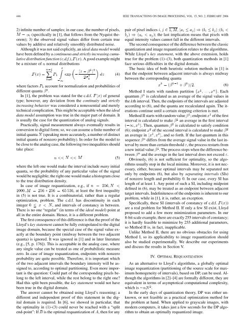
446 IEEE TRANSACTIONS ON IMAGE PROCESSING, VOL. 15, NO. 2, FEBRUARY 2006
2) infinite number of samples; in our case, the number of pixels,
(specifically in [1], that follows from the Nyquist theorem);
3) the observed signal values differ from certain true
values by additive and relatively smoothly distributed noise.
Although it was not said explicitly, an ideal data model would
have been defined by a continuous and strictly increasing cumulative
distribution function (c.d.f.), . A good example might
be a mixture of normal distributions
where factors account for normalization and probabilities of
different quanta .
In [1], the problem was stated for the c.d.f. of general
type; however, any deviation from the continuity and strictly
increasing behavior was considered a nonessential and merely
technical complication. This might be acceptable when the ideal
data model assumption was true in the major part of domain. It
is usually the case for the quantization of analog signals.
Practically, signal measurement always eventually results in
conversion to digital form; so, we can assume a finite number of
initial quanta (speaking more accurately, a number of distinct
initial quanta of nonzero probability). In order for the model to
be close to the analog case, the following two inequalities should
take place:
where the left one would make the interval include many initial
quanta, so the probability of any particular value of the signal
would be negligible; the right one would make a histogram close
to the true distribution density.
In case of image requantization, e.g., if
, at least the first inequality
in (5) is not true. It is a combinatorial, rather than a regular
optimization, problem. The c.d.f. has discontinuity in each
integer
, and intervals of constancy in between.
There is no one “regular” (in terms of the ideal model) point at
all in the entire domain. Hence, it is a different problem.
The first consequence of this difference is that the proof of the
Lloyd’s key statement cannot be fully extrapolated to the digital
image domain, because the special case of the signal value exactly
at the boundary point (midway between the two adjacent
quanta) is ignored. It was ignored in [1] and in later literature
(e.g., [5, p. 176]). This is acceptable in the analog case, where
any single value can be treated as one of probabilistic measure
zero. In case of image requantization, endpoints with nonzero
probability are quite possible. Therefore, it is important which
of the two adjacent intervals the boundary intensity will be assigned
to, according to optimal partitioning. Even more important
is the question: Could part of the corresponding pixels belong
to the left interval, while the rest belong to the right one?
Had this split been possible, the key statement would not have
been true in the digital domain.
The answer cannot be obtained using Lloyd’s reasoning; a
different and independent proof of this statement in the digital
domain is required. In [6], we showed in particular, that
the optimality in (1)–(3) could never be reached with a “split
end-point”:If is the optimal requantization of , then for any
(4)
(5)
pair of pixel indices
; the last implication means that pixels with
equal intensity values cannot fall in the different intervals.
The second consequence of the difference between the classic
quantization and image requantization relates to the algorithms.
While Lloyd’s key statement, with the above extension, holds
true for the problem (1)–(3), both quantization methods in [1]
face serious difficulties in the digital domain.
The basic idea of both heuristic solution methods in [1] is
that the endpoint between adjacent intervals is always midway
between the corresponding quanta
(6)
Method I starts with random partition
. Each
quantum is calculated as an average of the signal values in
the th interval. Then, the endpoints of the intervals are adjusted
according to (6), and the quanta are recalculated again. The iterations
continue until a certain stopping criterion is met.
Method II starts with random value ; endpoint of the first
interval is calculated to make an average in the first interval
. Then, quantum is calculated to satisfy condition
(6); endpoint of the second interval is calculated to make
an average in , and so forth. If the last quantum in this
sequence differs from the average signal value in the last interval
by more than certain threshold , the process restarts from
a new initial value . The process stops when the difference between
and the average in the last interval does not exceed .
Obviously, (6) is not sufficient for optimality, so the algorithms
usually stop in the local minima. Moreover, it is not necessary,
either, because optimal intervals may be separated not
only by endpoints (6), but also by separating intervals (SIs)
of nonzero length and probability 0. In our case, every SI has
length of at least 1. Any point of such a SI, including midpoint
defined in (6), may be treated as an endpoint between adjacent
target intervals. Indefiniteness of the endpoints is inherent to our
problem, while in [1], it is, rather, an exception.
Specifically, these SI (intervals of constancy of c.d.f. )
are a real problem for Method II. If only a few SI exist, Lloyd
proposed to add a few more minimization parameters. In our
8-bit scale example, there are exactly 255 intervals of constancy;
it is hardly feasible to minimize by 255 additional parameters,
so Method II is, in fact, inapplicable.
Unlike Method II, there are no obvious obstacles for using
Method I, so its applicability to image requantization should
also be studied experimentally. We describe our experiments
and discuss the results in Section V.
IV. OPTIMAL REQUANTIZATION
As an alternative to Lloyd’s algorithms, a globally optimal
image requantization (partitioning of the source scale for maximum
homogeneity of intervals), based on DP, can be used. Although
the algorithms in [2]–[4] are formally different, they are
equivalent in terms of asymptotical computational complexity,
which is .
In the early days of quantization theory, DP was either unknown,
or not feasible as a practical optimization method for
the problem at hand. When applied to grayscale images, with
modern computers, it takes just a few seconds for the DP algorithm
to obtain an optimally requantized image.