Optimal requantization of deep grayscale images and Lloyd-Max ...

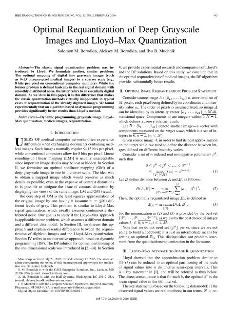
IEEE TRANSACTIONS ON IMAGE PROCESSING, VOL. 15, NO. 2, FEBRUARY 2006 445
Optimal Requantization of Deep Grayscale
Images and Lloyd–Max Quantization
Solomon M. Borodkin, Aleksey M. Borodkin, and Ilya B. Muchnik
Abstract—The classic signal quantization problem was introduced
by Lloyd. We formulate another, similar problem:
The optimal mapping of digital fine grayscale images (such
as 9–13 bits-per-pixel medical images) to a coarser scale (e.g.,
8 bits per pixel on conventional computer monitors). While the
former problem is defined basically in the real signal domain with
smoothly distributed noise, the latter refers to an essentially digital
domain. As we show in this paper, it is this difference that makes
the classic quantization methods virtually inapplicable in typical
cases of requantization of the already digitized images. We found
experimentally that an algorithm based on dynamic programming
provides significantly better results than Lloyd’s method.
Index Terms—Dynamic programming, grayscale image, Lloyd–
Max quantization, medical images, requantization.
I. INTRODUCTION
USERS OF medical computer networks often experience
difficulties when exchanging documents containing medical
images. Such images normally require 9–13 bits per pixel,
while conventional computers allow for 8 bits per pixel. Linear
rounding-up [linear mapping (LM)] is usually unacceptable
since important image details may be lost or hidden. In Section
II, we formulate an optimal nonlinear mapping (OM) of a
deep grayscale image to one in a coarser scale. The idea was
to obtain a mapped image which would preserve as much
details as possible, even at the expense of contrast distortions
(it is possible to mitigate the issue of contrast distortion by
displaying two views of the same image: LM and OM views).
The core step of OM is the least squares approximation of
the original image by one having (assume ) different
levels of gray. This problem is similar to Lloyd–Max
signal quantization, which usually assumes continuously distributed
noise. Our goal is to study if the Lloyd–Max approach
is applicable to our problem, which assumes a different domain
and a different data model. In Section III, we discuss this approach
and explain essential differences between the requantization
of digitized images and the Lloyd–Max quantization.
Section IV refers to an alternative approach, based on dynamic
programming (DP). The DP solution for optimal partitioning of
the one-dimensional scale was introduced in [2]–[4]. In Section
Manuscript received July 23, 2003; revised February 17, 2005. The associate
editor coordinating the review of this manuscript and approving it for publication
was Dr. Reiner Eschbach.
S. M. Borodkin is with the CACI Enterprise Solutions, Inc., Lanham, MD
20706 USA (e-mail: sborodkin@caci.com).
A. M. Borodkin is with the BAE Systems, Washington, DC 20212 USA
(e-mail: aleksey.borodkin@baesystems.com).
I. B. Muchnik is with the Computer Science Department, Rutgers University,
Piscataway, NJ 08854 USA (e-mail: muchnik@dimacs.rutgers.edu).
Digital Object Identifier 10.1109/TIP.2005.860611
V, we provide experimental research and comparison of Lloyd’s
and the DP solutions. Based on this study, we conclude that in
the optimal requantization of medical images, the DP algorithm
provides substantially better results.
II. OPTIMAL IMAGE REQUANTIZATION: PROBLEM STATEMENT
Consider source image
as an ordered set of
pixels, each pixel being defined by its coordinates and intensity
value . The order of pixels is assumed fixed, so image
can be identified by its intensity vector in -dimensional
space. Components are integers within ,
which defines a source intensity scale.
Let
denote another image—a vector with
components measured on the target scale, which is a set of integers
in .
Given source image , in order to find its best approximation
on the target scale, we need to define the distance between images
defined on different intensity scales.
Consider a set of ordered real nonnegative parameters ,
such that
Let define distance between and , as follows:
Then, the optimally requantized image
is defined as
So, the minimization in (2) and (3) is provided by the best set
, as well as by the best choice of integer
values .
Note that we do not need set per se, since we are not
going to build a codebook; it is just an intermediate means for
getting an optimal . This distinguishes our problem statement
from the quantization/requantization in the literature.
III. LLOYD–MAX APPROACH TO IMAGE REQUANTIZATION
Lloyd showed that the approximation problem similar to
(1)–(3) can be reduced to an optimal partitioning of the scale
of signal values into disjunctive semi-open intervals. This
is a key statement in [1], and will be referred to thus below.
The direct consequence is that for each , the optimal is the
mean signal value in the th interval.
The key statement is based on the following data model: 1) the
observed signal values are real numbers; in our terms, ;
(1)
(2)
(3)
1057-7149/$20.00 © 2006 IEEE

446 IEEE TRANSACTIONS ON IMAGE PROCESSING, VOL. 15, NO. 2, FEBRUARY 2006
2) infinite number of samples; in our case, the number of pixels,
(specifically in [1], that follows from the Nyquist theorem);
3) the observed signal values differ from certain true
values by additive and relatively smoothly distributed noise.
Although it was not said explicitly, an ideal data model would
have been defined by a continuous and strictly increasing cumulative
distribution function (c.d.f.), . A good example might
be a mixture of normal distributions
where factors account for normalization and probabilities of
different quanta .
In [1], the problem was stated for the c.d.f. of general
type; however, any deviation from the continuity and strictly
increasing behavior was considered a nonessential and merely
technical complication. This might be acceptable when the ideal
data model assumption was true in the major part of domain. It
is usually the case for the quantization of analog signals.
Practically, signal measurement always eventually results in
conversion to digital form; so, we can assume a finite number of
initial quanta (speaking more accurately, a number of distinct
initial quanta of nonzero probability). In order for the model to
be close to the analog case, the following two inequalities should
take place:
where the left one would make the interval include many initial
quanta, so the probability of any particular value of the signal
would be negligible; the right one would make a histogram close
to the true distribution density.
In case of image requantization, e.g., if
, at least the first inequality
in (5) is not true. It is a combinatorial, rather than a regular
optimization, problem. The c.d.f. has discontinuity in each
integer
, and intervals of constancy in between.
There is no one “regular” (in terms of the ideal model) point at
all in the entire domain. Hence, it is a different problem.
The first consequence of this difference is that the proof of the
Lloyd’s key statement cannot be fully extrapolated to the digital
image domain, because the special case of the signal value exactly
at the boundary point (midway between the two adjacent
quanta) is ignored. It was ignored in [1] and in later literature
(e.g., [5, p. 176]). This is acceptable in the analog case, where
any single value can be treated as one of probabilistic measure
zero. In case of image requantization, endpoints with nonzero
probability are quite possible. Therefore, it is important which
of the two adjacent intervals the boundary intensity will be assigned
to, according to optimal partitioning. Even more important
is the question: Could part of the corresponding pixels belong
to the left interval, while the rest belong to the right one?
Had this split been possible, the key statement would not have
been true in the digital domain.
The answer cannot be obtained using Lloyd’s reasoning; a
different and independent proof of this statement in the digital
domain is required. In [6], we showed in particular, that
the optimality in (1)–(3) could never be reached with a “split
end-point”:If is the optimal requantization of , then for any
(4)
(5)
pair of pixel indices
; the last implication means that pixels with
equal intensity values cannot fall in the different intervals.
The second consequence of the difference between the classic
quantization and image requantization relates to the algorithms.
While Lloyd’s key statement, with the above extension, holds
true for the problem (1)–(3), both quantization methods in [1]
face serious difficulties in the digital domain.
The basic idea of both heuristic solution methods in [1] is
that the endpoint between adjacent intervals is always midway
between the corresponding quanta
(6)
Method I starts with random partition
. Each
quantum is calculated as an average of the signal values in
the th interval. Then, the endpoints of the intervals are adjusted
according to (6), and the quanta are recalculated again. The iterations
continue until a certain stopping criterion is met.
Method II starts with random value ; endpoint of the first
interval is calculated to make an average in the first interval
. Then, quantum is calculated to satisfy condition
(6); endpoint of the second interval is calculated to make
an average in , and so forth. If the last quantum in this
sequence differs from the average signal value in the last interval
by more than certain threshold , the process restarts from
a new initial value . The process stops when the difference between
and the average in the last interval does not exceed .
Obviously, (6) is not sufficient for optimality, so the algorithms
usually stop in the local minima. Moreover, it is not necessary,
either, because optimal intervals may be separated not
only by endpoints (6), but also by separating intervals (SIs)
of nonzero length and probability 0. In our case, every SI has
length of at least 1. Any point of such a SI, including midpoint
defined in (6), may be treated as an endpoint between adjacent
target intervals. Indefiniteness of the endpoints is inherent to our
problem, while in [1], it is, rather, an exception.
Specifically, these SI (intervals of constancy of c.d.f. )
are a real problem for Method II. If only a few SI exist, Lloyd
proposed to add a few more minimization parameters. In our
8-bit scale example, there are exactly 255 intervals of constancy;
it is hardly feasible to minimize by 255 additional parameters,
so Method II is, in fact, inapplicable.
Unlike Method II, there are no obvious obstacles for using
Method I, so its applicability to image requantization should
also be studied experimentally. We describe our experiments
and discuss the results in Section V.
IV. OPTIMAL REQUANTIZATION
As an alternative to Lloyd’s algorithms, a globally optimal
image requantization (partitioning of the source scale for maximum
homogeneity of intervals), based on DP, can be used. Although
the algorithms in [2]–[4] are formally different, they are
equivalent in terms of asymptotical computational complexity,
which is .
In the early days of quantization theory, DP was either unknown,
or not feasible as a practical optimization method for
the problem at hand. When applied to grayscale images, with
modern computers, it takes just a few seconds for the DP algorithm
to obtain an optimally requantized image.

BORODKIN et al.: OPTIMAL REQUANTIZATION OF DEEP GRAYSCALE IMAGES 447
Fig. 1.
Image MR-ANGIO, [7]. (a) Linearly mapped image; D = 94 376:01. (b) Best image obtained by Method I, with randomly generated initial conditions;
seed = 10; D = 23 364:43. (c) Worst image obtained by Method I; trial 99, D = 583 217:56. (d) Optimal requantization; D = 6757:28.
TABLE I
SUMMARY OF EXPERIMENTAL STUDY OF LLOYD’S METHOD I
In our experimental study, we used the algorithm provided in
[6], which is close to [3].
V. EXPERIMENTAL RESULTS
We studied Lloyd’s Method I experimentally. We used an
11-bit, 256 256 medical image [7], where only 632 intensity
values out of 2048 had nonzero probability, in the range
of 0–1365. The result of the linear mapping to 8-bit grayscale is
presented in Fig. 1(a).
One hundred eleven trials were made in total using various
initial conditions, in order to obtain 100 successful trials; 11
trials were prematurely terminated because an empty interval
occurred during the iterations. An empty interval is a known
complication of Method I, which, however, was viewed as a
merely technical and virtually unlikely one [1]. We did not use
modifications of the algorithm to handle these situations; we
simply terminated the trial and excluded it from the results in
order to study a "pure" Method I.
The experimental results are summarized in Table I.
In trials 1–98, initial intervals were built at random, with uniform
distribution and different seed values of the generator of
pseudo-random numbers. Care was taken to make each initial
interval nonempty (improper random values were skipped).
In trial 99, initial intervals were chosen as follows: first 255
intervals contained single values 0,1,2, ,254, respectively; the
last interval contained values 255 through the maximum, 1365.
In trial 100, for initial partitioning, we used an optimal partitioning,
obtained by the DP algorithm.
The following observations have been made.
1) All of the obtained 100 solutions were different.
2) Only trial 100 resulted in the optimal solution. (Note:
Had it happened a boundary intensity value assigned to

448 IEEE TRANSACTIONS ON IMAGE PROCESSING, VOL. 15, NO. 2, FEBRUARY 2006
incorrect interval, Method I would have pulled away from
the optimal starting partition and eventually would have
stopped at a nonoptimal one; that did not happen).
3) While the optimal value of was 6757.28, the
range of values obtained in trials 1–98 was 23 364.43
through 57 012.44. In trial 99, it was 583 217.56. For the
linear mapping,
. In all trials, the greater
initial (corresponding to initial partition), the greater
the final value of criterion .
4) All of the images obtained in trials 1–99 are visually worse
thantheoptimalimageFig.1(d).By“worse,”wemeanthat
lessimagedetailarevisuallydistinguishableinthepicture.
As a rule, the greater value, the worse the picture
visually.
Fig. 1(b) presents the best image, obtained in trials 1–99;
Fig. 1(c) presents the worst of the images obtained in trials 1–99
(no details can be distinguished in the white area.)
One can see that the OM image Fig. 1(d) contains image detail
that is invisible even in the best image Fig. 1(b) obtained by
Lloyd’s Method I in trials 1–99.
The reason for this behavior is that with
, condition (5) is not met. There is no sufficient leeway for
Method I to improve initial partitioning. The algorithm usually
stops after just a few iterations (6–8 in most of our experiments).
That does not happen in the real [or digital, provided (5)] domain,
where fine endpoint positioning may allow for a long iteration
process, thus providing a potentially better solution.
The following example illustrates this in more detail. Assume
that before the current iteration, the endpoint between the adjacent
intervals was 5.1; after recalculation of , followed
by recalculation of endpoints according to (6), we obtain a new
endpoint 5.9, while all the other endpoints did not change. After
this iteration, the algorithm will stop, because the interval between
5.0 and 6.0 is its “zone of insensitivity.” Repositioning of
the endpoint from 5.1 to 5.9 will not cause further changes and
a continuation of iterations.
As a result, the obtained images are highly dependent on the
initial conditions of Method I.
VI. CONCLUSION
We introduced a formal statement of the image requantization
problem, which is close to the Lloyd–Max signal quantization.
However, there exists a substantial difference between the two.
Lloyd–Max quantization is based on the idea that endpoints
of optimal intervals are located midway between the corresponding
quanta (6). Generally, it is neither necessary nor
sufficient for optimality. It works in the real domain, in the case
of distribution without singularities and intervals of constancy
of c.d.f., or in the digital domain (5).
When we switch to image requantization, with nothing but
discontinuity points and intervals of constancy being a c.d.f. domain,
and with (5) being false, the key statement (the equivalence
of the signal approximation problem and the optimal partitioning
of signal scale) holds true, but it does not follow from
the simplified reasoning in [1]. An independent proof in [6] provides
an accurate treatment of all cases, including those having
probability 0 in the real domain.
As for the two classic heuristic solution methods for suboptimal
partitioning [1], the first one shows rather poor behavior
in the case of image requantization; the second one is, in fact,
inapplicable.
A globally optimal solution, based on DP, seems to be a real
alternative for image requantization.
There also exist numerous suboptimal heuristic algorithms,
which may work on images significantly better than Lloyd’s
quantization; that was beyond the scope of this paper.
REFERENCES
[1] S. P. Lloyd, “Least squares quantization in PCM,” IEEE Trans. Inf.
Theory, vol. IT-28, no. 2, pp. 129–137, Mar. 1982.
[2] W. D. Fisher, “On grouping for maximum homogeneity,” J. Amer. Stat.
Assoc., vol. 53, pp. 789–798, 1958.
[3] S. M. Borodkin, “Optimal grouping of interrelated ordered objects,”
in Automation and Remote Control. New York: Plenum, 1980, pp.
269–276.
[4] S. Kundu, “A solution to histogram-equalization and other related problems
by shortest path methods,” Pattern Recognit., vol. 31, no. 3, pp.
231–234, Mar. 1998.
[5] A. Gersho and R. M. Gray, Vector Quantization And Signal Processing.
Norwell, MA: Kluwer, 1992.
[6] S. Borodkin, A. Borodkin, and I. Muchnik. (2004, Nov.) Optimal
Mapping of Deep Gray Scale Images to a Coarser Scale. Rutgers Univ.,
Piscataway, NJ. [Online]. Available: ftp://dimacs.rutgers.edu/pub/dimacs/TechnicalReports/2004/2004-53.pdf
[7] Source Image [Online]. Available: ftp://ftp.erl.wustl.edu/pub/dicom/images/version3/other/philips/mr-angio.dcm.Z
Solomon M. Borodkin received the M.S. and Ph.D.
degrees in technical cybernetics from the Moscow Institute
of Physics and Technology, Moscow, Russia,
in 1970 and 1975, respectively.
From 1970 to 1993, he worked on data analysis
methods, computational algorithms, software development
in the field of control systems, social studies,
and neuroscience (signal and image processing).
Since 1994, he has worked on mathematical
problems and software development for document
imaging and workflow systems. His research interests
include models and applications of discrete mathematics, computational procedures
for dynamic programming, and image compression and presentation.
Aleksey M. Borodkin received the M.S. and Ph.D.
degrees in technical cybernetics from the Moscow
Institute of Physics and Technology, Moscow,
Russia, 1973 and 1980, respectively. From 1973 to
1993, he worked on optimization methods in data
analysis and software development for computerized
control systems.
Since 1993, he has been involved in research and
software development for image analysis and large
statistical surveys. His research interests include
image processing and combinatorial optimization.
Ilya B. Muchnik received the M.S. degree in
radio physics from the State University of Nizhny
Novgorod, Russia in 1959, and the Ph.D. degree in
technical cybernetics from the Institute of Control
Sciences, Moscow, Russia, in 1971.
From 1960 to 1990, he was with the Moscow
Institute of Control Sciences, Moscow, Russia. In
the early days of the pattern recognition and machine
learning, he developed the algorithms for machine
understanding of structured images. In 1972, he proposed
a method for the shape-content contour pixel
localization. He developed new combinatorial clustering models and worked
on their applications for multidimensional data analysis in social sciences,
economy, biology, and medicine. Since 1993, he has been a Research Professor
with the Computer Science Department, Rutgers University, Piscataway, NJ,
where he teaches pattern recognition, clustering, and data visualization for bioinformatics.
His research interests include machine understanding of structured
data and data imaging and large-scale combinatorial optimization methods.