Impurity problems for steady-state nonequilibrium dynamical mean ...
Impurity problems for steady-state nonequilibrium dynamical mean ...
Impurity problems for steady-state nonequilibrium dynamical mean ...

You also want an ePaper? Increase the reach of your titles
YUMPU automatically turns print PDFs into web optimized ePapers that Google loves.
ARTICLE IN PRESS<br />
Physica E 42 (2010) 520–524<br />
Contents lists available at ScienceDirect<br />
Physica E<br />
journal homepage: www.elsevier.com/locate/physe<br />
<strong>Impurity</strong> <strong>problems</strong> <strong>for</strong> <strong>steady</strong>-<strong>state</strong> <strong>nonequilibrium</strong> <strong>dynamical</strong><br />
<strong>mean</strong>-field theory<br />
J.K. Freericks<br />
Department of Physics, Georgetown University, Washington, DC 20057, USA<br />
article info<br />
Available online 24 June 2009<br />
Keywords:<br />
Nonequilibrium many-body physics<br />
Dynamical <strong>mean</strong>-field theory<br />
Steady <strong>state</strong><br />
Functional methods<br />
abstract<br />
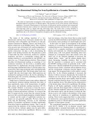
The mapping of <strong>steady</strong>-<strong>state</strong> <strong>nonequilibrium</strong> <strong>dynamical</strong> <strong>mean</strong>-field theory from the lattice to the<br />
impurity is described in detail. Our focus is on the case with current flow under a constant dc electric<br />
field of arbitrary magnitude. In addition to <strong>for</strong>mulating the problem via path integrals and functional<br />
derivatives, we also describe the distribution-function dependence of the retarded and advanced<br />
Green’s functions. Our <strong>for</strong>mal developments are exact <strong>for</strong> the Falicov–Kimball model. We also show how<br />
these <strong>for</strong>mal developments are modified <strong>for</strong> more complicated models (like the Hubbard model).<br />
& 2009 Elsevier B.V. All rights reserved.<br />
1. Introduction<br />
Dynamical <strong>mean</strong>-field theory (DMFT) began in 1989, when<br />
Metzner and Vollhardt suggested the large-dimensional limit<br />
(with an appropriate rescaling of the hopping integral) as a<br />
simplifying limit <strong>for</strong> the many-body problem that nevertheless<br />
still included the important competition between minimizing the<br />
kinetic and potential energies of the system [1]. These ideas were<br />
implemented into a complete DMFT by Brandt and Mielsch with<br />
the exact solution of the Falicov–Kimball model at half filling [2].<br />
Since that time, nearly all equilibrium many-body models have<br />
been solved in the large-dimensional limit with DMFT. Recently,<br />
progress has been made on <strong>nonequilibrium</strong> extensions of DMFT<br />
[3–7] <strong>for</strong> the Falicov–Kimball model and <strong>for</strong> the Hubbard model<br />
[8]. In situations where the perturbing fields (or the timedependent<br />
part of the Hamiltonian) maintains the translational<br />
invariance of the lattice, the self-energy remains uni<strong>for</strong>m and<br />
local, as follows from the Langreth rules [9] and the perturbative<br />
expansion in the hopping by Metzner [10].<br />
In this work, we examine the <strong>steady</strong>-<strong>state</strong> limit of <strong>nonequilibrium</strong><br />
DMFT. We start the system in equilibrium at an inverse<br />
temperature b and wait a long time after the field or timedependence<br />
has been turned on, so that the system has<br />
reorganized itself to the long-time response of the driving fields<br />
(or time dependence) [11,12]. We are inherently assuming that the<br />
long-time limit of the Hamiltonian is different from the original<br />
equilibrium Hamiltonian. It need not have any explicit time<br />
dependence in this limit though. We will show that the Keldysh<br />
<strong>for</strong>mulation of the many-body theory [ignoring the third<br />
(imaginary) branch of the contour described by Wagner [13]]<br />
E-mail address: freericks@physics.georgetown.edu<br />
produces the exact <strong>steady</strong>-<strong>state</strong> solution <strong>for</strong> the Falicov–Kimball<br />
model; we will also discuss modifications <strong>for</strong> the Hubbard model<br />
(and more complicated models). Our approach works with<br />
functional integrals and derivatives. Most of the techniques are<br />
completely straight<strong>for</strong>ward, but these details have not appeared<br />
in the literature yet, and provide useful insights into the solution<br />
of <strong>nonequilibrium</strong> <strong>problems</strong> via DMFT.<br />
2. Formalism <strong>for</strong> the Falicov–Kimball model<br />
We will focus our ef<strong>for</strong>ts first on the Falicov–Kimball<br />
model, whose Hamiltonian [15] is the following (in a uni<strong>for</strong>m<br />
electric field described by a uni<strong>for</strong>m vector potential E ¼<br />
@AðtÞ=c@t):<br />
H FK ¼ X k<br />
fe½k eAðtÞ=‘ cŠ mgc y k c k þ U X i<br />
c y i c iw i ;<br />
where we employed Peierls’ substitution [14]. Here, c k<br />
and c y k<br />
destroy and create a<br />
p<br />
spinless itinerant fermion with momentum k,<br />
eðkÞ ¼ lim d-1 ðt = ffiffiffi P<br />
d Þ d<br />
i¼1 cosk i is the bandstructure on an<br />
infinite-dimensional hypercubic lattice, m is the itinerant-electron<br />
chemical potential, U is the conduction-electron–local-electron<br />
interaction, w i is the number operator <strong>for</strong> the spinless localized<br />
electrons at site i, and we use the real-space basis <strong>for</strong> the itinerant<br />
electron operators in the second term of H. In the following we<br />
set ‘ ¼ c ¼ t ¼ 1.<br />
We are interested in the <strong>steady</strong>-<strong>state</strong> limit of the response,<br />
which can be determined in the limit where the vector potential is<br />
turned on in the infinite past (but after the system has fully<br />
equilibrated into an equilibrium distribution with inverse temperature<br />
b); in other words, we choose AðtÞ ¼lim t0 - 1y<br />
ðt t 0 Þðt t 0 ÞE. In <strong>nonequilibrium</strong> physics there are two different<br />
ð1Þ<br />
1386-9477/$ - see front matter & 2009 Elsevier B.V. All rights reserved.<br />
doi:10.1016/j.physe.2009.06.036
ARTICLE IN PRESS<br />
J.K. Freericks / Physica E 42 (2010) 520–524 521<br />
Green’s functions that are required to describe the system. One is<br />
the retarded Green’s function and the other is the Keldysh Green’s<br />
function. The <strong>for</strong>mer describes how the quantum density of <strong>state</strong>s<br />
(DOS) varies with energy, while the latter describes how the<br />
electrons are distributed amongst those <strong>state</strong>s. Naively, one<br />
would assume that the quantum <strong>state</strong>s would be independent<br />
of the initial temperature, although they will depend on the<br />
electric field strength, the fillings of the particles, and the<br />
interaction energy. But it is well known in equilibrium manybody<br />
physics that interacting systems often display some<br />
temperature dependence to the DOS. Noninteracting <strong>problems</strong>,<br />
and the Falicov–Kimball model are exceptions, however, where<br />
the DOS is independent of how the electrons are distributed<br />
amongst the <strong>state</strong>s. It is the goal of this work to elaborate on this<br />
situation in <strong>nonequilibrium</strong> cases.<br />
Our starting point is to define the contour-ordered Green’s<br />
function on the two-branch Keldysh contour, which runs from<br />
t ¼ 1 to 1 and back. We define it only <strong>for</strong> the case of<br />
an impurity in a time-dependent <strong>dynamical</strong> <strong>mean</strong> field<br />
denoted l C :<br />
G C ðt; t 0 Þ¼ iTr cf fT C r imp Sðl C ÞcðtÞc y ðt 0 Þg=Z; ð2Þ<br />
with r imp the <strong>steady</strong>-<strong>state</strong> density matrix <strong>for</strong> the impurity, the<br />
operators denote time evolution in the Heisenberg picture with<br />
respect to the impurity Hamiltonian H imp ¼ mc y c þ Uw i c y c,<br />
the S-matrix (evolution operator) satisfies<br />
Z Z<br />
<br />
Sðl C Þ¼T C exp i dt dt 0 c y ðtÞl C ðt; t 0 Þcðt 0 Þ ; ð3Þ<br />
C<br />
C<br />
Z ¼ Tr cf r imp<br />
T C Sðl C Þ is the partition function, the time ordering<br />
is with respect to the ordering along the contour, and the trace is<br />
over the four <strong>state</strong>s of the spinless conduction and localized<br />
electrons. The long-time-limit density matrix is aprioriunknown<br />
(while the lambda field is determined self-consistently with the<br />
DMFT algorithm). In practice, one needs to evolve the full manybody<br />
system from the time the field is turned on until the longtime<br />
limit is reached (and use the so-called restart theorem [16]<br />
to determine it). We will see, however, that the density matrix<br />
does not enter into the calculation of retarded or advanced<br />
quantities <strong>for</strong> the Falicov–Kimball model, so we defer further<br />
discussion at the moment. We will work with Wigner coordinates<br />
[17] of average T ¼ðt þ t 0 Þ=2 and relative t rel ¼ t t 0 time<br />
below.<br />
We begin our discussion by considering a problem that has no<br />
localized particles, so we do not take the trace over the f -<br />
electrons, but instead, simply set w i ¼ 0. The full solution,<br />
including the trace over f-particles can be easily constructed from<br />
this solution, as we show below. It is convenient to break up the<br />
two-branch contour into a þ branch, where the time increases<br />
from 1 to þ1 and a minus branch, where time decreases<br />
from þ1 to 1. Then the evolution operator in Eq. (3) can be<br />
rewritten as<br />
<br />
Sðl C Þ¼T C exp<br />
Z 1 Z 1<br />
i dt dt 0 fcþðtÞl y T ðt; t 0 Þc þ ðt 0 Þ<br />
1 1<br />
c y ðtÞl 4 ðt; t 0 Þc þ ðt 0 Þ<br />
i<br />
; ð4Þ<br />
c y þðtÞl o ðt; t 0 Þc ðt 0 Þ<br />
þc y ðtÞl T ðt; t 0 Þc ðt 0 Þg<br />
the four different Green’s functions are defined as follows (we<br />
suppress the trace over the f -electrons, which is needed <strong>for</strong> the<br />
Falicov–Kimball model, but is neglected <strong>for</strong> the moment):<br />
G T ðt; t 0 Þ¼ iTr c fT t r imp<br />
Sðl C Þc þ ðtÞcþðt y 0 Þg=Z; ð5Þ<br />
G T ðt; t 0 Þ¼ iTr c fT t<br />
r imp Sðl C Þc ðtÞc y ðt 0 Þg=Z; ð6Þ<br />
G o ðt; t 0 Þ¼iTr c fr imp Sðl C Þc y þðt 0 Þc ðtÞg=Z;<br />
G 4 ðt; t 0 Þ¼ iTr c fr imp Sðl C Þc þ ðtÞc y ðt 0 Þg=Z; ð8Þ<br />
where the t and t subscripts denote time-ordering or anti-timeordering,<br />
respectively. The retarded and advanced Green’s functions<br />
are defined to be G r ¼ G T G o and G a ¼ G T þ G o , which<br />
can be written as<br />
G r ðt; t 0 Þ¼ iyðt t 0 ÞTr c ½r imp<br />
Sðl C ÞfcðtÞ; c y ðt 0 Þg þ Š; ð9Þ<br />
G a ðt; t 0 Þ¼iyðt 0 tÞTr c ½r imp Sðl C ÞfcðtÞ; c y ðt 0 Þg þ Š; ð10Þ<br />
in terms of the operators. Similarly, the Keldysh and anti-Keldysh<br />
Green’s functions are defined to be G K ¼ G 4 þ G o and G K ¼ G T<br />
G T þ G 4 þ G o ,or<br />
G K ðt; t 0 Þ¼ iTr c fr imp<br />
Sðl C Þ½cðtÞ; c y ðt 0 ÞŠ g; ð11Þ<br />
G K ðt; t 0 Þ¼ iTr c fr imp Sðl C Þf½cðtÞ; c y ðt 0 ÞŠ ½cðtÞ; c y ðt 0 ÞŠ gg: ð12Þ<br />
Note that the anti-Keldysh Green’s function vanishes, but we need<br />
its functional <strong>for</strong>m in order to take functional derivatives <strong>for</strong><br />
different Green’s functions below. Using the definition of the<br />
evolution operator, we immediately find that the Green’s functions<br />
can be found as functional derivatives of the partition<br />
function. The explicit relations are<br />
G T ðt; t 0 dlnZ<br />
Þ¼<br />
dl T ðt 0 ; tÞ ; GT ðt; t 0 dlnZ<br />
Þ¼<br />
; ð13Þ<br />
dl T ðt 0 ; tÞ<br />
G o ðt; t 0 Þ¼<br />
dlnZ<br />
dl 4 ðt 0 ; tÞ ; G4 ðt; t 0 Þ¼ dlnZ<br />
dl o ðt 0 ; tÞ ;<br />
ð7Þ<br />
ð14Þ<br />
<strong>for</strong> the time-ordered, anti-time-ordered, lesser, and greater<br />
Green’s functions, respectively. We will discuss the alternative<br />
retarded, advanced, Keldysh and anti-Keldysh basis below. Now<br />
that we have all of these definitions, we can actually solve<br />
explicitly <strong>for</strong> these Green’s functions using the equations of<br />
motion (EOMs). We take the definition of the Green’s function,<br />
and differentiate with respect to time; where appropriate,<br />
one needs to take into account the time ordering, which<br />
brings down terms proportional to the l fields. This procedure<br />
is straight<strong>for</strong>ward to complete, and the end result is the<br />
following:<br />
Z 1<br />
i@ t G T ðt; t 0 Þ¼dðt t 0 Þ mG T ðt; t 0 Þþ dtl T ðt; tÞG T ðt; t 0 Þ<br />
Z<br />
1<br />
1<br />
dtl o ðt; tÞG 4 ðt; t 0 Þ;<br />
ð15Þ<br />
1<br />
Z 1<br />
i@ t G T ðt; t 0 Þ¼dðt t 0 ÞþmG T ðt; t 0 Þ dtl 4 ðt; tÞG o ðt; t 0 Þ<br />
1<br />
where the fermionic operators with the þ or subscript live on<br />
the corresponding time branch; the minus sign enters from the<br />
change of direction in how the time evolves on the two different<br />
branches. When both time arguments lie on the þ branch or the<br />
branch, we have time-ordered (T) or anti-time-ordered ðT Þ<br />
objects, respectively. When one is on the þ and one on the ,<br />
we have the lesser (o) or greater ð4Þ functions. To be concrete,<br />
i@ t G o ðt; t 0 Þ¼<br />
Z 1<br />
þ dtl T ðt; tÞG T ðt; t 0 Þ;<br />
1<br />
Z 1<br />
mG o ðt; t 0 Þþ dtl T ðt; tÞG o ðt; t 0 Þ<br />
1<br />
Z 1<br />
dtl o ðt; tÞG T ðt; t 0 Þ;<br />
1<br />
ð16Þ<br />
ð17Þ
ARTICLE IN PRESS<br />
522<br />
J.K. Freericks / Physica E 42 (2010) 520–524<br />
i@ t G 4 ðt; t 0 Þ¼mG 4 ðt; t 0 Þ<br />
Z 1<br />
þ dtl T ðt; tÞG 4 ðt; t 0 Þ;<br />
1<br />
Z 1<br />
dtl 4 ðt; tÞG T ðt; t 0 Þ<br />
1<br />
ð18Þ<br />
with similar equations <strong>for</strong> derivatives with respect to t 0 which<br />
we do not write down explicitly.<br />
On the lattice, one can exactly solve <strong>for</strong> the analogous contourordered<br />
Green’s functions in the case where U ¼ 0 [18]. One can<br />
see from the exact solution, that the noninteracting retarded<br />
Green’s function becomes average time independent <strong>for</strong> long<br />
times after the field has been turned on. We make the ansatz that<br />
the retarded self-energy is also independent of average time in the<br />
long-time limit (which is consistent with gauge-invariance<br />
arguments [19,20,7], but is an independent ansatz). Then, it is<br />
straight<strong>for</strong>ward to show that the interacting retarded Green’s<br />
function is independent of average time. In general, we can only<br />
show that the average time dependence of the contour-ordered<br />
Green’s function is periodic in average time with a period given by<br />
the Bloch period 2p=E [8]. This allows us to make a continuous<br />
Fourier trans<strong>for</strong>m with respect to the relative time (frequency<br />
dependence o) and a discrete Fourier trans<strong>for</strong>m with respect to<br />
the average time (Fourier components no B ¼ nE) <strong>for</strong> all of the<br />
different components of the contour-ordered objects (timeordered,<br />
anti-time-ordered, lesser, greater, and Keldysh); the<br />
retarded and advanced components depend only on the continuous<br />
frequency o.<br />
In order to find the Green’s functions, we need to employ the<br />
simplification from the retarded and advanced Green’s functions,<br />
which depend only on the relative time, or frequency o. Hence,<br />
we need the EOM <strong>for</strong> the retarded and advanced functions, which<br />
can easily be shown to satisfy<br />
Z 1<br />
ði@ t þ mÞG r ðtÞ ¼dðtÞþ dtl r ðt tÞG r ðtÞ; ð19Þ<br />
1<br />
with<br />
<br />
D o þ n 2 o B; o<br />
n 2 o h<br />
B ¼ o þ n 2 o <br />
B þ m l r o þ n 2 o i<br />
B<br />
h<br />
o n 2 o <br />
B þ m l a o n 2 o i<br />
B : ð25Þ<br />
Similarly, we have<br />
G 4 l 4 ðno<br />
ðno B ; oÞ<br />
B ; oÞ ¼ <br />
D o þ n 2 o B; o<br />
n 2 o ; ð26Þ<br />
B<br />
and G T ðno B ; oÞ ¼G o ðno B ; oÞþd n0 G r ðoÞ and G T ðno B ; oÞ ¼<br />
G o ðno B ; oÞ d n0 G a ðoÞ; the Kronecker delta functions enter<br />
because the retarded and advanced Green’s functions are<br />
independent of average time. One can directly show that<br />
l T ðno b ; oÞ ¼l T ðno b ; oÞ ¼l o ðno b ; oÞ ¼l 4 ðno b ; oÞ;<br />
ð27Þ<br />
<strong>for</strong> na0. Now replacing the retarded and advanced quantities in<br />
the denominator by the time-ordered, anti-time-ordered, lesser<br />
and greater quantities, gives<br />
h<br />
D ¼ o þ n 2 o <br />
B þ m l T 0; o þ n 2 o i<br />
B<br />
h<br />
o n 2 o <br />
B þ m l T 0; o n 2 o i<br />
B<br />
<br />
þl o 0; o þ n 2 o h<br />
<br />
B no B þ l 4 0; o n 2 o i<br />
B ; ð28Þ<br />
which involves just the zeroth component of the Fourier series<br />
terms <strong>for</strong> the <strong>dynamical</strong> <strong>mean</strong> fields.<br />
Finally, we can now solve the functional differential equations,<br />
which take the <strong>for</strong>m Gðno b :oÞ ¼7dlnZ=dlð no B ; oÞ, and determine<br />
the partition function as<br />
Z<br />
lnZ ¼ doln½ðo þ m l T ð0; oÞÞðo þ m þ l T ð0; oÞÞ<br />
þl o ð0; oÞl 4 ð0; oÞŠ þ C<br />
Z 1<br />
ði@ t þ mÞG a ðtÞ ¼dðtÞþ dtl a ðt tÞG a ðtÞ; ð20Þ<br />
1<br />
and are solved by<br />
G r 1<br />
ðoÞ ¼<br />
o þ m l r ðoÞ ; 1<br />
Ga ðoÞ ¼<br />
o þ m l a ðoÞ ; ð21Þ<br />
where we have solved the problem in frequency space after a<br />
Fourier trans<strong>for</strong>mation. Next, we can show, by using the identities<br />
that relate the different quantities (T, T , o, 4, r, and a) to each<br />
other, that the EOM <strong>for</strong> G o becomes<br />
Z 1<br />
ði@ t þ mÞG o ðt; t 0 Þ¼ dtl r ðt tÞG o ðt; t 0 Þ<br />
1<br />
Z 1<br />
þ dtl o ðt; tÞG a ðt t 0 Þ; ð22Þ<br />
1<br />
since l T ¼ l r þ l o and G T ¼ G o G a . Substituting in the appropriate<br />
Fourier expansions then yields<br />
<br />
o þ n 2 o <br />
<br />
B G o ðno B ; oÞ ¼l r o þ n 2 o <br />
B G o ðno B ; oÞ<br />
<br />
þl o ðno B ; oÞG a o n 2 o <br />
B : ð23Þ<br />
This can be directly solved to yield<br />
G o l o ðno<br />
ðno B ; oÞ<br />
B ; oÞ ¼ <br />
D o þ n 2 o B; o<br />
n 2 o ; ð24Þ<br />
B<br />
þ X l o ðno B ; oÞl 4 ð no B ; oÞ l T ðno B ; oÞl T ð no B ; oÞ<br />
<br />
na0<br />
D o þ n 2 o B; o<br />
n 2 o ;<br />
B<br />
ð29Þ<br />
where we fix an undetermined constant C by equating with the<br />
noninteracting result. It is a straight<strong>for</strong>ward exercise to show that<br />
the functional derivatives of this partition function yield the<br />
Green’s functions.<br />
Our next step is to repeat these results <strong>for</strong> the alternative r, a,<br />
K, K basis. To start, the evolution operator becomes<br />
Z<br />
i 1 Z 1<br />
Sðl C Þ¼T t exp dt dt 0<br />
2 1 1<br />
ð½c y þðtÞ<br />
c y ðtÞŠl r ðt; t 0 Þ½c þ ðt 0 Þþc ðt 0 ÞŠ<br />
þ½c y þðtÞþc y ðtÞŠl a ðt; t 0 Þ½c þ ðt 0 Þ<br />
c ðt 0 ÞŠ<br />
þ½cþðtÞ y c y ðtÞŠl K ðt; t 0 Þ½c þ ðt 0 Þ c ðt 0 ÞŠ<br />
o<br />
þ½cþðtÞþc y y ðtÞŠl K ðt; t 0 Þ½c þ ðt 0 Þþc ðt 0 ÞŠÞ ; ð30Þ<br />
where we have added a new field l K which will be set equal to<br />
zero <strong>for</strong> all physical matrix elements that we evaluate. Using the<br />
definitions <strong>for</strong> the retarded, advanced, Keldysh and anti-Keldysh<br />
Green’s functions shows that we can determine them via<br />
functional derivatives<br />
G r ðt; t 0 Þ¼<br />
dlnZ<br />
dl r ðt 0 ; tÞ ;<br />
Ga ðt; t 0 Þ¼<br />
dlnZ<br />
dl a ðt 0 ; tÞ ;<br />
ð31Þ
ARTICLE IN PRESS<br />
J.K. Freericks / Physica E 42 (2010) 520–524 523<br />
G K ðt; t 0 Þ¼<br />
dlnZ<br />
; G K ðt; t 0 Þ¼<br />
dl K ðt 0 ; tÞ<br />
dlnZ<br />
dl K ðt 0 ; tÞ ;<br />
ð32Þ<br />
where all derivatives must be evaluated with l K ¼ 0 after taking<br />
the derivatives. Since we have already determined the retarded<br />
and advanced Green’s functions when we solved <strong>for</strong> the Green’s<br />
functions in the other basis, we need only solve <strong>for</strong> the Keldysh<br />
and anti-Keldysh Green’s functions, which can be easily determined<br />
(via the EOM, or using the relation between the lesser and<br />
greater Green’s functions) to give<br />
G K l K ðno<br />
ðno B ; oÞ<br />
B ; oÞ ¼ <br />
D o þ n 2 o B; o<br />
n 2 o ; ð33Þ<br />
B<br />
G K l K ðno<br />
ðno B ; oÞ<br />
B ; oÞ ¼ <br />
D o þ n 2 o B; o<br />
n 2 o ¼ 0: ð34Þ<br />
B<br />
Using these solutions, we can integrate them to find the partition<br />
function, but we need to introduce appropriate anti-Keldysh fields<br />
to give us the final functional <strong>for</strong>m, because we set that field to<br />
zero in all functional derivatives we evaluate. The end result is<br />
Z<br />
lnZ ¼ doln½ðo þ m l r ðoÞÞðo þ m l a ðoÞÞ<br />
l K ð0; oÞl K ð0; oÞŠ þ C<br />
Xl K ðno B ; oÞl K ð no B ; oÞ<br />
<br />
na0D o þ n 2 o B; o<br />
n 2 o : ð35Þ<br />
B<br />
This completes the derivations <strong>for</strong> the two equivalent bases <strong>for</strong><br />
the impurity model with no localized electrons.<br />
We now generalize <strong>for</strong> the case of the Falicov–Kimball model,<br />
where we include the trace over the localized particles in all of the<br />
relevant expectation values. The changes are straight<strong>for</strong>ward to<br />
work out, and we report them only in the r, a, K, and K basis.<br />
Define the effective partition function by (noting that l r ¼ l a )<br />
Z<br />
Z 0 ðmÞ ¼C 0 exp<br />
do jo þ m lr ðoÞj 2<br />
jo þ mj 2<br />
<br />
; ð36Þ<br />
where C 0 ¼ Tr c r imp , is the noninteracting partition function <strong>for</strong> the<br />
<strong>steady</strong> <strong>state</strong> in the absence of the time-dependent fields. Then the<br />
full partition function is<br />
Z FK ¼ Z 0 ðmÞþe bE f Z0 ðm UÞ; ð37Þ<br />
with E f the localized electron Fermi level, adjusted to give the<br />
correct average filling of the localized particles. The average filling<br />
satisfies<br />
w 1 ¼ 1 w 0 ¼ e bE f Z0 ðm UÞ<br />
; w<br />
Z 0 ¼ Z 0ðmÞ<br />
: ð38Þ<br />
FK Z FK<br />
Green’s functions take the same <strong>for</strong>m as they had <strong>for</strong> the case with<br />
no localized particles, except we now have the sum of two terms:<br />
one, weighted by w 0 , which is the result we have found above, and<br />
one, weighted by w 1 , which has the same <strong>for</strong>m as the result we<br />
derived above but with m-m U. The retarded Green’s function<br />
takes the same functional <strong>for</strong>m as it has in equilibrium, namely<br />
G r 1 w 1<br />
ðoÞ ¼<br />
o þ m l r ðoÞ þ w 1<br />
o þ m U l r ðoÞ : ð39Þ<br />
The Keldysh Green’s function is more complicated:<br />
2<br />
G K ðno B ; oÞ ¼l K 6 1 w<br />
ðno 1<br />
B ; oÞ4<br />
<br />
D o þ n 2 o B; o<br />
n 2 o <br />
B<br />
w 1<br />
þ <br />
D o þ n 2 o B; o<br />
3<br />
n 7<br />
2 o 5: ð40Þ<br />
B j m-m U<br />
Note that the retarded Green’s function appears to be<br />
independent of the Keldysh Green’s function, and hence has no<br />
explicit dependence on the distribution function, and thereby, no<br />
dependence on the <strong>steady</strong>-<strong>state</strong> density matrix, but one needs to<br />
carefully check to see whether the functional derivative of w 1 has<br />
any dependence on l K . Indeed, it is very easy to show that there is<br />
no such dependence, because any functional derivative of the<br />
partition function with respect to l K will bring down a factor of<br />
l K , which is set equal to zero, so we immediately learn that<br />
d m G r ðoÞ<br />
dl K ðn 1 o B ; o 10 Þ ...dl K ¼ 0;<br />
ð41Þ<br />
ðn m o B ; o m0 Þ<br />
l K ¼0<br />
<strong>for</strong> all powers m. This is the generalization of the proof [21] that<br />
the conduction-electron density of <strong>state</strong>s <strong>for</strong> the Falicov–Kimball<br />
model is independent of temperature in equilibrium to a proof of<br />
the distribution-function independence of the conduction-electron<br />
density of <strong>state</strong>s in the <strong>nonequilibrium</strong> ‘‘<strong>steady</strong> <strong>state</strong>’’. Of<br />
course, this proof only holds in the case of a canonical distribution<br />
of the heavy particles, where their filling is kept constant as the<br />
temperature or the <strong>nonequilibrium</strong> driving fields are varied.<br />
In order to understand this result more fully, we examine<br />
explicitly the functional derivative of the retarded Green’s<br />
function with respect to the Keldysh <strong>dynamical</strong> <strong>mean</strong> field in<br />
the time basis. We find that<br />
dG r ðt; t 0 Þ<br />
dl K ðt 0 ; tÞ ¼ 1 4 Tr cf T C r imp<br />
Sðl C Þ½cþðt y 0 Þ c y ðt 0 ÞŠ½c þ<br />
ðtÞþc ðtÞŠ<br />
½c y þðt 0 Þ c y ðt 0 ÞŠ½c þ ðtÞ c ðtÞŠ=Z FK : ð42Þ<br />
The þ and subscripts denote which branch of the Keldysh<br />
contour the time arguments lie on. This expression can be<br />
simplified somewhat to the <strong>for</strong>m<br />
dG r ðt; t 0 Þ<br />
dl K ðt 0 ; tÞ ¼ 1 4 Tr cf r imp Sðl C Þ<br />
f<br />
2cðtÞT t ½c y ðt 0 Þc y ðt 0 ÞcðtÞŠ þ 2T t<br />
½c y ðt 0 Þc y ðt 0 ÞcðtÞŠcðtÞ<br />
þT t ½c y ðt 0 ÞcðtÞŠT t<br />
½c y ðt 0 ÞcðtÞŠ þ T t ½c y ðt 0 Þc y ðt 0 ÞŠT t<br />
½cðtÞcðtÞŠ<br />
þT t ½cðtÞc y ðt 0 ÞŠT t<br />
½c y ðt 0 ÞcðtÞŠ<br />
T t ½cðtÞcðtÞŠT t<br />
½c y ðt 0 Þc y ðt 0 ÞŠ<br />
T t ½c y ðt 0 ÞcðtÞŠT t<br />
½cðtÞc y ðt 0 ÞŠ<br />
T t ½c y ðt 0 ÞcðtÞŠT t<br />
½c y ðt 0 ÞcðtÞŠg:<br />
ð43Þ<br />
We know that this correlation function vanishes <strong>for</strong> the<br />
Falicov–Kimball model, but it is nontrivial to show that this is<br />
so, and it does not appear obvious at all from the operator<br />
expectation value above.<br />
Note that we cannot make any further progress on evaluating<br />
the Keldysh Green’s function in the <strong>steady</strong> <strong>state</strong> without knowing<br />
what the density matrix is, and we do not know this explicitly.<br />
3. Formalism <strong>for</strong> the Hubbard model<br />
In the case of the Hubbard model, both particles can move, so<br />
we have an evolution operator given by the product Sðl m C ÞSðlk C Þ in<br />
all of the expectation values that we need to evaluate; the m<br />
electrons are the old c electrons and the k electrons are the old f<br />
electrons. Now we can setup the <strong>for</strong>malism <strong>for</strong> calculating the<br />
Green’s functions directly, just as <strong>for</strong> the Falicov–Kimball model,<br />
but un<strong>for</strong>tunately, in this case, the equations of motion cannot be
ARTICLE IN PRESS<br />
524<br />
J.K. Freericks / Physica E 42 (2010) 520–524<br />
solved explicitly, so we cannot determine an explicit <strong>for</strong>mula <strong>for</strong><br />
the partition function anymore. These expectation values can be<br />
calculated with the numerical renormalization group, if we have<br />
the explicit operator <strong>for</strong>m <strong>for</strong> the density matrix, but as we<br />
discussed above, this is not the case.<br />
What we do have is an explicit operator average that tells us<br />
the dependence of the Green’s function on the distribution<br />
function (via the Keldysh <strong>dynamical</strong> <strong>mean</strong> field). It is just the<br />
result in Eq. (43), generalized to include spin indices s on the<br />
operators with unbarred time arguments, and s 0 on operators<br />
with barred time arguments. If that correlation function could be<br />
evaluated <strong>for</strong> an (approximate) solution of the retarded Green’s<br />
function <strong>for</strong> the Hubbard model [8], then we could determine how<br />
strong the distribution-function dependence of the retarded<br />
Green’s function was <strong>for</strong> that model. Un<strong>for</strong>tunately, this does<br />
not appear to be a simple task at this point in time.<br />
4. Conclusions<br />
In this work, we have shown a number of explicit details <strong>for</strong><br />
the impurity problem in <strong>nonequilibrium</strong> <strong>dynamical</strong> <strong>mean</strong>-field<br />
theory when one approaches the <strong>steady</strong>-<strong>state</strong> response. For the<br />
Falicov–Kimball model, we can advance the functional analysis to<br />
the point where we can prove that the retarded (and advanced)<br />
Green’s function does not depend on the distribution function. In<br />
addition, we derived a two-particle correlation function, that<br />
would need to be evaluated <strong>for</strong> the general case, which<br />
determines the strength of the distribution-function dependence<br />
of the retarded (and advanced) Green’s function. While we can<br />
explicitly show this correlation function vanishes <strong>for</strong> the Falicov–Kimball<br />
model, we do not know how one would evaluate it<br />
<strong>for</strong> the Hubbard model, particularly because we do not know what<br />
the <strong>steady</strong>-<strong>state</strong> density matrix is <strong>for</strong> the model. Nevertheless, we<br />
anticipate that it is not large, as we expect the <strong>steady</strong>-<strong>state</strong><br />
<strong>nonequilibrium</strong> density of <strong>state</strong>s to depend only weakly on the<br />
distribution function.<br />
Acknowledgments<br />
We acknowledge support from the National Science Foundation<br />
under Grant number DMR-0705266. I would like to also<br />
recognize useful discussions with F. Anders, H. Krishnamurthy, A.<br />
Joura, and V. Turkowski.<br />
References<br />
[1] W. Metzner, D. Vollhardt, Phys. Rev. Lett 62 (1989) 324.<br />
[2] U. Brandt, C. Mielsch, Z. Phys. B Condens. Matter 75 (1989) 365.<br />
[3] J.K. Freericks, V.M. Turkowski, V. Zlatić, Phys. Rev. Lett. 97 (2006) 266408.<br />
[4] J.K. Freericks, Phys. Rev. B 77 (2008) 075109.<br />
[5] M. Eckstein, M. Kollar, Phys. Rev. Lett. 100 (2008) 120404.<br />
[6] M.-H. Tran, Phys. Rev. B 78 (2008) 125103.<br />
[7] N. Tsuji, T. Oka, H. Aoki, Phys. Rev. B 78 (2008) 235124.<br />
[8] A.V. Joura, J.K. Freericks, Th. Pruschke, Phys. Rev. Lett. 101 (2008) 196401.<br />
[9] D.C. Langreth, in: J.T. Devreese, V.E. vanDoren (Eds.), Linear and Nonlinear<br />
Electron Transport Solids, Plenum Press, New York, London, 1976.<br />
[10] W. Metzner, Phys. Rev. B 43 (1991) 8549.<br />
[11] L.P. Kadanoff, G. Baym, Quantum Statistical Mechanics, Benjamin, New York,<br />
1962.<br />
[12] L.V. Keldysh, Zh. Eksp. Teor. Fiz. 47 (1964) 1515;<br />
L.V. Keldysh, Soviet Phys. JETP 20 (1965) 1018.<br />
[13] M. Wagner, Phys. Rev. B 44 (1991) 6104.<br />
[14] R.E. Peierls, Z. Phys. 80 (1933) 763.<br />
[15] L.M. Falicov, J.C. Kimball, Phys. Rev. Lett. 22 (1969) 997.<br />
[16] B. Velický, A. Kalvova, V. Špička, J. Phys. Confer. Series 35 (2006) 1.<br />
[17] E. Wigner, Phys. Rev. 40 (1932) 749.<br />
[18] V.M. Turkowski, J.K. Freericks, Phys. Rev. B 71 (2005) 085104.<br />
[19] R. Bertoncini, A.P. Jauho, Phys. Rev. B 44 (1991) 3655.<br />
[20] V.M. Turkowski, J.K. Freericks, in: J.M.P. Carmelo, J.M.B. Lopes dos Santos,<br />
V. Rocha Vieira, P.D. Sacramento (Eds.), Strongly correlated systems coherence<br />
and entanglement, vol. 2, World Scientific, Singapore, 2007, pp. 187–210.<br />
[21] P.G.J. van Dongen, Phys. Rev. B 45 (1992) 2267.