Tutorial 4: Photon Paths 1. Introduction 2. Straight-line ... - Physics
Tutorial 4: Photon Paths 1. Introduction 2. Straight-line ... - Physics
Tutorial 4: Photon Paths 1. Introduction 2. Straight-line ... - Physics

Create successful ePaper yourself
Turn your PDF publications into a flip-book with our unique Google optimized e-Paper software.
1<br />
<strong>Tutorial</strong> 4: <strong>Photon</strong> <strong>Paths</strong><br />
<strong>1.</strong> <strong>Introduction</strong><br />
Recall that in order to compute the probability of a photon travelling from the source to the<br />
detector, we must assign a probability arrow (or amplitude) to each path the photon can take.<br />
Then we add the arrows, and square the length of the final arrow to compute the overall probability.<br />
If the photon is just travelling through air, the length of the arrow is the same for each<br />
path, while the direction of the arrow is given by the direction of the stopwatch hand.<br />
Start up the ONEPRT program: double click on the ct.exe icon and select oneprt.ctb from the<br />
menu. Click on ‘INTRODUCTION.’<br />
There is one word of caution—whenever the screensaver kicks in you will lose whatever<br />
work was on the screen.<br />
Carry out the introduction unit of the program. Examine what happens to the stopwatch hand<br />
as the photon runs along the path you chose. Describe in words what the program is calculating<br />
when many paths go from the source to the detector.<br />
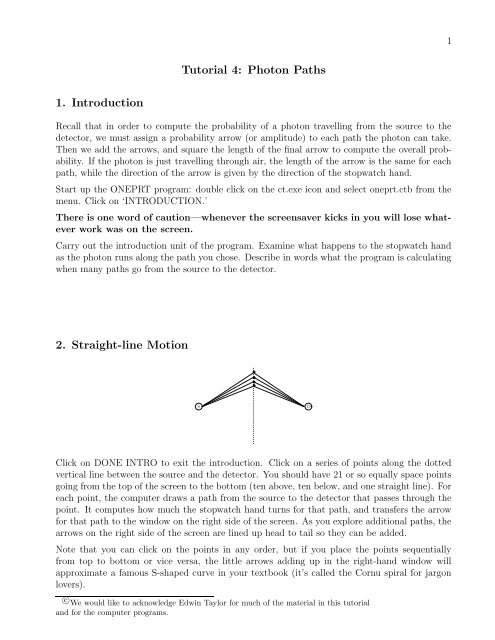
<strong>2.</strong> <strong>Straight</strong>-<strong>line</strong> Motion<br />
S<br />
D<br />
Click on DONE INTRO to exit the introduction. Click on a series of points along the dotted<br />
vertical <strong>line</strong> between the source and the detector. You should have 21 or so equally space points<br />
going from the top of the screen to the bottom (ten above, ten below, and one straight <strong>line</strong>). For<br />
each point, the computer draws a path from the source to the detector that passes through the<br />
point. It computes how much the stopwatch hand turns for that path, and transfers the arrow<br />
for that path to the window on the right side of the screen. As you explore additional paths, the<br />
arrows on the right side of the screen are <strong>line</strong>d up head to tail so they can be added.<br />
Note that you can click on the points in any order, but if you place the points sequentially<br />
from top to bottom or vice versa, the little arrows adding up in the right-hand window will<br />
approximate a famous S-shaped curve in your textbook (it’s called the Cornu spiral for jargon<br />
lovers).<br />
c○ We would like to acknowledge Edwin Taylor for much of the material in this tutorial<br />
and for the computer programs.
<strong>Physics</strong> 008—<strong>Tutorial</strong> 4: <strong>Photon</strong> <strong>Paths</strong> 2<br />
Note that if you make a mistake, then just click again on the midpoint of the mistaken path,<br />
and it will be erased.<br />
Click on the ‘RESULTING ARROW’ button to see the final arrow. The overall probability that<br />
the photon will travel from S to D along these paths is equal to the square of the length of the<br />
final arrow.<br />
<strong>1.</strong> Two students, Daria and Quinn, are discussing this computer experiment.<br />
– Daria: Each arrow has the same length, but their direction matters in finding the total<br />
probability. Some arrows tend to cancel others when you <strong>line</strong> them up, and the final<br />
arrow is not necessarily 21 times the length of the individual arrows.<br />
– Quinn: Nuh uh Daria. Each arrow is the same length. Therefore each path contributes<br />
the same amount to the final arrow. If there are 21 paths, the length of the final arrow<br />
will be 21 times the length of each individual arrow.<br />
With which (if either) of the students do you agree and why?<br />
If we are adding twenty-one arrows each of length L, what is the maximum possible length<br />
for the final arrow? What is the minimum possible length for the final arrow?<br />
<strong>2.</strong> Which paths contribute the most to the final arrow on the right side of the screen? (Repeat<br />
the construction as many times as needed to answer this question.)<br />
3. Use the stopwatch model to explain why those particular paths give a sizable contribution<br />
to the final arrow. (You will need to draw some kind of diagram to explain this.)<br />
Click on ‘ADD DETECTORS.’ The final arrow is copied from the right-hand window to the<br />
position of the original detector. Now click on a point near the top of the screen that lies on the<br />
vertical <strong>line</strong> passing through the original detector.<br />
4. For this new detector, do the paths that contribute significantly to the final arrow pass<br />
through the same midpoints as those that contributed the most for the original detector?<br />
Explain why or why not.
<strong>Physics</strong> 008—<strong>Tutorial</strong> 4: <strong>Photon</strong> <strong>Paths</strong> 3<br />
3. Narrow and Wide Slits<br />
Click on ‘NEW CASE.’ Place five points very close to each other along the vertical dotted <strong>line</strong>,<br />
centered between S and D. This mimics light passing through a narrow slit.<br />
S<br />
D<br />
Press the ‘ADD DETECTORS’ button and click on different locations along the dotted vertical<br />
<strong>line</strong> passing through the original detector. For each new detector location, the final arrow in the<br />
right-hand window is copied to the position of the detector. You can use the ‘CLEAR PATHS’<br />
button to redraw the final arrows for each detector without showing the paths. Include a detector<br />
near the bottom of the screen.<br />
<strong>1.</strong> With a ruler, measure on the screen the lengths of the final arrows for the central detector<br />
and for the detector near the bottom of the screen. Calculate the ratio of the arrow lengths:<br />
(Length of arrow) bottom<br />
(Length of arrow) center<br />
=<br />
<strong>2.</strong> What is the corresponding ratio of the probabilities for detecting photons at the two locations?<br />
Prob.(detection at bottom)<br />
Prob.(detection at center) =<br />
Now let’s mimic a wider slit. Press ‘NEW CASE’ to clear the screen. Now place nine closely<br />
spaced points along the center vertical <strong>line</strong>. (This slit should be about twice the size of the<br />
narrow one above.)<br />
Place additional detectors above and below the original one.<br />
3. With a ruler, measure on the screen the lengths of the final arrows for the central detector<br />
and for the detector near the bottom of the screen. Calculate the ratio of the arrow lengths:<br />
(Length of arrow) bottom<br />
(Length of arrow) center<br />
=<br />
4. What is the corresponding ratio of the probabilities for detecting photons at the two locations?<br />
Prob.(detection at bottom)<br />
Prob.(detection at center) =<br />
5. For both the narrow and wide slits, make a plot (on the next page) of the probability for<br />
detecting a photon as a function of detector location.
<strong>Physics</strong> 008—<strong>Tutorial</strong> 4: <strong>Photon</strong> <strong>Paths</strong> 4<br />
Probability of detecting photon<br />
narrow slit<br />
Detector location<br />
Probability of detecting photon<br />
wide slit<br />
Detector location<br />
4. Two-Slit Interference<br />
Start a ‘NEW CASE.’ Create two very narrow slits by placing two sets of three closely spaced<br />
dots along the central vertical <strong>line</strong>. Put your two slits about equal distance above and below the<br />
central horizontal <strong>line</strong> (put the edge 4 dots above and below the center <strong>line</strong>).<br />
Use ‘ADD DETECTOR’ to examine what happens at locations above and below the original<br />
detector.<br />
S<br />
D<br />
<strong>1.</strong> Find a location above or below the original detector where there is essentially no probability<br />
of detecting a photon.<br />
Sketch the arrows corresponding to the three paths going through the lower slit. Draw the<br />
arrow found by adding these three arrows.<br />
Sketch the arrows corresponding to the three paths going through the upper slit. Draw the<br />
arrow found by adding these three arrows.<br />
How do the arrows for the lower and upper slits compare?<br />
<strong>2.</strong> Sketch (on the next page) how the probability for detecting a photon varies with detector<br />
location.
<strong>Physics</strong> 008—<strong>Tutorial</strong> 4: <strong>Photon</strong> <strong>Paths</strong> 5<br />
Probability of detecting photon<br />
center<br />
Detector location<br />
Start a ‘NEW CASE.’ Now we will increase the separation between the slits. Create two very<br />
narrow slits by placing two sets of three closely spaced dots along the central vertical <strong>line</strong>. Put<br />
your two slits about equal distance above and below the central horizontal <strong>line</strong> (now place them<br />
9 dots above and below the center).<br />
Use ‘ADD DETECTOR’ to examine what happens at locations above and below the original<br />
detector.<br />
3. Find a location above or below the original detector where there is essentially no probability<br />
of detecting a photon.<br />
4. Sketch how the probability for detecting a photon varies with detector location.<br />
Probability of detecting photon<br />
center<br />
Detector location
<strong>Physics</strong> 008—<strong>Tutorial</strong> 4: <strong>Photon</strong> <strong>Paths</strong> 6<br />
5. Explain in your own words what the difference is between these two curves. Use the<br />
quantum model developed in class to explain why this difference occurs.