PEBBLES Mechanics Simulation Speedup - Idaho National Laboratory

INL/CON-09-17136 

PREPRINT 

PEBBLES Mechanics 

Simulation Speedup 

PHYSOR 2010 

Joshua J. Cogliati 

Abderrafi M. Ougouag 

May 2010 

This is a preprint of a paper intended for publication in a journal or 

proceedings. Since changes may be made before publication, this 

preprint should not be cited or reproduced without permission of the 

author. This document was prepared as an account of work 

sponsored by an agency of the United States Government. Neither 

the United States Government nor any agency thereof, or any of 

their employees, makes any warranty, expressed or implied, or 

assumes any legal liability or responsibility for any third party’s use, 

or the results of such use, of any information, apparatus, product or 

process disclosed in this report, or represents that its use by such 

third party would not infringe privately owned rights. The views 

expressed in this paper are not necessarily those of the United 

States Government or the sponsoring agency.

PHYSOR 2010 - Advances in Reactor Physics to Power the Nuclear Renaissance 

Pittsburgh, Pennsylvania, USA, May 9-14, 2010, on CD-ROM, American Nuclear Society, LaGrange Park, IL (2010) 

PEBBLES MECHANICS SIMULATION SPEEDUP 

Joshua J. Cogliati and Abderrafi M. Ougouag 

Idaho National Laboratory 

P.O. Box 1625 

Idaho Falls, ID 83415 

Joshua.Cogliati@inl.gov; Abderrafi.Ougouag@inl.gov 

ABSTRACT 

Pebble bed reactors contain large numbers of spherical fuel elements arranged randomly. 

Determining the motion and location of these fuel elements is useful for calculating certain 

operating parameters of pebble bed reactors. These simulations involve determining the entire core 

motion as hundreds of thousands of pebbles are recirculated over months to years of physical time. 

Single processor algorithms are insufficient for this simulation because they would take decades to 

centuries of wall-clock time. This paper describes the process of parallelizing and speeding up the 

PEBBLES mechanics simulation code. Shared memory programming with the Open 

Multiprocessing Application Programming Interface and distributed memory programming with 

the Message Passing Interface are used simultaneously in this process. A new shared memory 

lock-less linear time collision detection algorithm is described, a method that allows faster 

detection of pebbles in contact than generic methods. This paper also provides an overview of the 

computationally expensive portions of computer codes and the different areas to be optimized. 

These improvements to PEBBLES combine to make full simulations of recirculations in German 

AVR-sized reactors possible in months of wall clock time. 

Key Words: PBR, parallel DEM simulation 

1. INTRODUCTION 

The graphite moderated and helium cooled pebble bed reactor is a leading contender for future 

production of high temperature process heat and electricity. Fuel for this reactor design is 

contained inside of TRISO particles which in turn are contained inside of graphite spheres 

(pebbles) that circulate through the reactor. Fresh fuel pebbles added to the top of the reactor 

vessel travel via gravity to the bottom of the reactor where they are either removed or recirculated, 

depending on their measured burn-up. 

Understanding and optimizing the operation of a pebble bed reactor requires determining the flow 

and average properties of the pebbles. The neutrons in graphite have longer mean free paths than 

in light water reactors, so exact positional details are less important, but bulk properties, such as 

average density, flow, and organization patterns, need to be understood. Being able to determine 

these type of characteristics was the direct motivation for the creation of the PEBBLES 

mechanics code. This code simulates each individual pebble with a discrete element method. The 

forces on each pebble are calculated and the calculations are used to simulate their subsequent 

motion. This simulation has multiple applications. 

In simulating the neutronics, typical pebble locations need to be determined so that accurate 

Dancoff factors can be calculated[1]. The PEBBLES code can calculate the velocity profile


across the reactor during recirculation. The velocity profile can then be used to determine the 

asymptotic behavior of the reactor using the PEBBED neutronics code. A bed of pebbles can be 

created and then shaken using the motion data for an earthquake[2] which can provide 

densification data for simulation of the neutronic effect of an earthquake. If accurate graphite 

wear coefficients are available, PEBBLES can be used for calculating the dust production of the 

reactor bed as it recirculates[3]. Optimizing the speed of the code is vital for all these uses. 

The PEBBLES program has three major portions of calculation: the first determines which 

pebbles are in contact with other pebbles, the second computes the time derivatives for all the 

vectors for all the pebbles, and the third computes the derivatives to update the values. Overall, 

the algorithm’s computation time for calculation of a single time step is linearly proportional to 

the number of pebbles, that is O(n). 

2. GENERAL INFORMATION ABOUT PROFILING 

The complete calculation has the following four different generic parts that need to be considered 

in determining the overall speed: 

1. The first consideration is the time it takes to compute arithmetic operations. Modern 

processors can complete arithmetic operations in nanoseconds or fractions of nanoseconds. 

In the PEBBLES code, the amount of time spent on arithmetic is practically undetectable in 

wall clock changes. 

2. The second consideration is the time to read and write memory. This takes hundreds of CPU 

clock cycles for main memory access, so these times are on the order of fractions of 

microseconds[4]. Because of the time required to access main memory, all modern CPUs 

have on chip caches that contain a copy of the recently used memory. If the memory access 

is in the CPU’s cache, the memory can be retrieved and written in a small number of CPU 

cycles. Main memory writes are somewhat more expensive than main memory reads, since 

any copies of the memory that exist in other processor’s caches need to be updated or 

invalidated. So for a typical calculation like a + b → c the time spent on the arithmetic is 

trivial compared to the time spent reading in a and b and writing out c. 

3. The third consideration is the amount of time required for parallel programming constructs. 

Various parallel synchronization tools such as atomic operations, locks, and critical sections 

take an amount of time on the same order of magnitude as memory writes. However, they 

typically need a read and then a write without any other processor being able to access that 

chunk of memory in between. This requires additional overhead and a possible wait if the 

memory address is being used by another process. Atomic operations on x86 64 

architectures are faster than using locks, and locks are generally faster than using OpenMP 

critical sections. 

4. The fourth consideration is network time. Sending and receiving a value can easily take over 

a millisecond for the round trip time. 

These four time-consuming operations need to be considered when choosing algorithms and 

methods of calculation. 


Pittsburgh, Pennsylvania, USA, May 9-14, 2010 

2/11

PEBBLES Mechanics Simulation Speed-up 

There are a variety of methods for profiling the computer code. The simplest method is to use the 

FORTRAN 95 intrinsics CPU TIME and DATE AND TIME. The CPU TIME subroutine returns a 

real number of seconds of CPU time. The DATE AND TIME subroutine returns the current wall 

clock time in the VALUES argument. With gfortran, both these times are accurate to at least a 

millisecond. The difference between two different calls of these functions provide information on 

both the wall clock time and the CPU time between the calls. (For the DATE AND TIME 

subroutine, it is easiest if the days, hours, minutes, seconds, and milliseconds are converted to real 

seconds past some arbitrary time.) The time methods provide basic information and a good 

starting point for determining which parts of the program are consuming time. For more detailed 

profiling the oprofile[5] program can be used on Linux. This program can provide data at the 

assembly language level that makes it possible to determine which part of a complex function is 

consuming the time. Non-assembly language profilers are difficult to accurately use on optimized 

code, and profiling non-optimized code is misrepresentative. 

3. OVERVIEW OF PARALLEL ARCHITECTURES AND CODING 

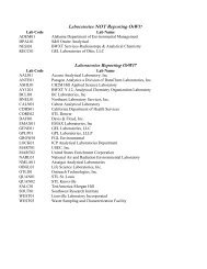
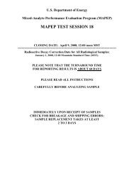
Parallel computers can be arranged in a variety of ways. Because of the expense of linking shared 

memory to all processors, a common architecture is a cluster of nodes with each node having 

multiple processors. Each node is linked to other nodes via a fast network connection. The 

processors on a single node share memory. Figure 1 shows this arrangement. For this 

arrangement, the code can use both the OpenMP (Open Multi-Processing)[6] and the MPI 

(Message Passing Interface)[7] libraries. OpenMP is a shared memory programming interface 

and MPI is a programming interface for transferring data across a network to other nodes. By 

using both programming interfaces, high speed shared memory accesses can be used and the code 

can be parallelized across multiple nodes. 

 

 

 

 

 

 

 

 

 

 

 

 

 

 

 

 

 

 

 

 

 

 

 

 

 

 

 

 

Figure 1. Sample Cluster Architecture 

4. OVERVIEW OF PEBBLES COMPUTATION 

The PEBBLES simulation tracks each individual pebble’s velocity, position, angular velocity, and 

static friction loadings. The following classical mechanics differential equations are used for 

calculating the time derivatives of the first three variables. The computation of the static friction 

loading derivative is more extensive and described in a companion paper. 



3/11


dv i 

dt = m ig + ∑ i≠j F ij + F ci 

m i 

(1) 

dp i 

dt = v i (2) 

∑ 

dω i 

dt = i≠j F ‖ij × r iˆn ij + F ‖ci × r iˆn ci 

(3) 

I i 

ds ij 

= S(F ⊥ij , v i , v j , p i , p j , s ij ) (4) 

dt 

where F ij is the force from pebble j on pebble i, F ci is the force of the container on pebble i, g is 

the gravitational acceleration constant, m i is the mass of pebble i, v i is the velocity of pebble i, p i 

is the position vector for pebble i, ω i is the angular velocity of pebble i, F ‖ij is the tangential force 

between pebbles i and j, F ⊥ij is the perpendicular force between pebbles i and j, r i is the radius 

of pebble i, I i is the moment of inertia for pebble i, F ‖ci is the tangential force of the container on 

pebble i, ˆn ci is the unit vector normal to the container wall on pebble i, ˆn ij is the unit vector 

pointing from the position of pebble i to that of pebble j, s ij is the current static friction loading 

between pebbles i and j, and S is the function to compute the change in the static friction loading. 

The static friction model contributes to the F ‖ij term which is also part of the F ij term. 

The main loop of the single processor version code runs the following steps for each time step 

when computing the derivatives using the Euler method: 

1. Calculates which pebbles are near each other. 

2. Computes the derivatives of the velocity, position, angular velocity, and static friction 

loadings. 

3. Applies the derivatives to determine the next velocity, position, angular velocity, and static 

friction loadings. 

For the single processor version, PEBBLES allows other methods of computing the next time step 

including Runge-Kutta and Adams-Moulton. At present, these have not allowed substantially 

smaller time steps to be used. The Runge-Kutta method was tried experimentally with MPI, but 

the additional data transfer required (since pebbles can effect more than just their immediate 

neighbor) more than offset the gain of using the method resulting in a slowdown. 

Simulation time steps of 0.1 ms are used for the Euler method computation. This small time step 

is required to prevent two pebbles from going from noncontacting in one time step to contacting 

with enough overlap that the Hooke’s law force produces a substantial energy gain in the next 

time step. Larger time steps are possible if a weaker Hooke’s law force is used, but that results in 

‘squishy’ pebbles, and larger overlaps between pebbles. The Hooke’s law force in PEBBLES is 

chosen to keep overlaps between pebbles under a millimeter. However, because small time steps 



4/11


are being used, simulation of hundreds of thousands of pebbles being recirculated requires very 

large numbers of simulated time steps. This workload might be able to be reduced by reducing 

the number of pebbles simulated (such as by only simulating a vertical third of the reactor), or by 

only simulating a partial recirculation. 

5. LOCK-LESS PARALLEL O(N) COLLISION DETECTION 

For any granular simulation, which particles are in contact needs to be determined quickly and 

accurately for each time step. This is referred to as collision detection, though it might more 

accurately be labeled contact detection for pebble simulations. The naive algorithm for collision 

detection is to iterate over all the other objects and compare each of them to the current object for 

collision. However, O(N 2 ) time is required determine all the collisions using that method. An 

improved algorithm by Cohen et al. uses six sorted lists of the lower and upper bounds for each 

object. (there is one upper bound list and one lower bound list for each dimension.) Determining 

the collisions for a given object with this algorithm requires the bounds of the current objects to 

be compared to bounds in the list—only objects that overlap the bounds in all three dimensions 

can potentially be colliding. This algorithm typically has approximately O(Nlog(N)) time, 

because of the sorting of the bounding lists[8]. 

An alternative faster method is available for simulations such as a pebble bed simulation because 

the following requirements hold: (1) there is a maximum diameter of object, and no object 

exceeds this diameter, and (2) for a given volume, there is a reasonably small finite maximum 

number of objects that could ever be in that volume. These two constraints are easily satisfied by 

pebble bed simulations, since the pebbles are effectively the same size (small changes in diameter 

occur due to wear and thermal effects). For this case, the grid collision detection method can be 

used. A three-dimensional parallelepiped grid is used over the entire range that the pebbles are 

simulated. The grid spacing gs is set at the maximum diameter of any object (twice the maximum 

radius for spheres). 

Two key variables are initialized: grid count(x, y, z) which are the number of pebbles in grid 

locations x,y,z, and grid ids(x, y, z, i) which are the pebble identification numbers (ids) for each 

x,y,z location. The id is a unique number assigned to each pebble in the simulation. The spacing 

between successive grid indexes is gs, so the index of a given x location can be determined by 

⌊(x − x min )/gs⌋ where x min is the zero x index’s floor; similar formulas are used for y and z. 

The grid is initialized by setting grid count(:, :, :)=0, and then the x,y,z indexes are determined 

for each pebble. The grid count at that location is then atomically incremented by one and 

fetched. Because OpenMP 3.0 does not have a atomic add-and-fetch, the lock xadd x86 64 

assembly language instruction is used in a function. The grid count provides the fourth index 

into the grid ids array, so the pebble id can be stored into the ids array. The iteration over the 

pebbles can be done in parallel because of the use of an atomic add-and-fetch function. The 

amount of time to zero the grid count array is a function of the volume of space, which is 

proportional to the number of pebbles. Updating the grid iterates over the entire list of pebbles so 

the full algorithm for updating the grid is O(N) for the number of pebbles. 

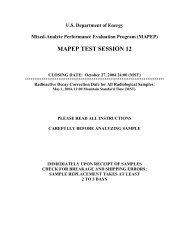
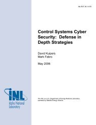
Once the grid is updated, the nearby pebbles can be quickly determined. Figure 2 illustrates the 

general process. First, indexes values are computed from the pebble and used to generate xc,yc, 



5/11


and zc. This finds the center grid location, which is shown as the highlighted box in the figure. 

Then, all the possible pebble collisions must have grid locations (that is their centers are in the 

grid locations) in the dotted box, which can be found by iterating over the grid locations from 

xc − 1 to xc +1and repeated for the other two dimensions. There are 3 3 grid locations to check, 

and the number of pebbles in them are bounded (maximum 8), so the time to do this is bounded. 

Since this does not change any grid values, it can be done in parallel without any locks. 

 

 

Figure 2. Determining Nearby Pebbles from Grid 

Therefore, because of the unique features of pebble bed pebbles simulation, a parallel lock-less 

O(N) algorithm for determining the pebbles in contact can be created. 

6. MPI SPEEDUP 

The PEBBLES code uses MPI to distribute the computational work across different nodes. The 

MPI/OpenMP hybrid parallelization splits the calculation of the derivatives and the new variables 

geometrically and passes the data at the geometry boundaries between nodes using messages. 

Each pebble has a primary node and may also have various boundary nodes. The pebble primary 

node is responsible for updating the pebble position, velocity, angular velocity, and slips. The 

pebble primary node also sends data about the pebble to any nodes that are the pebble boundary 

nodes and will transfer the pebble to a different node if the pebble crosses the geometric boundary 

of the node. Boundary pebbles are those close enough to a boundary that their data needs to be 

present in multiple nodes so that the node’s primary pebbles can be properly updated. Node 0 is 

the master node and does processing that is simplest to do on one node, such as writing restart 

data to disk and initializing the pebble data. The following steps are used for initializing the nodes 

and then transferring data between them: 

1. Node 0 calculates or loads initial positions of pebbles. 

2. Node 0 creates the initial domain to node mapping. 

3. Node 0 sends domain to node mapping to other nodes. 

4. Node 0 sends other nodes their needed pebble data. 



6/11


Order of calculation and data transfers in main loop: 

1. Calculate derivatives for node primary and boundary pebbles. 

2. Apply derivatives to node primary pebble data. 

3. For every primary pebble, check with the domain module to determine the current primary 

node and any boundary nodes. 

(a) If the pebble now has a different primary node, add the pebble id to the transfer list to 

send to the new primary node. 

(b) If the pebble has any boundary nodes, add the pebble id to the boundary send list to 

send it to the node for which it is a boundary. 

4. If this is a time step where Node 0 needs all the pebble data (such as when restart data is 

being written), add all the primary pebbles to the Node 0 boundary send list. 

5. Send the number of transfers and the number of boundary sends that this node has to all the 

other nodes using buffered sends. 

6. Initialize three Boolean lists of other nodes that this node has: 

(a) data to send to with “true” if the number of transfers or boundary sends is nonzero, and 

“false” otherwise 

(b) received data from to “false” 

(c) received the number of transfers and the number of boundary sends with “false.” 

7. While this node has data to send to other nodes and other nodes have data to send to this 

node loop: 

(a) Probe to see if any nodes that this node needs data from have data available. 

i. If yes, then receive the data and update pebble data and the Boolean lists as 

appropriate 

(b) If there are any nodes that this node has data to send to, and this node has received the 

number of transfers and boundary sends from, then send the data to those nodes and 

update the Boolean data send list for those nodes. 

8. Flush the network buffers so any remaining data gets received. 

9. Node 0 calculates needed tallies. 

10. If this is a time to rebalance the execution load: 

(a) Send wall clock time spent computing since last rebalancing to node 0 

(b) Node 0 uses information to adjust geometric boundaries to move work towards nodes 

with low computation time and away from nodes with high computation time 

(c) Node 0 sends new boundary information to other nodes, and needed data to other nodes. 

11. Continue to next time step and repeat this process. 



7/11


All the information and subroutines needed to calculate the primary and boundary nodes that a 

pebble belongs to are calculated and stored in a FORTRAN 95 module named 

network domain module. The module uses two derived types: network domain type 

and network domain location type. Both types have no public components so the 

implementation of the domain calculation and the location information can be changed without 

changing anything but the module. The location type stores the primary node and the boundary 

nodes of a pebble. The module contains subroutines for determining the location type of a pebble 

based on its position, primary and boundary nodes for a location type, and subroutines for 

initialization, load balancing, and transferring of domain information over the network. The 

internals of the module can be changed without changing the rest of the PEBBLES code. The 

current method of dividing the nodes into geometric domains uses a list of boundaries between 

the z (axial) locations. This list is searched via binary search to find the nodes nearest to the 

pebble position, as well as those within the boundary layer distance above and below the zone 

interface in order to identify all the boundary nodes that participate in data transfers. The location 

type resulting from this is cached on a fine grid, and the cached value is returned when the 

location type data is needed. The module contains a subroutine that takes a work parameter 

(typically the computation time of each of the nodes) and can redistribute the z boundaries to shift 

work towards nodes that are taking less time computing their share of information. If needed in 

the future, the z-only method of dividing the geometry could be replaced by a full 3-D version by 

modifying the network domain module. 

7. OPENMP SPEEDUP 

The PEBBLES code uses OpenMP to distribute the calculation over multiple processes on a 

single node. OpenMP allows directives to be given to the compiler that direct how portions of 

code are to be parallelized. This allows a single piece of code to be used for both the single 

processor version and the OpenMP version. The PEBBLES parallelization typically uses 

OpenMP directives to cause loops that iterate over all the pebbles to be run in parallel. Some 

details need to be taken into consideration for the parallelization of the calculation of acceleration 

and torque. The physical accelerations imposed by the wall are treated in parallel, and there is no 

problem with writing over the data because each processor is assigned a portion of the total zone 

inventory of pebbles. For calculating the pebble-to-pebble forces, each processor is assigned a 

fraction of the pebbles, but there is a possibility of the force addition computation overwriting 

another calculation because the forces on a pair of pebbles are calculated and then the calculated 

force is added to the force on each pebble. In this case, it is possible for one processor to read the 

current force from memory and add the new force from the pebble pair while another processor is 

reading the current force from memory and adding its new force to that value; they could both 

then write back the values they have computed. This would be incorrect because each calculation 

has only added one of the new pebble pair forces. Instead, PEBBLES uses an OpenMP ATOMIC 

directive to force the addition to be performed atomically, thereby guaranteeing that the addition 

uses the latest value of the force sum and saves it before a different processor has a chance to read 

it. For calculating the sum of the derivatives using Euler’s method, updating concurrently poses 

no problem because each individual pebble has derivatives calculated. The data structure for 

storing the pebble-to-pebble slips (sums of forces used to calculate static friction) is similar to the 

data structure used for the collision detection grid. A 2-D array exists where one index is the 

from-pebble and the other index is for storing ids of the pebbles that have slip with the first 



8/11


pebble. A second array exists that contains the number of ids stored, and that number is always 

added and fetched atomically, which allows the slip data to be updated by multiple processors at 

once. These combine to allow the program to run efficiently on shared memory architectures. 

8. CHECKING THE PARALLELIZATION 

The parallelization of the algorithm is checked by running the test case with a short number of 

time steps (10 to 100). Various summary data are checked to make sure that they match the values 

computed with the single processor version and between different numbers of nodes and 

processors. For example, with the NGNP-600 model used in the results section, the average 

overlap of pebbles at the start of the run is 9.66528090546041503E-005 meters. The single 

processor average overlap at the end of the 100 time-step run is 9.69305722615893206E-005 

meters, the 2 nodes average overlap is 9.69304304673814892E-005 meters, and the 12 node 

average overlap is 9.69302936897353682E-005 meters. The lower order numbers change from 

run to run. The start-of-run values match each other exactly, and the end-of-run values match the 

start of run values to two significant figures. However, the three different end-of-run values match 

to five significant digits. In short, the end values match each other much closer than they match 

the start values. The overlap is very sensitive to small changes in the calculation because it is a 

function of the difference between two positions. During coding, multiple defects were found and 

corrected by checking that the overlaps matched close enough between the single processor 

calculation and the multiple processor calculations. The total energy or the linear energy or other 

computations can be used similarly since the lower significant digits also change frequently and 

are computed over all the pebbles. 

9. RESULTS 

The data in Table I and Table II provide information on the time used with the current version of 

PEBBLES for running 80 simulation time steps on two models. The NGNP-600 model has 

480,000 pebbles. The AVR model contains 100,000 pebbles. All times are reported in units of 

wall-clock seconds. The single processor NGNP-600 model took 251.054 seconds and the AVR 

single processor model took 47.884 seconds when running the current version. The timing runs 

were carried out on a cluster with two Intel Xeon X5355 2.66 GHz processors per node with a 

DDR 4X InfiniBand interconnect network. The gfortran 4.3 compiler was used. 

Significant speedups have resulted with both the OpenMP and MPI/OpenMP versions. A basic 

time step for the NGNP-600 model went from 3.138 seconds to 146 milliseconds when running 

on 64 processors. Since a full recirculation would take on the order of 1.6e9 time steps, the wall 

clock time for running the simulations has gone from about 160 years to a little over 7 years. For 

smaller simulation tasks, such as simulating the motion of the pebbles in a pebble bed reactor 

during an earthquake, the times are more reasonable taking about 5e5 time steps. Thus, for the 

NGNP-600 model, a full earthquake can be simulated in about 20 hours when using 64 

processors. For the smaller AVR model, the basic time step takes about 34 milliseconds when 

using 64 processors. Since there are less pebbles to recirculate, a full recirculation would take on 

the order of 2.5e8 time steps, or about 98 days of wall clock time. 



9/11


Table I. OpenMP speedup results 

Processes AVR Speedup Efficiency NGNP-600 Speedup Efficiency 

1 47.884 1 100.00% 251.054 1 100.00% 

1 53.422 0.89633 89.63% 276.035 0.90950 90.95% 

2 29.527 1.6217 81.09% 152.479 1.6465 82.32% 

3 21.312 2.2468 74.89% 104.119 2.4112 80.37% 

4 16.660 2.8742 71.85% 80.375 3.1235 78.09% 

5 13.884 3.4489 68.98% 68.609 3.6592 73.18% 

6 12.012 3.98635 66.44% 61.168 4.1043 68.41% 

7 10.698 4.4760 63.94% 54.011 4.6482 66.40% 

8 9.530 5.0246 62.81% 49.171 5.1057 63.82% 

Table II. MPI/OpenMP speedup results 

Nodes Processes AVR Speedup Efficiency NGNP-600 Speedup Efficiency 

1 1 47.884 1 100.00% 251.054 1 100.00% 

1 8 10.696 4.4768 55.96% 55.723 4.5054 56.32% 

2 16 6.202 7.7207 48.25% 30.642 8.1931 51.21% 

3 24 4.874 9.8244 40.93% 23.362 10.746 44.78% 

4 32 3.935 12.169 38.03% 17.841 14.072 43.97% 

5 40 3.746 12.783 31.96% 16.653 15.076 37.69% 

6 48 3.534 13.550 28.23% 15.928 15.762 32.84% 

7 56 3.285 14.577 26.03% 15.430 16.271 29.05% 

8 64 2.743 17.457 27.28% 11.688 21.480 33.56% 

9 72 2.669 17.941 24.92% 11.570 21.699 30.14% 

10 80 2.657 18.022 22.53% 11.322 22.174 27.72% 

11 88 2.597 18.438 20.95% 11.029 22.763 25.87% 

12 96 2.660 18.002 18.75% 11.537 21.761 22.67% 

10. CONCLUSIONS 

The PEBBLES code has been sped up to the point where full recirculations in AVR sized reactor 

can be simulated. The projected calculation time for the NGNP-600 full recirculation simulation 

has gone from over a century to under a decade, which is approaching practical lengths. Potential 

algorithm, processor, and memory speed improvements may make full recirculations more 

possible in the near future. 

11. ACKNOWLEDGMENTS 

This work was supported by the U.S. Department of Energy, Assistant Secretary for the office of 

Nuclear Energy, under DOE Idaho Operations Office Contract DEAC07-05ID14517. 



10/11


REFERENCES 

[1] A. M. Ougouag, J. J. Cogliati, and J-L Kloosterman, “Methods of Modeling the Packing of 

Fuel Elements in Pebble Bed Reactors,” Mathematics and Computation, Supercomputing, 

Reactor Physics and Nuclear and Biological Applications Avignon, France, September 

12–15, American Nuclear Society, (2005). 

[2] A. M. Ougouag, J. Ortensi, and H. Hiruta, “Analysis of an Earthquake-Initiated-Transient 

in a PBR,” International Conference on Mathematics, Computational Methods & Reactor 

Physics, Saratoga Springs, New York, May 3–7, (2009). 

[3] J. J. Cogliati and A. M. Ougouag, “Pebble Bed Reactor Dust Production Model,” 

Proceedings of the 4th International Topical Meeting on High Temperature Reactor 

Technology, Washington, D.C., USA, September 28 – October 1, (2008). 

[4] Ulrich Drepper, “What Every Programmer Should Know About Memory,” 

http://people.redhat.com/drepper/cpumemory.pdf (2007) 

[5] “OProfile - A System Profiler for Linux,” http://oprofile.sourceforge.net (2009) 

[6] “OpenMP Application Program Interface, Version 3.0” 

http://www.openmp.org/mp-documents/spec30.pdf (2008) 

[7] “MPI: A Message-Passing Interface Standard, Version 2.2,” 

http://www.mpi-forum.org/docs/mpi-2.2/mpi22-report.pdf (2009) 

[8] Jonathan D. Cohen, Ming C. Lin, Dinesh Manocha, and Madhav K. Ponamgi, 

“ICOLLIDE: an Interactive and Exact Collision Detection System for Large Scale 

Environments,” Proceedings of the 1995 Symposium on Interactive 3D Graphics, 

Monterey, CA, April 9-12, 1995, pp. 19-24 



11/11

PEBBLES Mechanics Simulation Speedup - Idaho National Laboratory

Create successful ePaper yourself

Delete template?

Save as template?