CALCULATOR EXERCISES - School of Information - The University ...

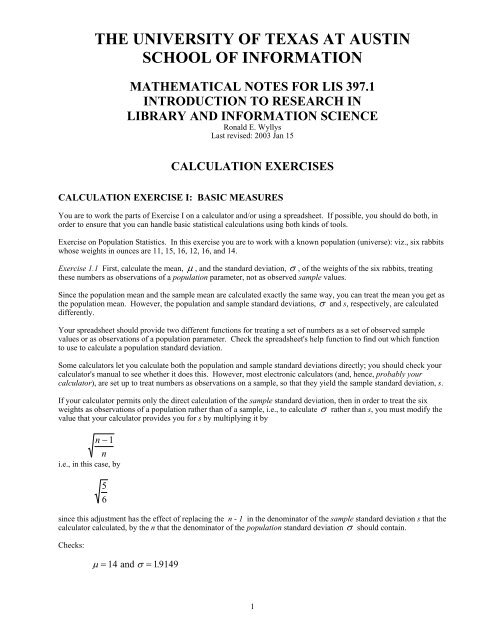
THE UNIVERSITY OF TEXAS AT AUSTIN
SCHOOL OF INFORMATION
MATHEMATICAL NOTES FOR LIS 397.1
INTRODUCTION TO RESEARCH IN
LIBRARY AND INFORMATION SCIENCE
Ronald E. Wyllys
Last revised: 2003 Jan 15
CALCULATION EXERCISES
CALCULATION EXERCISE I: BASIC MEASURES
You are to work the parts of Exercise I on a calculator and/or using a spreadsheet. If possible, you should do both, in
order to ensure that you can handle basic statistical calculations using both kinds of tools.
Exercise on Population Statistics. In this exercise you are to work with a known population (universe): viz., six rabbits
whose weights in ounces are 11, 15, 16, 12, 16, and 14.
Exercise 1.1 First, calculate the mean, µ , and the standard deviation, σ , of the weights of the six rabbits, treating
these numbers as observations of a population parameter, not as observed sample values.
Since the population mean and the sample mean are calculated exactly the same way, you can treat the mean you get as
the population mean. However, the population and sample standard deviations, σ and s, respectively, are calculated
differently.
Your spreadsheet should provide two different functions for treating a set of numbers as a set of observed sample
values or as observations of a population parameter. Check the spreadsheet's help function to find out which function
to use to calculate a population standard deviation.
Some calculators let you calculate both the population and sample standard deviations directly; you should check your
calculator's manual to see whether it does this. However, most electronic calculators (and, hence, probably your
calculator), are set up to treat numbers as observations on a sample, so that they yield the sample standard deviation, s.
If your calculator permits only the direct calculation of the sample standard deviation, then in order to treat the six
weights as observations of a population rather than of a sample, i.e., to calculate σ rather than s, you must modify the
value that your calculator provides you for s by multiplying it by
n − 1
n
i.e., in this case, by
5
6
since this adjustment has the effect of replacing the n - 1 in the denominator of the sample standard deviation s that the
calculator calculated, by the n that the denominator of the population standard deviation σ should contain.
Checks:
µ = 14 and σ = 19149 .
1

Exercise 1.2 Next, draw five different samples of size 2 from this universe; namely, sample A = 11, 16; B = 15, 12; C
= 11, 12; D = 14, 16; and E = 16, 16. Calculate the sample mean and standard deviation for each sample.
Checks:
A: X = 13.5000; s = 3.5355
B: X = 13.5000; s = 2.1213
C: X = 11.5000; s = 0.7071
D: X = 15.0000; s = 1.4142
E: X = 16.0000; s = 0.0000
Exercise 1.3 Now find (a) the mean of these sample means, and (b) the mean of these sample SDs. How do the results
compare with the population values you found earlier? I.e., how does the mean of these five sample means compare
with the population mean? how does the mean of these five sample SDs compare with the population SD?
Note, first, the variation among the various sample means and SDs. This example is intended to be instructive with
respect to the range of variation possible in sampling, especially with samples of very small size.
Note, second, that the mean of these sample means is closer to the population mean than any of the individual means of
the samples, and that the mean of the sample SDs is closer to the population SD than most of the sample SDs. This
illustrates the general principle that the larger the sample, the closer the sample values tend to be to the corresponding
population parameters.
Checks:
(a) Mean of the five sample means = 13.9000
(b) Mean of the five sample SDs = 1.5556
CALCULATION EXERCISE II: t-TESTS OF HYPOTHESES
You are to work the parts of Exercise II on a calculator and/or using a spreadsheet. If possible, you should do both, in
order to ensure that you can handle basic statistical calculations using both kinds of tools.
This exercise is intended to give you some practice in testing the kind of statistical hypothesis that is concerned with
whether a population mean has a particular value. In reporting your conclusion for each part of this exercise, you
should state an appropriate hypothesis and interpret your result fully; i.e., not only should you say whether your
decision is to reject or not to reject the hypothesis but also you should say what your decision about the truth of the
hypothesis means in terms of the original situation.
Exercise 2.1 You have just graduated from GSLIS and have gone to work in the Catalog Department of a large library.
Being the junior professional in the Department, you have been assigned, among other things, the duty of supervising
the clerks who input cataloging data into the OCLC database. Currently, these clerks work a full 4-hour shift with one
15-minute break in the middle. Full of fresh ideas on personnel management from your GSLIS Administration course
and imbued from your Research course with the idea that "sometimes there is a better way," you wonder whether three
10-minute breaks evenly spaced through the 4-hour shift might change the data-input efficiency, as measured by total
numbers of cataloging records entered per clerk per shift. You know that the current mean number of records entered
per clerk per shift is 127.
You persuade the Head of the Catalog Department to let you try out the new break pattern. In the third week of the
new pattern, when you feel its novelty has worn off enough, you obtain the random sample given below of total
numbers of records entered in one shift by different clerks. You use these data to perform a t-test of the hypothesis that
the mean data-entry rate is still 127 cataloging records per clerk per shift. If you use a 95-percent confidence interval
or--equivalently--work at a 5-percent level of significance, what is your conclusion?
Checks:
104 191 210 169 96 209
199 189 130 204 101 217
X = 168. 2500; s = 46. 9877; s X
= 135642 .
The 95% confidence interval for the population mean is (138.40, 198.10)
2

Exercise 2.2 A little less than a year ago, when your library first started offering a database-searching service to your
patrons, you found that the mean cost to your patrons of a database search was $34.56. Now that it is close to the time
for a decision on whether to renew the contract with the database service, you wonder whether your staff have grown
more skilled in assisting patrons with searches and whether patrons (at least those who use the service repeatedly) have
grown more sophisticated in formulating their search questions. If either or both of these possibilities has occurred,
there ought to be a noticeable decrease in the mean cost of a search.
To investigate, you check the costs of the most recent 40 searches (which you judge to constitute an adequately random
sample), and you obtain the data below. You use these data to perform a t-test of the hypothesis that the mean cost is
still $34.56. If you use a 95-percent confidence interval or--equivalently--work at a 5-percent level of significance,
what is your conclusion?
Checks:
20.47 39.12 37.24 37.43 27.19
14.23 44.80 34.08 38.30 56.28
40.34 38.34 23.14 5.98 49.39
17.72 20.02 50.22 48.83 29.80
28.28 31.96 27.48 41.67 25.31
25.93 43.25 37.62 23.97 28.00
50.25 41.81 41.46 34.57 31.01
15.24 43.91 25.90 32.71 28.97
X = 33. 3055; s = 111951 . ; s X
= 17701 .
The 95% confidence interval for the population mean is (29.73, 36.88)
CALCULATION EXERCISE III: ANOVA AND t-TESTS
This exercise is intended to give you some practice in carrying out the analysis-of-variance (ANOVA) procedure,
together with further practice in using the t-test procedure. Both procedures can be carried by using a calculator and/or
a spreadsheet program and following the arithmetic steps explained in LIS 397.1. However, since even modest
statistical program packages these days contain a module for doing ANOVA, I recommend doing the parts of Exercise
III using such a package.
Exercise 3.1 The following table contains a randomly selected set of actual total GRE scores of GSLIS students. A
naive examination reveals that the men have a higher mean score than the women, and thus seems to suggest that the
men are smarter than the women. But what does a careful examination reveal?
One way of doing a careful examination is apply the ANOVA procedure to these scores. For Exercise 3.1 please use a
calculator to carry out an ANOVA test on the scores. Going through the manual calculation procedure once will help
you understand better the ANOVA tables produced by computer programs that do ANOVA.
Women 1030 1310 1050 1140 1300 1310 720 1140 1020 1160
Men 1210 1230 1570 1090 1230 1010 1300 860 1240 1180
To help you check your arithmetic, here are two entries in the ANOVA table:
T 631,300
B
SS DF MS F
W 33,551.11
State an appropriate hypothesis, and interpret your result fully; i.e., you are not only to say whether your decision is to
reject or not to reject the null hypothesis but also to say what the ANOVA result means in terms of the original
exercise.
Exercise 3.2 With the data given in Exercise 3.1, carry out a test of the appropriate hypothesis by means of the t-test
for independent samples, using the pooled-estimate-of-variance procedure. State your hypothesis, and interpret your
3

esult fully. (If you use Microsoft Excel to work this exercise, you should note that the pooled-estimate-of-variance
procedure is invoked in Excel by using the procedure called "t-Test: Two-Sample Assuming Unequal Variances".)
Checks:
t obs = -0.90337
P(T

Exercise 4.2.2 Also use this sample to test the null hypothesis
Check:
: Detective stories circulate twice as frequently on Saturdays and Sundays as on other days of the week
H 02
2
χ obs
= 2.07
Exercise 4.3 Female vs. Male Library Budgets. The following data are taken from Table 8 of the following article:
Blankenship, W. C. How Many Men? How Many Women? College and Research Libraries. 1967 January; 28:41-8.
PER CENT OF NUMBER OF NUMBER OF
INSTITUTIONAL MALE HEAD FEMALE HEAD
BUDGET LIBRARIANS LIBRARIANS
under 2% 9 6
2-4% 78 60
4-6% 92 109
over 6% 19 18
These data concern the numbers of men and women directors of academic libraries, in a random sample of such
directors, who reported obtaining, for their libraries, budgets expressed as various percentages of the overall budgets of
their colleges or universities. Blankenship says that from these data "It would appear that the ladies are slightly better
at getting the money than are the men."
Do Blankenship's data support his comment? Apply the chi-square test of association to his data. State an appropriate
null hypothesis, work out the observed chi-square score to three decimal places, and interpret the result.
Check:
2
χ obs
= 4.349
CALCULATION EXERCISE V: REGRESSION
You are to work the parts of Exercise V on a calculator and/or using a spreadsheet. If possible, you should do both, in
order to ensure that you can handle basic statistical calculations using both kinds of tools.
This exercise is intended to illustrate some of the ideas of regression analysis. To provide a numerical illustration, we
use the example of an actual study that compared the heights of brothers and sisters to see whether tall sisters tended to
have tall brothers, or equally well put, whether short brothers tended to have short sisters. In this context, of course, a
"tall" sister (brother) is one who is tall compared to the average height for women (men), and similarly for "short"
people.
Here are the data, with heights in inches:
SIBLING PAIR NUMBER
1 2 3 4 5 6 7 8 9 10 11
Brother 71 68 66 67 70 71 70 73 72 65 66
Sister 69 64 65 63 65 62 65 64 66 59 62
Your first step is to plot these observed pairs of points on a page of graph paper or cross-section paper (paper ruled both
horizontally and vertically in increments of, for example, 1/5 or 1/4 inch). Use a scale that not only will be convenient
but also will spread the points over an area of at least 5 or 6 inches both horizontally and vertically. For the sake of
uniformity, it is necessary to make an arbitrary choice of axes and of independent and dependent variables: the sisters'
heights are to be plotted on the horizontal axis, the X-axis, and the brothers' heights on the vertical axis, the Y-axis.
Following the usual (though not mandatory) arrangement, this means that we shall consider the X-axis variable, sister's
height, as the independent variable and, hence, brother's height as the dependent variable.
When you have finished plotting the eleven points, try sketching (i.e., drawing free-hand) a straight line that seems to
you to represent the overall tendency of siblings to have comparable heights (with respect to the mean height of each
sibling's sex). In other words, sketch a straight line that seems to you to represent the overall trend of the plotted
points. You may find it helpful to use a transparent ruler in drawing this line. (Note: You can do the plotting of the
5

points via a spreadsheet, but I want you to do, by hand and eye judgment alone (with the aid of a rulef), the drawing of
a straight line through the points after you have printed out the plotted points.)
Next, either (a) by employing computational formulas from the LIS 397.1 Website Mathematical Note on "Using Regression
to Estimate and Predict," or (b) by using formulas from your text, or (c) by means of the regression function in
your calculator or spreadsheet, you are to calculate the regression coefficients: B 0 , the intercept coefficient; and B 1 , the
slope coefficient. Write out the regression equation, putting the numerical values you find into the basic equation
!
Y = B + B X
0 1
Pick any two values for X that are within the range of the observed values of sisters' heights, preferably two values that
are well separated (e.g., 62 and 69 inches). Calculate the predicted values of Y that correspond to the X values you
chose, and plot these predicted values on your chart. They are two points on the regression line, and as such, they are
sufficient to define this line. With a ruler, draw the straight line that passes through these two points. Compare this,
the regression line, with the original sample points and with the line you "fitted" to them earlier by eye judgment alone.
You should also examine the sample correlation coefficient. Think about the following questions, and briefly note your
answers: (1) Is this coefficient a Pearson product-moment correlation coefficient? (2) On the basis of the observed
sample correlation coefficient, can you reject the null hypothesis that the population correlation coefficient is zero? (3)
Why might you be forced to accept this null hypothesis in this case, despite the fact that it seems intuitively clear that
sibling heights do have a tendency to be similar? (4) What might a larger sample reveal with respect to this null
hypothesis?
Check:
Y" = 3118182 . + 0.
59092 X
6