Mal-ID: Automatic Malware Detection Using Common Segment ...

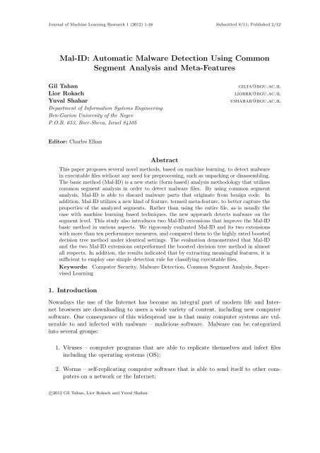
Journal of Machine Learning Research 1 (2012) 1-48 Submitted 8/11; Published 2/12 

Mal-ID: Automatic Malware Detection Using Common 

Segment Analysis and Meta-Features 

Gil Tahan 

Lior Rokach 

Yuval Shahar 

Department of Information Systems Engineering 

Ben-Gurion University of the Negev 

P.O.B. 653, Beer-Sheva, Israel 84105 

gilta@bgu.ac.il 

liorrk@bgu.ac.il 

yshahar@bgu.ac.il 

Editor: Charles Elkan 

Abstract 

This paper proposes several novel methods, based on machine learning, to detect malware 

in executable files without any need for preprocessing, such as unpacking or disassembling. 

The basic method (Mal-ID) is a new static (form-based) analysis methodology that utilizes 

common segment analysis in order to detect malware files. By using common segment 

analysis, Mal-ID is able to discard malware parts that originate from benign code. In 

addition, Mal-ID utilizes a new kind of feature, termed meta-feature, to better capture the 

properties of the analyzed segments. Rather than using the entire file, as is usually the 

case with machine learning based techniques, the new approach detects malware on the 

segment level. This study also introduces two Mal-ID extensions that improve the Mal-ID 

basic method in various aspects. We rigorously evaluated Mal-ID and its two extensions 

with more than ten performance measures, and compared them to the highly rated boosted 

decision tree method under identical settings. The evaluation demonstrated that Mal-ID 

and the two Mal-ID extensions outperformed the boosted decision tree method in almost 

all respects. In addition, the results indicated that by extracting meaningful features, it is 

sufficient to employ one simple detection rule for classifying executable files. 

Keywords: Computer Security, Malware Detection, Common Segment Analysis, Supervised 

Learning 

1. Introduction 

Nowadays the use of the Internet has become an integral part of modern life and Internet 

browsers are downloading to users a wide variety of content, including new computer 

software. One consequence of this widespread use is that many computer systems are vulnerable 

to and infected with malware – malicious software. Malware can be categorized 

into several groups: 

1. Viruses – computer programs that are able to replicate themselves and infect files 

including the operating systems (OS); 

2. Worms – self-replicating computer software that is able to send itself to other computers 

on a network or the Internet; 

c⃝2012 Gil Tahan, Lior Rokach and Yuval Shahar.

Tahan, Rokach and Shahar 

3. Trojans – a software that appears to perform the desired functionally but is actually 

implementing other hidden operations such as facilitating unauthorized access to a 

computer system; 

4. Spyware – a software installed on a computer system without the user’s knowledge to 

collect information about the user. 

The rate of malware attacks and infections is not yet leveling. In fact, according to 

O’Farrell (2011) and Symantec Global Internet Security Threat Report Trends for 2010 

(Symantec, 2010), attacks against Web browsers and malicious code variants installed by 

means of these attacks have increased. 

There are many ways to mitigate malware infection and spread. Tools such as anti-virus 

and anti-spyware are able to identify and block or identify malware based on its behavior 

(Franc and Sonnenburg, 2009) or static features (see Table 1 below). A static feature may 

be a rule or a signature that uniquely identifies a malware or malware group. While the 

tools mitigating malware may vary, at their core there must be some classification method 

to distinguish malware files from benign files. 

Warrender et al. (1999) laid the groundwork for using machine learning for intrusions 

detection. In particular, machine learning methods have been used to analyze binary executables. 

For example, Wartell el al. (2011) introduce a machine learning-based disassembly 

algorithm that segments binaries into subsequences of bytes and then classifies each subsequence 

as code or data. In this paper, the term segment refers to a sequence of bytes 

of certain size that was extracted from an executable file. While it sequentially scans an 

executable, it sets a breaking point at each potential code-to-code and code-to-data/datato-code 

transition. In addition, in recent years many researchers have been using machine 

learning (ML) techniques to produce a binary classifier that is able to distinguish malware 

from benign files. 

The techniques use three distinct stages: 

1. Feature Extraction for file representation – The result of the feature extraction phase 

is a vector containing the features extracted. An executable content is reduced or 

transformed into a more manageable form such as: 

(a) Strings – a file is scanned sequentially and all plain-text data is selected. 

(b) Portable Executable File Format Fields – information embedded in Win32 and 

Win64-bit executables. The information is necessary for the Windows OS loader 

and application itself. Features extracted from PE executables may include all 

or part of the following pieces of information: attribute certificate – similar to 

checksum but more difficult to forge; date/time stamp; file pointer - a position 

within the file as stored on disk; linker information; CPU type; Portable 

Executable (PE) logical structure (including section alignment, code size, debug 

flags); characteristics - flags that indicate attributes of the image file; DLL import 

section – list of DLLs and functions the executable uses; export section - which 

functions can be imported by other applications; resource directory –indexed by 

a multiple-level binary-sorted tree structure (resources may include all kinds of 

2

Automatic Malware Detection 

information. e.g., strings for dialogs, images, dialog structures; version information, 

build information, original filename, etc.); relocation table; and many other 

features. 

(c) n-gram – segments of consecutive bytes from different locations within the executables 

of length n. Each n-gram extracted is considered a feature (Rokach 

et al., 2008). 

(d) Opcode n-gram – Opcode is a CPU specific operational code that performs specific 

machine instruction. Opcode n-gram refers to the concatenation of Opcodes 

into segments. 

2. Feature Selection (or feature reduction) – During this phase the vector created in 

phase 1 is evaluated and redundant and irrelevant features are discarded. Feature selection 

has many benefits including: improving the performance of learning modules 

by reducing the number of computations and as a result the learning speed; enhancing 

generalization capability; improving the interpretability of a model, etc. Feature 

selection can be done using a wrapper approach or a correlation-based filter approach 

(Mitchell, 1997). Typically, the filter approach is faster than the wrapper approach 

and is used when many features exist. The filter approach uses a measure to quantify 

the correlation of each feature, or a combination of features, to a class. The overall 

expected contribution to the classification is calculated and selection is done according 

to the highest value. The feature selection measure can be calculated using many 

techniques, such as gain ratio (GR); information-gain (IG); Fisher score ranking technique 

(Golub et al., 1999) and hierarchical feature selection (Henchiri and Japkowicz, 

2006). 

3. The last phase is creating a classifier using the reduced features vector created in phase 

2 and a classification technique. Among the many classification techniques, most of 

which have been implemented in the Weka platform (Witten and Frank, 2005), the 

following have been used in the context of benign/malware files classification: artificial 

neural networks (ANNs) (Bishop, 1995) , decision tree (DT) learners (Quinlan, 

1993), nave-Bayes (NB) classifiers (John and Langley, 1995), Bayesian networks (BN) 

(Pearl, 1987), support vector machines (SVMs) (Joachims, 1999), k-nearest neighbor 

(KNN) (Aha et al., 1991), voting feature intervals (VFI) (Demiröz and Güvenir, 1997), 

OneR classifier (Holte, 1993), Adaboost (Freund and Schapire, 1999), random forest 

(Breiman, 2001), and other ensemble methods (Menahem et al., 2009; Rokach, 2010). 

To test the effectiveness of ML techniques, in malware detection, the researchers listed 

in Table 1 conducted experiments combining various feature extraction methods along with 

several feature selection and classification algorithms. 

Ye et al. (2009) suggested using a mixture of features in the malware-detection process. 

The features are called Interpretable Strings as they include both programs’ strings and 

strings representing the API execution calls used. The assumption is that the strings capture 

important semantics and can reflect an attacker’s intent and goal. The detection process 

starts with a feature parser that extract the API function calls and looks for a sequence of 

consecutive bytes that forms the strings used. Strings must be of the same encoding and 

3


character set. The feature-parser uses a corpus of natural language to filter and remove 

non-interpretable strings. Next, the strings are ranked using the Max-Relevance algorithm. 

Finally, a classification model is constructed from SVM ensemble with bagging. 

Ye et al. (2010) presented a variation of the method, presented above, that utilizes 

Hierarchical Associative Classifier (HAC) to detect malware from a large imbalanced list 

of applications. The malware in the imbalanced list were the minority class. The HAC 

methodology also uses API calls as features. Again, the associative classifiers were chosen 

due to their interpretability and their capability to discover interesting relationships among 

API calls. The HAC uses two stages: to achieve high recall, in the first stage, high precision 

rules for benign programs (majority class) and low precision rules for minority class are 

used, then, in the second stage, the malware files are ranked and precision optimization is 

performed. 

Instead of relying on unpacking methods that may fail, Dai et al. (2009) proposed a 

malware-detection system, based on a virtual machine, to reveal and capture the needed features. 

The system constructs classification models using common data mining approaches. 

First, both malware and benign programs are executed inside the virtual machine and the 

instruction sequences are collected during runtime. Second, the instruction sequence patterns 

are abstracted. Each sequence is treated as a feature. Next, a feature selection process 

in performed. In the last stage a classification model is built. In the evaluation the SVM 

model performed slightly better then the C4.5 model. 

Yu et al. (2011) presented a simple method to detect malware variants. First, a histogram 

is created by iterating over the suspected file binary code. An additional histogram 

is created for the base sample (the known malware). Then, measures are calculated to 

estimate the similarity between the two histograms. Yu et al. (2011) showed that when the 

similarity is high, there is a high probability that the suspected file is a malware variant. 

The experiments definitely proved that is possible to use ML techniques for malware 

detection. Short n-gram were most commonly used as features and yielded the best results. 

However, the researchers listed did not use the same file sets and test formats and therefore 

it is very difficult or impossible to compare the results and to determine what the best 

method under various conditions is. Table 2 presents predictive performance results from 

various researches. 

When we examined the techniques, several insights emerged: 

1. All applications (i.e. software files tested in the studies) that were developed using 

a higher level development platforms (such as Microsoft Visual Studio, Delphi, Microsoft.Net) 

contain common code and resources that originate from common code 

and resource libraries. Since most malware are also made of the same common building 

blocks, we believe it would be reasonable to discard the parts of a malware that 

are common to all kinds of software, leaving only the parts that are unique to the 

malware. Doing so should increase the difference between malware files and benign 

files and therefore should result in a lower misclassification rate. 

2. Long n-gram create huge computational loads due to the number of features. This 

is known as the curse of dimensionality (Bellman et al., 1966). All surveyed n-gram 

experiments were conducted with n-gram length of up to 8 bytes (in most cases 3-byte 

n-gram) despite the fact that short n-gram cannot be unique by themselves. In many 

4


Study 

Schultz et al. 

(2001) 

Kolter and 

Maloof (2004) 

Abou-Assaleh 

et al. (2004) 

Kolter and 

Maloof (2006) 

Feature 

Selection 

Classifiers 

NA RIPPER, Nave Bayes, 

and Multi-Nave Bayes 

n-gram NA TFIDF, Nave Bayes, 

SVM, Decision Trees, 

Boosted Decision Trees, 

Boosted Nave Bayes, and 

Boosted SVM 

n-gram NA K-Nearest Neighbors 

n-gram 

Feature 

Representation 

PE, Strings, 

n-gram 

Information- 

Gain 

K-Nearest Neighbors, 

Nave Bayes, SVM, Decision 

Trees, Boosted 

Decision Trees, Boosted 

Nave Bayes, and Boosted 

SVM. 

Decision Trees, Nave 

Bayes, and SVM 

Henchiri and n-gram Hierarchical 

Japkowicz 

(2006) 

feature selection 

Zhang et al. n-gram Information- Probabilistic Neural Network 

(2007) 

Gain 

Elovici et al. PE and n- Fisher Bayesian Networks, Artificial 

(2007) gram Score 

Neural Networks, 

and Decision Trees 

Ye et al. (2008) PE Max- Classification Based on 

Relevance Association (CBA) 

Dai et al. instruction Contrast SVM 

(2009) sequence measure 

Ye et al. (2009) PE (API) Max- SVM ensemble with bagging 

Relevance 

Ye et al. (2010) PE (API) Max- Hierarchical Associative 

Relevance Classifier (HAC) 

Yu et al. (2011) histogram NA Nearest Neighbors 

Table 1: Recent research in static analysis malware detection in chronological order. 

5


Method Study Features Feature FPR TPR Acc AUC 

selection 

Artificial Neural Elovici 5grams Fisher 0.038 0.89 0.94 0.96 

Network 

et al. 

Score top 

(2007) 

300 

Bayesian Network Elovici 5grams Fisher 0.206 0.88 0.81 0.84 

et al. 

Score top 

(2007) 

300 

Bayesian Network Elovici PE n/a 0.058 0.93 0.94 0.96 

et al. 

(2007) 

Decision Tree Elovici 5grams Fisher 0.039 0.87 0.93 0.93 

et al. 

Score top 

(2007) 

300 

Decision Tree Elovici PE n/a 0.035 0.92 0.95 0.96 

et al. 

(2007) 

Classification Ye PE Max- 0.125 0.97 0.93 —– 

Based on Association 

et al. 

Relevance 

(2008) 

Boosted Decision Kolter 4grams Gain Ratio 

—– —– —– 0.99 

Tree 

and 

Maloof 

(2006) 

Table 2: Comparison of several kinds of machine learning methods. FPR, TPR, ACC and 

AUC refers to False Positive Rate, True Positive Rate, Accuracy and the Area 

Under Receiver Operating Characteristic (ROC) Curve as defined in Section 3.2. 

6


cases 3- to 8-byte n-gram cannot represent even one line of code composed with a high 

level language. In fact, we showed in a previous paper (Tahan et al., 2010) that an 

n-gram should be at least 64 bytes long to uniquely identify a malware. As a result, 

current techniques using short n-gram rely on complex conditions and involve many 

features for detecting malware files. 

The goal of this paper is to develop and evaluate a novel methodology and supporting 

algorithms for detecting malware files by using common segment analysis. In the proposed 

methodology we initially detect and nullify, by zero patching, benign segments and therefore 

resolve the deficiency of analyzing files with segments that may not contribute or even hinder 

classification. Note that, when a segment represents at least one line of code developed using 

a high level language; it can address the second deficiency of using short features that may 

be meaningless when considered alone. Additionally, we suggest utilizing meta-features 

instead of using plain features such as n-gram. A meta-feature is a feature that captures 

the essence of plain feature in a more compact form. Using those meta-features, we are able 

to refer to relatively long sequences (64 bytes), thus avoiding the curse of dimensionality. 

2. Methods 

As explained in Section 1, our basic insight is that almost all modern computer applications 

are developed using higher level development platforms such as: Microsoft Visual Studio, 

Embarcadero Delphi, etc. There are a number of implications associated with utilizing 

these development platforms: 

1. Since application development is fast with these platforms, both legitimate developers 

and hackers tend to use them. This is certainly true for second-stage malware. 

2. Applications share the same libraries and resources that originated from the development 

platform or from third-party software companies. As a result, malware that has 

been developed with these tools generally resembles benign applications. Malware also 

tends, to a certain degree, to use the same specialized libraries to achieve a malicious 

goal (such as attachment to a different process, hide from sight with root kits, etc). 

Therefore it may be reasonable to assume that there will be resemblances in various 

types of malware due to sharing common malware library code or even similar specific 

method to perform malicious action. Of course such malware commonalities cannot 

be always guaranteed. 

3. The size of most application files that are being produced is relatively large. Since 

many modern malware files are in fact much larger than 1 MB, analysis of the newer 

applications is much more complex than previously when the applications themselves 

were smaller as well as the malware attacking them. 

The main idea presented in this paper is to use a new static analysis methodology that 

utilizes common segment analysis in order to detect files containing malware. As noted 

above, many applications and malware are developed using the development platforms that 

include large program language libraries. The result is that large portions of executable 

code originate from the program language libraries. For example, a worm malware that 

7


distributes itself via email may contain a benign code for sending emails. Consequently, since 

the email handling code is not malicious and can be found in many legitimate applications, 

it might be a good idea to identify code portions that originate from a benign source 

and disregard them when classifying an executable file. In other words, when given an 

unclassified file, the first step would be to detect the file segments that originated from 

the development platform or from a benign third party library (termed here the Common 

Function) and then disregard those segments. Finally, the remaining segments would be 

compared to determine their degree of resemblance to a collection of known malwares. If 

the resemblance measure satisfies a predetermined threshold or rule then the file can be 

classified as malware. 

To implement the suggested approach, two kinds of repositories are defined: 

1. CFL – Common Function Library. The CFL contains data structures constructed 

from benign files. 

2. TFL – Threat Function Library. The TFL contains data structures constructed 

from malware without segments identified as benign (i.e., segments that appears in 

benign files). 

Figure 1 presents the different stages required to build the needed data structures and 

to classify an application file. As can be seen in this figure, our Mal-ID methodology uses 

two distinct stages to accomplish the malware detection task: setup and detection. The 

setup stage builds the CFL. The detection phase classifies a previously unseen application 

as either malware or benign. Each stage and each sub-stage is explained in detail in the 

following subsections. The Mal-ID pseudo code is presented in Figure 2. 

2.1 The setup phase 

The setup phase involves collecting two kinds of files: benign and malware files. The benign 

files can be gathered, for example, from installed programs, such as programs located under 

Windows XP program files folders. The malware files can, for example, be downloaded from 

trusted dedicated Internet sites, or by collaborating with an anti-virus company. In this 

study the malware collection was obtained from trusted sources. In particular, Ben-Gurion 

University Computational Center provided us malware that were detected by them over 

time. Each and every file from the collection is first broken into 3-grams (three consecutive 

bytes) and then an appropriate repository is constructed from the 3-grams. The CFL 

repository is constructed from benign files and the TFL repository is constructed from 

malware files. These repositories are later used to derive the meta-features – as described 

in Section 2.2. 

Note that in the proposed algorithm, we are calculating the distribution of 3-grams 

within each file and across files, to make sure that a 3-gram belongs to the examined segment 

and thus associate the segment to either benign (CFL) or malware (TFL). Moreover, 3- 

grams that seem to appear approximately within the same offset in all malware can be used 

to characterize the malware. Before calculating the 3-grams, the training files are randomly 

divided into 64 groups. 

The CFL and TFL repositories share the same data structure: 

8


Setup phase: 

Build Common Function Library (CFL) 

Build Threats Function Library (TFL) 

Malware Detection Phase: 

Break the file into segments. 

Calculate segment entropy 

Extract features (3-grams) for 

each segment. 

For each file segment: 

Aggregate the features using the 

CFL to creates indices 

For each file segment: 

Aggregate the features using the 

TFL to creates indices 

Filter segments using the 

computed indices 

Second level index aggregation 

Classify the file 

Figure 1: The Mal-ID method for detecting new malware applications. 

Figure 1: The Mal-ID method for detecting new malware applications. 

9 

12


1. 3-gram-files-association: 2 24 entries, each of 64 bits. A bit value of 1 in a cell (i, j) 

indicates the appearance of a specific 3-gram i in the j th group of files. The 64-bit entry 

size was selected since a previous study showed that this size is the most cost effective 

in terms of detection performance vs. storage complexity (Tahan et al., 2010). Other 

implementations may use larger entries. 

1. 3-gram-relative-position-within-file: 2 24 entries, each of 64 bits. A bit value of 1 in 

a cell (i, j) indicates the appearance of 3-gram i in the j th internal segment of a file 

(assuming the file is divided into 64 equal length segments). 

The CFL is constructed first and then the TFL: 

1. Each file from the malware collection is broken into segments. The Mal-ID implementation 

has used 64-byte segments. 

2. Each segment is broken into 3grams and then tested against the CFL using the algorithm 

and features described next. Segments that are not in the CFL are added to 

the TFL. 

It is important to note that the end result is the TFL, a repository made of segments 

found only in malware and not in benign files. 

2.2 The Detection phase 

The Mal-ID basic is a feature extraction process followed by a simple static decision rule. 

It operates by analyzing short segments extracted from the file examined. Each segment 

comprises a number of 3-grams depending on the length of the segment (e.g. a segment of 

length 4 bytes is comprised from two 3-grams that overlap by two bytes). Three features 

can be derived for each segment: Spread, MFG, and Entropy. The Spread and the MFG 

features are derived using the data structures prepared in the setup stage described in 

Section 2.1 above. 

The definition and motivation behind the new features are hereby provided: 

1. Spread: Recall that in the Mal-ID setup phase each file in the training set has been 

divided into 64 relative-position-areas. The Spread feature represents the spread of 

the signature’s 3-grams along the various areas for all the files in a given repository. 

The Spread feature can be calculated as follows: for each 3-gram, first retrieve the 

3-gram-relative-position-within-file bit-field, and then perform ‘And’ operations over 

all the bit-fields and count the resulting number of bits that are equal to 1. In other 

words, spread approximates the maximum number of occurrences of a segment within 

different relative locations in train sets. For example, a Spread equal to 1 means that 

the segment appears (at most) in one relative location in all the files. 

2. MFG: the maximum total number of file-groups that contain the segment. The 

MFG is calculated using the 3-gram-files-association bit-field, in the same manner 

that spread is calculated. 

10


3. Entropy: the entropy measure of the bytes within a specific segment candidate. In 

addition to the new estimators presented above, the entropy feature is also used to 

enable to identification of compressed areas (such as embedded JPEG images) and 

long repeating sequences that contain relatively little information. 

Note that the features, as described above, are in fact meta-features as they are used 

to represent features of features (features of the basic 3-grams). As explained next, using 

these meta-features, Mal-ID can refer to relatively long sequences (64 bytes), thus avoiding 

the data mining problem known as “the curse of dimensionality”, and other problems caused 

when using short n-gram as features. The advantages of using Mal-ID meta-features will 

be demonstrated in the evaluation results section and in the discussion section. 

2.3 The Mal-ID basic detection algorithm 

The input for the Mal-ID method is an unclassified executable file of any size. Once the 

setup phase has constructed the CFL and the TFL, it is possible to classify a file F as 

benign or as malware using the algorithm presented in Figure 2. 

1. Line 1. Divide file F into S segments of length L. All segments are inserted into a 

collection and any duplicated segments are removed. The end result is a collection of 

unique segments. The Mal-ID implementation uses 2000 segments that are 64-bytes 

in length. 

2. Line 3. For each segment in the collection: 

(a) Line 5. Calculate the entropy for the bytes within the segment. 

(b) Line 6. The algorithm gets two parameters EntropyLow and EntropyHigh. The 

entropy thresholds are set to disregard compressed areas (such as embedded 

JPEG images) and long repeating sequences that contain relatively little information. 

In this line we check if the entropy is smaller than EntropyLow threshold 

or entropy is larger than EntropyHigh. Is so then discard the segment and continue 

segment iteration. Preliminary evaluation has found the values of Entropy- 

Low=0.5 and EntropyHigh=0.675 maximize the number of irrelevant segments 

that can be removed. 

(c) Line 9. Extract all 3-grams using 1 byte shifts. 

(d) Line 11. Using the CFL, calculate the CFL-MFG index. 

(e) Line 12. If the CFL-MFG index is larger than zero, then discard the segment 

and continue segment iteration. The segment is disregarded since it may appear 

in benign files. 

(f) Line 14. Using the TFL, calculate the TFL-MFG index 

(g) Line 15. The algorithm gets the ThreatThreshold parameter which indicates 

the minimum occurrences a segment should appear in the TFL in order to be 

qualified as malware indicator. In this line we check if the TFL-MFG index is 

smaller or equal to the ThreatThreshold. If so then discard the segment and 

continue with segment iteration. In the Mal-ID implementation only segments 

11


that appear two times or more remain in the segment collection. Obviously a 

segment that does not appear in any malware cannot be used to indicate that 

the file is a malware. 

(h) Line 17. Using the TFL calculate the TFL-Spread index 

(i) Line 18. The algorithm gets the SR parameter which indicates the Spread Range 

required. If the TFL-Spread index equals zero or if it is larger than what we 

term SR threshold, then discard the segment and continue segment iteration. 

The purpose of these conditions is to make sure that all 3-grams are located in 

at least 1 segment in at least 1 specific relative location. If a segment is present 

in more than SR relative locations it is less likely to belong to a distinct library 

function and thus should be discarded. In our Mal-ID implementation, SR was 

set to 9. 

(j) Lines 21-25 (optional stage, aimed to reduce false malware detection). A segment 

that meets all of the above conditions is tested against the malware file groups 

that contain all 3-gram segments. As a result, only segments that actually reside 

in the malware are left in the segment collection. Preliminary evaluation showed 

that there is no significant performance gain performing this stage more than log 

(SegmentLen) * NumberOfMalwareInTraining iterations. 

3. Lines 28-30. Second level index aggregation - Count all segments that are found in 

malware and not in the CFL. 

4. Line 32. Classify – If there are at least X segments found in the malware train set 

(TFL) and not in the CFL then the file is malware; otherwise consider the file as 

benign. We have implemented Mal-Id with X set to 1. 

Please note that the features used by Mal-ID algorithm described above are in fact metafeatures 

that describe the 3-grams features. The advantages of using Mal-ID meta-features 

will be described in the following sections. 

2.3.1 Mal-ID complexity 

Proposition 1 The computational complexity of the algorithm in Figure 2 is O(SN + 

log(SL)·M ·MaxMalSize) where SN denotes the number of segments; SL denotes segment 

length; M denotes the number of malware in the training set; and MaxMalSize denotes 

the maximum length of a malware. 

Proof The computational complexity of the algorithm in Figure 2 is computed as follows: 

the GenerateSegmentCollection complexity is O(SN); the complexity of loop number 1 

(lines 3-21) is O(SN + log(SL) · M · MaxMalSize); the complexity of loop number 2 (lines 

26-29) is O(SN). Thus, the overall complexity is O(SN + log(SL) · M · MaxMalSize). 

12


1 

2 

3 

4 

5 

6 

7 

8 

9 

10 

11 

12 

13 

14 

15 

16 

17 

18 

19 

20 

21 

22 

23 

24 

25 

26 

27 

28 

29 

30 

31 

32 

SegmentColl=GenerateSegmentCollection(FileContent,SegmentsRequired,SegmentLen); 

SegmentCheck=0; 

ForEach Segment in SegmentColl do 

{ 

Entropy = Entropy(Segment.string); 

If (Entropy= EntropyHigh) then 

{SegmentColl.delete(Segment); continue; } 

Segment3Grams:=SegmentTo3Grams(Segment); 

CFL_MFG = CFL.Count_Files_With_All_3gram (Segment3Grams) 

If (CFL_MFG>0) then { SegmentColl.delete(Segment); continue; } 

TFL_MFG = TFL.Count_Files_With_All_3gram (Segment3Grams) 

If (TFL_MFG< ThreatsThreshold) then { SegmentColl.delete(Segment); continue; } 

TFL_spread = TFL.CalcSpread (Segment3Grams); 

If (TFL_spread =0) or (TFL_spread >SR) then 

{SegmentColl.delete(Segment); continue; } 

// optional stage 

SegmentCheck++; 

If (SegmentCheck>log(SegmentLen)*NumberOfMalwareInTraining) then continue; 

InMalwareFile = TFL.SearchInMalwareFiles(Segment); //search by bit-fields 

If not InMalwareFile then { SegmentColl.delete(Segment); continue; } 

} 

SegmentsInMalwareOnly = 0; 

ForEach Segment in SegmentColl do 

{ SegmentsInMalwareOnly = SegmentsInMalwareOnly +1; } 

Malware_Classfication_Result = SegmentsInMalwareOnly > ThreatSegmentThreshold; 

Figure 2: Mal-ID pseudo code. 

Figure 2: Mal-ID pseudo code. 

Mal-ID basic 

2.4 Combining Mal-ID with ML generated models 

We attempted to improve the Mal-ID basic method by using Mal-ID features with various 

classifiers, but instead of using the Mal-ID decision model described in Section 2, we let 

various ML algorithms build the model using the following procedure: 

1. We apply the common segment analysis method on the training set and obtain a 

collection of segments for both the CFL and the TFL as explained in Section 2. 

2. For each file’s segment, we calculated the CFL-MFG, TFL-MFG and the TFL-spread 

based on the CFL and TFL. The entropy measure is calculated as well. 

13 

19


3. We discretized the numeric domain of the above features using the supervised procedure 

of Fayyad and Irani (1993). Thus for each feature we found the most representative 

sub-domains (bins). 

4. For each file we count the number of segments associated with each bin. Each frequency 

count is represented twice: once as absolute numbers (number of segments) 

and then as a proportional distribution. 

5. An induction algorithm is trained over the training set to generate a classifier. 

We compare the following three machine learning induction algorithms: 

1. C4.5 - Single Decision Tree 

2. RF - Rotation Forest (Rodriguez et al., 2006) using J48 decision tree as base classifier. 

The algorithm was executed with 100 iterations and the PCA method for projecting 

the data in every iteration. 

3. NN - A multilayer perception with one hidden layer trained over 500 epochs using 

back-propagation. 

Finally, using the model is used to detect the malware among the files in the test set. 

2.5 Combining Mal-ID with ML models post processing 

We have attempted to improve the Mal-ID basic method by using the following procedure: 

1. First, the Mal-ID basic method is used to construct the CFL and TFL. This stage is 

performed only once before the file classification starts. 

2. Next, zero patch each malware in the training set as follows: Iterate over all of the file 

segments and perform common segment analysis to detect the segments that appear 

in the CFL. The benign segments (the segments that appear in the CFL) are zero 

patched in an attempt to reduce the number of n-gram that are clearly not relevant 

for detecting segments that appear only in malware. The end result is a new file with 

the same length that has zeros in the benign segments. 

3. Finally, construct a classification model using Rotation Forest using J48 decision tree 

as base classifier. The patched malware collection and the unchanged benign file 

collection are used for training. 

To classify a file we first have to zero-patch the file as explained above then use the 

classification model created earlier. 

3. Experimental Evaluation 

In order to evaluate the performance of the proposed methods for detecting malwares, a 

comparative experiment was conducted on benchmark datasets. The proposed methods 

were compared with the method presented in the research of Kolter and Maloof (2004). 

14


The research of Kolter and Maloof (2006) found that the combination of 500 4-grams with 

gain ratio feature selection and boosted decision tree provides the best performance over 

many other evaluated method variations. We will refer to our variation of Kolter and Maloof 

method as GR500BDT as it uses Gain Ratio feature selection, 500 4-grams, and Boosted 

Decision Tree classifier. The GR500BDT method was specifically selected because it was 

the best method known to us. 

The following terms will be used when referring to the various methods: 

1. GR500BDT – Our baseline method, which is described above. 

2. Mal-IDP+GR500BDT – As explained in Section 2.5, we use Mal-ID to zero patch 

common segments in the test files, and then use GR500BDT as usual. 

3. Mal-ID basic – Mal-ID basic method as explained in Section 2. 

4. Mal-IDF+ – as detailed in Section 2.4, Mal-ID features will 

be used by induction algorithm. 

(a) Mal-IDF+RF - Mal-ID features with Rotation Forest classification 

(b) Mal-IDF+C4.5 - Mal-ID features with C4.5 

(c) Mal-IDF+NN - Mal-ID features with a multilayer perception. 

Specifically, the experimental study had the following goals: 

1. To examine whether the proposed basic methods, could detect malware while keeping 

the false alarm rate as small as possible. 

2. Compare the performance of the various Mal-ID basic extensions. 

3. To analyze the effect of the common library size (benign and malware) on performance. 

The following subsections describe the experimental set-up and the results that were 

obtained. 

3.1 Experimental Process 

The main aim of this process was to estimate the generalized detection performance (i.e., 

the probability that a malware was detected correctly). The files repository was randomly 

partitioned into training and test sets. The process was repeated 10 times and we report 

the average result. The same train-test partitioning was used for all algorithms. 

For evaluating the proposed methodology 2627 benign files were gathered from programs 

installed under Windows XP program files folders, with lengths ranging from 1Kb to 24MB. 

An additional 849 malware files were gathered from the Internet with lengths ranging from 

6Kb to 4.25MB (200 executables were above 300KB). The detailed list of examined executables 

can be obtained in the following URL: http://www.ise.bgu.ac.il/faculty/liorr/List.rar. 

The malware and benign file sets were used without any decryption, decompression or any 

other preprocessing. The malware types and frequencies are presented in Figure 3. The 

evaluation computer used an Intel Q6850 CPU with 4GB of RAM. The processing time was 

measured using only 1 CPU core, although the implemented algorithm natively supported 

multiple cores. 

15


Email Worms, 209, 

25% 

Worm, 43, 5% 

P2P, 43, 5% 

Flooder, 43, 5% 

Denial Of Service 

(DoS), 53, 6% 

Email Flooder, 57, 

7% 

Virus, 232, 27% 

Trojan, 100, 12% 

Exploits, 69, 8% 

Worm P2P Flooder 

Denial Of Service (DoS) Email Flooder Exploits 

Trojan Virus Email Worms 

Figure 3: Distribution of malware types in dataset. 

Figure 3: Distribution of malware types in dataset. 

3.2 Evaluation Measures 

23 

We used the following performance measures: 

• TP = true positive 

• FP = false positive 

• TN = true negative 

• FN = false negative 

• FPR = FP / N = FP / (FP + TN) = false positive rate 

• TPR = TP / P = TP / (TP + FN) = true positive rate (also known as sensitivity) 

• PPV = TP / (TP + FP) = positive predictive value 

• NPV = TN / (TN + FN) = negative predictive value 

• ACC = (TP + TN) / (P + N) = accuracy 

• BER = 0.5(FN/P + FP/N) = balanced error rate 

• BCR = 1- BER = balanced correctness rate 

16


• AUC = area under receiver operating characteristic (ROC) curve 

Our measures, such as PPV versus NPV, as well as BER or BCR, try to address the 

important case of an unbalanced positive/negative instance case mix, which is often ignored 

in the literature. Given the low rate of malware versus benign code, accuracy might be 

a misleading measure. For example, a “Maximal Class Probability” (MPC) classifier is a 

classifier that always predicts the most frequent class. Thus, an MPC predicting “BENIGN” 

for every instance in an environment where 99% of the files are benign would, indeed, be 

99% accurate. That would also be its NPV, since there is a 99% probability that the MPC 

is right when it predicts that the file is benign. However, its PPV would be 0, or rather, 

undefined, since it never predicts a positive class; in other words, its sensitivity to positive 

examples is 0. 

Furthermore, unlike many studies in the information security literature, we use the 

cross-entropy as one of our major performance measures. The cross-entropy described by 

Caruana et al. (2004). It is also referred in the literature by the terms negative log-likelihood 

or log-loss. Let p(x i ) represents the posterior probability of the instance x i to be associated 

with the malware class according to the classifier. The average cross-entropy is defined as 

the average over all m test instances: 

Entropy = 1 m 

m∑ 

I(x i ) 

i=1 

where the cross-entropy for a certain case is defined as: 

{ 

−logP (x 

I (x i ) = 

i ) if x i is malware 

−log (1 − P (x i )) otherwise 

The use of cross-entropy as a measure of knowledge gain allows us to plot the improvement 

in a learning process, given an increasing number of examples, by noting whether there 

is a positive information gain (i.e., a reduction in the entropy after learning, compared to 

the entropy of the previous learning phase). In particular, we would expect an algorithm 

that really learns something about the classification of both the positive and negative cases 

to demonstrate a positive monotonic improvement in the cross-entropy measure. It is important 

to show this positive monotonic improvement since we would prefer an algorithm 

that generates classifiers in a stable fashion. Such an algorithm can be considered as more 

trustworthy than an algorithm whose learning curve might be chaotic. 

3.3 Results 

The following sections describe various Mal-ID evaluation results starting with the Mal- 

ID basic model followed by the results of two enhancements aimed to improve Mal-ID 

performance. 

3.3.1 Results of Mal-ID basic Model 

Table 3 presents the detection performance of the proposed method for 70% of the benign 

files and 90% of the malware files that are used for training. 

17


TPR FPR PPV NPV AccuracyAUC BCR BER 

0.909 0.006 0.944 0.99 0.986 0.951 0.952 0.048 

Table 3: Predictive Performance of Mal-ID basic. 

Kolter and Maloof (2006) conducted rigorous research to find the best combination of 

n-gram length, n-gram number, features selection and classification method. They reported 

that the combination of five hundred 4-grams, gain ratio feature selection and boosted 

decision tree (AdaBoost.M1 with J48 as a base classifier) produced excellent results where 

the AUC was over 0.99. As you recall, we reproduced the work of Kolter and Maloof (gain 

ratio, 500 4-grams with boosted decision tree; referred to as GR500BDT ) to objectively 

compare the performance of our methods and theirs under the same conditions such as 

dataset content, dataset training size, etc. A preliminary evaluation indicated that Rotation 

Forest (RF) boosting method (Rodriguez et al., 2006) performed better than AdaBoost.M1 

and many other non-boosting methods such as J48, therefore RF was selected for our 

evaluation. The results of the evaluation are presented in Table 4 below. 

Method Features Feature selection FPR TPR Acc AUC 

GR500BDT 4grams Gain Ratio 0.094 0.959 0.948 0.929 

Mal-ID Mal-ID - 0.006 0.909 0.986 0.951 

Table 4: Comparison between Mal-ID and GR500BDT. The best results are colored with 

blue and the worst results are colored in red. 

3.3.2 Results of combining Mal-ID with ML generated models 

As you recall we attempted to improve the Mal-ID basic method by using Mal-ID features 

with various classifiers. The following figures show comparison of various detection performance 

measures. Many detection performance measures were recorded and reported as 

presented in the figures below. Please note that ”TrainPercentage” refers to the percentage 

of benign datasets and ranges from 30 to 70 percent. Malware dataset percentages range 

from 40 to 90 percent. The ratio between malware and benign was kept fixed for all cases. 

Figure 4 reports the average cross-entropy for a classifier by averaging the entropy of 

the posteriori probability that it outputs to all test instances. As expected, we see that 

the cross-entropy decreases as the training set size increases. For the largest training set, 

Mal-ID basic shows the best decrease in a posteriori cross-entropy. 

Figure 5 presents the accuracy of the Mal-ID basic model as well that of the Mal- 

IDF+NN and Mal-IDF+RF models. As expected, the accuracy increases almost linearly 

as the training set size increases. For small training set sizes, Mal-IDF+RF outperforms 

the other methods. However, for the largest training set, the Mal-ID basic model eventually 

achieves the best results. 

Figure 6 presents the TPR of all methods. Mal-IDF+C4.5 demonstrates the lowest 

TPR. The Mal-IDF+NN and Mal-IDF+RF models perform the best. The Mal-ID basic 

model benefits the most from increasing the training set size. In small training sets, 

the difference between the Mal-ID basic model and either Mal-IDF+NN or Mal-IDF+RF 

18


are statistically significant. However, for larger training sets the differences are no longer 

significant. 

Figure 4: Comparing the a posteriori cross-entropy of various detection modules as a function 

of training set percentage increase. 

Figure 7 presents the FPR of all methods. The Mal-ID basic model demonstrates the 

best performance. Mal-IDF+C4.5, on the other hand, demonstrates the lowest FPR. The 

performance of Mal-IDF+NN does not improve as the training set increases. The Mal- 

ID basic model significantly outperforms Mal-IDF+C4.5 and Mal-IDF+NN. Additionally, 

a paired t-test indicates the Mal-ID basic’s FPR is significantly lower than the FPR of 

Mal-IDF+RF with p < 0.0001. 

Figure 8 presents the area under the ROC curve for the Mal-ID basic model, Mal- 

IDF+NN and Mal-IDF+RF. All models improve as the training set increases. The Mal-ID 

basic model shows the lowest AUC but also benefits the most from increasing the training 

set size. The lower AUC of the Mal-ID basic model can be explained by the fact that 

contrary to the other models, the Mal-ID basic model is a discrete classifier. Discrete 

classifiers produce only a single point in ROC space (Fawcett, 2004) and therefore their 

calculated AUC appears lower. 

When we examined the balanced error rate (BER) for Mal-ID basic, Mal-IDF+NN and 

Mal-IDF+RF Models, we noticed that the BER measure decreases for all models as the 

training set increases. Mal-ID basic demonstrated a significant and sharp decline in the 

BER as the training set increases. In almost all cases, the Mal-IDF+RF achieved the 

lowest BER. With the largest training set there is no significant difference between the 

Mal-ID basic model and the Mal-IDF+RF model. 

19 

28 

Mal-ID basic



Figure 5: Comparing the accuracy performance of the Mal-ID basic model with the machine 

learning methods on various training set size percentages. 

28 

When we compared the NPV of the Mal-ID basic model with the NPV of the Mal- 

IDF+NN and Mal-IDF+RF, we noticed, as expected, that the NPV increases almost linearly 

as the training set size increases. For small training set sizes, Mal-IDF+RF and 

Mal-IDF+NN outperform the other methods. Eventually, however, there is no statistically 

significant difference for the largest training set. 

When we compared the PPV of the Mal-ID basic model with the PPV of the Mal- 

IDF+NN, Mal-IDF+C4.5 and Mal-IDF+RF, we found out that Mal-ID basic has the best 

PPV for all training set sizes. The Mal-IDF+RF performed better than the Mal-IDF+NN 

and the Mal-IDF+NN performed better than Mal-IDF+C4.5. 

To sum up, in many cases Mal-ID basic outperforms the methods that use Mal-ID 

features combined with a ML classifier and we conclude that a simple decision rule is 

sufficient. 

3.3.3 Combining Mal-ID with ML models post processing 

As you recall, we have attempted to improve the Mal-ID basic method by using the method 

to zero-patch the benign common library parts. To measure and compare the effect of 

the Mal-ID patching prior to classifying, we preformed an evaluation using four methods: 

GR500BDT, Mal-IDF+GR500BDT, Mal-ID basic, and Mal-IDF+RF. 

20



Figure 6: Comparing the true positive rate of the Mal-ID basic model with the machine 



Mal-IDF+C4.5 

Mal-IDF+NN 

Mal-IDF+C4.5 Mal-IDF+NN 


IDF+NN Mal-IDF+RF 

ID basic 


Mal-ID 

The 

Figure 9 compares the accuracy performance using various training set sizes. 

results 

basic 

show that with Mal-IDP+GR500BDT we were able to improve performance but 

only on relatively small training sets. However, compared to the known GR500BDT, Mal- 

IDP+GR500BDT show significant and consistent improvements in accuracy by about 2%. 

All Mal-ID 

IDF+RF 

variations were able to outperform GR500BDT regardless of training set size. 

It should be noted that on the one hand we should have expected to an improvement in 

the predictive performance when the training set size increases. On the other hand because 

we also increase the imbalance ratio between benign and malware therefore we should have 

expected to a decrease in the predictive performance. Eventually we observe that accuracy 

of GR500BDT remains almost constant. 

Mal- 



Figure 10 compares FPR performance under various training set sizes. The results 

indicate that there is slight but constant improvement in terms of FPR when first performing 


a patch with Mal-ID (Mal-IDP+GR500BDT ) instead of using n-gram without patching 

(GR500BDT ). The performance of all n-gram-based 


methods decreases 

discrete 

sharply when the 

training set consists of more than 50% benign files. The graph shows that in terms of FPR, 

the Mal-ID basic method always performs slightly better than the Mal-IDF+RF method 

and both methods perform significantly better than n-gram based methods. In other words, 

the graph shows that in terms of FPR, there is a significant difference between methods 

that utilize n-gram features and those that utilize the Mal-ID meta-features. 

21 

29



Figure 7: Comparing the false positive rate of the Mal-ID basic model with the machine 


Table 5 summarizes the detection performance results for the various Mal-ID methods 

and the GR500BDT baseline and can help in choosing the best method when considering 

detection performance only. Other important considerations will be discussed below. The 

results demonstrate that Mal-IDP+GR500BDT always outperforms GR500BDT baseline 

and Mal-IDP+GR500BDT should be used when the highest TPR is desired and a high FPR 

is acceptable. However Mal-ID basic and Mal-IDF+RF seems to be the best choice for more 

balanced performance with extremely low FPR and for achieving the highest accuracy. 

Method Feature selection FPR TPR Acc AUC 

GR500BDT (un-patched + Gain Ratio 0.094 0.959 0.948 0.929 

RF) 

Mal-IDP+GR500BDT Gain Ratio 0.093 0.977 0.963 0.946 

(patched + RF) 

Mal-ID basic Mal-ID 0.006 0.909 0.986 0.951 

Mal-IDF+RF (Mal-ID features 

None 0.006 0.916 0.985 0.995 

+ 

RF) 

Table 5: A comparison of various Mal-ID methods and RF when using maximum training 

size. The best results are colored with blue. 


22 

30




Figure 8: Comparing the AUC of the Mal-ID basic model with the machine learning methods 

on various training set size percentages. 

30 

Table 6 presents the training time (in seconds) and detection time (in ms) of all examined 

methods. The evaluation computer used an Intel Q6850 CPU with 4GB of RAM. All times 

were measured using only 1 CPU core. The training time of Mal-ID based methods does not 

include building the CFL and TFL which took around 30 seconds. As expected the training 

time increases with the training size. In addition, GR500BDT training time does not include 

the n-gram feature extraction and selection (which took more than ten minutes). The Mal- 

ID basic and Mal-IDF+C4.5 methods demonstrated the best training time performance 

with less than one second. The detection time seems almost constant regardless of training 

set size. The only exception is Mal-IDF+RF in which detection time increases almost 

linearly as the training set increases. Note that the size of the trees (number of nodes) 

which constitute the rotation forest usually increases with the training set. This can be 

explained by the fact that the number of leaves in the tree is bounded by the training set 

size. Larger trees require a longer traversal time and features calculation. Recall that in 

rotation forest, the features used in the various nodes are linear combination of the original 

features. 

Table 7 reports the mean TPR of Mal-ID basic for small malwares (size350K) using the largest training set. Note that the FPR is kept as 

reported in Table 5 (i.e. FPR=0.006). The results show that the TPR for both small 

23

500BDT 


Accuracy 

100.0 

99.5 

99.0 

98.5 

98.0 

97.5 

97.0 

96.5 

96.0 

95.5 

95.0 

94.5 

94.0 

93.5 

DataShort*Method; LS Means 

Current effect: F(12, 175)=7.5601, p=.00000 

Effective hypothesis decomposition 

Vertical bars denote 0.95 confidence intervals 

30 40 50 60 70 

Percentage 

Ngram 

Ngram-patched 

Expert 

RF 

Figure 9: Comparing the accuracy of various Mal-ID-based methods and the n-gram 

method on various training set size percentages. 

Mal-IDF+RF 


Mal-IDP+GR500BDT 

Train Percentage 

Method 30 40 50 60 70 

Training MalID-Basic 

GR500BDT 

0.05 0.08 0.11 0.15 0.21 

Time Mal-IDF+RF 17.19 26.00 36.35 45.78 83.50 

(in sec) Mal-IDF+C4.5 0.12 0.17 0.22 0.33 0.43 

Mal-IDF+NN 24.33 32.16 40.33 48.37 56.93 

GR500BDT 21.74 34.91 59.86 64.88 75.19 

Mal-IDP+GR500BDT 20.93 31.42 42.96 55.65 63.43 

Detection MalID-Basic 27.86 27.86 27.86 27.86 27.86 

Time Mal-IDF+RF 49.17 54.69 63.66 73.95 95.82 

per file Mal-IDF+C4.5 27.86 27.86 27.86 27.86 27.86 

(in ms) Mal-IDF+NN 27.92 27.92 27.90 27.89 27.88 

GR500BDT 29.63 29.83 29.83 29.85 29.83 

Mal-IDP+GR500BDT 29.01 29.01 29.02 28.98 28.97 

Table 6: Training and32 

Detection Time. 

and large group is very similar indicating that MAL ID is not affected by the size of the 

examined malware. 

24


0.12 

DataShort*Method; LS Means 

Current effect: F(12, 175)=3.7074, p=.00005 

Effective hypothesis decomposition 

Vertical bars denote 0.95 confidence intervals 

0.10 

False Positive Rate 

0.08 

0.06 

0.04 

0.02 

0.00 

30 40 50 60 70 

DataShort 

Ngram 

Ngram-patched 

Expert 

RF 

Figure 10: Comparing the FPR of various Mal-ID-based methods and the n-gram method 

on various training set size percentages. 

GR500BDT 

Malware Size TPR Number of Mean Size 

Malwares 

Small 0.909 675 96K 

Large 0.908 174 554K 

Mal-IDP+GR500BDT 

Mal-IDP+GR500BDT Mal-ID basic Mal-IDF+RF 

GR500BDT 

Table 7: A comparison of TPR (True Positive Rate) Mal-ID basic for small and large malwares 

when using maximum training size. 

In order to estimate the effect of obfuscation on detection rate, we have divided the tested 

malware into two groups –obfuscated and non-obfuscated. Because we were not informed 

which executable was obfuscated, we have used the following method. We compressed 

the executables using Zip and sorted them according to the compression ratio. We used 

a threshold GR500BDT of 50% compression (un-patched + ratio RF) to decide Gain which Ratioexecutable 0.094 is0.959 probably 0.948 obfuscated. 0.929 

The selection Mal-IDP+GR500BDT of this threshold (patched was based + RF) on experiments Gain Ratio of 0.093 compressing 0.977 non- 0.963obfuscated 

0.946 

executables. 


According 

basic 

to this threshold, about 


37.5% of the malware 

0.909 

are considered 

0.951 

to 

be obfuscated. 

Mal-IDF+RF 

Table 

(Mal-ID 

8 reports 

features 

the mean 

+ RF) 

TPR 

None 

of Mal-ID basic for 

0.916 

obfuscated 

0.985 

and nonobfuscated 

groups using the largest training set. Note that the FPR is kept as reported in 

Table 5 (i.e. FPR=0.006). The results show that the TPR for both obfuscated and nonobfuscated 

group is very similar with slight advantage to detecting obfuscated malwares. 

25 

33


There might be several reasons that can explain why the TPR of obfuscated binaries 

appears to be higher than the TPR of non-obfuscated binaries. One reason can be that many 

obfuscated malwares are generated by automated tools that have distinctive properties. 

For example, malware developers are sharing tools for facilitating the generation of new 

malwares. For example, in the web site http://vx.netlux.org/, one can find many tools 

(such as Falckon Encrypter that is used for obfuscation) that can be used by the malware 

developers but are not used by benign software developers. All malware that utilize the 

Falckon Encrypter, share the same decryption segment. 

Malware type 

TPR Mean Compression 

Ratio 

Obfuscated 0.932 41% 

Non-obfuscated 0.893 62% 

Table 8: A comparison of TPR (True Positive Rate) Mal-ID basic for obfuscated and nonobfuscated 

malware when using maximum training size. 

4. Discussion 

This paper proposes a new approach for automatically detecting executable malwares of all 

kinds and sizes. The results show that using the Mal-ID basic and other Mal-ID variants 

are useful in detecting malware. As can be seen from Table 3, the Mal-ID basic method 

performs very well in respect to all measures. Not only is the accuracy very high (0.986), 

but the FPR is remarkably low (0.006). In addition, the low Mal-ID BER indicates that 

the errors are almost uniformly distributed among the malicious and benign files. 

As explained in Section 3.3.1, we choose to implement GR500BDT as a baseline for 

comparing the performance of the Mal-ID basic method. GR500BDT is very similar to 

the method proposed by Kolter and Maloof (2006). The evaluation shows that GR500BDT 

performed well, but was unable to achieve the AUC of 0.995 that Kolter and Maloof reported. 

This was probably due to differences in dataset content, training size, the benign 

and malware ratio and possibly other factors. As can be seen from Table 4, under identical 

conditions the Mal-ID methodology was able to outperform GR500BDT in terms of FPR, 

accuracy and AUC. The FPR of GR500BDT method came to almost 10%; Mal-ID FPR 

was more than 15 times lower. 

Once it was established that the Mal-ID basic method performs well (in fact better than 

the best baseline method) we wanted to examine Mal-ID behavior with different train sizes 

to test if Mal-ID basic performs in a stable and “trustworthy” manner. In addition, it was 

interesting to determine if combining Mal-ID basic with ML-generated models, as explained 

in Section 3.3.2, would yield a better performing malware detection method. 

The results presented in Figure 4 to Figure 8 show that combining Mal-ID with MLbased 

models enabled us to improve many aspects of the Mal-ID basic method when training 

sets are not maximal. However, as training set size increases, the benefit of combining Mal- 

ID basic with ML-based models diminishes. At maximal training set size, the Mal-ID 

basic method almost always demonstrates the best performance or a performance that is 

26


statistically equal to the combined methods. It is also important to note that, contrary 

to the other methods, all measures that we implemented indicated that the Mal-ID basic 

method benefited the most from training set increase and always performed in an expected 

manner. Thus, it may be considered more stable and “trustworthy” than the other methods. 

It is interesting to note that while the performance of non-n-gram methods (Mal-ID 

basic and Mal-IDF+RF ) continues to improve as more training data become available, 

the n-gram based methods show a sharp decrease in performance in terms of FPR (see 

Figure 10). This can be explained by the fact that n-gram methods induce relatively simple 

patterns that can be learned with comparatively small training sets (30%). The potential 

benefit of additional training data is nullified by the undesirable increase in the probability 

that relevant n-gram will be mistakenly considered as non-contributing features. In fact, it 

is well known that decision trees increase their chances of overfitting when they have more 

nodes. But in order to have more nodes, they need a larger training set. Thus a larger 

dataset might increase the chance of overfitting especially in cases were there are many 

irrelevant and noisy features. 

The comparison of our two additional methods, Mal-IDF+RF and Mal-IDP+GR500BDT, 

with a GR500BDT baseline is very important in proving the validity of Mal-ID itself and 

explaining its excellent performance: 

1. (a) Under identical conditions, boosted decision tree, operating on Mal-ID basic 

meta-features (Mal-IDF+RF ), outperformed boosted decision tree operating on 

n-gram (GR500BDT ). The comparison suggests that Mal-ID meta-features are 

useful in contributing to malware detection and probably more meaningful than 

simple n-gram in capturing a file’s essence. 

(b) Under identical conditions, boosted decision tree operating on Mal-ID basic 

patched files (Mal-IDP+GR500BDT ) outperformed boosted decision tree operating 

on non-patched files (GR500BDT ). The comparison suggests that the 

novel Mal-ID common segment analysis approach is better than the common 

approach that treats files as black boxes or which interprets files PE header only. 

Since Mal-ID basic and Mal-IDF+RF methods benefit from both more meaningful features 

and common segment analysis, they are able to achieve a better overall performance 

than state-of-the-art GR500BDT. 

Considering detection performance only when choosing a malware detection method 

may not be enough; it is important to consider other aspects as well. 

4.1 Model interpretability 

Mal-ID basic uses only one static interpretable classification model and therefore experts in 

the field can be more confident when accepting or rejecting a classification. For instance, 

once Mal-ID basic has detected a yet unknown malware, it is possible to support or reject 

the classification. The reason is that each detected segment, that passed the Mal-ID filter 

stage as explained in Section 2, can be tracked back to a specific malware or malware 

group. Moreover, the specific offset location were the segments appear can be examined to 

determine the precise nature of the threat, if any exists. Disassembly or reverse engineering 

of the whole malware is no longer required. Even without examining the segment code, one 

27


can make an educated guess about the nature of the threat by examining the list of known 

malwares that the segment appears in. The other methods do not provide such benefits. 

4.2 Incremental 

As more malwares are discovered, it is important to update the models from time to time. 

With Mal-ID basic it is particularly easy. Since the model is static, no reconstruction is 

necessary; all that is required is to just to add or subtract files from the TFL. The CFL can 

be updated in a similar manner. 

4.3 Anytime Detection 

Recall that both Mal-ID basic and Mal-IDF+RF operates on segments. Because Mal-ID 

basic and Mal-IDF+RF use relatively large segments and the model is not comprised of 

combined features from the whole file, it is possible to stop detection at anytime during 

file scan and determine if the scanned part is malicious. n-gram-based methods are not 

designed to diagnose part of file but rather whole files only. 

4.4 Default signature for real-time malware detection hardware 

The end result of applying Mal-ID basic method is a file segment or segments that appear 

in malware files only and thus may be used as a signature for anti-virus tools. The detected 

malware segments can be used, as described by Filiol (2006), to generate signatures resistant 

against black-box analysis. Moreover, because Mal-ID basic produces a simple signature 

and has anytime detection traits, the signature can be used with commercially available 

real-time intrusion prevention systems (IPS). IPSs require the anytime detection trait to 

act as real-time malware filtering devices and thus promote and provide users with default 

protection. Having both malware detection and signature generation could help shorten 

the window of vulnerability. Tahan et al. (2010) have presented a methodology with complete 

implementation for automatic signature generation, utilizing similar and compatible 

techniques, which archived excellent results in the evaluation. Thus, the method presented 

by Tahan et al. (2010) can be easily adopted to produce signature upon detection for the 

solution presented in this paper. 

4.5 Large files scalability 

Nowadays it’s quite common to embed large resources such as JPEG pictures and small 

animations into executables. This inflation is also true for malware. It is estimated 1 that 

the mean malware size has increased from 150K (in 2005) to 350K (in 2010). As files become 

larger, the effectiveness of classification with small n-gram should decrease due to the 

increase in file entropy. In other words, the more n-gram with equal appearance probability, 

the greater the misclassification probability becomes. Since Mal-ID basic and Mal-IDF+RF 

use relatively large segments (64 bytes) and in addition filter-out high entropy parts, they 

should be less susceptible to misclassification caused by large files or files with high entropy 

traits. Figure 10 shows that the Mal-ID methods that operate on large segments (of 64 

1. http : //nakedsecurity.sophos.com/2010/07/27/large − piece − malware/ 

28


bytes) has less FPR misclassification then the method that operated on small n-gram (of 4 

bytes). We further examined this hypothesis in Table 7. 

4.6 Analysis of Mal-ID performance on Obfuscated Malware 

Based on the results presented so far, we hypothesize that the proposed Mal-ID method 

performs well in a mixed environment where both obfuscated (including compressed or 

encrypted) and plain executable files exist. In this sense, we referred to malware as they 

are found “in the Wild”. 

The results of Table 8 agree with the previously-made observation that ML techniques 

can classify malware that are obfuscated (compressed or encrypted or both). For example, 

Kolter and Maloof (2006) have noted that ML can detect obfuscated malware. In this paper, 

we have independently reconfirmed the validity of the above observation using our method. 

In this experiment, we succeeded to keep FPR relatively low (FPR=0.006), however it 

should be noted that this value was obtained when our corpus contained 2,627 benign files 

and 849 malware files (i.e. a benign to malware ratio of 3:1). In reality this ratio can be 

much higher and therefore one should expect to obtain elevated FPR values. 

There seem to be previously suggested explanations to this phenomenon. According to 

Kolter and Maloof (2006), the success in detecting obfuscated malware relies on learning 

certain forms of obfuscation such as run-time decompression. Kolter and Maloof (2006) 

conclude that “. . . this does not seem problematic as long as those forms are correlated with 

malicious executables”. 

Additional explanations can be suggested to the ability to identify obfuscated malware. 

Studies such as that presented by Newsome and Song (2005), or by Newsome et al. (2005) 

noticed that in many cases malware requires fixed sequences to be used in the body of the 

malware (which must exist before self-decryption or self-decompression) in order to exploit 

a specific vulnerability and self-propagate. Such fixed sequences can be used for detection. 

This might explain the success in detecting obfuscated malware. 

Because the performance of MAL ID is achieved with no disassembly, Op-Code analysis, 

executable header analysis, unpacking nor any other preprocessing, we hypothesize that the 

method should be scalable to other Operating Systems and hardware types. Still one 

can think on cases where preprocessing will be required. Theoretically an attacker can 

specifically design a malware that will make it hard for MAL ID to detect it. In particular, 

if a malware is designed such that the entropy measure will be high for all segments, it 

will be undiscovered by the Mal-ID basic method. In this case Mal-ID can be extended 

by incorporating an unpacker operating before it, such as those that are incorporated into 

anti-viruses tools (Kasparsky). However, similar to Kolter and Maloof (2006), we decided 

to evaluate the raw power of our methods without any use of an unpacker. 

5. Summary and Future Work 

In this paper we have described novel methods based on machine learning to detect malware 

in executable files without any need for preprocessing the executables. The basic method 

that we presented works on the segment level for detecting new malware instead of using 

the entire file as usually done in machine learning based techniques. The Mal-ID basic 

method and its derived variants were rigorously tested to evaluate their effectiveness under 

29


many conditions using a wide variety of measures. The results demonstrate the effectiveness 

of the methods. In all cases, most of the performance measures showed that the proposed 

methods significantly outperformed the baseline method GR500BDT which is known for its 

excellent performance (Kolter and Maloof, 2004, 2006). For each method we have pinpointed 

its strong points and suggested cases where it should be preferred over the others. 

We believe this study has made several contributions to malware detection research, 

including the introduction of: 

1. a new and effective method for malware detection based on common segment analysis 

and supporting algorithms. The importance of common segment analysis to the process 

of malware detection was identified and demonstrated. The results suggest the 

method can boost performance for many methods that utilize n-gram. 

2. new kinds of features - Mal-ID basic meta-features. The results suggest that the metafeatures 

are much more effective than the commonly used n-gram and probably more 

meaningful in terms of file representation. We believe that Mal-ID basic meta-features 

could inspire many kinds of additional meta-features that could prove useful. 

3. BCR, BER, PPV, NPV and entropy decrease for measuring the performance of malware 

detection methods. Using these measures, in addition to the commonly utilized 

performance measures (TPR, FPR, accuracy and AUC), is not generally practiced. 

However, these features are helpful in describing the behavior of a new method, particularly 

when it is not possible to compare results under identical settings and dataset 

imbalance. 

The results also indicate that by extracting meaningful features, it is sufficient to employ 

one simple detection rule for classifying unknown executables. 

In the future, we aim to examine the effect of systematically collecting and choosing 

the benign file set on the performance of the proposed methods. In the evaluations that 

were conducted for this study, the benign file set was collected randomly and the files 

used may have had a large degree of similarity. It is our assumption that systematically 

collecting and choosing common segments will provide a better representation of benign 

common segments and a more robust and lower FPR. A robust and low FPR will enable 

the use of more sensitive malware detection methods (or parameters that affect malware 

detection) without increasing the FPR too much. As a result, we hope to see further 

increase in the AUC measure. Finally the Mal-ID basic method was developed as a crisp 

classifier. Additional research is required for developing a method for ranking the examined 

files according to their presumed threat level. One straightforward measure is the ratio 

between the segments found in the TFL and the segments found in the CFL. In addition, it 

will be interesting to test the proposed method on live network data and on an institutional 

network and determine if it detects malware that is not detected by other means. Finally, 

future work may repeat the evaluation Mal-ID on a larger scale with thousands of malware 

samples and tens of thousands of non-malware samples. For this purpose, we might need 

to upscale software components to accommodate large dataset and suitable hardware. In 

addition, in order to use the proposed method in practice by the industry, fine tuning of 

the various parameters might be required. 

30


Additional studies might be needed to fully evaluate the performance of Mal-ID under 

various obfuscation scheme, including use of recursive unpacking. In this paper we focused 

only on “pure” Mal-ID methods and therefore we did not investigate the proper means to 

incorporate unpacker. 

Acknowledgments 

The authors gratefully thank the action editor, Prof. Charles Elkan and the anonymous 

reviewers whose constructive comments considerably strengthened this manuscript. 

References 

T. Abou-Assaleh, N. Cercone, V. Keselj, and R. Sweidan. N-gram-based detection of new 

malicious code. In Computer Software and Applications Conference, 2004. COMPSAC 

2004. Proceedings of the 28th Annual International, volume 2, pages 41–42. IEEE, 2004. 

D.W. Aha, D. Kibler, and M.K. Albert. Instance-based learning algorithms. Machine 

learning, 6(1):37–66, 1991. 

R.E. Bellman, R.E. Bellman, R.E. Bellman, and R.E. Bellman. Adaptive control processes: 

a guided tour. Princeton University Press, 1966. 

C.M. Bishop. Neural networks for pattern recognition. 1995. 

L. Breiman. Random forests. Machine learning, 45(1):5–32, 2001. 

R. Caruana, T. Joachims, and L. Backstrom. Kdd-cup 2004: results and analysis. ACM 

SIGKDD Explorations Newsletter, 6(2):95–108, 2004. 

J. Dai, R. Guha, and J. Lee. Efficient virus detection using dynamic instruction sequences. 

Journal of Computers, 4(5):405–414, 2009. 

G. Demiröz and H. Güvenir. Classification by voting feature intervals. Machine Learning: 

ECML-97, pages 85–92, 1997. 

Y. Elovici, A. Shabtai, R. Moskovitch, G. Tahan, and C. Glezer. Applying machine learning 

techniques for detection of malicious code in network traffic. KI 2007: Advances in 

Artificial Intelligence, pages 44–50, 2007. 

T. Fawcett. Roc graphs: Notes and practical considerations for researchers. ReCALL, 31 

(HPL-2003-4):1–38, 2004. 

Usama M. Fayyad and Keki B. Irani. Multi-interval discretization of continuous-valued 

attributes for classification learning. In IJCAI, pages 1022–1029, 1993. 

E. Filiol. Malware pattern scanning schemes secure against black-box analysis. Journal in 

Computer Virology, 2(1):35–50, 2006. 

31


V. Franc and S. Sonnenburg. Optimized cutting plane algorithm for large-scale risk minimization. 

The Journal of Machine Learning Research, 10:2157–2192, 2009. 

Y. Freund and R.E. Schapire. A brief introduction to boosting. In International Joint Conference 

on Artificial Intelligence, volume 16, pages 1401–1406. LAWRENCE ERLBAUM 

ASSOCIATES LTD, 1999. 

T.R. Golub, D.K. Slonim, P. Tamayo, C. Huard, M. Gaasenbeek, J.P. Mesirov, H. Coller, 

M.L. Loh, J.R. Downing, M.A. Caligiuri, et al. Molecular classification of cancer: class 

discovery and class prediction by gene expression monitoring. science, 286(5439):531, 

1999. 

O. Henchiri and N. Japkowicz. A feature selection and evaluation scheme for computer 

virus detection. In Data Mining, 2006. ICDM’06. Sixth International Conference on, 

pages 891–895. IEEE, 2006. 

R.C. Holte. Very simple classification rules perform well on most commonly used datasets. 

Machine learning, 11(1):63–90, 1993. 

Thorsten Joachims. Making large-scale svm learning practical. Advances in Kernel Methods 

Support Vector Learning, pages 169–184, 1999. 

G.H. John and P. Langley. Estimating continuous distributions in bayesian classifiers. In 

Proceedings of the eleventh conference on uncertainty in artificial intelligence, volume 1, 

pages 338–345. San Mateo, 1995. 

Jeremy Z. Kolter and Marcus A. Maloof. Learning to detect malicious executables in the 

wild. In Proceedings of the tenth ACM SIGKDD international conference on Knowledge 

discovery and data mining, KDD ’04, pages 470–478, New York, NY, USA, 2004. ACM. 

ISBN 1-58113-888-1. 

J.Z. Kolter and M.A. Maloof. Learning to detect and classify malicious executables in the 

wild. The Journal of Machine Learning Research, 7:2721–2744, 2006. 

E. Menahem, A. Shabtai, L. Rokach, and Y. Elovici. Improving malware detection by 

applying multi-inducer ensemble. Computational Statistics & Data Analysis, 53(4):1483– 

1494, 2009. 

T. Mitchell. Machine learning. McGraw-Hill, 1997. 

J. Newsome and D. Song. Dynamic taint analysis for automatic detection, analysis, and 

signature generation of exploits on commodity software. 2005. 

J. Newsome, B. Karp, and D. Song. Polygraph: Automatically generating signatures for 

polymorphic worms. In Security and Privacy, 2005 IEEE Symposium on, pages 226–241. 

IEEE, 2005. 

N. O’Farrell. Cybercrime costs society over 1 trillion, 2011. 

J. Pearl. Evidential reasoning using stochastic simulation of causal models. Artificial Intelligence, 

32(2):245–257, 1987. 

32


J.R. Quinlan. C4. 5: programs for machine learning. Morgan kaufmann, 1993. 

J.J. Rodriguez, L.I. Kuncheva, and C.J. Alonso. Rotation forest: A new classifier ensemble 

method. Pattern Analysis and Machine Intelligence, IEEE Transactions on, 28(10):1619– 

1630, 2006. 

L. Rokach. Ensemble-based classifiers. Artificial Intelligence Review, 33(1):1–39, 2010. 

L. Rokach, R. Romano, and O. Maimon. Negation recognition in medical narrative reports. 

Information Retrieval, 11(6):499–538, 2008. 

M.G. Schultz, E. Eskin, F. Zadok, and S.J. Stolfo. Data mining methods for detection of 

new malicious executables. In Security and Privacy, 2001. S&P 2001. Proceedings. 2001 

IEEE Symposium on, pages 38–49. IEEE, 2001. 

Symantec. Symantec global internet security threat report trends for 2010, 2010. 

G. Tahan, C. Glezer, Y. Elovici, and L. Rokach. Auto-sign: an automatic signature generator 

for high-speed malware filtering devices. Journal in computer virology, 6(2):91–103, 

2010. 

C. Warrender, S. Forrest, and B. Pearlmutter. Detecting intrusions using system calls: 

Alternative data models. In Security and Privacy, 1999. Proceedings of the 1999 IEEE 

Symposium on, pages 133–145. IEEE, 1999. 

I.H. Witten and E. Frank. Data Mining: Practical machine learning tools and techniques. 

Morgan Kaufmann, 2005. 

Y. Ye, D. Wang, T. Li, D. Ye, and Q. Jiang. An intelligent pe-malware detection system 

based on association mining. Journal in computer virology, 4(4):323–334, 2008. 

Y. Ye, L. Chen, D. Wang, T. Li, Q. Jiang, and M. Zhao. Sbmds: an interpretable string 

based malware detection system using svm ensemble with bagging. Journal in computer 

virology, 5(4):283–293, 2009. 

Y. Ye, T. Li, K. Huang, Q. Jiang, and Y. Chen. Hierarchical associative classifier (hac) 

for malware detection from the large and imbalanced gray list. Journal of Intelligent 

Information Systems, 35(1):1–20, 2010. 

S. Yu, S. Zhou, L. Liu, R. Yang, and J. Luo. Detecting malware variants by byte frequency. 

Journal of Networks, 6(4):638–645, 2011. 

B. Zhang, J. Yin, J. Hao, D. Zhang, and S. Wang. Malicious codes detection based on 

ensemble learning. Autonomic and trusted computing, pages 468–477, 2007. 

33

Mal-ID: Automatic Malware Detection Using Common Segment ...

You also want an ePaper? Increase the reach of your titles

Delete template?

Save as template?