POLITECHNIKA WARSZAWSKA
POLITECHNIKA WARSZAWSKA
POLITECHNIKA WARSZAWSKA

Create successful ePaper yourself
Turn your PDF publications into a flip-book with our unique Google optimized e-Paper software.
<strong>POLITECHNIKA</strong><br />
<strong>WARSZAWSKA</strong><br />
WARSAW UNIVERSITY OF TECHNOLOGY<br />
Faculty of Electrical Engineering<br />
ROZPRAWA DOKTORSKA<br />
Ph.D. Thesis<br />
Dariusz L. Sobczuk, M. Sc.<br />
Application of ANN for Control of PWM<br />
Inverter Fed Induction Motor Drives<br />
WARSZAWA<br />
1999
Warsaw University of Technology<br />
Faculty of Electrical Engineering<br />
Institute of Control and Industrial Electronics<br />
Ph.D. Thesis<br />
M.Sc. Dariusz L. Sobczuk<br />
Application of ANN for Control of PWM<br />
Inverter Fed Induction Motor Drives<br />
Thesis supervisor<br />
Prof. dr hab. Marian P. Kaźmierkowski<br />
Warsaw – Poland, 1999
Contents<br />
1. Introduction 4<br />
2. Mathematical description of induction motor 7<br />
2.1. Introduction 7<br />
2.2. Basics of induction motor model 7<br />
2.2.1. Space vectors 7<br />
2.2.2. Vector Equilibrium equations 9<br />
2.2.3. Vector Equilibrium equations in per unit system 11<br />
2.2.4. Orientation of the model 11<br />
3. Basics of Artificial Neural Networks (ANN) 14<br />
3.1. Introduction 14<br />
3.2. Artificial neuron model 15<br />
3.2.1. Activation function 16<br />
3.3. ANN topologies 18<br />
3.3.1. The layer of neurons 18<br />
3.3.2. Linear filter 19<br />
3.3.3. Multilayer Neural Networks (MNN) 20<br />
3.4. Learning and training of ANN 21<br />
3.4.1. Introduction 21<br />
3.4.2. Learning algorithms for feedforward neural networks 22<br />
3.5. Structures of Neuromorphic controllers 32<br />
3.5.1. Introduction 32<br />
3.5.2. Inverse control 34<br />
3.5.3. Adaptive neurocontrol 38<br />
4. ANN based current controllers (CC) 40<br />
4.1. Introduction 40<br />
4.2. Basics of CC in three-phase PWM converters 41<br />
4.2.1. General requirements and performance criteria 41<br />
4.2.2. Nonlinear current controllers 43<br />
4.2.3. Linear current controllers 49<br />
4.3. Off line trained neural comparator 54<br />
4.3.1. Introduction 54<br />
4.3.2. NN controller in three-phase ABC coordinates 54<br />
4.3.3. NN controller in α-β coordinates 63<br />
4.3.4. Results 64<br />
4.3.5. Current controller based on single layer perceptron model 79<br />
4.4. Optimal mode ANN CC 85<br />
4.4.1. Optimal mode CC 85<br />
4.4.2. Three layers NN controller trained by optimal PWM pattern 89
Contents<br />
5. Speed estimation of induction motor 97<br />
5.1. Introduction 97<br />
5.2. Basic techniques of speed estimation 97<br />
5.2.1. Open loop estimators 99<br />
5.2.2. Closed loop estimators – observers 102<br />
5.2.3. Model Reference Adaptive Systems 107<br />
5.2.4. Estimator based on Artificial Intelligence 109<br />
5.3. ANN based speed estimators 113<br />
5.3.1. Speed estimation with on-line ANN 113<br />
6. ANN sensorless field oriented control of IM 120<br />
6.1. Principle of field oriented control (FOC) 120<br />
6.2. Block scheme description 125<br />
6.2.1. General description 125<br />
6.2.2. Description of block scheme implemented in practice 127<br />
6.3. Design of current controller 130<br />
6.3.1. Introduction 130<br />
6.3.2. Decoupled current regulators 130<br />
6.3.3. Controllers design for field oriented IM 131<br />
6.3.4. Internal model control 133<br />
6.4. Design of speed controller 136<br />
6.4.1. Introduction 136<br />
6.4.2. Design methods 137<br />
6.5. Rotor and stator resistance adaptation 139<br />
6.5.1. Introduction 139<br />
6.5.2. Stator resistance adaptation 140<br />
6.5.3. Rotor resistance adaptation 142<br />
7. Simulation and experimental results 145<br />
7.1. Introduction 145<br />
7.2. The choice of the learning rate 145<br />
7.3. Steady state behaviour 147<br />
7.4. Dynamic behaviour 158<br />
8. Conclusions 168<br />
References 155<br />
Appendices 170<br />
A1. Description of the simulation program 170<br />
A2. Laboratory setup 194<br />
A3. Motor parameters 202<br />
A4. Notation 203
1. Introduction<br />
1. INTRODUCTION<br />
The induction motor thanks to its well known advantages as simply construction,<br />
reliability, raggedness and low cost has found very wide industrial applications.<br />
Furthermore, in contrast to the commutator dc motor, it can also be used in aggressive<br />
or volatile environments since there is no problems with spark and corrosion. These<br />
advantages, however, are occupied by control problems when using induction motor<br />
in speed regulated industrial drives. This is due primarily three reasons:<br />
(a) - the induction motor is high order nonlinear dynamic system with internal<br />
coupling,<br />
(b) - some state variables, rotor currents and fluxes, are directly not measurable,<br />
(c) - rotor resistance (due to heating) and magnetising inductance (due to saturation)<br />
varies considerably with a significant impact on the system dynamics.<br />
Therefore in the early 70s besides the simple scalar u/f=const control method, the<br />
more complicated vector approaches have been developed. The field oriented control<br />
(FOC) has been proposed almost in the same time by Hasse and Blaschke. In this<br />
method the motor equations are transformed in the field coordinates system (which<br />
rotates with the rotor flux vector). This transformation corresponds to the decoupled<br />
torque production in separately excited DC motor. The disadvantage of this method is<br />
its complicity. It is necessary to design the flux, torque, and two current controllers,<br />
and of course make signals transformation to the field-oriented coordinate system.<br />
Current Control (CC) technique of the Voltage Source (VS) Pulse Width Modulated<br />
(PWM) inverters is the key problem in the FOC systems. There are many possibilities<br />
to design CC, but only few are based on artificial neural network (ANN) approach.<br />
Among the main advantages of the ANN controllers are fast signal processing,<br />
learning and generalisation abilities, robustness and insensitivity to the load parameter<br />
changes.<br />
Currently, thanks to digital processor based control implementation induction motor<br />
drives have reached the status of modern technology in a wide range applications<br />
from low-cost to high performance systems. Recently, a very intensive research is<br />
concentrated on the elimination of the mechanical speed sensor without distortion the<br />
4
1. Introduction<br />
dynamic performance of the speed control loop. The advantages of such sensorless<br />
speed control drive can be summarized as follows:<br />
- lower cost,<br />
- reduced size of the drive motor,<br />
- elimination of the sensor cable,<br />
- higher reliability.<br />
In recent years a lot of methods have been developed which allows to eliminate speed<br />
sensors, because in many industrial applications it is neither possible nor desirable to<br />
use a mechanical sensors. These methods can be generally divided in two groups:<br />
closed loop sensorless speed control where the motor speed is estimated from other<br />
measurable quantities as stator voltage and currents and open loop speed control with<br />
slip compensation where the motor synchronous speed is controlled and the effect of<br />
load torque changes on motor shaft speed is only compensated. For speed estimation<br />
very often advanced observer technique or neural networks are applied. Slip<br />
compensation methods, in contrast, are usually much simpler but cannot guarantee<br />
good dynamic performances.<br />
Among published papers only one is based on Neural Networks (NN) approach.<br />
Therefore, the author has formulated the following tasks of the thesis:<br />
• Basing on the Artificial Neural Network approach, development of the current<br />
controllers in field oriented controlled PWM voltage source inverter fed<br />
induction motor,<br />
• Basing on the Artificial Neural Network theory, estimate the mechanical speed of<br />
the induction motor, with the measuring of the stator currents and voltages.<br />
In the both groups of problems the new original solutions have been proposed (the<br />
author is the co-author of the patent no. P310512). To carry out this tasks at first the<br />
simulation investigation have been performed, and after that the experimental set-up<br />
has been design and the laboratory experiments have been done. Note that the<br />
sensorless FOC of induction motor, described in this thesis, could be used in the high<br />
performance motor drives of the electrical vehicles (for example hybrid cars) and in<br />
the factories, in which the measurement of the mechanical speed is expensive or even<br />
impossible.<br />
5
1. Introduction<br />
In the author’s opinion the following results of the thesis are his original achievements:<br />
• Development in C language of simulation packet DSIM for the investigation<br />
of PWM voltage source inverter fed induction motors control,<br />
• Development of the two types of the Artificial Neural Network Current<br />
Controllers. The simulation study and experimental verification of these<br />
approaches,<br />
• Development of the new Artificial Neural Network based induction motor<br />
speed estimator. The simulation study and experimental verification of this<br />
approach<br />
• Implementation of the closed loop field oriented control (FOC) with the<br />
neural network based speed estimator (instead of the tachogenerator,<br />
encoder or resolver) on experimental set up with floating point DSP –<br />
TMS320C31.<br />
The thesis consists of eight chapters. Chapter 1 is an introduction. Chapter two is<br />
devoted to the mathematical model of the induction motor. Chapter 3 is the simple<br />
introduction to the Artificial Neural Network theory, which is used, in the further part<br />
of this thesis. Chapter 4 describes the Current Controllers design methods. In the same<br />
chapter two ANN based current controller design approaches are presented and the<br />
simulation and experimental results are shown. In Chapter 5 the speed estimation<br />
methods are described and discussed. The new ANN based speed estimator is shown<br />
and compared with other methods. In Chapter 6 in turn the Field Oriented Control<br />
(FOC) and its implementation is described and discussed in details. Finally in<br />
Chapter 7 the simulation and experimental results in closed loop FOC with the neural<br />
network based speed estimator are presented and studied. Chapter 8 includes<br />
conclusions. Description of the simulation program and the laboratory set-up is given<br />
in Appendix.<br />
6
2. Mathematical description of induction motor<br />
2. MATHEMATICAL DESCRIPTION OF INDUCTION MOTOR<br />
2.1. Introduction<br />
In this chapter the continuous model of induction motor will be presented and, in the<br />
further part of this thesis, used as the controlled plant. This mathematical description<br />
is based on the complex space vector in per unit (p.u.) notation [12]. The<br />
mathematical model in the coordinates, which rotate with angular speed (ω K ), is<br />
presented. Finally some special cases, i.e. α-β and x-y coordinates are considered.<br />
2.2. Basics of induction motor model<br />
2.2.1. Space vectors<br />
The induction motor model will be presented in space vector notation. Therefore, in<br />
this subsection we introduce the short description of this approach.<br />
A three-phase symmetric system can be replaced by one resultant space vector<br />
represented as the complex number.<br />
Let us:<br />
A<br />
B<br />
C<br />
T<br />
k = [k , k , k ]<br />
(2.1)<br />
and the elements of this vector satisfy the condition:<br />
k k + = 0<br />
(2.2)<br />
A + B kC<br />
then a space vector is defined as<br />
2<br />
[ 1k<br />
+ ak + a k ]<br />
2<br />
k = A B C<br />
(2.3)<br />
3<br />
where a and a 2 are calculated using following formula:<br />
7
2. Mathematical description of induction motor<br />
j2π<br />
/ 3 1<br />
a = e = − + j<br />
2<br />
2 j4π<br />
/ 3 1<br />
a = e = − − j<br />
2<br />
3<br />
2<br />
3<br />
2<br />
(2.4)<br />
It is obviously that space vector k is divided into real and imaginary parts:<br />
k = k α + jk β<br />
(2.5)<br />
Using eq. 1.2, eq.1.3 we can obtain<br />
kα<br />
= k A<br />
kB<br />
− k<br />
k = C<br />
β<br />
3<br />
(2.6)<br />
and<br />
k A = kα<br />
1<br />
kB<br />
= − kα<br />
+<br />
2<br />
kC<br />
1<br />
= − kα<br />
−<br />
2<br />
3<br />
kβ<br />
2<br />
3<br />
kβ<br />
2<br />
(2.7)<br />
These equations describe transformations from ABC to αβ and from αβ to ABC<br />
respectively.<br />
8
2. Mathematical description of induction motor<br />
2.2.2. Vector equilibrium equations<br />
The following simplifying assumptions are made when deriving the set of equation<br />
describing induction motor [12]:<br />
1. the motor under consideration is a symmetrical three-phase one;<br />
2. only the basic harmonic is considered, while the higher harmonics of<br />
the spatial field distribution and of the magnetomotive force (MMF)<br />
in the air gap are disregarded;<br />
3. the distributed stator and rotor windings are replaced by a specially<br />
formed so-called concentrated coil;<br />
4. the effects of anisotropy, magnetic saturation, iron losses and eddy<br />
currents are neglected;<br />
5. the coil resistances and reactances are taken to be constant.<br />
Using above assumptions one can obtain the following equation of the motor [12]:<br />
d Ψ<br />
U = + sK<br />
sK Rs<br />
I sK + jΩK<br />
ΨsK<br />
dt<br />
d Ψ′<br />
U ′ = ′ + rK<br />
rK Rr<br />
I rK + j(<br />
ΩK<br />
− pbΩm<br />
) Ψ′ rK<br />
dt<br />
ΨsK<br />
= Ls<br />
I sK + LM<br />
I ′ rK<br />
Ψ′ rK = Lr′<br />
I ′ rK + LM<br />
I sK<br />
dΩm<br />
1 ⎡ m<br />
⎤<br />
=<br />
⎢<br />
− p s *<br />
b LM<br />
Im( I sK I ′ rK ) − M L<br />
dt J<br />
⎥<br />
⎣ 2<br />
⎦<br />
(2.8)<br />
where:<br />
• Ω m denotes the rotor angular speed,<br />
• Ω K denotes the angular speed of reference frame K,<br />
9
2. Mathematical description of induction motor<br />
• Ψ sK denotes the the stator flux space vector in K frame,<br />
• I sK denotes the stator current space vector in K frame,<br />
• U sK denotes the stator voltage space vector in K frame,<br />
• Ψ ’ r denotes the rotor flux space vector in K frame referred to the stator circuit,<br />
• I ’ rK denotes the rotor current space vector in K frame referred to the stator circuit,<br />
• U ’ rK denotes the rotor voltage space vector in K frame referred to the stator circuit,<br />
• M L denotes the external torque on the motor shaft.<br />
Motor parameters:<br />
• R s is stator winding self-resistance,<br />
• R ’ r is rotor resistance referred to the stator circuit,<br />
• L s is stator winding self-inductance,<br />
• L ’ r is rotor winding self-inductance referred to the stator circuit,<br />
• L M is main, magnetizing inductance,<br />
• p b is number of pole pairs,<br />
• m s is number of phase windings,<br />
• J is the moment of inertia.<br />
2.2.3. Vector equilibrium equations in per unit system<br />
Per unit (p.u.) systems are defined in terms of base units which most frequently<br />
correspond to rated motor parameters (U b , I b , Ω mb ).<br />
It is a standard procedure to use capital letters to denote the absolute physical<br />
quantities and to represent the relevant quantities expressed in relative units by small<br />
letters.<br />
Thus, for instance, if<br />
U<br />
u = (2.9)<br />
U b<br />
then U is an absolute physical value (in volts), U b the base quantity (in volts), and u<br />
the dimensionless relative value. Using per unit system equations eq. 2.8 can be<br />
rewritten in the following form<br />
10
2. Mathematical description of induction motor<br />
d<br />
u<br />
sK<br />
sK = rs<br />
isK<br />
+ TN<br />
+ jωKψ<br />
dt<br />
sK<br />
dψ<br />
u<br />
rK<br />
rK = rr<br />
irK<br />
+ TN<br />
+ j(<br />
ωK<br />
−ωm<br />
)<br />
dt<br />
= x<br />
sK s isK<br />
+ xM<br />
irK<br />
= x<br />
rK r irK<br />
+ xM<br />
isK<br />
dωm<br />
1 *<br />
= [ Im( ψ isK<br />
) − mL<br />
]<br />
dt T sK<br />
M<br />
ψ<br />
ψ<br />
ψ<br />
ψ<br />
rK<br />
(2.10)<br />
Note, that:<br />
• time t, T M and T N are expressed in absolute units,<br />
• l = x, the inductances in the flux-current equation are replaced by the reactances<br />
corresponding to them,<br />
• the rotor quantities recalculated to the stator side are referred to the same base<br />
units - for that reason the prime index is omitted.<br />
2.2.4. Orientation of the model<br />
When resolving vector equations, one can adopt an arbitrary coordinate reference<br />
frame. The main applied coordinate systems are chosen as follows:<br />
• stator-fixed system of coordinates (α-β) (ω K = 0),<br />
• rotor-fixed system of coordinates (d-q) (ω K = ω m ),<br />
• synchronous-rotating system of coordinates (x-y);<br />
In the last case the coordinate system is oriented along one of the space vectors in the<br />
motor. This vector could be:<br />
• the space vector for the stator currents<br />
• the space vector for the stator voltages<br />
• the space vector for the rotor currents<br />
• the space vector for the rotor flux linkages<br />
Some of these possibilities will be presented.<br />
11
2. Mathematical description of induction motor<br />
2.2.4.1. Stator oriented model α - β<br />
In this case ω K = 0 and the set of induction motor vector equation may be written as:<br />
d<br />
u<br />
s<br />
s = rs<br />
is<br />
+ TN<br />
dt<br />
dψ<br />
u<br />
r<br />
r = rr<br />
ir<br />
+ TN<br />
− j<br />
dt<br />
= x<br />
s s is<br />
+ xM<br />
ir<br />
= x<br />
r r ir<br />
+ xM<br />
is<br />
dωm<br />
1 *<br />
=<br />
s s<br />
dt TM<br />
ψ<br />
ψ<br />
ψ<br />
ω<br />
m<br />
ψ<br />
[ Im( ψ i ) − m ]<br />
L<br />
r<br />
(2.11)<br />
We can rewrite the above equations in the α-β coordinates as:<br />
u<br />
u<br />
u<br />
u<br />
ψ<br />
ψ<br />
ψ<br />
ψ<br />
sα<br />
sβ<br />
rα<br />
rβ<br />
sα<br />
sβ<br />
rα<br />
rβ<br />
dω<br />
dt<br />
= r i<br />
= r i<br />
m<br />
= x<br />
= x<br />
= x<br />
= x<br />
s sα<br />
s sβ<br />
= r i<br />
= r i<br />
r rα<br />
r rβ<br />
i<br />
s sα<br />
i<br />
s sβ<br />
i<br />
r rα<br />
i<br />
r rβ<br />
1<br />
=<br />
T<br />
M<br />
+ T<br />
+ T<br />
+ T<br />
+ T<br />
N<br />
N<br />
N<br />
N<br />
+ x<br />
+ x<br />
+ x<br />
+ x<br />
dψ<br />
dt<br />
dψ<br />
dt<br />
i<br />
M rα<br />
i<br />
M rβ<br />
i<br />
M sα<br />
i<br />
M sβ<br />
[(<br />
ψ i −ψ<br />
i ) − m ]<br />
sα<br />
sβ<br />
sα<br />
sβ<br />
dt<br />
dψ<br />
dt<br />
dψ<br />
rα<br />
rβ<br />
+ ω ψ<br />
m<br />
−ω<br />
ψ<br />
m<br />
sβ<br />
sα<br />
rβ<br />
rα<br />
L<br />
(2.12)<br />
In the case of a cage rotor machine, we have additionally u r = 0 i.e. u rα = u rβ = 0.<br />
State variables could be chosen as follows:<br />
12
2. Mathematical description of induction motor<br />
13<br />
T<br />
m<br />
s<br />
s<br />
r<br />
r<br />
i<br />
i ]<br />
,<br />
,<br />
,<br />
,<br />
[ ω<br />
ψ<br />
ψ<br />
β<br />
α<br />
β<br />
α<br />
=<br />
x (2.13)<br />
then the above equations may be rewritten in the following manner:<br />
where<br />
r<br />
s<br />
M<br />
x<br />
x<br />
x 2<br />
= 1−<br />
σ (2.15)<br />
L<br />
s<br />
r<br />
s<br />
r<br />
r<br />
M<br />
m<br />
M<br />
s<br />
s<br />
s<br />
r<br />
s<br />
r<br />
M<br />
s<br />
r<br />
r<br />
r<br />
s<br />
r<br />
M<br />
r<br />
m<br />
r<br />
s<br />
M<br />
s<br />
N<br />
s<br />
s<br />
s<br />
r<br />
s<br />
r<br />
M<br />
s<br />
r<br />
r<br />
m<br />
r<br />
s<br />
M<br />
r<br />
r<br />
s<br />
r<br />
M<br />
s<br />
N<br />
s<br />
M<br />
r<br />
r<br />
r<br />
r<br />
r<br />
r<br />
m<br />
r<br />
N<br />
s<br />
M<br />
r<br />
r<br />
r<br />
m<br />
r<br />
r<br />
r<br />
r<br />
N<br />
m<br />
i<br />
i<br />
x<br />
x<br />
dt<br />
d<br />
T<br />
u<br />
x<br />
i<br />
x<br />
x<br />
r<br />
x<br />
r<br />
x<br />
x<br />
x<br />
r<br />
x<br />
x<br />
x<br />
x<br />
dt<br />
di<br />
T<br />
u<br />
x<br />
i<br />
x<br />
x<br />
r<br />
x<br />
r<br />
x<br />
x<br />
x<br />
x<br />
x<br />
x<br />
r<br />
x<br />
dt<br />
di<br />
T<br />
i<br />
x<br />
x<br />
r<br />
x<br />
r<br />
dt<br />
d<br />
T<br />
i<br />
x<br />
x<br />
r<br />
x<br />
r<br />
dt<br />
d<br />
T<br />
−<br />
−<br />
=<br />
+<br />
+<br />
−<br />
+<br />
+<br />
= −<br />
+<br />
+<br />
−<br />
+<br />
=<br />
+<br />
−<br />
=<br />
+<br />
−<br />
= −<br />
)<br />
(<br />
1<br />
1<br />
2<br />
2<br />
2<br />
2<br />
2<br />
2<br />
2<br />
2<br />
α<br />
β<br />
β<br />
α<br />
β<br />
β<br />
β<br />
α<br />
β<br />
α<br />
α<br />
β<br />
α<br />
α<br />
β<br />
β<br />
α<br />
β<br />
α<br />
β<br />
α<br />
α<br />
ψ<br />
ψ<br />
ω<br />
σ<br />
ο<br />
ψ<br />
σ<br />
ψ<br />
ω<br />
σ<br />
σ<br />
ο<br />
ψ<br />
ω<br />
σ<br />
ψ<br />
σ<br />
ψ<br />
ψ<br />
ω<br />
ψ<br />
ψ<br />
ω<br />
ψ<br />
ψ<br />
(2.14)
3. Basics of Artificial Neural Network (ANN)<br />
3. BASICS OF ARTIFICIAL NEURAL NETWORK (ANN)<br />
3.1. Introduction<br />
Recently parallel distributed processing such as Artificial Neural Networks (ANN)<br />
have received wide attentions in processing a complex data in very short time. ANN<br />
models are composed of many linear or nonlinear computational elements (neurons or<br />
nodes) operating in parallel. Parallelism, robustness, and learning ability are among<br />
the main features, which determined wide applications for ANN to control of<br />
industrial processes.<br />
This Chapter is intended to provide a general introduction to neural networks.<br />
Concepts of Artificial Neural Networks (ANN) are introduced, and their attributes are<br />
described. Many types of ANN exist and the configuration that are most applicable to<br />
the context of control problems are overviewed. The special interest from this point of<br />
view has Multilayer Neural Network (MNN) with backpropagation learning<br />
algorithm. Finally some structures of neuromorfic control will be presented.<br />
Artificial Neural Networks have several important characteristics, which are of<br />
interest to control engineers:<br />
• Modeling. Because of their ability to be trained using data records for the<br />
particular system of interest.<br />
• Nonlinear systems. The nonlinear networks have the ability to learn<br />
nonlinear relationship.<br />
• Multivariable systems. Artificial Neural Networks, by their nature, have<br />
many inputs and many outputs and so can be easy applied to multivariable<br />
systems.<br />
• Parallel structure. This feature implies very fast parallel processing, fault<br />
tolerance and robustness.<br />
14
3. Basics of Artificial Neural Network (ANN)<br />
The above features are the main reason for the interest, which is currently being<br />
concentrated in this field.<br />
3.2. Artificial neuron model<br />
The elementary computational elements, which create neural network, have many<br />
inputs and only one output. These elements are inspired by biological neurons systems<br />
and, therefore, are call neurons (or by analogy with directed graphs - nodes).<br />
Inputs Weights Output<br />
x 1<br />
w 1<br />
x 2<br />
w 2 Σ F<br />
y<br />
w 0<br />
w N<br />
x N Bias<br />
Fig. 3.1. Neuron model<br />
The individual inputs x j weighted by elements w j are summed to form the weighted<br />
output signal:<br />
e = ∑<br />
N<br />
w j⋅<br />
x j<br />
(3.1)<br />
j = 0<br />
and<br />
x 0 = 1<br />
(3.2)<br />
15
3. Basics of Artificial Neural Network (ANN)<br />
where elements w j , are called synapse weights, can be modified during the learning<br />
process.<br />
The output of the neuron unit is defined as follows:<br />
y = F(e) (3.3)<br />
Note, that w 0 - is adjustable bias and F – is activation function (also called transfer<br />
function). Thus, the output, y, is obtained by summing the weighted inputs and<br />
passing the results through a nonlinear (or linear) activation function F.<br />
The activation function F map, a weighted sum's e (possibly) infinite domain<br />
to a prespecified range. Although the number of F functions is possibly infinite, six<br />
types are regularly applied in the majority of ANN: linear, step, bipolar, sigmoid,<br />
hyperbolic tangent. With the exception of the linear F function, all of these functions<br />
introduce a nonlinearity in the network by bounding the output within a fixed range.<br />
In the next subsection some examples of commonly used activation functions are<br />
briefly presented.<br />
3.2.1. Activation functions<br />
The linear F function (Fig. 3.2) produces a linearly modulated output from the input e<br />
as described by equation<br />
F(e) = ξ e (3.3)<br />
F (e)<br />
F (e)<br />
1<br />
1<br />
0<br />
e<br />
0<br />
e<br />
-1<br />
-1<br />
-1 0 1<br />
-1 0 1<br />
Fig. 3.2. Linear activation function<br />
16
3. Basics of Artificial Neural Network (ANN)<br />
where e ranges over the real numbers and ξ is a positive scalar. If ξ = 1, it is<br />
equivalent to removing the F function completely. In this case:<br />
y = ∑<br />
N<br />
w j⋅<br />
x j<br />
(3.4)<br />
j = 0<br />
The step F function (Fig. 3.3a) produces only two, typically, a binary value in<br />
response to the sign of the input, emitting +1 if e is positive and 0 if it is not. This<br />
function can be described as:<br />
⎧1<br />
if e ≥ 0<br />
F (e) = ⎨<br />
(3.5)<br />
⎩0<br />
otherwise<br />
One small variation of Eq. 3.5 is the bipolar F function (see Fig. 3.3b)<br />
⎧1<br />
if e ≥ 0<br />
F (e) = ⎨<br />
(3.6)<br />
⎩-1<br />
otherwise<br />
which replaces the 0 output value with a~-1.<br />
F (e)<br />
a) b)<br />
F (e)<br />
1<br />
1<br />
0 0<br />
e<br />
e<br />
-1<br />
-1<br />
-1 0 1 -1 0 1<br />
Fig. 3.3. Step activation function<br />
The sigmoid F function is a continuous, bounded, monotonic, nondecreasing function<br />
that provides a graded, nonlinear response within a prespecified range. The most<br />
common function is the logistic function:<br />
17
3. Basics of Artificial Neural Network (ANN)<br />
1<br />
F (e) =<br />
(3.7)<br />
1+<br />
exp( −βe)<br />
where β > 0 (usually β=1), which provides an output value from 0 to 1.<br />
The alternative to the logistic sigmoid function is the hyperbolic tangent:<br />
F ( e) = tanh( βe)<br />
(3.8)<br />
which ranges from -1 to 1.<br />
3.3. ANN topologies<br />
In the biological brain, a large number of neurons are interconnected to form the<br />
network and perform advanced intelligent activities. Artificial Neural Network is built<br />
by neuron models and in most cases consists of neurons layers interconnected by<br />
weighted connections. The arrangement of the neurons, connections, and patterns into<br />
a neural network is referred to as a topology (or architecture).<br />
3.3.1. The layer of neurons<br />
Neural networks are organized into layers of neurons. Within a layer, neurons are<br />
similar in two respects:<br />
• the connection that feed the layer of neurons are from the same source;<br />
• the neurons in each layer utilize the same type of connections and activation F<br />
function.<br />
A one-layer network with N inputs and M neurons is shown in Fig. 3.4.<br />
18
3. Basics of Artificial Neural Network (ANN)<br />
Inputs Neuron Layer Outputs<br />
x 1<br />
Σ F<br />
x 2<br />
Σ F<br />
x N<br />
w 11<br />
w NM<br />
Σ F<br />
y 1<br />
y 2<br />
y M<br />
Fig. 3.4. One layer network<br />
In this topology, each element of the input vector X is connected to each<br />
neuron input through the weight matrix W. The sum of the appropriate weighted<br />
network inputs W*X is the argument of the activation F function. Finally, the neuron<br />
layer outputs form a column vector Y. Note, that it is common for the number of<br />
inputs to be different from the number of neurons, i.e. N ≠M.<br />
3.3.2. Linear filter<br />
For the linear activation F function, with ξ=1, the output of the neuron layer can be<br />
described by the following matrix equation:<br />
Y = W k X (3.9)<br />
where<br />
⎡w<br />
11 w21<br />
L wN1<br />
⎤<br />
W =<br />
⎢<br />
⎥<br />
k M M M<br />
(3.10)<br />
⎢<br />
⎥<br />
⎢⎣<br />
w1M<br />
w2M<br />
L wNM<br />
⎥⎦<br />
19
3. Basics of Artificial Neural Network (ANN)<br />
is the weight matrix.<br />
Such a simple network can recognize M different class of patterns. The matrix W k<br />
define linear transformation of the input signals X ∈ R N into output signals Y ∈ R M .<br />
This linear transformation can have an arbitrary form (for example Fourier transform).<br />
Therefore, such a network can be viewed as a linear filter.<br />
3.3.3. Multilayer Neural Networks (MNN)<br />
A neural network can have several layers. There are two types of connections applied<br />
in MNN:<br />
• Intralayer connections are connections between neurons in the same layer.<br />
• Interlayer connections are connections between neurons in different layers.<br />
It is possible to build ANN that consist of one, or both, types of connections.<br />
Organization of the MNN is classified largely into two types:<br />
• a feedforward network,<br />
• a feedback (also called recurrent) network.<br />
When the MNN has connections that feed information in only one direction (e.g.,<br />
input to output) without any feedback pathways in the network, it is a feedforward<br />
MNN. But if the network has any feedback paths, where feedback is defined as any<br />
path through the network that would allow the same neurons to be visited twice, then<br />
it is call a feedback MNN.<br />
An example of multilayer feedforward network is shown in Fig. 3.5.<br />
Each layer has a weight matrix W (l) k , a weighted input E (l) , and an output vector Y (l) ,<br />
where l is the layer number. The layers of a multilayer ANN play different roles.<br />
Layers whose output is the network output are called output layers. All other layers<br />
are called hidden layers. In many publications additional layer so called input layer is<br />
introduced. This layer consists of input vector to the whole MNN (in this layer input<br />
vector is equal to output vector).<br />
Note that the output of each layer is the input of the next one.<br />
20
3. Basics of Artificial Neural Network (ANN)<br />
Layer 1 Layer 2 Layer 3<br />
w 11<br />
1<br />
e 1 1<br />
y 1 1<br />
x 2<br />
e 1 e2<br />
2<br />
y 1 2 2<br />
Σ F<br />
2<br />
y<br />
2<br />
Σ F Σ<br />
e 3 2<br />
x 1 Σ F Σ F Σ<br />
e 3 1<br />
e 2 1<br />
y<br />
1<br />
2<br />
F<br />
F<br />
y 1<br />
3<br />
y 2<br />
3<br />
x N<br />
1<br />
w NM<br />
Σ<br />
e 1 M<br />
F<br />
y 1 M<br />
Σ<br />
e M<br />
2<br />
F<br />
y M<br />
2<br />
Σ<br />
e M<br />
3<br />
F<br />
y M<br />
3<br />
Fig. 3.5. Multilayer feedforward ANN.<br />
Feedback ANN has all possible connections between neurons. Some of the weight can<br />
be set to zero to create layers within the feedback network if that is desired. The<br />
feedback network are quite powerful because they are sequential rather than<br />
combinational like the feedforward networks. The output of such networks, because<br />
of the existing feedback, can either oscillate or converge.<br />
Finally we can note, that the Multilayer Linear Neural Network is equivalent to<br />
Neural Network with one layer. So, it is senseless to use linear ANN with multiple<br />
layers.<br />
3.4. Learning and training of ANN<br />
3.4.1. Introduction<br />
One of the most important qualities of ANN is their ability to learn. Learning is<br />
defined as a change of connection weight values that result in the capture of<br />
information that can later be recalled. Several algorithms are available for a learning<br />
process. Generally, the learning methods can be classified into two categories:<br />
supervised and unsupervized learning.<br />
21
3. Basics of Artificial Neural Network (ANN)<br />
Supervized learning is a process that incorporates an external teacher and (or) global<br />
information. The supervized learning algorithms include: error correction learning,<br />
reinforcement learning, stochastic learning, etc.<br />
Unsupervized learning, also referred to as self-organization, is a process that incorporates<br />
no external teacher and relies upon only local information during the entire<br />
learning process. Examples of unsupervized learning include: Hebbian learning,<br />
principal component learning, differential Hebbian learning, min-max learning and<br />
competitive learning.<br />
Most learning techniques utilize off-line learning. When the entire pattern set<br />
is used to condition the connections prior to the use of the network, it is called off-line<br />
learning. For example, the backpropagation training algorithm is used to adjust<br />
connections in multilayer feedforward ANN, but it requires thousands of cycles<br />
through all the pattern pairs until the desired performance of the network is achieved.<br />
Once the network is performing adequately, the weight are stored and the resulting<br />
network is used in recall mode thereafter. Off-line learning systems have the inherent<br />
requirement that all the patterns have to be resident for training.<br />
Not all networks perform off-line learning . Some networks can add new information<br />
"on the fly" nondestructively. If a new pattern needs to be incorporated into the<br />
network's connections, it can be done immediately without any loss of prior stored<br />
information. The advantage of off-line learning networks is that they usually provide<br />
superior solutions in difficult problems such as nonlinear classification, but on-line<br />
learning allows ANN to learn during the system operation.<br />
In this Section only the supervized learning algorithms based on error<br />
correction for feedforward ANN will be described. This is because in control systems<br />
mostly the feedforward ANN are applied.<br />
3.4.2. Learning algorithms for feedforward neural networks<br />
In the 1986 Rumelheart et. al. proposed a learning algorithm with the teacher of the<br />
feedforward ANN to solve this problem by multilayering using a back-propagation<br />
algorithm [149]. The back-propagation is a generalization of the Least Mean Squares<br />
(LMS) algorithm. In this algorithm, an error function is defined and equal to the mean<br />
22
3. Basics of Artificial Neural Network (ANN)<br />
square difference between the desired output and the actual output of the feedforward<br />
ANN. In order to minimize this error function, the backpropagation algorithm uses a<br />
gradient search technique.<br />
3.4.2.1. The Widrow-Hoff (standard delta) learning rule<br />
Learning rule for one linear neuron<br />
Let us consider the simplest case of ANN. It means, that the Neural Network consists<br />
of one linear neuron with N inputs. We will study supervized learning process of this<br />
network. So, it is convenient to introduce so-called teaching sequence. We can define<br />
this sequence as follows:<br />
T<br />
( 1) (1) (2) (2) ( P)<br />
( P)<br />
= {{ X , z },{ X , z }, K ,{ X , z }} (3.11)<br />
( j)<br />
( j)<br />
where each element { X , z }, consists of input vector X in the j-th step of learning<br />
process, and appropriate desired output signal z.<br />
In order to show the learning algorithm, we define the error function as:<br />
Q =<br />
1<br />
2<br />
P<br />
( j)<br />
( j)<br />
2<br />
∑(<br />
z − y )<br />
j=<br />
1<br />
(3.12)<br />
We can rewrite this equation in the following form:<br />
Q =<br />
P<br />
( j)<br />
∑Q<br />
j=<br />
1<br />
(3.13)<br />
where:<br />
23
3. Basics of Artificial Neural Network (ANN)<br />
( j)<br />
Q<br />
1 ( j)<br />
( ) 2<br />
= ( z − y<br />
j )<br />
(3.14)<br />
2<br />
Since Q is a function of W, the minimum of Q can be found by using the gradient<br />
descent method:<br />
wi<br />
= −<br />
∂Q<br />
∂wi<br />
∆ η (3.15)<br />
where η - is proportionality constant called learning rate.<br />
For the j-th step of the learning process we can obtain:<br />
( j+<br />
1) ( j)<br />
wi<br />
− wi<br />
= ∆wi<br />
( j)<br />
∂Q<br />
= −η (3.16)<br />
∂wi<br />
and using the chain rule:<br />
( j)<br />
∂Q<br />
∂wi<br />
( j)<br />
∂Q<br />
=<br />
( j)<br />
∂y<br />
( j)<br />
∂y<br />
∂wi<br />
(3.17)<br />
The first part shows the error changes in the j-th step of the learning process with the<br />
output of the neuron and the second parts how much changing w i changes that output.<br />
From Eq. 3.14 is:<br />
( j)<br />
∂Q<br />
( j)<br />
∂y<br />
( j)<br />
( j)<br />
= −(<br />
z − y )<br />
= −δ<br />
( j)<br />
(3.18)<br />
Since the linear network output is defined as:<br />
N<br />
( j)<br />
( j)<br />
( j)<br />
y = ∑wk<br />
⋅ xk<br />
k = 1<br />
(3.19)<br />
24
3. Basics of Artificial Neural Network (ANN)<br />
than<br />
( j)<br />
∂y<br />
∂w<br />
i<br />
= x<br />
( j)<br />
(3.20)<br />
Substituting Eq. 3.18 and Eq. 3.20 back into Eq. 3.17 one obtains<br />
( j)<br />
∂Q<br />
( j)<br />
( j)<br />
− = δ ⋅ x<br />
(3.21)<br />
∂wi<br />
Thus, the rule for changing weights Eq. 3.16 is given by:<br />
( j)<br />
( j)<br />
( j)<br />
∆wi<br />
= ηδ ⋅ xi<br />
(3.22)<br />
or in vector form:<br />
( j)<br />
( j)<br />
( j)<br />
∆ = ηδ ⋅<br />
(3.23)<br />
W<br />
X<br />
Finally, the algorithm for new values of the weight vector W can be written as:<br />
W<br />
( j+<br />
1) ( j)<br />
( j)<br />
( j)<br />
= + ηδ ⋅<br />
(3.24)<br />
W<br />
X<br />
Learning rule for linear ANN<br />
In the case of the linear ANN with M outputs and N inputs, we can introduce the<br />
learning algorithm by results generalization of the previous paragraph. In this<br />
paragraph the teaching sequence is define as follows:<br />
( 1) (1) (2) (2) ( P)<br />
( P)<br />
T = {{ X , Z },{ X , Z }, K,{<br />
X , Z }} (3.25)<br />
25
3. Basics of Artificial Neural Network (ANN)<br />
( j)<br />
( j)<br />
where each element { X , Z } consists of input vector X in the j-th step of learning<br />
process, and appropriate desired output vector Z.<br />
One can obtain on the analogy of Eq. 6.24 the following learning algorithm:<br />
W<br />
( j+<br />
1) ( j)<br />
(j) ( j)<br />
( j)<br />
T<br />
k<br />
= Wk<br />
+ η ( Z − Y ) ⋅(<br />
X )<br />
(3.26)<br />
One can define error vector:<br />
D<br />
( j)<br />
(j) ( j)<br />
= Z − Y<br />
(3.27)<br />
this vector consists of the following elements:<br />
( j)<br />
( j)<br />
( j)<br />
( j)<br />
T<br />
D = [ δ1<br />
, δ<br />
2<br />
, K,<br />
δ<br />
M<br />
]<br />
(3.28)<br />
where<br />
( j)<br />
( j)<br />
( j)<br />
δ<br />
i<br />
= zi<br />
− yi<br />
(3.29)<br />
is the difference between desired and actual i-th output in the j-th step of learning<br />
process.<br />
Finally substituting Eq. 3.27 to Eq. 3.26, the algorithm for new values of the weight<br />
vector W can be rewritten as:<br />
W<br />
( j+<br />
1) ( j)<br />
(j) ( j)<br />
T<br />
k<br />
= Wk<br />
+ η D ⋅(<br />
X )<br />
(3.30)<br />
where:<br />
• Y (j) - network output vector M × 1 in the j-th step of learning process,<br />
• Z (j) - target vector M × 1 in the j-th step of learning process,<br />
• X (j) - input vector N × 1 in the j-th step of learning process,<br />
26
3. Basics of Artificial Neural Network (ANN)<br />
• D (j) - error vector M × 1 in the j-th step of learning process,<br />
( j 1) ( j)<br />
• W + k<br />
, Wk<br />
- weights matrix M × N in the j+1-th and j-th step of learning<br />
process,<br />
• N - number of neurons,<br />
• M - number of inputs,<br />
• P - number of learning steps,<br />
• η - learning rate.<br />
The algorithm given by Eq. 3.30 is called the Widrow-Hoff learning rule [149]. Also,<br />
because the amount of learning is proportional to the difference D (j) - or delta -<br />
between the target and actual network output, the algorithm is often called the<br />
standard delta rule [149].<br />
The delta rule is the basis for most applied learning algorithms. As shown the standard<br />
delta rule essentially implements gradient descent in a sum-squared error for linear<br />
functions. In this case, without hidden layers, the error surface is shaped like a bowl<br />
with only one minimum, so that the gradient descent is guaranteed to find the best set<br />
of weights with hidden layers, however, it is not so obvious how to compute the<br />
derivatives, and the error surface is not concave upward, so there is the danger of<br />
getting stuck in local minima. Note, that the same algorithm (Eq. 3.32) one can use to<br />
adapt weights in single layer perceptron with nonlinearity described by Eq. 6.6 or<br />
Eq. 6.5.<br />
Acceleration of the learning process<br />
The algorithm described by Eq. 3.30 is a generalization of the Least Mean Squares<br />
(LMS) algorithm using gradient search technique. In this case the learning process is<br />
convergent, but this convergence is very slowly. However, we can have an effect on<br />
the some features of the learning algorithm to improve learning convergence:<br />
• Selection of the initial value of the weight matrix<br />
(1)<br />
W<br />
k . In the most cases, one can<br />
assume that the initial values of this matrix should be selected at random and<br />
27
3. Basics of Artificial Neural Network (ANN)<br />
rather small. Very important condition is to avoid the same values of any pairs of<br />
elements, i.e.<br />
• Selection of the learning rate coefficient η. It is possible to change this value<br />
during the time of the learning process. But in the many applications, it is enough<br />
to assume a typical constant value of η = 0.6.<br />
• Modification of the standard delta rule algorithm. One can improve the learning<br />
process by adding the additional term to Eq. 3.30 proportional to momentum.<br />
Momentum is defined by:<br />
( j)<br />
( j)<br />
( j−1)<br />
M = Wk<br />
− Wk<br />
(3.31)<br />
Thus, the algorithm for new values of the weight vector can be written as:<br />
( j+<br />
1)<br />
k<br />
( j)<br />
k<br />
( j)<br />
T<br />
W = W + η D ⋅(<br />
X ) + µ M<br />
(j)<br />
( j)<br />
(3.32)<br />
The good results of the learning process are obtained with η = 0.9 and µ = 0.6.<br />
3.4.2.2. The generalized delta learning rule - backpropagation<br />
Generalized delta rule has been developed for learning the layered feedforward ANN<br />
with hidden layers [149]. In the first paragraph, we will derive a learning formula for<br />
one nonlinear neuron using the consideration described in the previous section. In the<br />
second paragraph, the actual generalized delta learning rule will be derived.<br />
Learning rule for one nonlinear neuron<br />
In the case of one nonlinear neuron the output in the j-th step can be expressed as:<br />
( j)<br />
( j)<br />
y = F(<br />
e )<br />
(3.33)<br />
28
3. Basics of Artificial Neural Network (ANN)<br />
where<br />
(j)<br />
e<br />
= ∑<br />
N ( j)<br />
( j)<br />
w<br />
i<br />
⋅ x<br />
i<br />
i = 0<br />
(3.34)<br />
and F(.) is activation function.<br />
We can use sigmoidal activation F function, which is continuous, nondecreasing and<br />
differentiable function.<br />
The derivative in Eq. 3.16 is product of two parts:<br />
∂<br />
( j)<br />
Q<br />
∂wi<br />
∂<br />
=<br />
∂<br />
( j)<br />
Q<br />
( j)<br />
e<br />
( j)<br />
e<br />
wi<br />
∂<br />
∂<br />
(3.35)<br />
From Eq. 3.34 we see that the second factor is:<br />
( j)<br />
∂e<br />
∂wi<br />
=<br />
∂<br />
∂<br />
wi<br />
N<br />
∑wk<br />
xk<br />
k =1<br />
= xi<br />
(3.36)<br />
The first part of Eq. 3.35 can be written as:<br />
( j)<br />
( j)<br />
( j)<br />
( j)<br />
∂Q<br />
∂Q<br />
∂y<br />
δ = − = −<br />
(3.37)<br />
( j)<br />
( j)<br />
( j)<br />
∂e<br />
∂y<br />
∂e<br />
By Eq. 3.33 we see that<br />
( j)<br />
∂y<br />
( j)<br />
∂e<br />
=<br />
d<br />
de<br />
F(<br />
e)<br />
(3.38)<br />
is derivative of the activation function. In case of the sigmoid function this derivative<br />
is very easy to calculate:<br />
29
3. Basics of Artificial Neural Network (ANN)<br />
d<br />
de<br />
( j)<br />
( j)<br />
F(<br />
e)<br />
= y (1 − y )<br />
(3.39)<br />
The first factor in Eq. 3.37 we can calculate as:<br />
( j)<br />
∂Q<br />
( j)<br />
∂y<br />
( j)<br />
( j)<br />
= −(<br />
z − y )<br />
(3.40)<br />
and substituting for the two factors in Eq. 3.37 we get:<br />
( j)<br />
( j)<br />
( j)<br />
d<br />
δ = ( z − y ) ⋅ F(<br />
e)<br />
(3.41)<br />
de<br />
Finally Eq. 3.41 and Eq. 3.22 give us the description of the algorithm in the form:<br />
( j+<br />
1) ( j)<br />
( j)<br />
( j)<br />
dF(<br />
e)<br />
( j)<br />
wi<br />
= wi<br />
+ η ( z − y ) ⋅ xi<br />
(3.42)<br />
de<br />
For the sigmoid activation function, we can rewrite Eq. 3.42 using Eq. 3.39 as:<br />
w<br />
( j+<br />
1)<br />
i<br />
= w<br />
( j)<br />
i<br />
+<br />
( j)<br />
( j)<br />
( j)<br />
( j)<br />
( j)<br />
η ( z − y )(1 − y ) y xi<br />
(3.43)<br />
Learning rule for nonlinear multilayer ANN<br />
In the case of the nonlinear ANN with M outputs and N inputs, we can introduce the<br />
learning algorithm by results generalization of the previous paragraph. For the output<br />
layer this generalization is very simple:<br />
( j+<br />
1)( L)<br />
( j)(<br />
L)<br />
( j)<br />
( j)<br />
dF(<br />
e)<br />
( j)(<br />
L)<br />
wim<br />
= wim<br />
+ η ( zm<br />
− ym<br />
) xi<br />
(3.44)<br />
de<br />
30
3. Basics of Artificial Neural Network (ANN)<br />
where L is the output layer number,<br />
the desired and actual output, respectively.<br />
For the hidden layer l we use the chain rule to write:<br />
( j)<br />
( j)<br />
z m , y m are m-th components in the j-th step of<br />
( j)<br />
∂Q<br />
( j)(<br />
l)<br />
∂ym<br />
( j)<br />
( j)(<br />
l)<br />
∂Q<br />
∂e<br />
=<br />
k<br />
∑<br />
=<br />
( j)(<br />
l)<br />
( j)(<br />
l)<br />
k ∂e<br />
∂y<br />
k m<br />
( j)<br />
∂Q<br />
∂ ( j)(<br />
l + 1) ( j)(<br />
l + 1)<br />
∑ ( )( ) ( )( ) ∑wik<br />
y =<br />
j l j l<br />
i<br />
k ∂ek<br />
∂ym<br />
i<br />
( j)<br />
∂Q<br />
( j)(<br />
l + 1) ( j)(<br />
l + 1) ( j)(<br />
l + 1)<br />
∑ w = −<br />
( j)(<br />
l)<br />
mk ∑δ<br />
k wmk<br />
k ∂ek<br />
k<br />
(3.45)<br />
In this case, substituting for the two parts in Eq. 3.37 yields:<br />
( j)(<br />
l)<br />
dF( e)<br />
( j)(<br />
l + 1) ( j)(<br />
l + 1)<br />
δ m = ∑δ<br />
k w<br />
de<br />
mk<br />
(3.46)<br />
k<br />
Using Eq. 3.46, one can obtain the algorithm to adapt weights in the hidden layer l in<br />
the j-th step:<br />
w<br />
( j+<br />
1)( l)<br />
( j)(<br />
l)<br />
( j)(<br />
l)<br />
( j)(<br />
l)<br />
im<br />
= wim<br />
+ ηδ m xim<br />
(3.47)<br />
( j)(<br />
l)<br />
where δ m one can calculate from Eq. 3.46.<br />
Equations Eq. 3.44 and Eq. 3.46, Eq. 3.47 give an recursive algorithm for computing<br />
the weights of the MNN. This algorithm is known as generalized delta rule [149].<br />
Note, that in this case we can use the same improvements like in linear ANN (for<br />
instance learning with momentum).<br />
31
3. Basics of Artificial Neural Network (ANN)<br />
3.4.2.3. The back-propagation training algorithm<br />
The application of the generalized delta rule involves four phases:<br />
(1) - presentation phase: present an input training vector and calculate<br />
each layer's output until the last layer's output is found.<br />
(2) - check phase: calculate the network error vector and the sum squared<br />
error Q (j) for the input vector. Stop if the sum of squared error for all P<br />
training vectors (Eq. 3.12, Eq. 3.13, Eq. 3.14) is less than the specified<br />
value or your specified maximum number of epoch has been reached.<br />
Otherwise continue calculations.<br />
(3) - backpropagation phase: calculate delta vectors for the output layer<br />
using the target vector, then backpropagate the delta vector to<br />
proceeding layers Eq. 3.46.<br />
(4) - learning phase: calculate each layer's new weight matrix, then return<br />
to first phase.<br />
The above given training algorithm is commonly known as error backpropagation<br />
[143, 149].<br />
3.5. Structures of Neuromorphic Controllers<br />
3.5.1. Introduction<br />
The recent efforts in applying neural networks to control of dynamics processes<br />
resulted in the new field of neurocontrol, which can be considered as a nonconventional<br />
branch of adaptive control theory. The attractively of neurocontrol for engineers<br />
can be explained by three following reasons:<br />
32
3. Basics of Artificial Neural Network (ANN)<br />
(1) biological nervous systems are living examples of intelligent adaptive<br />
controllers,<br />
(2) ANN are essentially adaptive systems able to learn how to perform<br />
complex tasks,<br />
(3) neurocontrol techniques are believed to be able to overcome many<br />
difficulties that conventional adaptive techniques suffer when dealing<br />
with nonlinear plants or plants with unknown structure.<br />
Although several ANN architectures have been applied to process control, most of the<br />
actual neurocontrol literature concentrates on multi layer neural networks (MNN).<br />
This is because of the following basic reasons:<br />
• MNN's are essentially feedforward structures in which the information<br />
flows forward, from the inputs to the outputs, through hidden layers. This<br />
characteristic is very convenient for control engineers, used to work with<br />
systems represented by blocks with inputs and outputs clearly defined and<br />
separated,<br />
• MNN's with a minimum of one hidden layer using arbitrary sigmoidal<br />
activation functions are able to perform any nonlinear mapping between<br />
two finite - dimensional spaces to any desired degree of accuracy,<br />
provided there are enough number of hidden neurons. In other words,<br />
MNN's are versatile mappings of arbitrary precision. In control, usually<br />
many of the blocks involved in the control system can be viewed as<br />
mappings and, therefore, can be emulated by MNN's with inputs and<br />
outputs properly defined.<br />
• The basic algorithm for learning in MNN's, the back propagation<br />
algorithm, belongs to the class of gradient methods largely applied in<br />
optimal control, and is, therefore, familiar to control engineers.<br />
33
3. Basics of Artificial Neural Network (ANN)<br />
In this Chapter the main structures of neural controllers (also called neuromorphic<br />
controllers) (NC), i.e., controllers based on an ANN structure, will be described.<br />
3.5.2. Inverse control<br />
The principle of the inverse neurocontroller is shown in Fig. 3.6. The neural network<br />
MNN learn the inverse dynamic of the plant f -1 (u) by using an appropriate training<br />
signal (Fig. 3.6a). When training is performed the ANN's weight are fixed and the<br />
network is used as a feedforward neural controller before the plant (Fig. 3.6b) to<br />
compensate for the plant nonlinearity f(u).<br />
a)<br />
y r<br />
MNN<br />
u<br />
Plant<br />
f(u)<br />
y<br />
TRAINING SIGNAL<br />
b)<br />
y r<br />
NC<br />
f -1 (u)<br />
u<br />
Plant<br />
f(u)<br />
y<br />
Fig. 3.6. Principle of inverse control: a) training phase;<br />
b) feedforward neural controller<br />
The controller's training signal in Fig. 3.6a provides information needed for the NC to<br />
learn the inverse dynamics of the plant in such a way that an error function J of the<br />
plant output error e = y r - y is minimized. Bellow, three controller's training<br />
configurations are briefly presented.<br />
34
3. Basics of Artificial Neural Network (ANN)<br />
3.5.2.1. Direct inverse control (off-line)<br />
The inverse model is built up as shown in Fig. 3.7. and the plant output y for the<br />
known input u is used for input to the MNN to obtain network output u c . The learning<br />
process of MNN is carried out to minimize the overall error e 2 between u and u c .<br />
Therefore, this method is also called general learning architecture [143].<br />
a)<br />
u<br />
Plant<br />
f(u)<br />
y<br />
NC<br />
u c<br />
-<br />
+<br />
e<br />
b)<br />
y r<br />
P<br />
CONTROLLER<br />
u<br />
Plant<br />
f(u)<br />
y<br />
NC<br />
u c<br />
-<br />
+<br />
Fig. 3.7. Direct inverse control architectures:<br />
a) open loop training; b) closed loop training<br />
e<br />
The success of this method depends largely on the ability of the ANN to generalize or<br />
learn to respond correctly to inputs that were not specifically used in the training<br />
phase. In this architecture is not possible to train the system to respond correctly in<br />
regions of interest because it is normally not known which plant inputs correspond to<br />
35
3. Basics of Artificial Neural Network (ANN)<br />
the desired outputs. Some improvement can be achieved by using closed loop training<br />
architecture (Fig. 3.7b) [146].<br />
3.5.2.2. Direct adaptive control (on-line)<br />
To overcome the general training problems, the ANN learns during on-line<br />
feedforward control (Fig. 3.8) [143]. In this method, the NC can be trained in regions<br />
of interest only since the reference value is the input signal for the ANN. The ANN is<br />
trained to find out the plant output that derives the system output y to the reference<br />
value y r . The weights of the ANN are adjusted so that the error between the actual<br />
system output and the reference value is maximal decreased in every iteration step.<br />
y r<br />
NC<br />
u<br />
Plant<br />
f(u)<br />
y<br />
e<br />
+<br />
-<br />
Fig. 3.8. Direct adaptive control<br />
In this method, the dynamic model of the plant can be regarded as an additional layer.<br />
Consequently, it is necessary to use some prior information such as the sensitive<br />
derivatives or the Jacobian of the system in order to apply the back propagation<br />
algorithm. The problem of direct inverse control is that since the ANN controls the<br />
system directly by itself, the controlled system may be unstable at the first stage on<br />
learning. Therefore, it is necessary to prepare the initial value of the weights for the<br />
ANN in the controller, which may be acquired by prior off-line learning as supervized<br />
control, in order to avoid instability.<br />
36
3. Basics of Artificial Neural Network (ANN)<br />
3.5.2.3. Feedback error training<br />
In this method (Fig. 3.9.), the ANN is used as a feedforward controller NC and trained<br />
by using the output of a feedback controller P as error signal.<br />
NC<br />
+<br />
y r<br />
-<br />
e<br />
P<br />
CONTROLLER<br />
+<br />
+<br />
u<br />
Plant<br />
f(u)<br />
y<br />
Fig. 3.9. Feedback error learning configuration.<br />
The problem of their feedback error learning as indirect inverse control is that they<br />
used a priori knowledge as input to the ANN to handle dynamics. There are problems<br />
with such knowledge in that the assumption is that plant dynamics are unknown.<br />
3.5.2.4. Indirect adaptive control<br />
Although in many practical cases the sensitive derivatives or the Jacobian of the<br />
system can be easly estimated or replaced +1 or -1, that is the signum of the<br />
derivative, this is not the general case. In the indirect adaptive control scheme shown<br />
in Fig. 3.10., a ANN based plant emulator NE is used to compute the sensivity of the<br />
error function J with respect to the controller's output. Since NE is a MNN, the<br />
desired sensivity can be easly calculated by using back propagation algorithm.<br />
Furthermore, the configuration in Fig. 3.10. useful when the inverse of the plant is ill<br />
defined, i.e., the function f does not admit a true inverse.<br />
37
3. Basics of Artificial Neural Network (ANN)<br />
+<br />
e c<br />
-<br />
NE<br />
-<br />
e e<br />
y r<br />
NC<br />
u<br />
Plant<br />
f(u)<br />
+<br />
y<br />
Fig. 3.10. Indirect adaptive control<br />
The NE should be off-line trained with a data set sufficiently rich to allow plant<br />
identification, and then both the NC and NE are on-line trained. In a sense, the NE<br />
performs system identification and, therefore, for rapidly changing systems, it is<br />
preferred to update the NE more often than the NC.<br />
3.5.3. Adaptive neurocontrol<br />
In this subsection two configurations of adaptive controllers based on ANN's will be<br />
presented. In Fig. 3.11. the structure of a neural self tuning regulator (STR) is shown.<br />
NI<br />
IDENTIFIER<br />
-<br />
e e<br />
y r<br />
ADAPTIVE<br />
CONTROLLER<br />
u<br />
Plant<br />
f(u)<br />
+<br />
y<br />
Fig. 3.11. Neuro self tuning regulator (STR)<br />
38
3. Basics of Artificial Neural Network (ANN)<br />
The ANN is used to identify system parameters (NI) and tune the conventional<br />
controller. In Fig. 3.12., in turn, a neural model reference adaptive control (MRAC)<br />
system is presented.<br />
NC<br />
+<br />
e c<br />
-<br />
NE<br />
e e<br />
-<br />
y r<br />
NC<br />
u<br />
Plant<br />
f(u)<br />
+<br />
y<br />
Fig. 3.12. Example of neural MRAC system<br />
In this structure both the controller NC and identifier NI use neural networks. The<br />
overall system error e c between model reference y m and system outputs y is applied for<br />
NC tuning, while error e i adjusts the neural network identifier NI.<br />
39
4. ANN based Current Controllers (CC)<br />
4 ANN BASED CURRENT CONTROLLERS (CC)<br />
4.1 Introduction<br />
Current Control (CC) technique of the Voltage Source (VS) Pulse Width Modulated<br />
(PWM) inverters is the key problem in such high performance applications as: AC motor<br />
drives and motion controllers, AC power supplies and active power filters. A review of<br />
current control methods for VS-PWM inverters is presented by Kazmierkowski and<br />
Dzieniakowski [129]. Recently, for current control the neural network (NN) approach has<br />
been applied [111, 110, 115, 117]. Among the main advantages of the NN controllers are<br />
fast signal processing, learning and generalisation abilities, robustness and insensitivity to<br />
the load parameter changes.<br />
The first NN current controller, based on off line trained (by back propagation<br />
algorithm) three layer NN, has been proposed by Harashima et. al. [115] and it has<br />
performance similar to delta modulators[117].<br />
In this chapter the improvements of Harashima NN controller by application of a new<br />
sampling technique and other learning technique is presented. This work shows as<br />
well how the same properties can be achieved using instead of three layer a single<br />
layer perceptron NN with precalculated weights. As results the time consuming<br />
training procedure is eliminated.<br />
In the second part the multilayer NN controller trained off-line by a model PWM pattern<br />
generated using Optimal Current Controller (OC) is investigated. To overcome noise<br />
problem in signal processing instead of EMF voltage, the flux and synchronous frequency<br />
signals are applied as the NN inputs. It is shown that three layers (5-10-10-3 architecture)<br />
feedforward NN controller has the best performance in this class of controllers.<br />
The basic block scheme of the three phase VSI with PWM current control is shown in<br />
Fig. 4.1.<br />
By comparing the command i Ac<br />
(i Bc<br />
, i Cc<br />
) and measured i A<br />
(i B<br />
, i C<br />
) values of the phase<br />
currents, the Current Controller generates the command states S A<br />
, S B<br />
, S C<br />
. for inverter<br />
switching devices.<br />
40
4. ANN based Current Controllers (CC)<br />
U d<br />
i A c<br />
i B c<br />
i C c<br />
ε A<br />
ε B<br />
ε C<br />
PWM<br />
Current<br />
Regulator<br />
S A<br />
S B<br />
S C<br />
Voltage<br />
Sourced<br />
Inverter<br />
3 ph.<br />
Load<br />
i A<br />
i B<br />
i C<br />
Fig. 4.1. Basic block scheme of the VSI PWM current control<br />
4.2 Basics of Current Control (CC) in Three-Phase PWM Voltage<br />
Source (VS) Converters<br />
4.2.1 General Requirements and Performance Criteria<br />
The accuracy of CC can be evaluated with reference to basic requirements, valid in<br />
general, and to specific requirements, typical of some group of application.<br />
General requirements of a CC are:<br />
- no phase and amplitude errors (ideal tracking) in wide output frequency range,<br />
- fast response to provide high dynamic of the system,<br />
- limited or constant switching frequency to guarantee safe operation of converter<br />
semi-conductor power devices,<br />
- good DC-link voltage utilization.<br />
The specific requirements for the most important applications can be summarized as<br />
follows.<br />
- VS PWM inverters:<br />
AC motor control:<br />
wide range of output frequency, variable AC side voltage (motor EMF), high<br />
dynamic, decoupled x-y field oriented control structure, operation in PWM/square<br />
wave transient region<br />
41
4. ANN based Current Controllers (CC)<br />
AC power supply/UPS:<br />
narrow range of output frequency (UPS), reduced harmonic content (output filter),<br />
fault protection.<br />
- VS PWM line rectifiers and active filters:<br />
constant AC side (line power) frequency 50/60Hz nearly constant amplitude and<br />
waveform of AC side voltage, poorly damped AC side network, variable DC link<br />
voltage (power filter).<br />
The evaluation of CC may be done according to performance criteria which<br />
include static and dynamic performance. Table 4.1 presents the static criteria in two<br />
groups:<br />
- those valid also for open loop voltage PWM (see e.g. [1,8,9,16])<br />
- those specific for CC-PWM converters based on current error definition (denoted •).<br />
The following parameters of the CC system dynamic response can be considered:<br />
dead time, settling time, rise time, time of the first maximum and overshoot factor.<br />
The foregoing features result both from the PWM process and from the response of<br />
the control loop. For example, for dead time the major contributions arise from signal<br />
processing (conversion and calculation times), and may be appreciable especially if<br />
the control is of the digital type.<br />
Table 4.1<br />
Performance Criteria<br />
CRITERIA DEFINITION<br />
RMS = [1/T∫(ε α<br />
2 + εβ 2 )dt] 1/2<br />
J = 1/T∫[(ε α<br />
2 + εβ 2 )] 1/2 dt<br />
N = Σ imp⎪t ∈ 〈0,T〉<br />
I hrms = [1/T∫(i (t) - i 1(t) ) 2 dt] 1/2<br />
COMMENTS<br />
the r.m.s. vector error<br />
the vector error integral<br />
number of switchings<br />
(also for nonperiodical)<br />
the r.m.s harmonic current<br />
d = I hrms / I hrms six-step the distortion factor<br />
d = [Σ h 2 i (k⋅f1 )] 1/2 k≠1 synchronised PWM case<br />
d = [∫ h d<br />
2 (f) df] 1/2 f≠f 1<br />
nonsynchronised PWM case<br />
h i (k⋅f 1 )- discrete current spectra<br />
h d (f) - density current spectra<br />
42
4. ANN based Current Controllers (CC)<br />
On the other hand, rise time is mainly affected by the AC side inductances of the<br />
converter. The optimization of the dynamic response usually requires a compromise,<br />
which depends on the specific needs. This may also influence the choice of the CC<br />
technique according to the application considered.<br />
In general, the compromise is easier as the switching frequency increases. Thus,<br />
with the speed improvement of today's switching components (e.g. IGBT's), the<br />
peculiar advantages of different methods lose importance and even the simplest one<br />
may be adequate. Nevertheless, for some applications with specific needs, like active<br />
filters, which require very fast response, or high power inverters where the<br />
commutations must be minimized, the most suitable CC technique must be selected.<br />
4.2.2 Nonlinear Current Controllers<br />
A. Hard Switched Converters<br />
1) Hysteresis Current Controllers<br />
Hysteresis control schemes are based on a nonlinear feedback loop with two-level<br />
hysteresis comparators (Fig. 4.2a) [61]. The switching signals S A ,S B ,S C are produced<br />
directly when the error exceeds an assigned tolerance band h (Fig. 4.2b).<br />
U DC<br />
i Ac<br />
i Bc +<br />
i Cc<br />
+ -<br />
+ -<br />
-<br />
S A<br />
S B<br />
S C<br />
i A<br />
i B<br />
i C<br />
Three-phase<br />
Load<br />
β<br />
B<br />
state 1<br />
Hysteresis<br />
band<br />
state 0<br />
A<br />
500<br />
N<br />
250<br />
(a)<br />
a<br />
b<br />
c<br />
i S<br />
C<br />
-h<br />
+h<br />
α<br />
0 0 ms<br />
40<br />
(b)<br />
(c)<br />
Fig. 4.2. Two-level hysteresis controller: block scheme (a), switching trajectory (b) Number of inverter<br />
switchings N (c) for: a) three two-level hysteresis comparators, b) three-level comparatos and lookup table<br />
working in stationary and c) rotating coordinates<br />
43
4. ANN based Current Controllers (CC)<br />
Variable switching frequency controllers<br />
Among the main advantages of hysteresis CC are: simplicity, outstanding<br />
robustness, lack of tracking errors, independence of load parameter changes, and<br />
extremely good dynamics limited only by switching speed and load time constant.<br />
However, this class of schemes, also known as free-running hysteresis controllers<br />
[16], has the following disadvantages:<br />
- the converter switching frequency depends largely on the load parameters and varies<br />
with the AC voltage,<br />
- the operation is somewhat rough due to the inherent randomness caused by the<br />
limit cycle; therefore, protection of the converter is difficult [56].<br />
It is characteristic of the hysteresis CC that the instantaneous current is kept exact in a<br />
tolerance band except for systems without neutral leaders where the instantaneous<br />
error can reach double the value of the hysteresis band [3,54]. This is due to the<br />
interaction in the system with three independent controllers. The change of<br />
comparator state in one-phase influences the voltage applied to the load in two other<br />
phases (coupling). However, if all three current errors are considered as space vectors<br />
[60], the interaction effect can be compensated, and many variants of controllers<br />
known as space vector based, can be created [41,48,50,58, 63,68]. Moreover, if threelevel<br />
comparators with a look-up table are used, a considerable decrease in the<br />
inverter switching frequency can be achieved [37,48,50,58,63]. This is possible<br />
thanks to appropriate selection of zero voltage vectors [48] (Fig.4.2c).<br />
In the synchronous rotating d-q coordinates, the error field is rectangular and the controller<br />
offers the opportunity of independent harmonic selection by choosing different<br />
hysteresis values for the d and q components [49,62]. This can be used for torque<br />
ripple minimisation in vector controlled AC motor drives (the hysteresis band for the<br />
torque current component is set narrower than that for flux current component).<br />
Constant average switching frequency controllers<br />
A number of proposals have been put forward to overcome variable switching<br />
frequency. The tolerance band amplitude can be varied, according to the AC side<br />
voltage [39,43,47,53-55,57,59,69,103], or by means of a PLL control (Fig.8).<br />
An approach which eliminates the interference, and its consequences, is that of<br />
decoupling error signals by subtracting an interference signal derived from the mean<br />
inverter voltage u N (Fig.4.3) [54]. Similar results are obtained in the case of<br />
44
4. ANN based Current Controllers (CC)<br />
"discontinuous switching" operation, where decoupling is more easily obtained<br />
without estimating load impedance [55]. Once decoupled, regular operation is<br />
obtained and phase commutations may (but need not) be easily synchronized to a<br />
clock.<br />
to other<br />
phases<br />
i c<br />
i<br />
δ′′<br />
δ′ ′<br />
+ δ -<br />
δ′<br />
-<br />
+<br />
Load<br />
Impedance<br />
Simulator<br />
-1<br />
R + pL<br />
Hysteresis<br />
control<br />
β<br />
LP<br />
Filter<br />
S<br />
S<br />
+<br />
+<br />
+<br />
+<br />
+<br />
Upper<br />
PD<br />
Lower<br />
PD<br />
from other<br />
phases<br />
r<br />
r<br />
Driver<br />
Switching<br />
frequency<br />
refrence<br />
Fig. 4.3. Decoupled, constant average switching frequency hysteresis controller [54]<br />
Although the constant switching frequency scheme is more complex and the main<br />
advantage of the basic hysteresis control - namely the simplicity - is lost, these<br />
solutions guarantee very fast response together with limited tracking error. Thus,<br />
constant frequency hysteresis controls are well suited for high-performance, high<br />
speed applications.<br />
2) Controllers with On Line Optimization<br />
This class of controllers performs a real time optimization algorithm and requires<br />
complex on-line calculations, which usually can be implemented only on<br />
microprocessors.<br />
Minimum switching frequency predictive algorithm<br />
The concept of this algorithm [92] is based on space vector analysis of hysteresis<br />
controllers. The boundary delimiting the current error area in the case of independent<br />
controllers with equal tolerance band +h in each of three phases makes a regular<br />
symmetrical hexagon (Fig. 4.2b).<br />
Suppose only one hysteresis controller is used - the one acting on the current error<br />
vector. In such a case, the boundary of the error area (also called the switching or<br />
error curve) might have any form (Fig. 4.4b). The location of the error curve is<br />
determined by the current command vector i sc . When the current vector i s reaches a<br />
45
4. ANN based Current Controllers (CC)<br />
point on the error curve, seven different trajectories of the current are predicted, one<br />
for each of seven possible (six active and zero) inverter output voltage vectors.<br />
Finally, based on the optimisation procedure, the voltage vector which minimises the<br />
mean inverter switching frequency is selected (Fig. 4.4c). For fast transient states the<br />
strategy which minimises the response time is applied.<br />
U DC<br />
i sc<br />
T<br />
+<br />
- -<br />
i s<br />
e<br />
Calculation of<br />
voltage<br />
command<br />
vector<br />
u sc<br />
PWM<br />
modulator<br />
Load<br />
model<br />
(a)<br />
Three-phase<br />
Load<br />
q<br />
ω s<br />
i s<br />
(t,u k<br />
)<br />
Error<br />
area<br />
Actual<br />
trajectory<br />
i s<br />
(t 0<br />
,t k<br />
)<br />
i sc<br />
i s<br />
(t 0<br />
)<br />
Ψ r<br />
d<br />
(b)<br />
i sc<br />
+<br />
Sampling Error<br />
time area<br />
T<br />
Prediction of<br />
the current<br />
- vector<br />
i s trajectory<br />
e<br />
PWM<br />
modulator<br />
Load<br />
model<br />
U DC<br />
Three-phase<br />
Load<br />
(c)<br />
Fig 4.4. Predictive current controllers: Linear constant switching frequency controller (a),<br />
an example of error area (b), Minimum switching frequency controller (c)<br />
46
4. ANN based Current Controllers (CC)<br />
Control with field orientation<br />
The minimum frequency predictive CC can be implemented in any rotating or stationary<br />
coordinates. Like the three level hysteresis controller working in d-q field oriented<br />
coordinates [49], a further switching frequency reduction can be achieved by the<br />
selection of a rectangular error curve with higher length along rotor flux direction [96].<br />
In practice, the time needed for the prediction and optimisation procedures limits the<br />
achieved switching frequency. Therefore, in more recently developed algorithms, a reduced<br />
set of voltage vectors consisting of the two active vectors adjacent to the EMF<br />
vector and the zero voltage vector are considered for optimisation without loss of<br />
quality [8].<br />
Trajectory tracking control<br />
This approach, proposed in [89,90], combines an off-line optimized PWM pattern for<br />
steady state operation with an on-line optimization to compensate for the dynamic<br />
tracking errors of converter currents. Such a strategy achieves very good stationary<br />
and dynamic behaviour even for low switching frequencies.<br />
B) Soft Switched Resonant DC Link (RDCL) Converters<br />
In soft switched RDCL three-phase converters with Zero Voltage Switching (ZVS),<br />
the commutation process is restricted to the discrete time instants T when the DC link<br />
voltage pulses are zero (Fig.2b). Therefore, special techniques called Delta<br />
Modulation (DM) or Pulse Density Modulation (PDM) are used [70-82].<br />
1) Delta Modulation (DM)<br />
The basic scheme, the Delta Modulation-Current Controller (DM-CC) [74,82], is<br />
shown in Fig. 4.5a. It looks quite similar to that of a hysteresis CC (Fig. 4.2a), but the<br />
operating principle is quite different. In fact, only the error sign is detected by the comparators,<br />
whose outputs are sampled at a fixed rate so that the inverter status is kept<br />
constant during each sampling interval. Thus, no PWM is performed; only basic voltage<br />
vectors can be generated by the converter for a fixed time. This mode of operation gives<br />
a discretization of the inverter output voltage, unlike the continuous variation of output<br />
voltages which is a particular feature of PWM. One effect of the discretization is that,<br />
when synthesizing periodic waveforms, a non-negligible amount of sub-harmonics is<br />
generated [74,76,77]. Thus, to obtain comparable results, a DM should switch at a<br />
frequency about seven times higher than a PWM modulator [76]. However, DM is very<br />
simple and insensitive to the load parameters. When applied to three-phase inverters<br />
with an insulated-neutral load, the mutual phase interference and the increased degree<br />
47
4. ANN based Current Controllers (CC)<br />
of freedom in the choice of voltage vector must be taken into account. Therefore,<br />
instead of performing independent DM in each phase control, output vectors are chosen<br />
depending not only on the error vector, but also on the previous status, so that the zero<br />
vector states become possible [73]. Due to the S&H block applied after the ideal<br />
comparator, the switching frequency is limited to the sampling frequency f s . The<br />
amplitude of the current harmonics is not constant but is determined by the load<br />
parameters, DC-link voltage, AC side voltage and sampling frequency.<br />
S H A<br />
S H B<br />
S H C<br />
U D C<br />
i A c<br />
+ -<br />
i B c<br />
i C c<br />
+<br />
+ -<br />
-<br />
S & H<br />
i A<br />
S A<br />
S B<br />
S C<br />
i B<br />
i C<br />
(a)<br />
T h ree-p h ase<br />
L o ad<br />
SH A<br />
Conventional<br />
sampling<br />
SH A<br />
Shifted<br />
sampling<br />
SH B<br />
SH B<br />
SH C<br />
SH C<br />
(b)<br />
(c)<br />
Fig. 4.5. Delta modulation current controller: basic scheme (a), sampling techniques (b)<br />
quality factors (c)<br />
48
4. ANN based Current Controllers (CC)<br />
If the sampling signal in the three-phase system is shifted 120° in each S&H block<br />
(Fig.4.5b), only one of the inverter legs will change its state during the sample period<br />
1/f s . This guarantees only adjacent and zero voltage vector selection, and<br />
consequently a better quality of current waveform (lower RMS, J) at this same<br />
sampling frequency f s (Fig.4.5c) [71]. It is noted that the DM-CC can also be applied<br />
in the space vector based controllers working in either stationary or rotating<br />
coordinates [75,79,81]. The main advantages of DM-CC are extremely simple and<br />
tuning-free hardware implementation, and good dynamics.<br />
2) Optimal discrete modulation algorithm<br />
For the RDCL converters an optimal algorithm selects the voltage vector which<br />
minimizes the RMS current error for each resonant pulse [80,93,106].<br />
U s<br />
Synch.<br />
RDCL<br />
i sc<br />
+<br />
- -<br />
i s<br />
T<br />
e<br />
Calculation<br />
of voltage<br />
referen<br />
vector<br />
Voltage<br />
vector<br />
Load<br />
model<br />
Three-phase<br />
Load<br />
Fig. 4.6. Optimal (mode) discrete modulation controller for RDCL<br />
As shown in [106] this is equivalent to selecting the nearest available voltage vector<br />
commands u sc (T). So, instead of the PWM algorithm (Fig.4.4a) only the voltage<br />
vector selector is required (Fig.4.6). However, errors and subharmonics typical of the<br />
discrete modulation are obtained.<br />
4.2.3 Linear Current Controllers<br />
The linear controllers operate with conventional voltage type PWM modulators [21-<br />
36]. In contrast to the nonlinear controllers (see Section 4.2.2), linear controller<br />
schemes have clearly separated current error compensation and voltage modulation<br />
parts. This concept allows us to exploit the advantages of open loop modulators<br />
(sinusoidal PWM, space vector modulator, optimal PWM) which are: constant<br />
49
4. ANN based Current Controllers (CC)<br />
switching frequency, well-defined harmonic spectrum, optimum switch pattern and<br />
DC link utilisation. Also, full independent design of the overall control structure as<br />
well as open loop testing of the inverter and load can be easily performed. In the<br />
linear group, the following controllers are described: PI stationary and synchronous,<br />
state feedback, predictive with constant switching frequency.<br />
A. Stationary controller PI<br />
The Stationary Controller, also called the Ramp Comparison Current Controller,<br />
uses three PI error compensators to produce the voltage commands u Ac ,u Bc , u Cc for a<br />
three-phase sinusoidal PWM (Fig.4.7) [5].<br />
i Ac +<br />
i Bc + -<br />
i Cc + -<br />
-<br />
Carrier<br />
u Ac<br />
u Bc<br />
u Cc<br />
S A<br />
S B<br />
S C<br />
U DC<br />
i A<br />
i B<br />
i C<br />
Three-phase<br />
Load<br />
Fig. 4.7. Linear current controller: stationary PI<br />
In keeping with the principle of sinusoidal PWM, comparison with the triangular<br />
carrier signal generates control signals S A<br />
,S B<br />
, S C<br />
for the inverter switches. Although<br />
this controller is directly derived from the original triangular suboscillation PWM<br />
[19], the behaviour is quite different, because the output current ripple is fed back and<br />
influences the switching times. The integral part of the PI compensator minimizes<br />
errors at low frequency, while proportional gain and zero placement are related to the<br />
amount of ripple. The maximum slope of the command voltage u Ac (u Bc , u Cc ) should<br />
never exceed the triangle slope. Additional problems may arise from multiple crossing<br />
of triangular boundaries. As a consequence, the controller performance is satisfactory<br />
only if the significant harmonics of current commands and the load EMF are limited<br />
at a frequency well below the carrier (less than 1/9 [4]). The main disadvantage of this<br />
technique is an inherent tracking (amplitude and phase) error. To achieve<br />
50
4. ANN based Current Controllers (CC)<br />
compensation, use of additional PLL circuits [24] or feedforward correction [29, 38]<br />
is also made.<br />
B. Synchronous Vector Controller (PI)<br />
In many industrial applications an ideally impressed current is required, because<br />
even small phase or amplitude errors causes incorrect system operation (e.g. vector<br />
controlled AC motors). In such cases the control schemes based on space vector<br />
approach are applied. Fig. 4.8a illustrates the Synchronous Controller, which uses two<br />
PI compensators of current vector components defined in rotating synchronous<br />
coordinates d-q [5,12,14,31,32,35]. Thanks to the coordinate transformations, i sd and<br />
i sq are dc-components, and PI compensators reduce the errors of the fundamental<br />
component to zero.<br />
i sdc +<br />
+<br />
-<br />
Current<br />
regulator<br />
PI<br />
-<br />
PI<br />
Coordinate<br />
transformation<br />
dq<br />
αβ<br />
αβ<br />
ABC<br />
sin γ s<br />
i sqc<br />
i sq<br />
(a)<br />
PWM<br />
modulator<br />
U DC<br />
i sd<br />
dq<br />
αβ<br />
cos γ s<br />
αβ<br />
ABC<br />
i A<br />
iB<br />
i C<br />
Three-phase<br />
Load<br />
i α<br />
i αc + -<br />
ω c<br />
K1<br />
K2<br />
i βc<br />
+ + u βc<br />
+ K2<br />
- + + i α<br />
i K1 β<br />
i β<br />
+<br />
+<br />
+<br />
+ u αc<br />
αβ<br />
(b)<br />
ABC<br />
αβ<br />
PWM<br />
modulator<br />
ABC<br />
i A<br />
iB<br />
i C<br />
U DC<br />
Three-phase<br />
Load<br />
Fig. 4.8. Synchronous PI current controllers: (a) working in rotating coordinates with<br />
DC components, (b) working in stationary coordinates with AC components<br />
51
4. ANN based Current Controllers (CC)<br />
Based on work [34] (where it has been demonstrated that is possible to perform<br />
current vector control in an arbitrary coordinates), a synchronous controller working<br />
in the stationary coordinates α-β with ac components has been presented [33]. As<br />
shown in Fig.4.8b by the dashed line, the inner loop of the control system (consisting<br />
of two integrators and multipliers) is a variable frequency generator, which always<br />
produces reference voltages uαc , u βc for the PWM modulator, even when in the<br />
steady state the current error signals are zero.<br />
In general, thanks to the use of PWM modulators, the linear controllers make a well<br />
defined harmonic spectrum available, but their dynamic properties are inferior to<br />
those of bang-bang controllers.<br />
C. State Feedback Controller<br />
The conventional PI compensators in the current error compensation part can be<br />
replaced by a state feedback controller working in stationary [29] or synchronous<br />
rotating coordinates [13,25,27,28,30].<br />
Feedforward<br />
K f<br />
K d<br />
Disturbance<br />
U DC<br />
i sc<br />
+<br />
-<br />
K 2<br />
u sc<br />
PWM<br />
modulator<br />
Integral part<br />
K 1<br />
State<br />
feedback<br />
i s<br />
Three-phase<br />
Load<br />
Fig. 4.9. State feedback Current controller<br />
The controller of Fig. 4.9 works in synchronous rotating coordinates d-q and is synthesised<br />
on the basis of linear multivariable state feedback theory. A feedback gain<br />
matrix K=[K 1 ,K 2 ] is derived by utilising the pole assignment technique to guarantee<br />
sufficient damping. While with integral part (K 2 ) the static error can be reduced to<br />
zero, the transient error may be unacceptably large. Therefore, feedforward signals for<br />
the reference (K f ) and disturbance (K d ) inputs are added to the feedback control law.<br />
52
4. ANN based Current Controllers (CC)<br />
Because the control algorithm guarantees the dynamically correct compensation for<br />
the EMF voltage, the performances of the state feedback controller are superior to<br />
conventional PI controllers [27,28].<br />
D. Predictive and Dead Beat Controllers<br />
This technique predicts at the beginning of each sampling (modulation) period the<br />
current error vector on the basis of the actual error and of the AC side (load)<br />
parameters R,L,E. The voltage vector to be generated by PWM during the next<br />
modulation period is thus determinated so as to minimize the forecast error<br />
[60,102,105,107-109].<br />
Hybrid CC combining predictive and hystersis techniques have also been proposed<br />
[99].<br />
1) Constant switching frequency predictive algorithm<br />
In this case the predictive algorithm calculates the voltage vector commands u sc (T)<br />
once every sample period T. This will force the current vector according to its<br />
command i sc (Fig. 4.4c). The inverter voltage u s (T) and EMF voltage e(T) of the load<br />
is assumed to be constant over the sample period T. The calculated voltage vector<br />
u sc (T) is then implemented in the PWM modulator algorithm, e.g. space vector<br />
[60,86,100,102] or sinusoidal modulator [107,108]. Note that while the current ripple<br />
is variable, the inverter switching frequency is fixed (1/T). The disadvantage of this<br />
algorithm is that it does not guarantee the inverter peak current limit.<br />
2) Dead Beat Controllers<br />
When the choice of the voltage vector is made in order to null the error at the end of<br />
the sample period, the predictive controller is often called a dead beat controller<br />
[85,94,95,97]. Among the additional information given to the controller, nonavailable<br />
state variables (e.g. flux, speed) can be included. Their determination can require the<br />
use of observers or other control blocks, which often may be shared with the control<br />
of the entire scheme, as in case of AC drives [83,97].<br />
53
4. ANN based Current Controllers<br />
4.3. Off-line trained neural comparator<br />
4.3.1. Introduction<br />
In this section the application of off-line trained ANN working as a comparator in<br />
current control loop of the PWM inverter will be presented. This idea has been<br />
published by Harashima et al [115]. In this section this idea will be developed and<br />
extended. In the first part, the configuration presented is the same as in [115] and a<br />
block scheme of this system is shown. In the second part, in contrast to the previous<br />
approach, we will introduce controller working in α-β coordinates. Finally simulation<br />
results will be presented, and comparative study with delta modulator and hysteresis<br />
comparators will be carried out. The new solutions based on the perceptron will be<br />
presented as well, and will be shown, that such a simple NN is enough to implement<br />
the Delta Regulator.<br />
4.3.2. NN controller in three phase ABC coordinates<br />
4.3.2.1. Current control scheme<br />
Harashima et. al. [115] have proposed NN regulator (Fig. 4.10b) which should have<br />
similar input-output relation to that of the hysteresis comparator (Fig. 4.10a).<br />
The three layer (3-5-3 architecture) feedforward NN has been trained according to the<br />
rules given in the Table 4.2 using back propagation algorithm [149].<br />
After learning process, when the errors between the desired output and the actual NN<br />
output were less than 1%, the NN has been applied as current regulator. However, for<br />
the three phase symmetrical load (without zero leader) the sum of the instantaneous<br />
current errors is always zero:<br />
ε A<br />
+ ε B<br />
+ ε C<br />
= 0<br />
54
4. ANN based Current Controllers<br />
a)<br />
ε A<br />
K<br />
S A<br />
ε B<br />
K<br />
S B<br />
ε C<br />
K<br />
S C<br />
SH<br />
b)<br />
ε A<br />
K<br />
S A<br />
ε B<br />
K<br />
S B<br />
ε C<br />
K<br />
S C<br />
SH<br />
c)<br />
ε A<br />
K<br />
S&H<br />
S A<br />
ε B<br />
K<br />
S&H<br />
S B<br />
ε C<br />
K<br />
S&H<br />
S C<br />
SH<br />
Fig. 4.10. Current regulators for three phase PWM inverters:<br />
(a) three hysteresis comparators, (b) three layer feedforward NN regulator [6],<br />
(c) Delta modulation Regulator (DR)<br />
55
4. ANN based Current Controllers<br />
Table 4.2<br />
Learning table for three input ANN<br />
INPUT OUTPUT VECTOR<br />
ε A<br />
ε B<br />
ε C<br />
V(S A<br />
,S B<br />
,S C<br />
)<br />
1 δ δ δ V 7<br />
(1,1,1) *<br />
2 -δ δ δ V 4<br />
(0,1,1)<br />
3 δ -δ δ V 6<br />
(1,0,1)<br />
4 δ δ -δ V 2<br />
(1,1,0)<br />
5 δ -δ -δ V 1<br />
(1,0,0)<br />
6 -δ δ -δ V 3<br />
(0,1,0)<br />
7 -δ -δ δ V 5<br />
(0,0,1)<br />
8 -δ -δ -δ V 0<br />
(0,0,0) *<br />
Therefore, the current errors have never the same signs and NN regulator trained<br />
according to the rules given in Table 4.2 cannot select inverter zero vectors V 0<br />
(000)<br />
and V 7<br />
(111).<br />
As a result, the NN regulator operates rather more similar to Delta Regulator (DR)<br />
than to hysteresis comparator (see oscilogram presented in Fig. 4.11)<br />
4.3.2.2. Learning rules<br />
The performance of the NN regulator depends strong on the applied learning method.<br />
In the previous Sections we discussed the NN regulator trained according to the rules<br />
given in Table 4.2. This rules guarantee that NN learn "static" type of the input-output<br />
relation and parameter δ determinate the accuracy around error zero crossing point.<br />
However, other method can be applied in which a "PWM time pattern" generated by<br />
model system (i.e. hysteresis or Delta Regulator) is used for NN learning . In this case<br />
NN can be trained with different Number of Data Points (NDP). In Table II the result<br />
of the comparison of two learning rules for the same Number of learning steps (NLS)<br />
is presented.<br />
56
4. ANN based Current Controllers<br />
Hysteresis Regulator (a)<br />
NN Regulator (b)<br />
Fig. 4.11 Simulated waveforms for current regulators (δ= 0.05)<br />
I - i α<br />
, i β<br />
, II - u β<br />
, III - u α<br />
= f(u β<br />
) , IV -voltage vectors<br />
57
4. ANN based Current Controllers<br />
Table 4.3<br />
Comparison of the learning rules<br />
learning rules<br />
Table 4.2<br />
learning rules<br />
PWM pattern<br />
δ 0.001 0.01 0.1 ⎯ ⎯<br />
NDP ⎯ ⎯ ⎯ 150 450<br />
PSE 87% 87% 72% 94% 92%<br />
NDP - number of data points; NLS - number of learning steps (NLS = 100000); PSE<br />
- pattern selection efficiency factor.<br />
The Number of Learning Steps (NLS) is assumed constant = hundred thousand. It can<br />
be seen that Pattern Selection Efficiency factor<br />
Number of correct pattern selection<br />
PSE =<br />
,<br />
Total number of pattern selection<br />
which shows how often the NN generates the "correct voltage vector", is better for<br />
NN trained according to the rules given by "PWM time pattern" than by the rules<br />
given in Table 4.2. However, the learning method according to rules given in<br />
Table 4.2 is independent of system parameters and, therefore, is much simpler for<br />
implementation.<br />
4.3.2.3. Improved Neural Network Current Regulator<br />
The discussion and results presented in the previous Section show that the NN<br />
regulator proposed by Harashima has performance similar to that of Delta Regulator<br />
(Fig. 4.10b). From the other side it is known that Delta Regulator never selects the<br />
zero voltage vectors. This leads to poor quality of the output current generation and<br />
creates ±1 transition of the DC voltage. These transitions (corresponds to the<br />
switching between not adjacent vectors i.e. V 1<br />
→V 3<br />
, etc.) cause voltage stress on the<br />
inverter devices, and, instantaneous reversal in DC link current. Also, as a result of<br />
58
4. ANN based Current Controllers<br />
not going to zero vector the Pulse Polarity Consistency Rules (PPCR) is violated. To<br />
eliminate these disadvantages and force the NN regulator to select zero vectors and<br />
only adjacent active vectors a modified sampling technique is proposed (Fig. 4.12.).<br />
a)<br />
ε A<br />
K<br />
S&H<br />
S A<br />
ε B<br />
K<br />
S&H<br />
S B<br />
ε C<br />
K<br />
S&H<br />
S C<br />
b)<br />
SH A SH B<br />
SH<br />
C<br />
Fig. 4.12. Improved NN regulator : a) block scheme, b) modified sampling technique<br />
When the sign of the NN outputs signals are sampled not at the same instant but with<br />
a phase shift (Fig. 4.12b) i.e.2π/3, the regulator output signals S A<br />
,S B<br />
,S C<br />
can have the<br />
same values. The inverter under such control operates as shown in Table 4.4. and<br />
illustrates in Fig. 4.14.<br />
59
4. ANN based Current Controllers<br />
Table 4.4<br />
Voltage Vector Selection<br />
For Improved NN Regulator<br />
, , ,<br />
, ,<br />
,<br />
,<br />
,<br />
,<br />
Fig. 4.13. Operation of the improved NN regulator from<br />
Note that in contrast to conventional sampling case (Fig. 4.11b), the improved NN<br />
regulator selects systematically the zero voltage vectors and always chooses adjacent<br />
active vectors (see voltage vector time sequence and switching trajectory in α-β<br />
coordinates Fig. 4.14b).<br />
60
4. ANN based Current Controllers<br />
(a) Delta Regulator<br />
(b) Improved NN Regulator<br />
Fig. 4.14. Simulated waveforms for current regulators<br />
I - i α<br />
, i β<br />
, II - u β<br />
, III - u α<br />
= f(u β<br />
), IV - voltage vectors<br />
61
4. ANN based Current Controllers<br />
The voltage vector state can be changed in the proposed method three times during<br />
the sampling period, whereas in conventional approach only once. It means<br />
increasing of the internal switching frequency, but the total number of switching in<br />
period (and the mean switching frequency) does not change. Therefore, the harmonic<br />
performance of this regulator is superior to the conventional NN since the zero vector<br />
is being used to avoid ±1 transitions.<br />
This regulator, however, cannot guarantee conformance to the PPCR because the<br />
precise point in time where the line to line voltage fundamental crosses zero cannot<br />
be estimated without the knowledge of the counter EMF.<br />
4.3.2.4. Comparison with three hysteresis controllers<br />
As has been suggested in [115] the input-output relation of three teaching signal is<br />
similar to that of the hysteresis comparator with hysteresis width of δ. Note, that<br />
introduction of such a similarity is false. The reasons of this conclusion is as follows:<br />
• The feedforward ANN presented in this Section cannot implements<br />
characteristic with hysteresis, because the system presented is without<br />
memory;<br />
• If the system is with symmetrical load, it does not choose zero vectors (i.e.<br />
vector number 0 and 7), in spite of this, that we teach system such states.<br />
The reason is, that it is not possible to obtain all values of error positive or<br />
negative, because the sum of these errors has to be zero. So, this situation<br />
is different as compared to hysteresis comparators;<br />
• δ in Table 4.2 has no correlation with width of the hysteresis;<br />
• The system presented is similar to delta modulator<br />
In the next subsection ANN controller in α-β coordinates is introduced. The<br />
considerations described in this subsection are explained and developed.<br />
62
4. ANN based Current Controllers<br />
4.3.3. NN controller in α−β coordinates<br />
4.3.3.1. Current control scheme<br />
The block diagram of an off-line trained ANN based current control has two inputs<br />
and three outputs. This scheme is similar to the scheme presented in Fig. 4.10b<br />
The differences between reference and actual currents for α (i αref -i α ) and β (i βref -i β )<br />
components are delivered to the blocks with gain factor K. The output signals of the<br />
K-blocks are inputs to the ANN. So, the inputs to the ANN are amplified current<br />
errors in α−β coordinates. The ANN output signals, in turn, after digitization in<br />
comparator blocks generates the inverter control signals S A , S B , S C .<br />
4.3.3.2. Off-line training<br />
The three-layer feedforward ANN with sigmoidal nonlinearities is trained by using<br />
back propagation algorithm according to the rules given in Table 4.5.<br />
Table 4.5<br />
Learning table for two inputs ANN<br />
INPUT OUTPUT VECTOR<br />
ε α ε β V(S A<br />
,S B<br />
,S C<br />
)<br />
1 1<br />
− δ 3 V 5<br />
(0,0,1) *<br />
− δ<br />
2 2<br />
2 -δ 0 V 4<br />
(0,1,1)<br />
3<br />
4<br />
1<br />
− δ 3 V 3<br />
(0,1,0)<br />
δ<br />
2 2<br />
1<br />
δ<br />
2<br />
−<br />
3<br />
δ<br />
2<br />
V 6<br />
(1,0,1)<br />
5 δ 0 V 1<br />
(1,0,0)<br />
6<br />
1<br />
δ<br />
2<br />
3 δ<br />
V (1,1,0)<br />
2<br />
2<br />
63
4. ANN based Current Controllers<br />
As training signals for the ANN the random generated inputs chosen from the Table<br />
4.6 were applied.<br />
Note that the same results can be obtained in a system described in previous<br />
subsection after recalculating in α-β coordinates. Therefore, in fact, in this both cases,<br />
the systems are approximations of delta modulator scheme.<br />
4.3.4. Results<br />
4.3.4.1. Comparison ANN with classical delta modulator and three hysteresis<br />
controllers<br />
The trained ANN is used in the PWM inverter current control loop. Furthermore, the<br />
systems presented in Fig 4.10a and Fig 4.10c are used for comparison with ANN<br />
controllers. The simulated oscillograms of actual currents, phase voltages errors and<br />
quality indexes in two neural network systems and two delta modulators and with<br />
hysteresis controller are presented in Fig. 4.15-Fig. 4.27 respectively<br />
4.3.4.2. Quality indexes in ANN, classical delta modulator and three hysteresis<br />
controllers<br />
To compare two ANN controllers and delta modulator and hysteresis systems a<br />
different quality factors are considered (see Table 4.1):<br />
• Nrs − the number of switching in a period;<br />
• the integral vector error J.<br />
•<br />
In Table 4.6. quality factors in two ANN, delta modulation and hysteresis controllers<br />
systems are presented. It can be seen, that there are no significant differences between<br />
results obtained using ANN algorithms and Delta Regulator. Otherwise the hysteresis<br />
system is different compared to three remaining ones.<br />
64
4. ANN based Current Controllers<br />
Table 4.6<br />
Frequency<br />
Regulator 5 Hz 25 Hz 50 Hz<br />
J NRS J NRS J NRS<br />
ANN regulator 0.0737 4522 0.0753 886 0.0739 425<br />
ANN modified 0.0579 4472 0.0582 883 0.0593 424<br />
Delta Regulator 0.0652 4518 0.0658 890 0.0667 431<br />
DR modified. 0.0538 4513 0.0550 889 0.0554 427<br />
Hysteresis Regulator 0.0667 2125 0.0660 430 0.0646 197<br />
65
4. ANN based Current Controllers<br />
Fig. 4.15. Behaviour of Neural Network current regulator for f = 50 Hz<br />
a) i α , i β = f(t) , b) i β = f(i α ) , c) u β = f(t) , d) u β = f(u α ) ,<br />
e) number of voltage vector = f(t) , f) RMS, J = f(t) , g) ε 2 α = f( t) , h) NRS = f(t)<br />
66
4. ANN based Current Controllers<br />
Fig. 4.16. Behaviour of Delta current regulator for f = 50 Hz<br />
a) i α , i β = f(t) , b) i β = f(i α ) , c) u β = f(t) , d) u β = f(u α ) ,<br />
e) number of voltage vector = f(t) , f) RMS, J = f(t) , g) ε 2 α = f( t) , h) NRS = f(t)<br />
67
4. ANN based Current Controllers<br />
Fig. 4.17. Behaviour of hysteresis current regulator for f = 50 Hz<br />
a) i α , i β = f(t) , b) i β = f(i α ) , c) u β = f(t) , d) u β = f(u α ) ,<br />
e) number of voltage vector = f(t) , f) RMS, J = f(t) , g) ε 2 α = f( t) , h) NRS = f(t)<br />
68
4. ANN based Current Controllers<br />
Fig. 4.18. Behaviour of modified Neural Network current regulator for f = 50 Hz<br />
a) i α , i β = f(t) , b) i β = f(i α ) , c) u β = f(t) , d) u β = f(u α ) ,<br />
e) number of voltage vector = f(t) , f) RMS, J = f(t) , g) ε 2 α = f( t) , h) NRS = f(t)<br />
69
4. ANN based Current Controllers<br />
Fig. 4.19. Behaviour of modified Delta current regulator for f = 50 Hz<br />
a) i α , i β = f(t) , b) i β = f(i α ) , c) u β = f(t) , d) u β = f(u α ) ,<br />
e) number of voltage vector = f(t) , f) RMS, J = f(t) , g) ε 2 α = f( t) , h) NRS = f(t)<br />
70
4. ANN based Current Controllers<br />
Fig. 4.20. Behaviour of Neural Network current regulator f = 25 Hz<br />
a) i α , i β = f(t) , b) i β = f(i α ) , c) u β = f(t) , d) u β = f(u α ) ,<br />
e) number of voltage vector = f(t) , f) RMS, J = f(t) , g) ε 2 α = f( t) , h) NRS = f(t)<br />
71
4. ANN based Current Controllers<br />
Fig. 4.21. Behaviour of Delta current regulator for f = 25 Hz<br />
a) i α , i β = f(t) , b) i β = f(i α ) , c) u β = f(t) , d) u β = f(u α ) ,<br />
e) number of voltage vector = f(t) , f) RMS, J = f(t) , g) ε 2 α = f( t) , h) NRS = f(t)<br />
72
4. ANN based Current Controllers<br />
Fig. 4.22. Behaviour of hysteresis current regulator for f = 25 Hz<br />
a) i α , i β = f(t) , b) i β = f(i α ) , c) u β = f(t) , d) u β = f(u α ) ,<br />
e) number of voltage vector = f(t) , f) RMS, J = f(t) , g) ε 2 α = f( t) , h) NRS = f(t)<br />
73
4. ANN based Current Controllers<br />
Fig. 4.23. Behaviour of modified Neural Network current regulator for f = 25 Hz<br />
a) i α , i β = f(t) , b) i β = f(i α ) , c) u β = f(t) , d) u β = f(u α ) ,<br />
e) number of voltage vector = f(t) , f) RMS, J = f(t) , g) ε 2 α = f( t) , h) NRS = f(t)<br />
74
4. ANN based Current Controllers<br />
Fig. 4.24. Behaviour of modified Delta current regulator for f = 25 Hz<br />
a) i α , i β = f(t) , b) i β = f(i α ) , c) u β = f(t) , d) u β = f(u α ) ,<br />
e) number of voltage vector = f(t) , f) RMS, J = f(t) , g) ε 2 α = f( t) , h) NRS = f(t)<br />
75
4. ANN based Current Controllers<br />
Fig. 4.25. Behaviour of Neural Network current regulator f = 5 Hz<br />
a) i α , i β = f(t) , b) i β = f(i α ) , c) u β = f(t) , d) u β = f(u α ) ,<br />
e) number of voltage vector = f(t) , f) RMS, J = f(t) , g) ε 2 α = f( t) , h) NRS = f(t)<br />
76
4. ANN based Current Controllers<br />
Fig. 4.26. Behaviour of Delta current regulator for f = 5 Hz<br />
a) i α , i β = f(t) , b) i β = f(i α ) , c) u β = f(t) , d) u β = f(u α ) ,<br />
e) number of voltage vector = f(t) , f) RMS, J = f(t) , g) ε 2 α = f( t) , h) NRS = f(t)<br />
77
4. ANN based Current Controllers<br />
Fig. 4.27. Behaviour of hysteresis current regulator for f = 5 Hz<br />
a) i α , i β = f(t) , b) i β = f(i α ) , c) u β = f(t) , d) u β = f(u α ) ,<br />
e) number of voltage vector = f(t) , f) RMS, J = f(t) , g) ε 2 α = f( t) , h) NRS = f(t)<br />
78
4. ANN based Current Controllers<br />
4.3.5. Current Controller based on single layer perceptron model<br />
4.3.5.1. Block scheme<br />
The configuration of the proposed NN discrete current controller is shown in<br />
Fig. 4.28a. In this very simple case the three inputs-three outputs, single layer NN<br />
with hard nonlinearity activation functions (ideal comparators) corresponds to the<br />
architecture known as perceptron [145].<br />
When compare with Delta modulation discrete controller (Fig. 4.28b), the proposed<br />
NN controller include additionally to w A , w B , w C weighted phase error connections,<br />
only w AB , w AC ,..., w CB weighted interphase connections. These typical for NN<br />
interphase connections, however, have decided influence on the controller operation<br />
and robustness.<br />
4.3.5.2. Selection of NN weights<br />
On the basis of the Fig. 4.28a the following equation describing NN inputs - outputs<br />
relations can be obtain:<br />
e A = w A ⋅ε A + w BA ⋅ε B + w CA ⋅ε C ,<br />
e B = w AB ⋅ε A + w B ⋅ε B + w CB ⋅ε C ,<br />
e C = w AC ⋅ε A + w BC ⋅ε B + w C ⋅ε C ,<br />
(4.1a)<br />
(4.1b)<br />
(4.1c)<br />
where:<br />
ε A , ε B , ε C<br />
- instantaneous line current errors in phases A, B, C, respectively<br />
w A , w B , w C<br />
- weight factors in phases A, B, C respectively<br />
w AB , w AC ,..., w BC - weight factors in interphase connections.<br />
79
4. ANN based Current Controllers<br />
a)<br />
ε<br />
w<br />
w<br />
e<br />
A A A<br />
AB<br />
S&H<br />
S<br />
A<br />
ε<br />
B<br />
e<br />
B<br />
S&H<br />
S B<br />
ε<br />
C<br />
w<br />
C<br />
e<br />
C<br />
S&H<br />
S<br />
C<br />
SH SH SH<br />
A B C<br />
b)<br />
ε A<br />
S&H<br />
S<br />
A<br />
ε<br />
B<br />
S&H<br />
S<br />
B<br />
ε<br />
C<br />
S&H<br />
S<br />
C<br />
SH SH SH<br />
A B C<br />
c)<br />
Conventional<br />
Modified<br />
Fig. 4.28. Current controllers for three phase PWM inverters: (a) proposed NN<br />
controller, (b) Delta modulation controller, (c) modified sampling technique<br />
80
4. ANN based Current Controllers<br />
Assuming equal values of weights:<br />
w A = w B = w C = 1,<br />
w AB = w AC = ... = w BC = -1,<br />
(4.2a)<br />
(4.2b)<br />
the equations Eq.4.1a, Eq.1b, Eq.1c can be rewritten as follows:<br />
e A = ε A - ε B - ε C ,<br />
e B = - ε A + ε B - ε C ,<br />
e C = - ε A - ε B + ε C .<br />
(4.3a)<br />
(4.3b)<br />
(4.3c)<br />
However, for the three phase symmetrical load (without zero leader) the sum of the<br />
instantaneous current errors is always zero:<br />
ε A + ε B + ε C = 0. (4.4)<br />
Therefore, the equations Eq.4.3a, Eq.3b, Eq.3c can be represented as:<br />
e A = 2ε A ,<br />
e B = 2ε B ,<br />
e C = 2ε C .<br />
(4.5a)<br />
(4.5b)<br />
(4.5c)<br />
The last equations show clearly, that when the values of the phase and interphase<br />
weights are equal (equations. Eq.4.2a, Eq.4.2b), the NN operates as conventional<br />
Delta modulation controller without any interphase connections (Fig. 4.28b).<br />
Assuming, however, that:<br />
w A = w B = w C = k,<br />
w AB = w AC = ... = w BC = -1,<br />
(4.6a)<br />
(4.6b)<br />
81
4. ANN based Current Controllers<br />
the equations Eq.4.3a, Eq.4.3b, Eq.4.3c can be written as:<br />
e A = k⋅ε A - ε B - ε C ,<br />
e B = - ε A + k⋅ε B - ε C ,<br />
e C = - ε A - ε B + k⋅ε C .<br />
(4.7a)<br />
(4.7b)<br />
(4.7c)<br />
In this case, for k >> 1, when one error signal is lacking (for example ε A = 0) from<br />
equations. Eq.4.7a, Eq.4.7b, Eq.4.7c and Eq.4.4 the following formulas can be obtain:<br />
e A = - ε B - ε C ,<br />
e B = k⋅ε B ,<br />
e C = k⋅ε C .<br />
(4.8a)<br />
(4.8b)<br />
(4.8c)<br />
Hence, the lacking error signal of phase A is reconstructed from the errors of other<br />
two phases B and C. Therefore, NN controller has robust behaviour and is able to<br />
operate correctly even when one of the error input signals is lacking.<br />
Note, that here the robust behaviour of the controller is achieved using only the simple<br />
one layer NN with precalculated weight factors, whereas in controller proposed by<br />
Harashima et al. [115] the three layer feedforward NN (with 3-5-3 architecture)<br />
trained by back propagation algorithm has been applied.<br />
4.3.5.3. Results<br />
The proposed NN current controller has been investigated by simulation and<br />
implemented in hardware. The simulated and experimental waveforms for<br />
investigated Delta and NN current controllers are shown in Fig. 4.29 and Fig. 4.30,<br />
respectively. In both controllers a modified (shifted) sampling technique is applied.<br />
This modified sampling technique force controller to select zero voltage vectors (not<br />
possible in conventional Delta controller) and always chooses only adjacent active<br />
vectors (see voltage vectors switching path u α<br />
= f(u β<br />
) in Figs. 4.29 and 4.30).<br />
Note, that in contrast to the Delta controller, the proposed NN controller operate<br />
correctly without phase A error signal ε A = 0.<br />
82
4. ANN based Current Controllers<br />
I - NN controller<br />
II - Modified delta controller<br />
Fig. 4.29. Simulated waveforms for current controllers, when error signal in phase A<br />
is lacking (ε A =0):<br />
a) phase voltage u sα , b) phase current i sα , c) voltage vector path u sβ = f(u sα ),<br />
d) current vector path i sβ = f(i sα ).<br />
83
4. ANN based Current Controllers<br />
a) I - NN controller a) II - Modified delta controller<br />
b) b)<br />
c) c)<br />
Fig.4.30. Experimental waveforms for current controllers, for ε A =0:<br />
a) phase voltage u sα and phase current i sα , b) voltage vector path u sβ = f(u sα ),<br />
b) current vector path i sβ = f(i sα ).<br />
84
4. ANN based Current Controllers<br />
4.4. Optimal mode ANN CC<br />
4.4.1. Optimal mode CC<br />
In the case of such a type of controller an optimal algorithm in every sampling<br />
interval T s selects voltage vector that minimise RMS current error (see the section 4.2.<br />
as well). This is equivalent to selection the available inverter voltage vector that lies<br />
nearest to command vector u Sc (t). The command vector is calculated by assumption<br />
that the inverter voltage u Sc (t) and EMF voltage e r (T) of the load is constant over the<br />
sampling interval T s . Based on the calculated u Sc (t) value the voltage vector selector<br />
chooses the nearest available inverter voltage vector (Fig. 4.31.)<br />
u s<br />
synch.<br />
RDCL<br />
i sc<br />
i s<br />
+<br />
-<br />
e r<br />
T<br />
Calculation<br />
of voltage<br />
command<br />
vector<br />
u sc<br />
Voltage<br />
vector<br />
selector<br />
VSI<br />
load<br />
model<br />
3 ph.<br />
load<br />
Fig. 4.31. Optimal discrete modulation controller<br />
Desired voltage vector can be calculated using motor parameters r s , l σ and<br />
electromotive force EMF according to the following equations:<br />
l<br />
u σ<br />
s αc<br />
= ( isαc<br />
− isα<br />
) + rs<br />
isαc<br />
+ eα<br />
(4.9a)<br />
∆t<br />
85
4. ANN based Current Controllers<br />
and<br />
l<br />
u σ<br />
s βc<br />
= ( isβc<br />
− isβ<br />
) + rs<br />
isβc<br />
+ eβ<br />
(4.9b)<br />
∆t<br />
2 2<br />
usc( n) = usαc + usβc<br />
(4.10a)<br />
s c<br />
γ<br />
u<br />
= arctg u α<br />
usβc<br />
(4.10b)<br />
Using these formulas it is possible to calculate for each inverter vector (seven<br />
possibilities) the quality factor J:<br />
J( n) = ( usαc( n) − usα( n)) + ( usβc( n) −usβ ( n))<br />
(4.11)<br />
2 2<br />
and chose the vector, which minimise this index.<br />
Note that:<br />
n – voltage vector number, u sαc – command voltage, u sα - actual voltage.<br />
If we assume that:<br />
ε uα( n) uSαC( n) usα( n)<br />
= − (5.12a)<br />
ε uβ( n) usβc( n) usβ( n)<br />
= − (5.12b)<br />
the equation Eq.4.11 has the following form:<br />
2 2<br />
J = εuα( n) + εuβ( n) (5.13)<br />
The above described procedure is repeated in each sampling time, and it implies, that<br />
implementation of such a system requires very fast microprocessors.<br />
The performance of optimal regulator is much better than in the case of Delta<br />
Regulator. To illustrate this feature the simulation results obtained in both systems are<br />
shown in Fig. 4.32 and Fig. 4.33 respectively.<br />
86
4. ANN based Current Controllers<br />
Fig. 4.32. Behaviour of current Delta Regulator for f = 25 Hz<br />
a) i α , i β = f(t) , b) i β = f(i α ) , c) u β = f(t) , d) u β = f(u α ) ,<br />
e) voltage vector = f(t) , f) RMS, J = f(t) , g) ε 2 α = f( t) , h) NRS = f(t)<br />
87
4. ANN based Current Controllers<br />
Fig. 4.33. Behaviour of current Optimal Regulator for f = 25 Hz<br />
a) i α , i β = f(t) , b) i β = f(i α ) , c) u β = f(t) , d) u β = f(u α ) ,<br />
e) voltage vector = f(t) , f) RMS, J = f(t) , g) ε 2 α = f( t) , h) NRS = f(t)<br />
The presented oscillograms show that the behaviour of optimal regulator is much<br />
better compare to Delta Modulator.<br />
88
4. ANN based Current Controllers<br />
4.4.2. Three layers NN controller trained by optimal PWM pattern<br />
4.4.2.1. Description of the system<br />
The optimal discrete current controller from Fig. 4.31 can be replaced by an off line<br />
trained NN as shown in Fig. 4.34.<br />
u s<br />
synch.<br />
RDCL<br />
+<br />
i sc<br />
-<br />
i s<br />
(ψ<br />
NN<br />
regulator<br />
VSI<br />
(ψ r<br />
T, , ω<br />
)<br />
s<br />
load<br />
model<br />
3 ph.<br />
load<br />
Fig. 4.34. Neural Network discrete modulation controller.<br />
As controller two (5-10-3) and three (5-10-10-3) layers feedforward NN with<br />
sigmoidal nonlinearity are investigated. Before using as controller, the NN was<br />
trained (by back propagation algorithm [149]) with random selected data from the<br />
optimal PWM pattern generated by simulated controller.<br />
In the system with PWM supply there is a practical problem with noise. Therefore, in<br />
signal processing instead of EMF voltage, the rotor flux ψ r components and<br />
synchronous frequency ω s signals are applied to the NN inputs. These signals are<br />
used in conventional vector control schemes of AC motors [12].<br />
89
4. ANN based Current Controllers<br />
The multilayer feedforward NN has been trained using the back propagation<br />
algorithm. The learning samples have been calculated before the learning process and<br />
were created in the system with optimal discrete current regulator.<br />
4.4.2.2. Results<br />
The simulation results have been obtained in NN systems with one and two hidden<br />
layers. In each of these cases ten neurons in these layers have been used. In the<br />
figures Fig. 4.35-Fig. 4.40. the behaviour of the system for three frequencies and two<br />
kinds of neural network are presented respectively. In these oscillograms the voltages,<br />
currents and quality indexes are shown. Some of quality indexes are presented in the<br />
Table 4.7 as well.<br />
Table 4.7.<br />
f<br />
Parameters<br />
[Hz] PSE RMS J<br />
50 - 0.05160 0.04685<br />
Optimal Regulator 25 - 0.05038 0.04679<br />
5 - 0.06056 0.05660<br />
50 0.68 0.07675 0.06804<br />
NN with one hidden layer 25 0.71 0.06851 0.06042<br />
5 0.70 0.07811 0.07075<br />
50 0.92 0.05433 0.04894<br />
NN with two hidden layers 25 0.94 0.05224 0.04814<br />
5 0.96 0.06084 0.05675<br />
It can be seen that Pattern Selection Efficiency factor which shows how often the NN<br />
generates the "correct voltage vector", is about 0.94 for three layers, and about 0.7 for<br />
two layers NN. So, the performance of the NN controller only slightly differs from<br />
Optimal Controller and is much better than for Delta Controller.<br />
90
4. ANN based Current Controllers<br />
Fig. 4.35. Behaviour of NN with two hidden layers for f = 50 Hz<br />
a) i α , i β = f(t) , b) i β = f(i α ) , c) u β = f(t) , d) u β = f(u α ) ,<br />
e) voltage vector = f(t) , f) RMS, J = f(t) , g) ε 2 α = f( t) , h) NRS = f(t)<br />
91
4. ANN based Current Controllers<br />
Fig. 4.36. Behaviour of NN with two hidden layers f = 25 Hz<br />
a) i α , i β = f(t) , b) i β = f(i α ) , c) u β = f(t) , d) u β = f(u α ) ,<br />
e) voltage vector = f(t) , f) RMS, J = f(t) , g) ε 2 α = f( t) , h) NRS = f(t)<br />
92
4. ANN based Current Controllers<br />
Fig. 4.37. Behaviour of NN with two hidden layers for f = 5 Hz<br />
a) i α , i β = f(t) , b) i β = f(i α ) , c) u β = f(t) , d) u β = f(u α ) ,<br />
e) voltage vector = f(t) , f) RMS, J = f(t) , g) ε 2 α = f( t) , h) NRS = f(t)<br />
93
4. ANN based Current Controllers<br />
Fig. 4.38. Behaviour of NN with one hidden layer for f = 50 Hz<br />
a) i α , i β = f(t) , b) i β = f(i α ) , c) u β = f(t) , d) u β = f(u α ) ,<br />
e) voltage vector = f(t) , f) RMS, J = f(t) , g) ε 2 α = f( t) , h) NRS = f(t)<br />
94
4. ANN based Current Controllers<br />
Fig. 4.39. Behaviour of NN with one hidden layer for f = 25 Hz<br />
a) i α , i β = f(t) , b) i β = f(i α ) , c) u β = f(t) , d) u β = f(u α ) ,<br />
e) voltage vector = f(t) , f) RMS, J = f(t) , g) ε 2 α = f( t) , h) NRS = f(t)<br />
95
4. ANN based Current Controllers<br />
Fig. 4.40. Behaviour of NN with one hidden layer for f = 5 Hz<br />
a) i α , i β = f(t) , b) i β = f(i α ) , c) u β = f(t) , d) u β = f(u α ) ,<br />
e) voltage vector = f(t) , f) RMS, J = f(t) , g) ε 2 α = f( t) , h) NRS = f(t)<br />
96
5. Speed estimation of induction motor<br />
5. SPEED ESTIMATION OF INDUCTION MOTOR<br />
5.1. Introduction<br />
A variety of different method for sensorless IM drives has been developed in the past<br />
few years [12, 14, 134, 135]. This Chapter gives a general review of different<br />
techniques with special attention to ANN based speed estimators, and presents an<br />
improved on line trained ANN estimator proposed and implemented by the author.<br />
5.2. Basic Techniques of Speed Estimation<br />
The operation of speed controlled IM drives without mechanical speed sensor<br />
requires the estimation of state variables of the drive. This estimation is based<br />
exclusively on measured motor voltages and currents, which are available in every<br />
PWM inverter-fed drive system. Low performance, low cost sensorless drives can be<br />
designed using simple algebraic estimators. However, high performance systems are<br />
based on dynamic models for the estimation of the magnitude and special position of<br />
magnetic flux in the stator or in the rotor as well as rotor counter EMF vector.<br />
Development of speed sensorless IM control methods has been based on<br />
different approaches and techniques. A historical review is presented in Tab. 5.1. The<br />
development has been started with algebraic slip frequency estimation proposed by<br />
Abbondanti and Brenner in 1975. The newest proposal by Ben-Brahim and<br />
Kurosawa, based on ANN approach, is dated 1993 [130].<br />
The most successful method (which is an extension of torque current estimation<br />
proposed by Kazmierkowski and Koepcke for CSI [132]) is proposed by Othani et. al<br />
and is used in Yasakawa standard inverter-fed drive systems.<br />
The general classification of speed sensorless control techniques is shown in<br />
Fig. 5.1. In this thesis only high performance methods based on open and closed loop<br />
estimators are the subjects of consideration.<br />
97
5. Speed estimation of induction motor<br />
Table 5.1.<br />
Review of Speed Sensorless Induction Motor Control<br />
1975 A. Abbondanti<br />
Slip calculation - stationary<br />
M. B. Brenner<br />
1982 R. Jötten, G. Mäder Slip estimation - dynamic<br />
(EMF - oriented control)<br />
1983 M.P. Kazmierkowski<br />
H.J. Köpcke<br />
Torque current estimation<br />
(EMF - oriented control)<br />
1990 D. S. Zinger, F. Profumo<br />
Speed estimation based on Space Harmonics<br />
T. A. Lipo,D. W. Novotny<br />
1991 W. Lotzkat V/Hz with active stator current control<br />
1991 X. Xu + D.W. Novotny Direct Stator Flux Oriented-slip estimation<br />
1992 L. Kreindler,<br />
Stator Phase Voltage Third Harmonics<br />
J. C. Moreira<br />
A. Testa, T. A. Lipo<br />
1992 B. Ohtani<br />
C. Takada<br />
Torque current and rotor flux estimation<br />
Field oriented control<br />
K. Tanaka<br />
1995 H. Tajima, Y. Matsumoto<br />
Speed estimation from induced speed voltage e T<br />
H. Umida , M. Kawano<br />
1992 U. Baader<br />
M. Depenbrock, G. Girse<br />
DSC scheme with speed estimation from hysteresis torque<br />
controller<br />
1992 C. Schander MRAS - flux criterion<br />
1994 F.Z. Peng<br />
MRAS - Reactive Power Criterion (no R s influence)<br />
T. Fukao<br />
1991 G. Hanneberger<br />
Kalman Filter<br />
B.-J. Brunsbach<br />
Th. Klepsch<br />
1994 Y.R. Kim, S.K. Sul<br />
Extended Kalman Filter<br />
M.H. Park<br />
1993 H. Kubata, K. Matsuse<br />
Full order adaptive speed obserwer with R r compensation<br />
T. Nakano<br />
1993 T. Kanmachi<br />
Estimation ω m = (i r × pψ r )/(i r ψ r )<br />
I. Takahashi<br />
1990 S. Doki, S.I. Yong,<br />
Adaptive Sliding Mode Observers<br />
S. Sangwongwani et. al,<br />
1994 J.W. Chooi<br />
Estimation based on High Frequency Current Injection<br />
S.K. Sul<br />
1993 L. Ben-Brahim<br />
R. Kurosawa<br />
Neural Network Based Estimation<br />
98
5. Speed estimation of induction motor<br />
Sensorless Speed Control Techniques<br />
Low performance<br />
dynamic requirements<br />
High performance<br />
dynamic requirements<br />
Constant V/Hz<br />
control<br />
Slip frequency<br />
compensation<br />
Estimators using<br />
machine<br />
imperfections<br />
Open and closed<br />
loop estimators<br />
Estimators using<br />
saliency effects<br />
Estimators based on<br />
space harmonics<br />
Estimator based<br />
on Artificial<br />
Inteligence<br />
Open loop<br />
estimators<br />
MRAS<br />
Observers<br />
(Luenberger ,<br />
Kalman)<br />
ANN based<br />
estimator<br />
Neuro-fuzzy<br />
based estimator<br />
Fuzzy logic<br />
based estimator<br />
Fig. 5.1. General classification of speed sensorless control techniques<br />
5.2.1. Open loop estimators<br />
In the books [12, 14] many open loop estimation methods based on IM model<br />
is discussed. Below seven basic estimator equations are presented:<br />
99
5. Speed estimation of induction motor<br />
ω<br />
m<br />
= ω −ω<br />
=<br />
T<br />
N<br />
s<br />
d<br />
dt<br />
r<br />
⎛ψ<br />
rβ<br />
⎞ T<br />
arctan⎜<br />
⎟ −<br />
ψ<br />
⎝ rα<br />
⎠ T<br />
N<br />
r<br />
x<br />
M<br />
( ψ<br />
rα<br />
sβ<br />
2<br />
rα<br />
+<br />
ψ<br />
i<br />
−ψ<br />
ψ<br />
i<br />
rβ<br />
sα<br />
2<br />
rβ<br />
)<br />
(5.1)<br />
ω<br />
m<br />
= ω −ω<br />
=<br />
T<br />
N<br />
s<br />
d<br />
dt<br />
r<br />
⎛ψ<br />
sβ<br />
⎞ T<br />
arctan<br />
⎜ −<br />
ψ<br />
⎟<br />
⎝ sα<br />
⎠ T<br />
N<br />
r<br />
xs<br />
( ψ sαisβ<br />
−ψ<br />
sβ<br />
isα<br />
)<br />
ψ s ( ψ s − xσ<br />
isx<br />
)<br />
(5.2)<br />
ωm<br />
= ωs<br />
−ωr<br />
=<br />
d ⎛ erβ<br />
⎞ T<br />
T arctan<br />
N<br />
N ⎜ ⎟ − ωs<br />
dt<br />
e<br />
⎝ rα<br />
⎠ Tr<br />
xM<br />
xr<br />
xs<br />
( e<br />
i<br />
rα<br />
sα<br />
2<br />
erα<br />
+<br />
+ e<br />
e<br />
i<br />
rβ<br />
sβ<br />
2<br />
rβ<br />
)<br />
(5.3)<br />
ω<br />
m<br />
= ω −ω<br />
=<br />
T<br />
N<br />
s<br />
d<br />
dt<br />
r<br />
⎛ esβ<br />
⎞ T<br />
arctan<br />
⎜ −<br />
e<br />
⎟<br />
⎝ sα<br />
⎠ T<br />
N<br />
r<br />
ω<br />
s<br />
xs<br />
( esαisα<br />
+ esβ<br />
isβ<br />
)<br />
es<br />
( es<br />
−ωs<br />
xσ<br />
isx<br />
)<br />
(5.4)<br />
ω<br />
m<br />
ψ<br />
⎡<br />
d<br />
r<br />
⎤<br />
d<br />
r<br />
⎢(<br />
ψ − xM<br />
i s ) × T<br />
r<br />
N ⎥ ( ψ − x<br />
r M is<br />
) × TN<br />
= sgn ⎢<br />
dt ⎥ ⋅<br />
dt<br />
(5.5)<br />
⎢ ( ψ − x<br />
r M is<br />
) ⋅ψ<br />
ψ − x<br />
r ⎥ (<br />
r M is<br />
) ⋅ψ<br />
r<br />
⎢<br />
⎣<br />
⎥<br />
⎦<br />
ψ<br />
i<br />
i<br />
sy<br />
sy<br />
ψ<br />
i<br />
−ψ<br />
i<br />
rα<br />
sβ<br />
rβ<br />
sα<br />
= (5.6)<br />
2 2<br />
ψ rα<br />
+ ψ rβ<br />
e<br />
i<br />
+ e<br />
i<br />
rα<br />
sα<br />
rβ<br />
sβ<br />
= (5.7)<br />
2 2<br />
erα<br />
+ erβ<br />
The accuracy of speed estimators using Eq.5.1-5.7 depends greatly on the motor<br />
parameters used, and also on the scheme used for the estimation of the flux/EMF<br />
components. The basic properties of open loop speed estimators are summarized in<br />
the Tab. 5.2.<br />
100
Table 5.2.<br />
Basic open loop speed estimators<br />
5. Speed estimation of induction motor<br />
Method<br />
1 Based on rotor flux vector<br />
estimation (Eq. 5.1)<br />
2 Based on stator flux vector<br />
estimation (Eq. 5.2)<br />
3 Based on voltage induced by rotor<br />
flux –rotor EMF (Eq. 5.3)<br />
4 Based on voltage induced by stator<br />
flux –stator EMF (Eq. 5.4)<br />
5 Based on vector and scalar product<br />
(Eq. 5.5)<br />
6 Based on torque current estimation<br />
(Eqs. 5.6, 5.7)<br />
Parameter<br />
sensitivity<br />
r s , σx s , T r ,<br />
x M<br />
r s , σx s , T r ,<br />
x s<br />
r s , σx s , T r ,<br />
xM<br />
xr<br />
r s , σx s , T r ,<br />
x s<br />
r s , σx s , T r ,<br />
x M<br />
r s , σx s ,<br />
xM<br />
xr<br />
Remarques<br />
Higher accuracy when<br />
flux is calculated in polar<br />
coordinates<br />
Higher accuracy when<br />
flux is calculated in polar<br />
coordinates<br />
Two integrations are<br />
eliminated<br />
Two integrations are<br />
eliminated<br />
Valid only for waveform<br />
with harmonics<br />
Only for Field oriented<br />
Control Schemes<br />
Note that four important parameters influence the accuracy of open loop estimators:<br />
stator resistance r s , stator transient reactance σx s , stator reactance x s and rotor time<br />
constant T r . These parameters convary due to temperature (r s , r r ), saturation (x M , x s ,<br />
x r ) and skin effect (r r ).<br />
In low speed region, the accuracy of the open loop estimation is reduced, and in<br />
particular, parameter deviations from their actual values have great influence on the<br />
steady state and transient performance of the drive system, which uses an open loop<br />
estimator. Higher accuracy is achieved if the stator flux is calculated by a scheme,<br />
which avoids using of pure integrators (Fig. 5.2.). This leads to improved schemes<br />
working with polar coordinates ψ = ψ , γ ] (Fig. 5.3.). It is important, that in the<br />
s<br />
[ s s<br />
case of rotor field-oriented system stator flux must be recalculated to the rotor flux.<br />
Finally, it should be noted that the robustness against parameter mismatch and noise<br />
(in the measured signals) can be considerably improved by using closed loop<br />
observers.<br />
101
5. Speed estimation of induction motor<br />
a)<br />
isα<br />
usα<br />
rs<br />
_<br />
1<br />
∫<br />
Ψsα<br />
isβ<br />
usβ<br />
rs<br />
_<br />
T N<br />
1<br />
T N<br />
∫<br />
Ψsβ<br />
b)<br />
isα<br />
usα<br />
usβ<br />
isβ<br />
αβ isx<br />
rs<br />
_<br />
usx<br />
esx 1<br />
Ψsx<br />
= Ψs<br />
T N<br />
∫<br />
usy<br />
esy<br />
_<br />
isy<br />
xy rs<br />
÷<br />
esy<br />
ω<br />
s<br />
=<br />
sin γ s<br />
Ψsx<br />
cos ∫<br />
γ s<br />
Fig. 5.2. Stator flux vector estimators: a) Stator flux estimator in cartesian coordinates<br />
b) Stator flux estimator in polar coordinates<br />
5.2.2. Closed loop estimators – observers<br />
Having an open loop estimator of a dynamic system state variables, by introducing a<br />
correction term involving the estimation error, one obtains a closed loop estimator<br />
which is referred to as an observer.<br />
If the plant is considered to be deterministic, then the observer is deterministic<br />
observer, otherwise it is a stochastic observer. The most popular observers are<br />
Luenberger and Kalman types.<br />
102
5. Speed estimation of induction motor<br />
a)<br />
isα<br />
usα<br />
usβ<br />
isβ<br />
αβ isx<br />
rs<br />
_<br />
usx<br />
esx 1<br />
Amplitude Ψsx<br />
= Ψs<br />
T Limiter<br />
N<br />
usy<br />
esy<br />
_<br />
isy<br />
xy rs<br />
÷<br />
esy<br />
ω<br />
s<br />
=<br />
sin γ s<br />
Ψsx<br />
cos ∫<br />
γ s<br />
b)<br />
+<br />
T dΨ sx<br />
= 1<br />
N<br />
esx<br />
Ψsx<br />
= Ψ<br />
dt<br />
s + ω<br />
s<br />
c y LPF<br />
+<br />
ωc<br />
s + ω<br />
c<br />
Limiter<br />
Fig. 5.3. Improved stator flux estimator in polar coordinates:<br />
a) stator flux estimator with amplitude limiter, b) amplitude limiter<br />
5.2.2.1. Luenberger Observer<br />
Luenberger observer (LO) is of the deterministic type and basically is applicable to<br />
linear time-invariant deterministic systems. The extended Luenberger observer (ELO)<br />
is applicable to nonlinear time-varying deterministic system.<br />
x&<br />
= Ax<br />
+ Bu<br />
i<br />
s<br />
= Cx<br />
s<br />
(5.8)<br />
where<br />
103
5. Speed estimation of induction motor<br />
x = [ i<br />
u<br />
s<br />
s<br />
= [ u<br />
ψ ]<br />
sα<br />
r<br />
= [ i<br />
⎡A11<br />
A12<br />
⎤<br />
A = ⎢ ⎥<br />
⎣A21<br />
A22<br />
⎦<br />
⎡1<br />
0⎤<br />
C = [ I 0],<br />
I = ⎢ ⎥<br />
⎣0<br />
1⎦<br />
T<br />
,<br />
i<br />
s<br />
T<br />
usβ<br />
]<br />
sα<br />
T<br />
isβ<br />
]<br />
, ψ<br />
r<br />
= [ ψ<br />
rα<br />
ψ ]<br />
rβ<br />
T<br />
(5.9)<br />
u s<br />
B<br />
Induction<br />
Motor<br />
i s<br />
^<br />
i s<br />
+ -<br />
I/s<br />
+<br />
C<br />
+ +<br />
^<br />
ω m<br />
A<br />
^<br />
ψ r<br />
∧ ∧ ∧<br />
ω m<br />
(r s<br />
,T r<br />
)<br />
Adaptive scheme<br />
Fig.5.4. Block diagram of adaptive flux and speed observer<br />
K<br />
Based on a Lyapunov function<br />
V<br />
T<br />
= e e + ( ˆ ωm<br />
−ωm<br />
) / c<br />
(5.10)<br />
where c is positive factor, and applying the conventional procedure of pole placement<br />
technique, the gain matrix K can be calculated as follows:<br />
⎡k<br />
K = −⎢<br />
⎣k<br />
1<br />
3<br />
I + k<br />
I + k<br />
2<br />
4<br />
J⎤<br />
⎥,<br />
J⎦<br />
⎡0<br />
J = ⎢<br />
⎣1<br />
−1⎤<br />
0<br />
⎥<br />
⎦<br />
(5.11)<br />
104
5. Speed estimation of induction motor<br />
with<br />
k<br />
k<br />
k<br />
k<br />
1<br />
2<br />
3<br />
4<br />
η ≥ 1<br />
⎛ 1<br />
= −(<br />
η −1)<br />
⎜<br />
⎝τ<br />
s′<br />
= ( η −1)<br />
ˆ ω<br />
m<br />
1 ⎞<br />
+<br />
⎟<br />
τ r′<br />
⎠<br />
2 ⎡⎛<br />
1 1−σ<br />
⎞ x′<br />
= ( η −1)<br />
⎢<br />
⎜ +<br />
⎟<br />
s x<br />
⎣⎝τ<br />
s′<br />
τ r′<br />
⎠ xr<br />
x<br />
+<br />
τ<br />
xs′<br />
xM<br />
⎛ 1 1 ⎞<br />
( η −1)<br />
⎜ +<br />
⎟<br />
xr<br />
⎝τ<br />
s′<br />
τ r′<br />
⎠<br />
2 x<br />
= −(<br />
η −1)<br />
ˆ ω<br />
s xM<br />
m<br />
x<br />
r<br />
M<br />
M<br />
r<br />
⎤<br />
⎥ +<br />
⎦<br />
(5.12)<br />
where<br />
x′<br />
s = σxs<br />
,<br />
x′<br />
′ = s<br />
s ,<br />
rs<br />
τ<br />
τ<br />
xr′<br />
= σxr<br />
,<br />
xr′<br />
r′<br />
= ,<br />
rr<br />
τ<br />
r<br />
=<br />
xr<br />
rr<br />
(5.13)<br />
In a discrete implementation, however, for small sampling time and low speed,<br />
accurate computation is required. This is because of stability problems which can<br />
occur (roots are close to stability limit). Therefore, another pole-placement procedure<br />
has to be used, which ensures that the low speed roots are select away from the<br />
stability limit.<br />
5.2.2.2. Extended Kalman Filter (EKF)<br />
The EKF is a recursive optimum stochastic state estimator, which can be applied for<br />
common state and parameter estimation of nonlinear dynamic systems in real time by<br />
using measured signals with random distributed noise. Of course, it assumes that the<br />
measurement noise w and disturbance noise v (Fig. 5.5) are uncorrelated.<br />
105
5. Speed estimation of induction motor<br />
u s<br />
Induction Motor<br />
v<br />
.<br />
+ x<br />
B<br />
I/s<br />
x<br />
C<br />
+ +<br />
+<br />
i s<br />
+<br />
w<br />
B<br />
A(x)<br />
^<br />
+ x ^.<br />
x^ i s -<br />
+<br />
C<br />
I/s<br />
+ +<br />
A(x)<br />
^<br />
K<br />
Fig. 5.5. Block diagram of EKF<br />
In fact the EKF is a variant of the Kalman Filter, but the extended KF can be used for<br />
a nonlinear systems. In the speed adaptive flux observers, the speed is considered as a<br />
state variable. The design procedure is complicated and includes the following steps<br />
for the discrete EKF algorithm<br />
• Selection of discretized IM model,<br />
• Determination of the noise and state covariance matrices,<br />
• Implementation of the EKF algorithm<br />
• Tuning<br />
The most important features of the ELO and EKF can be summarized as below<br />
106
5. Speed estimation of induction motor<br />
ELO<br />
• Can be used in a majority of industrial<br />
systems since they can be considered<br />
as deterministic<br />
• Its performance can be chosen by<br />
selection the gain matrix; fast<br />
convergence and robust design can be<br />
obtained<br />
• Lower computational requirements<br />
(no matrix inversion as in the EKF)<br />
• It is large flexibility in design of the<br />
ELO, because of existed redundancy<br />
in the gain matrix specification<br />
EKF<br />
• It is effective for an industrial systems<br />
which can be considered as stochastic<br />
• Its performance is adjusted by tuning<br />
the covariance matrices<br />
• Because of fact that a limitation<br />
implying optimality condition has to<br />
be satisfied, it is no design flexibility<br />
• The nonlinear nature of the IM and an<br />
“ad hoc” tuning of covariance matrix<br />
may result in non-optimal estimator<br />
and a bias problem<br />
5.2.3. Model Reference Adaptive Systems (MRAS)<br />
Another method to increase the accuracy of the open loop estimators discussed in<br />
section 5.2.1, is application of an closed loop approach. The Model Reference<br />
Adaptive System (MRAS) constitutes a wide class of the closed loop flux and speed<br />
observers.<br />
As can be seen in Fig.5.6. in a MRAS system, some state variables x (e.g. rotor flux<br />
vector components x = [ ψ rα<br />
ψ rβ<br />
] or back EMF components x = [ e r α erβ<br />
]) of<br />
IM (calculated from the monitored voltage vector u s and current vector i s ) are<br />
estimated in a Reference Model (RM) and then compared to state variable xˆ<br />
estimated in an Adaptive Model (AM). The error between these state variables is then<br />
in an Adaptation Algorithm to obtain estimated speed ω m which adjusts the AM.<br />
Adaptive algorithm is derived by using Popov’s hyperstability criterion.<br />
107
5. Speed estimation of induction motor<br />
u s<br />
Reference<br />
Model<br />
x<br />
i s<br />
i s<br />
Adaptation<br />
ε<br />
Adaptive<br />
Model<br />
∧<br />
x<br />
ω^m<br />
Algorithm<br />
Fig.5.6. Block scheme of MRAS based speed estimator<br />
Depending of the definition of the error signal for speed tuning, several types of the<br />
MRAS can be defined<br />
⎧ = ˆ<br />
*<br />
ε1<br />
Im( ψ ψ ) with ψ = ψ +<br />
⎪<br />
r r<br />
r rα<br />
jψ<br />
rβ<br />
⎪<br />
*<br />
ε 2 = Im( er<br />
eˆ<br />
r ) with er<br />
= erα<br />
+ jerβ<br />
ε = ⎨<br />
⎪<br />
*<br />
ε3<br />
= Im( ∆er<br />
i s ) with ∆er<br />
= er<br />
− eˆ<br />
r<br />
⎪<br />
⎪<br />
*<br />
⎩ε<br />
4 = Im( ∆erdi<br />
s / dt)<br />
with ∆er<br />
= er<br />
− eˆ<br />
r<br />
(5.14)<br />
where •ˆ denotes the quantities estimated by the AM<br />
*<br />
• denotes conjugate complex quantities.<br />
Basic features of MRAS speed estimation algorithms given by Eq.5.x are<br />
summarized in Tab. 5.3. The ε 3 algorithm is insensitive to stator resistance changes<br />
and, therefore, seems to be most attractive. Also, it has been shown that when for<br />
rotor FOC schemes the same value of T r as in the MRAS speed observer is used, then<br />
108
5. Speed estimation of induction motor<br />
the drive system will be robust to the T r changes as well. Another ε 4 algorithm is<br />
insensitive to leakage reactance x σ changes. However, it requires calculation of stator<br />
current i s derivative, which in PWM inverter fed IM is strong noisy signal.<br />
Finally, it should be pointed out that MRAS based structures also create basics<br />
for Artificial Intelligence estimators, which are discussed in the next section 5.2.4.<br />
Table 5.3.<br />
MRAS speed estimation algorithms<br />
1<br />
2<br />
3<br />
4<br />
Adaptation criterion<br />
Parameter<br />
sensitivity<br />
ε Im( ˆ<br />
*<br />
1 = ψ )<br />
r ψ<br />
r s , x σ , T r ,<br />
r<br />
xM<br />
x<br />
ε Im( ˆ<br />
*<br />
2 = e r e r ) r s , x σ , T r ,<br />
xM<br />
x<br />
ε *<br />
3 = Im( ∆e r i s ) x σ , T r ,<br />
xM<br />
x<br />
ε 4 = Im( ∆erdis<br />
/ dt)<br />
*<br />
r<br />
r<br />
r<br />
r s , T r ,<br />
xM<br />
x<br />
r<br />
Computational<br />
requirements<br />
High<br />
Medium<br />
Low<br />
Medium<br />
Remarques<br />
Initial<br />
condition and<br />
drift problem<br />
(pure<br />
integration)<br />
No pure<br />
integration<br />
problem<br />
r s effect is<br />
eliminated<br />
x σ effect is<br />
eliminated<br />
5.2.4. Estimators based on Artificial Intelligence (AI)<br />
There are many possibilities of using AI based speed estimators. One can use ANN<br />
approach or neuro-fuzzy or fuzzy logic schemes. In this thesis only the ANN based<br />
estimators are described.<br />
ANN speed estimators have the following advantages compare to the classical<br />
solutions:<br />
• The calculation time can be shorter, because of the parallel processing,<br />
• The system can calculate almost correctly, even if the information is not complete<br />
(redundancy of the system)<br />
109
5. Speed estimation of induction motor<br />
• The ANN can work as low pass filter, so one do not need the additional filters,<br />
• The development time of such an estimator is rather short comparing to classical<br />
solutions,<br />
• The systems based on ANN are robust to parameter variations and noise.<br />
The block diagram of sensorless control of induction motor based on ANN<br />
speed estimation is shown in Fig.5.7. The speed command signal ω mc is compared<br />
with estimated value ω m and the error is delivered to the speed controller. As input<br />
signals to the ANN speed estimator are stator voltage and current vectors. The actual<br />
speed ω m is measured by tachogenerator for testing only.<br />
u d<br />
ω mc<br />
+<br />
-<br />
Speed &<br />
Vector<br />
Controller<br />
VSI<br />
∧<br />
ω m<br />
NN Based<br />
Speed<br />
Estimator<br />
u s<br />
i s<br />
ω m<br />
IM<br />
Fig.5.7. Sensorless control of PWM inverter-fed IM based on ANN speed estimator<br />
One can use the ANN estimator in on-line and off-line fashion. In the system,<br />
which works on-line the ANN is used as MRAS, and mechanical speed is<br />
proportional to weights of this neural network. The block diagram is very similar to<br />
Fig.5.6 and it is shown in Fig.5.8.<br />
110
5. Speed estimation of induction motor<br />
u s<br />
Reference<br />
Model<br />
x<br />
i s<br />
i s<br />
Learning<br />
ε<br />
ANN<br />
∧<br />
x<br />
ω^m<br />
Algorithm<br />
Fig.5.8. Block scheme of an on-line ANN based speed estimator<br />
As Adaptive Model the one layer linear ANN is used. More detailed description of<br />
this approach is shown in the next section.<br />
In the off-line approach a three-layer feedforward ANN is used, and the<br />
mechanical speed is the output of the neural network. The input vector to the ANN<br />
could be as follows:<br />
xin<br />
= [ u<br />
sα<br />
(<br />
i<br />
k)<br />
sα<br />
(<br />
k)<br />
u<br />
sβ<br />
(<br />
i<br />
k)<br />
sβ<br />
(<br />
k)<br />
u<br />
sα<br />
(<br />
i<br />
sα<br />
(<br />
k −1)<br />
k −1)<br />
u<br />
i<br />
sβ<br />
(<br />
sβ<br />
(<br />
k −1)<br />
k −<br />
T<br />
1)]<br />
(5.15)<br />
The block diagram of this approach is presented in Fig. 5.9.<br />
Because of the its simplicity, and the advantages of an ANN in the further part<br />
of this thesis only approaches based on ANN are detailed described and used in real<br />
system.<br />
111
5. Speed estimation of induction motor<br />
ψ rc<br />
-<br />
ω mc<br />
+<br />
Control<br />
Inverter<br />
IM<br />
i s (k)<br />
i s (k)<br />
u s (k)<br />
^<br />
ω m<br />
ANN based<br />
speed<br />
estimator<br />
i s<br />
(k-1)<br />
u s<br />
(k)<br />
u s<br />
(k-1)<br />
Z −1<br />
Z −1<br />
Fig.5.9. Block scheme of an off-line ANN based speed estimator<br />
112
5. Speed estimation of induction motor<br />
5.3. ANN based speed estimators<br />
5.3.1. Speed estimators with on-line ANN<br />
In this part of the thesis three methods based on an on-line ANN is presented. The<br />
first approach has been originally published by Ben-Brahim and Kurosawa [130] and<br />
is based on two flux models. The second method is a small modification of the first<br />
one, but with big improvement in the length of the learning time.<br />
The third method is the new method originally invented by the author, and is<br />
based on stator current calculations.<br />
5.3.1.1. Method based on two flux models<br />
The concept proposed in [130] is based on two independent rotor flux simulators<br />
[12]:<br />
- voltage model<br />
TN(dΨru/dt) = (xr/xM)[us - rs is - σxs TN(dis/dt)] (5.16)<br />
- current model<br />
TN(dΨri/dt) = [-(TN/Tr) + jωm]Ψri + (TN xM/Tr) is (5.17)<br />
where:<br />
Tr = (TN xr/rr) — rotor time constant,<br />
TN = (1/2πFSN) = (1/ 2π50 Hz) — nominal time constant,<br />
σ = 1- (xMxM/xrxs) — leakage factor.<br />
The block diagram of the NN speed estimator is shown in Fig.5.10.<br />
113
5. Speed estimation of induction motor<br />
u s<br />
i s<br />
Flux Model<br />
z -1<br />
ψ ru<br />
-<br />
ε<br />
Neural Netwok<br />
with<br />
Weight ^ ω m<br />
+<br />
ψ ri<br />
Fig.5.10 . Block diagram of the NN based speed estimator<br />
The discrete current model of rotor flux one can calculate from Eq.5.17.<br />
Ψri(k) = [(1-Ts/Tr)+jωmTs/T N ]Ψ ri(k-1)+(TsxM/Tr) is(k-1) (5.18)<br />
where Ts is the sampling time.<br />
The model based on Eq.5.18 is similar to neural network. One weight is proportional<br />
to mechanical speed, and the output is Ψri [130].<br />
Ψri(k) = w 1 Ψ ri(k-1) + w 2 jΨ ri(k-1) + w 3 is(k-1) (5.19)<br />
The error output is given by<br />
e(k) = Ψri(k) - Ψru(k) (5.20)<br />
Therefore, to calculate estimated mechanical speed ωm one can use back propagation<br />
training algorithm [144].<br />
The ANN in this case has very simple form and is presented in Fig.5.11.<br />
114
5. Speed estimation of induction motor<br />
W1<br />
ψ_<br />
u<br />
x 1<br />
x 2<br />
x 3<br />
W3<br />
Σ<br />
ψ_<br />
i<br />
ε<br />
W2<br />
ω^<br />
m<br />
LA<br />
x 1<br />
x 2<br />
= ψ_<br />
(k-1)<br />
R<br />
= jψ<br />
_<br />
(k-1)<br />
R<br />
x 3 = _ i s<br />
(k-1)<br />
Fig.5.11. Structure of linear ANN used in on-line speed estimation method<br />
Using back propagation learning method one can get following formula:<br />
w2<br />
= w2<br />
−η(<br />
−eα<br />
Ψriβ<br />
+ eβΨriα<br />
) + α∆w<br />
2<br />
T<br />
ˆ N<br />
m = w2<br />
Ts<br />
ω<br />
(5.21)<br />
where η is called learning rate and α - momentum factor.<br />
Note, that one can use the same NN to estimate T r instead of mechanical speed.<br />
115
5.3.1.2. Improved method based on two flux models<br />
5. Speed estimation of induction motor<br />
In this method in contrast to the method presented in 5.3.1.1, the block diagram of NN<br />
based speed estimator is a little bit different. The improvement is presented in<br />
Fig.5.12, and it implies much better behavior of this estimator.<br />
u s<br />
i s<br />
Flux Model<br />
Z −1<br />
ε<br />
+<br />
ψ ri<br />
Weight ω m<br />
Neural Network<br />
with<br />
ψ ru<br />
-<br />
Fig.5.12 . Block diagram of the modified NN based speed estimator<br />
5.3.1.3. Method based on current estimation error<br />
The new method presented in this paper is based on stator current calculation:<br />
di s xM<br />
T<br />
⎛ 2<br />
⎛ N ⎞ xM<br />
T ⎞<br />
σ x N<br />
s =<br />
j ⎜<br />
m r<br />
r ⎟<br />
s i s + us<br />
dt x<br />
⎜ − ω − +<br />
r T<br />
⎟ Ψ<br />
(5.22)<br />
⎝<br />
⎜<br />
r ⎠ xrT<br />
⎟<br />
⎝ r ⎠<br />
This equation one can use to calculate the estimate value of stator current, using<br />
Eq.5.16 to obtain rotor flux value.<br />
116
5. Speed estimation of induction motor<br />
i s<br />
z -1<br />
^+<br />
i<br />
i s<br />
Neural Network<br />
s<br />
Ψr<br />
u with weight ω ^<br />
m<br />
s z -1<br />
Flux estimation<br />
i s<br />
-<br />
Fig. 5.13. Block diagram of the new NN based speed estimation method<br />
x 1<br />
W1<br />
x 3<br />
W3<br />
Σ<br />
^<br />
i s<br />
_<br />
i s<br />
ε<br />
x 4<br />
W4<br />
x 2<br />
W2<br />
^<br />
ω m<br />
LA<br />
x 1<br />
x 2<br />
= ψ_<br />
(k-1)<br />
R<br />
= j ψ_<br />
(k-1)<br />
R<br />
x 3 = _ i s<br />
(k-1)<br />
x 4<br />
= u s<br />
(k-1)<br />
Fig.5.14. Structure of linear ANN used in new on-line speed estimation method<br />
117
Therefore, the discrete model of stator current is as follows:<br />
5. Speed estimation of induction motor<br />
ˆ<br />
x ⎛ T<br />
i ( k)<br />
=<br />
M<br />
s<br />
⎜<br />
xrσxs<br />
⎝ T<br />
⎡ 1<br />
⎢ 1−<br />
⎢ σx<br />
⎣<br />
s<br />
2<br />
M<br />
⎛<br />
⎜<br />
x T<br />
⎜<br />
⎝<br />
xrTr<br />
s<br />
s<br />
r<br />
− jω<br />
+ r<br />
s<br />
T<br />
T<br />
m<br />
s<br />
N<br />
T<br />
T<br />
s<br />
N<br />
⎞<br />
⎟ Ψ r ( k −1)<br />
+<br />
⎠<br />
⎞⎤<br />
⎟ ˆ<br />
T<br />
⎥i<br />
( k −1)<br />
+<br />
s<br />
u<br />
⎟ s<br />
⎠⎥<br />
T x<br />
⎦<br />
Nσ<br />
s<br />
s<br />
( k −1)<br />
(5.23)<br />
This equation can be rewrite in NN form, with one weight proportional to mechanical<br />
speed ω m .<br />
iˆ<br />
s ( k)<br />
= w1ψ ( k −1)<br />
+ w2<br />
jψ<br />
( k −1)<br />
+ w3i<br />
s ( k −1)<br />
+ w4us<br />
( k −1)<br />
(5.24)<br />
r<br />
r<br />
The block scheme of new calculation method of speed estimation based on Eq.5.23 is<br />
presented in Fig. 5.13. The linear ANN is shown in Fig. 5.14.<br />
Note that current estimation error<br />
e( k)<br />
= iˆ<br />
( k)<br />
− i ( k)<br />
(5.25)<br />
s<br />
s<br />
is used to NN tuning.<br />
Therefore, one can calculate estimated speed using the following formula:<br />
w2<br />
= w2<br />
−η(<br />
−eα<br />
Ψriβ<br />
+ eβΨriα<br />
) + α∆w<br />
2<br />
T x<br />
ˆ ω<br />
N r<br />
m = − σx<br />
sw2<br />
Ts<br />
xM<br />
(5.26)<br />
Instead of estimate mechanical speed, using this NN one can estimate motor<br />
parameters.<br />
118
5.3.1.4. Comparison of two presented methods<br />
5. Speed estimation of induction motor<br />
The structure of the new method described in 5.3.1.3. is similar to the method<br />
presented in 5.3.1.1 [130]. The differences are as follows:<br />
a) different error signals for NN tuning,<br />
b) more NN weights in new method,<br />
c) NN depends on more number of motor parameters in new method.<br />
d) using above approaches to estimate motor parameters, more information we can<br />
get from the new method (especially information about stator resistance, which<br />
can be used to parameter adaptation, as is shown in next chapter).<br />
119
6. ANN sensorless Field Oriented Conrol of IM<br />
6 ANN SENSORLESS FIELD ORIENTED CONTROL OF IM<br />
6.1 Principles of field oriented control (FOC)<br />
6.1.1 Introduction<br />
In this chapter the short description of vector control will be presented. The field<br />
orientation concept (vector control) [126, 122] is widely used for high-performance<br />
control of ac motors. The main feature of field oriented approach is to enable<br />
decoupling control of torque and flux similar to the control of a separately excited dc<br />
motor.<br />
In the further part the block diagrams of direct and indirect FOC will be described,<br />
and the design of current and speed controllers will be shown.<br />
6.1.2 FOC description<br />
The principle of vector control method is based on a mathematical model of induction<br />
motor in the rotating reference coordinate frame. It is very convenient to select the<br />
angular speed of the coordinate system ω K = ω sψ . In this case the coordinate system is<br />
oriented along the space vector of the rotor flux linkages ψ r (see fig. 6.1).<br />
We can assume that:<br />
and<br />
= ψ<br />
r r ψ rx<br />
(6.1)<br />
ψ =<br />
ψ = 0<br />
(6.2)<br />
ry<br />
Let us assume, moreover, that it is a cage motor, i.e.<br />
u u = 0<br />
(6.3)<br />
rx = ry<br />
120
6. ANN sensorless Field Oriented Conrol of IM<br />
β<br />
Y<br />
isβ<br />
is<br />
ψ R<br />
X<br />
δ<br />
isx<br />
i sy<br />
γ s<br />
α<br />
isα<br />
Fig. 6.1. Vector diagram of induction motor<br />
If we for the sake of simplicity omit the equation of stator voltage (current control),<br />
than the rest of equation we can write as:<br />
d r r<br />
T<br />
r<br />
N = −<br />
dt xr<br />
dωm<br />
x<br />
T<br />
M<br />
M =<br />
dt xr<br />
r<br />
ψ<br />
ω = ω<br />
sψ<br />
−<br />
ω<br />
ψ<br />
ψ<br />
rr<br />
r + xM<br />
isα<br />
xr<br />
risy<br />
− mL<br />
rr<br />
xM<br />
m =<br />
xr<br />
isy<br />
ψ<br />
r<br />
(6.4)<br />
From these equations, it can be noted, that i sx is control signal of rotor flux dynamic<br />
and i sy is control signal of electromagnetic torque m, where<br />
x<br />
m = M<br />
ψ risy<br />
(6.5)<br />
xr<br />
and ω r is a slip frequency.<br />
121
6. ANN sensorless Field Oriented Conrol of IM<br />
The whole description of the motor (with stator voltage equations) can be calculated<br />
as follows:<br />
TN<br />
TN<br />
TN<br />
TN<br />
ψ<br />
d r rr<br />
r<br />
= − ψ<br />
r<br />
r + xM<br />
isx<br />
dt xr<br />
xr<br />
2 2<br />
disx<br />
xM<br />
rr<br />
xr<br />
rs<br />
+ xM<br />
r<br />
= ψ<br />
r<br />
r −<br />
isx<br />
+ ωmisy<br />
+<br />
dt 2<br />
2<br />
σxs<br />
xr<br />
οxs<br />
xr<br />
2<br />
r i<br />
r sy 1<br />
xM<br />
+ usx<br />
xr<br />
ψ r σxs<br />
di<br />
2 2<br />
sy xM<br />
xr<br />
rs<br />
+ xM<br />
r<br />
= − ω<br />
r<br />
mψ<br />
r −ωmisx<br />
−<br />
isy<br />
−<br />
dt σxs<br />
x<br />
2<br />
r<br />
οxs<br />
xr<br />
r i<br />
r sxisy<br />
1<br />
xM<br />
+ usy<br />
xr<br />
ψ r σxs<br />
dθ<br />
r i<br />
r sy<br />
= ωm<br />
+ xM<br />
dt xr<br />
ψ r<br />
(6.6)<br />
Where<br />
⎛ψ<br />
rβ<br />
⎞<br />
θ = arctan ⎜<br />
⎟<br />
(6.7)<br />
⎝ψ<br />
rα<br />
⎠<br />
is the phase position of the ψ r space vector in α-β coordinates.<br />
The block scheme, which represents equations Eq. 6.4, is shown in Fig. 6.2.<br />
If we compare this system and the separately excited dc we can note some similarities.<br />
In x-y frame the rotor flux ψ r is at rest and is directed along x-axis. If the stator<br />
current rotate with the synchronous angular speed (steady state), then we obtain<br />
motionless vectorial graph in the field coordinates x-y<br />
122
6. ANN sensorless Field Oriented Conrol of IM<br />
Fig. 6.2. Block diagram of induction motor in x--y field coordinates<br />
These considerations give us the following analogies:<br />
• i sx component of the stator current vector in induction motor corresponds<br />
to the exciting current in the separately excited dc motor,<br />
• i sy component of the rotor current vector in induction motor corresponds<br />
to the armature current in the separately excited dc motor.<br />
123
6. ANN sensorless Field Oriented Conrol of IM<br />
The basic control properties of induction motor can be presented as:<br />
• The relationship between i sx component and rotor flux ψ r is not static. The<br />
dynamic is represented by the first order system with the rotor time<br />
constant T r , where:<br />
x<br />
T r<br />
r = TN<br />
(6.8)<br />
rr<br />
therefore, i sx component is equal to the magnetizing current<br />
iMr<br />
ψ<br />
= r<br />
(6.9)<br />
xM<br />
only in steady state,<br />
• The torque m and flux ψ r are dependent on the stator current vector i s and<br />
cannot be controlled independent,<br />
• It is good idea to make decoupling, in such a way, that the change of i sx<br />
component does not influence on i sy component and vice versa. In this case<br />
we can control rotor flux using i sx control signal, and torque using i sy . If we<br />
additionally keep the value of i sx as constant, the situation is analogous to<br />
the separately excited dc motor.<br />
124
6. ANN sensorless Field Oriented Conrol of IM<br />
6.2 Block scheme description<br />
6.2.1 General description<br />
The basics of the field-oriented control have been presented in the previous section.<br />
The main feature of this approach is the coordinate transformation, which allows to<br />
calculate the decoupled field oriented coordinates i sx , i sy of the vector stator current to<br />
the fixed stator frame i sα ,i sβ :<br />
i sα = i sx cosγ s - i sy sinγ s<br />
i sβ = i sx sinγ s + i sy cosγ s<br />
(6.10a)<br />
(6.10b)<br />
Depending to the way of rotor flux angle calculations one can distinguish two kinds of<br />
field oriented control:<br />
• Direct field oriented control (DFOC) (Fig. 6.3)<br />
• Indirect field oriented control (IFOC) (Fig. 6.4)<br />
DIRECT FIELD ORIENTED CONTROL<br />
REFERENCE<br />
FLUX<br />
REFERENCE<br />
TORQUE<br />
FIELD<br />
ORIENTED<br />
CONTROLLER<br />
INVERTER<br />
IM<br />
γ s<br />
VOLTAGE<br />
ROTOR FLUX<br />
MEASURMENT OR<br />
ESTIMATION<br />
CURRENT<br />
ωm<br />
TACHO<br />
Fig. 6.3. Structure of direct field oriented control (DFOC)<br />
125
6. ANN sensorless Field Oriented Conrol of IM<br />
INDIRECT FIELD ORIENTED CONTROL<br />
REFERENCE<br />
FLUX<br />
REFERENCE<br />
TORQUE<br />
FIELD<br />
ORIENTED<br />
CONTROLLER<br />
INVERTER<br />
VOLTAGE<br />
CURRENT<br />
IM<br />
γ s<br />
∫<br />
ω S<br />
SLIP<br />
FREQUENCY<br />
CALCULATION<br />
ω r<br />
+<br />
+<br />
ω m<br />
TACHO<br />
Fig. 6.4. Structure of indirect field oriented control (IFOC)<br />
In DFOC system (Fig. 6.3.) the rotor flux vector is directly measured or estimated<br />
from stator voltages and currents. The rotor flux vector angle is then calculated from<br />
the rotor flux coordinates.<br />
In IFOC system (Fig. 6.4.) the rotor flux angle γ S is estimated using the reference<br />
values of flux and torque (the slip frequency model) and the value of mechanical<br />
speed ω m .<br />
γ S = ∫ (ω m + ω r ) dt ; (6.11)<br />
and<br />
r i<br />
r syc<br />
ω r =<br />
(6.12)<br />
xr<br />
isxc<br />
126
ω<br />
r<br />
6. ANN sensorless Field Oriented Conrol of IM<br />
6.2.2 Description of block schemes implemented in practice<br />
In previous subsection the general schemes of the direct and indirect field oriented<br />
control have been presented. Now the more detailed description of the control<br />
structure will be discussed.<br />
In the Fig. 6.5 block diagram of DFOC is shown. Note that as speed controller the PI<br />
regulator is used. The current regulators control currents in field oriented frame.<br />
These regulators are decoupled. The structure and the way of tuning these regulators<br />
will be presented in the next section.<br />
ω re<br />
f<br />
Ψref Ψrc 1<br />
x M<br />
ω re<br />
f<br />
-<br />
ω m<br />
Ψr<br />
PI<br />
me c<br />
u sxc<br />
αβ<br />
u sαc<br />
i sxc<br />
xy<br />
αβ<br />
-<br />
PI<br />
1 i syc<br />
u syc<br />
αβ<br />
u sβc γ<br />
Ψ u u,<br />
s<br />
rc<br />
- sinγ cos γ<br />
γ S<br />
sinγ<br />
u<br />
cosγ<br />
sαc<br />
u sβc<br />
sinγ cosγ<br />
i sx<br />
xy<br />
αβ<br />
i sy<br />
DECOUPLED PI<br />
CURRENT CONTROL<br />
ABC<br />
γ u<br />
u s<br />
VECTOR<br />
MODULATOR<br />
U , I<br />
2/3<br />
S A<br />
S B<br />
S C<br />
u dc<br />
VSI<br />
IM<br />
~<br />
u sαc<br />
i sα<br />
u sβc<br />
FLUX<br />
ESTIMATOR<br />
i sβ<br />
Ψr<br />
ω m<br />
Fig. 6.5. Block scheme of the direct field oriented (DFOC)<br />
In the Fig. 6.6. the block scheme of the indirect field oriented control is presented.<br />
The control blocks are similar to these presented in Fig. 6.5. Only difference is the<br />
way of coordinates transformation calculation as it was mentioned in previous<br />
subsection.<br />
127
6. ANN sensorless Field Oriented Conrol of IM<br />
Ψref<br />
ω s<br />
ω ref<br />
-<br />
PI<br />
me c<br />
Ψrc<br />
1<br />
Ψ rc<br />
1<br />
1<br />
i sxc<br />
XM<br />
i syc<br />
-<br />
-<br />
DECOUPLED PI<br />
CURRENT CONTROL<br />
u sxc<br />
u syc<br />
sinγ<br />
xy<br />
αβ<br />
u sαc<br />
u sβc<br />
cosγ<br />
γ u<br />
u<br />
γ s<br />
u , u s<br />
αβ<br />
VECTOR<br />
MODULATOR<br />
S A<br />
S B<br />
S C<br />
u dc<br />
VSI<br />
i sy<br />
i sx<br />
sinγ<br />
sinγ<br />
cosγ<br />
xy<br />
αβ<br />
cosγ<br />
γ S<br />
1/s<br />
ω s<br />
U , I<br />
IM<br />
~<br />
i sα<br />
i sβ<br />
1<br />
T i<br />
r sxc<br />
u sαc<br />
u sβc<br />
ω m<br />
ω m<br />
ω m<br />
αβ<br />
ABC<br />
2/3<br />
ω r<br />
Fig. 6.6. Block scheme of the Indirect Field Oriented Control (IFOC)<br />
ω ref<br />
Ψref Ψrc 1<br />
ω s<br />
XM<br />
me c 1 i syc<br />
PI<br />
Ψ rc<br />
-<br />
^ ω m<br />
1/s<br />
1<br />
T r<br />
i sxc<br />
ω s<br />
i sxc<br />
-<br />
-<br />
DECOUPLED PI<br />
CURRENT CONTROLLERS<br />
u sxc<br />
u syc<br />
xy<br />
αβ⎺<br />
αβ<br />
u sαc<br />
u sβc<br />
si n γs<br />
cosγ s<br />
γ S sin γs<br />
cos γs<br />
si n γ cosγ<br />
s<br />
s<br />
i i<br />
sx<br />
sα<br />
xy<br />
i sy<br />
i sβ<br />
αβ<br />
u s<br />
γ u<br />
u sαc<br />
u sβc<br />
αβ<br />
ABC<br />
γ u<br />
u s<br />
VECTOR<br />
MODULATOR<br />
U , I<br />
2/3<br />
S A<br />
S B<br />
S C<br />
u dc<br />
VSI<br />
IM<br />
~<br />
ω r<br />
^ ω m<br />
u sαc<br />
u sβc<br />
ANN BASED<br />
SPEED<br />
ESTIMATOR<br />
i sα<br />
i sβ<br />
Fig. 6.7. Block scheme of the speed sensorless Indirect Field Oriented Control (IFOC)<br />
with ANN based speed estimator<br />
128
6. ANN sensorless Field Oriented Conrol of IM<br />
In the Fig. 6.7. the block scheme of sensorless indirect field oriented control is shown.<br />
As the speed estimator is used neural network based system described in chapter 5.<br />
This system has been implemented in laboratory. The results obtained in experiments<br />
will be described in the next chapter.<br />
6.3 Design of current controller<br />
6.3.1 Introduction<br />
In this section the design methodology for the current regulators will be presented.<br />
The current regulators are very important part of the field oriented based control<br />
systems (see Fig. 6.5—Fig. 6.7). The good dynamic behavior and proper results in<br />
steady state operation are desired to good operation of the whole system.<br />
The review of current regulators has been presented in chapter four. In this section our<br />
interest is limited to the linear PI controllers, and we assume that in the system exists<br />
vector modulator which controls PWM voltage source inverter.<br />
6.3.2 Decoupled current regulators<br />
For decoupled torque and flux control the rotor flux and torque current have to<br />
be properly controlled. The basic requirements for current controllers can be specified<br />
as follows:<br />
• Fast response which assure the high dynamics of the system,<br />
• Overload protection,<br />
• The instantaneous changes of the currents should be controlled,<br />
• Load parameter compensation,<br />
• Sinusoidal waveform.<br />
In practical implementation the PI regulators are used very often because of their<br />
simple structure, simplicity of tuning process and robustness.<br />
129
6. ANN sensorless Field Oriented Conrol of IM<br />
Unfortunately the x and y stator voltage components are coupled to each other. It<br />
means, that any changes of the voltage component in x (y) axes results in changes of<br />
the both current components (x and y). This implies that the classical design methods<br />
of linear and decoupled systems are not valid.<br />
In Fig 6.8 the decoupling system is presented. The more detailed description of this<br />
system will be presented in the further part of this section.<br />
Due to limited dc voltage of the voltage source inverter the PI controllers have to<br />
include anti windup protections. This kind of protection is achieved by updating only<br />
the integral terms as long as saturation in the voltage is not detected.<br />
i syc<br />
i sy<br />
xσ<br />
PI<br />
anti windup<br />
-<br />
u syc<br />
ω s<br />
i sx<br />
xσ<br />
PI<br />
anti windup<br />
+<br />
u sxc<br />
i sxc<br />
Fig. 6.8. The current controllers with decoupling<br />
6.3.3 Controller design for field oriented IM<br />
In the sake of the current regulators synthesis, it is necessary to make analysis of the<br />
voltage equation of field oriented induction motor.<br />
130
6. ANN sensorless Field Oriented Conrol of IM<br />
2 2<br />
disx<br />
xM<br />
rr<br />
xr<br />
rs<br />
+ xM<br />
r<br />
T<br />
r<br />
N = ψ r −<br />
isx<br />
+ ωmisy<br />
+<br />
dt 2<br />
2<br />
σxs<br />
xr<br />
οxs<br />
xr<br />
2<br />
r i<br />
r sy 1<br />
xM<br />
+ usx<br />
xr<br />
ψ r σxs<br />
di<br />
2 2<br />
sy xM<br />
xr<br />
rs<br />
+ xM<br />
r<br />
T<br />
r<br />
N = − ωmψ<br />
r −ωmisx<br />
−<br />
isy<br />
−<br />
dt σxs<br />
x<br />
2<br />
r<br />
οxs<br />
xr<br />
r i<br />
r sxisy<br />
1<br />
xM<br />
+ usy<br />
xr<br />
ψ r σxs<br />
dθ<br />
r i<br />
r sy<br />
ωsψ = TN<br />
= ωm<br />
+ xM<br />
dt xr<br />
ψ r<br />
(6.13)<br />
The first two equations we can rewrite in complex form:<br />
σ x<br />
s<br />
T<br />
N<br />
r<br />
j<br />
x<br />
r<br />
di<br />
r<br />
dt<br />
x<br />
s<br />
M<br />
x<br />
+<br />
2<br />
r<br />
r<br />
r<br />
s<br />
2<br />
xM<br />
rr<br />
2<br />
r<br />
+<br />
x<br />
isy<br />
σxs<br />
i<br />
ψ<br />
s<br />
i<br />
x<br />
=<br />
x<br />
M<br />
r<br />
s<br />
+ jω<br />
σx<br />
i<br />
⎛ r<br />
⎜<br />
⎝ x<br />
r<br />
r<br />
m<br />
s<br />
− jω<br />
m<br />
s<br />
+<br />
⎞<br />
⎟ψ<br />
r<br />
⎠<br />
+ u<br />
s<br />
(6.14)<br />
and because the last equation in Eq. 6.13 is fulfilled, the equation Eq. 6.14 has the<br />
following form<br />
σ x<br />
s<br />
T<br />
N<br />
x<br />
=<br />
x<br />
di<br />
dt<br />
M<br />
r<br />
s<br />
x<br />
+<br />
⎛ r<br />
⎜<br />
⎝ x<br />
r<br />
r<br />
2<br />
r<br />
r<br />
s<br />
− jω<br />
2<br />
xM<br />
rr<br />
2<br />
r<br />
+<br />
x<br />
m<br />
⎞<br />
⎟ψ<br />
r<br />
⎠<br />
i<br />
s<br />
+ u<br />
+<br />
s<br />
jω<br />
σx<br />
s<br />
s<br />
i<br />
s<br />
(6.15a)<br />
If we introduce notation<br />
131
6. ANN sensorless Field Oriented Conrol of IM<br />
r<br />
im<br />
=<br />
x<br />
xσ = σx<br />
2<br />
r rs<br />
s<br />
+ x<br />
x<br />
2<br />
r<br />
2<br />
M rr<br />
(6.15b)<br />
finally we obtain<br />
x<br />
di<br />
x ⎛ r ⎞<br />
+<br />
⎝ ⎠<br />
s<br />
M r<br />
σ TN<br />
+ rimis<br />
+ jωs<br />
x σ is<br />
= j m u<br />
r s<br />
dt<br />
x<br />
⎜ − ω<br />
r x<br />
⎟ψ<br />
(6.16)<br />
r<br />
Eq. 6.16. can be rewritten in the matrix form:<br />
⎡usx<br />
⎤ ⎡sx<br />
+ rim<br />
⎢ ⎥ = ⎢<br />
⎣<br />
usy<br />
⎦ ⎣ ωsxσ<br />
⎡ xM<br />
rr<br />
⎤<br />
− ω<br />
−<br />
⎤⎡<br />
⎤ ⎢ r<br />
s x i<br />
ψ<br />
σ sx x ⎥<br />
⎥⎢<br />
⎥ + r<br />
sx + ⎢ x ⎥<br />
σ rim<br />
⎦⎣<br />
isy<br />
⎦<br />
M<br />
⎢−<br />
ωmψ<br />
r ⎥<br />
⎣ xr<br />
⎦<br />
σ<br />
2<br />
(6.17)<br />
Note that this system is coupled because the matrix is not diagonal. Therefore it is<br />
impossible to control both current components separately. In this section the part of<br />
the Eq. 6.17. with the rotor flux will be treated as the constant distortion and will be<br />
not taken into account in the dynamic behaviour investigation. Let us call the output<br />
signals of the v x and v y respectively. If we omit the part with rotor flux the equation<br />
Eq. 6.17 obtains the following form<br />
⎡usx<br />
⎤ ⎡vx<br />
⎤ ⎡−ωs<br />
xσ<br />
isy<br />
⎤<br />
⎢ ⎥ = ⎢ ⎥ + ⎢ ⎥<br />
⎣<br />
usy<br />
⎦ ⎣<br />
v y ⎦ ⎣ ωs<br />
xσ<br />
isx<br />
⎦<br />
(6.18)<br />
and<br />
⎡vx<br />
⎤ ⎡sxσ<br />
+ rim<br />
⎢ ⎥ = ⎢<br />
⎣<br />
v y ⎦ ⎣ 0<br />
0 ⎤⎡isx<br />
⎤<br />
⎥⎢<br />
⎥<br />
sxσ<br />
+ rim<br />
⎦⎣<br />
isy<br />
⎦<br />
(6.19)<br />
The whole current controller with decoupling in Fig. 6.8 is presented. The matrix<br />
transfer function of the decoupled current controlled induction motor is equal<br />
132
6. ANN sensorless Field Oriented Conrol of IM<br />
⎡ 1<br />
⎤<br />
⎢<br />
0<br />
sx + r<br />
⎥<br />
G s<br />
im<br />
o = ⎢ σ 1<br />
( )<br />
⎥ = I<br />
(6.20)<br />
⎢<br />
1<br />
0<br />
⎥ sxσ<br />
+ rim<br />
⎢⎣<br />
sxσ<br />
+ rim<br />
⎥⎦<br />
where I is identity matrix.<br />
6.3.4 Internal model control<br />
6.3.4.1 General description of Internal Model Control<br />
The structure of internal model control is presented in Fig. 6.9. In this approach the<br />
internal model G i (s) is used in parallel; with controlled object G o (s). Additional the<br />
IMC controller C(s) is used in outer loop. Note that G o (s), G i (s) and C(s) are transfer<br />
function matrices.<br />
r(t)<br />
+<br />
-<br />
C(s)<br />
u(t)<br />
G(s)<br />
y(t)<br />
G i<br />
(s)<br />
-<br />
+<br />
Fig. 6.9. The basic scheme of IMC regulator<br />
133
6. ANN sensorless Field Oriented Conrol of IM<br />
G r<br />
(s)<br />
r(t)<br />
+<br />
+<br />
+<br />
C(s)<br />
u(t)<br />
G(s)<br />
y(t)<br />
G i<br />
(s)<br />
Fig. 6.10. Equivalent scheme in classic control structure<br />
There is interesting that this scheme is the special case of the classical control<br />
structure (see Fig. 6.10), where the regulator has the following transfer function.<br />
G r (s)=[I-C(s) G i (s)] -1 C(s) (6.21)<br />
Additional we assume that internal model is exactly the same like the controlled<br />
object i.e.<br />
G i (s)=G o (s) (6.22)<br />
In this case closed-loop system has the following transfer function<br />
G c (s)=G o (s)C(s) (6.23)<br />
Note, that if we assume the closed loop transfer function as multivariable first orders<br />
system i.e.<br />
1<br />
G c ( s)<br />
= LP(<br />
s)<br />
= I<br />
(6.24)<br />
1 + τs<br />
then the behavior of the system is dependent only on one time constant, and the tuning<br />
is very simple.<br />
134
6. ANN sensorless Field Oriented Conrol of IM<br />
6.3.4.2 Design of current loop with internal model approach<br />
In the case of induction motor, after decoupling the open loop transfer function is<br />
defined by equation Eq. 6.20. If we substitute this formula to equation Eq. 6.21 and<br />
assume the closed loop system defined by equation Eq. 6.24, we can obtain<br />
⎡ 1 ⎤<br />
Gr<br />
( s)<br />
=<br />
⎢<br />
I − I<br />
⎣ 1+<br />
τs<br />
⎥<br />
⎦<br />
−1<br />
G<br />
−1<br />
o<br />
1 sx r<br />
s<br />
σ +<br />
( ) =<br />
1+<br />
τs<br />
τs<br />
im<br />
I<br />
(6.25)<br />
or in different form<br />
⎡ ⎤<br />
x ⎢ ⎥<br />
Gr<br />
s =<br />
σ 1<br />
( )<br />
⎢<br />
1+<br />
I<br />
x ⎥<br />
(6.26)<br />
τ σ<br />
⎢ s<br />
⎣ r im<br />
⎥<br />
⎦<br />
It means that to control i sx and i sy currents we should use the PI controllers with the<br />
same parameters<br />
K pc<br />
=<br />
xσ<br />
x<br />
, Tic<br />
= σ TN<br />
(6.27)<br />
τ<br />
rim<br />
where the K pc is the gain factor of the PI controller, and T ic is the time constants of this<br />
controller.<br />
Note that in this case we have the desired transfer function of the closed loop system<br />
(Eq. 6.24) which is useful in tuning of the speed control part. Furthermore because of<br />
this that decoupled system is the first order system, we do not need to use more<br />
complicated regulators. As result the design of PI controller is unique.<br />
135
6. ANN sensorless Field Oriented Conrol of IM<br />
6.4 Design of speed controller<br />
6.4.1 Introduction<br />
In Fig. 6.11 the simplified scheme of the speed controller is shown. The error between<br />
speed reference and measured speed (or estimated speed in the case of speed<br />
sensorless control) is feed to PI regulator which output is torque command. Using the<br />
current controller described in previous section the whole electrical part of induction<br />
motor is reduced to the first order system with time constant τ.<br />
K p<br />
T i ττ T M<br />
K o<br />
m e<br />
ω mref<br />
ω m<br />
Fig. 6.11. The simplified diagram of speed controller<br />
The mechanical part is represented by the integrator with mechanical time constant,<br />
which is created due the inertia of the rotor. The transfer function of the open loop<br />
system is given by the following formula<br />
K<br />
G s o<br />
o( ) =<br />
(6.28)<br />
sTM<br />
( 1 + sτ )<br />
The continues PI regulator has the transfer function which is shown in equation<br />
⎛ 1 ⎞<br />
Gc( s)<br />
= K p<br />
⎜1<br />
+<br />
⎟<br />
(6.29)<br />
⎝ Ti<br />
s ⎠<br />
In the case of such system very often the symmetry or modulus criterion are used.<br />
136
6. ANN sensorless Field Oriented Conrol of IM<br />
Other method is very good known in classical control theory Ziegler-Nichols method<br />
(in continues case) or similar to this method Takahashi algorithm (in discrete case).<br />
6.4.2 Design methods<br />
6.4.2.1 Symmetry and modulus criterion<br />
The most popular criterions in tuning PI regulators in drive system are symmetry and<br />
modulus criterion. In speed control the symmetry criterion is used more often then<br />
modulus criterion. The parameters of PI controllers tuned using these criterions are<br />
collected in the Table 6.1<br />
K p /K o<br />
Modulus<br />
Criterion<br />
T M<br />
2τ<br />
Table 6.1. Modulus and symmetry criterions<br />
Discrete<br />
Modulus<br />
Criterion<br />
0.5<br />
TM<br />
− Ts<br />
2τ + Ts<br />
Symmetry<br />
Criterion<br />
T M<br />
2τ<br />
Discrete<br />
Symmetry<br />
Criterion<br />
2τ<br />
TM<br />
+ Ts<br />
T i T M T M -0.5T s 4τ 4τ+2T s<br />
Where T s is the sampling time in discrete regulator.<br />
Note, that in the case of symmetry criterion the additional first order filter of the<br />
reference value is used. Time constant of this filter should be equal T i .<br />
For T M < 4τ the modulus criterion is more useful,<br />
For τ
6. ANN sensorless Field Oriented Conrol of IM<br />
Table 6.2. Ziegler-Nichols algorithm<br />
K p /K o T i T D<br />
P<br />
PI<br />
PID<br />
T M<br />
τ<br />
0 .9 T M<br />
τ<br />
1 .2 T M<br />
τ<br />
3.3 τ<br />
2 τ 0.5 τ<br />
Table 6.3. Takahashi algorithm<br />
K p /K o T p /T i T D /T p<br />
P<br />
τ<br />
TM<br />
+ Ts<br />
0.9TM<br />
0. 135TM<br />
Ts<br />
0. 27T<br />
PI −<br />
M TsKo<br />
τ + 0.5T<br />
( 0.5 )<br />
2<br />
2<br />
τ + T K ( τ + 0.5 T )<br />
s<br />
s<br />
p<br />
s<br />
1.2TM<br />
0. TM<br />
Ts<br />
6T<br />
PID −<br />
M TsKo<br />
τ + 0.5T<br />
( )<br />
2<br />
2<br />
τ +<br />
30.5 T K<br />
0.( τ + 0.5 T )<br />
s<br />
s<br />
p<br />
s<br />
0 .5<br />
TM<br />
Ko<br />
K pTs<br />
6.4.2.3 PI and IP controllers<br />
Instead of the PI controller sometimes is better use the IP controller, which is similar<br />
to PI. In this controller only the error signal is integrated and the proportional part is<br />
applied to the output signal (see Fig. 6.12).<br />
r<br />
K p<br />
T i<br />
s<br />
PLANT<br />
y<br />
K p<br />
Fig. 6.12. The block diagram of IP controller<br />
138
6. ANN sensorless Field Oriented Conrol of IM<br />
It is easy to show, that IP controller is equivalent to PI regulator with the first order<br />
filter in the input. The equivalent circuit is shown in Fig. 6.13.<br />
r<br />
T i<br />
K p<br />
T i<br />
PLANT<br />
y<br />
Fig. 6.13. The equivalent of IP controller<br />
Note that:<br />
1. The controller tuned by the symmetry could be build using the IP structure<br />
2. Where we add to the remain groups of PI controllers first order filter in the input<br />
we can obtain lower overshooting. This give us the possibility to use IP regulator<br />
with the same tuning criterions like in PI case.<br />
6.5 Rotor and stator resistance adaptation<br />
6.5.1 Introduction<br />
The speed estimator, which is used in the system presented in Fig. 6.7. was<br />
presented in section 5.3. It is easy to see that the following motor parameters have the<br />
influence on this estimator:<br />
• Rotor resistance r r ,<br />
• Stator resistance r s ,<br />
• Main inductance x M ,<br />
• Leakage inductance σx s .<br />
Two of these parameters x M and σx s do not vary with temperature, and can be<br />
measured precisely. Therefore, the main problem is to make speed identification<br />
robust to stator and rotor resistance variations. The solution of this task is to apply the<br />
139
6. ANN sensorless Field Oriented Conrol of IM<br />
same neural network (Eq. 5.23), which was used for speed estimation. Unfortunately,<br />
it is impossible to calculate at the same time instant the value of motor speed and the<br />
rotor resistance (or rotor time constant). The reason of this phenomenon can be<br />
explained based on Fig. 5.13 and Fig. 6.7. It is obvious, that the neural network must<br />
set the value of mechanical speed in the way, which assure correct field-oriented<br />
current transformation. Therefore, the estimated synchronous speed and the load angel<br />
δ should have the correct value. These conditions we can write in the following form:<br />
ω<br />
s<br />
isy<br />
= ˆ ωs<br />
and tg(<br />
δ ) = = Trωr<br />
= Tˆ<br />
r ˆ ωr<br />
(6.30)<br />
isx<br />
From these equations we can conclude that:<br />
• It is impossible to separate the rotor time constant and slip frequency.<br />
• Even, if the rotor time constant is not correct, the current transformation work still<br />
good and there is no influence on the torque production.<br />
• The error of the speed in closed loop caused by the rotor time constant mismatch<br />
is as follows:<br />
⎛ T −<br />
m<br />
1<br />
r<br />
( ˆ )<br />
e<br />
ω = ⎜ ⎟<br />
ω<br />
ˆ r = rr<br />
− rr<br />
T<br />
(6.31)<br />
2<br />
⎝ r ⎠<br />
ψ r<br />
e<br />
⎞<br />
Note, that this error is small, in high speed region with the small value of the load<br />
torque. The influence of the speed and load torque on the speed estimation error is<br />
presented in Fig. 6.14 and Fig.6.15.<br />
6.5.2 Stator resistance adaptation<br />
Stator resistance can be obtained using the same ANN scheme (Fig. 5.13.), which<br />
was constructed to the speed estimation. In this case the Eq. 5.23. can be written as:<br />
140
6. ANN sensorless Field Oriented Conrol of IM<br />
rˆ<br />
Fig. 6.14. The relative speed estimation error for r = 0.7, 0.85,1.15, 1.3<br />
rr<br />
Motor load torque m L =0.2<br />
respectively<br />
rˆ<br />
Fig. 6.14. The relative speed estimation error for r = 0.7, 0.85,1.15, 1.3<br />
rr<br />
Motor load torque m L =0.5.<br />
respectively<br />
141
6. ANN sensorless Field Oriented Conrol of IM<br />
ˆ<br />
x T<br />
i ( k)<br />
=<br />
M<br />
s<br />
x σx<br />
T<br />
⎡ 1<br />
⎢ 1−<br />
⎣ σx<br />
s<br />
r<br />
s<br />
⎛ T<br />
⎜rs<br />
⎝ T<br />
s<br />
N<br />
s<br />
r<br />
( Ψ<br />
⎞⎤<br />
⎟⎥i<br />
⎠⎦<br />
s<br />
r<br />
( k −1)<br />
− x<br />
T<br />
( k −1)<br />
+<br />
s<br />
T σx<br />
N<br />
M<br />
T<br />
i ( k −1))<br />
− j<br />
s<br />
s ωm<br />
T<br />
s<br />
u ( k −1)<br />
s<br />
N<br />
Ψ ( k −1)<br />
+<br />
r<br />
(6.32)<br />
This equation can be rewrite in NN form, with one weight w 3 including r s and one<br />
weight proportional to mechanical speed ω m (w 2 ).<br />
iˆ<br />
s ( k)<br />
= w1<br />
( ψ ( k −1)<br />
− xM<br />
is<br />
( k −1))<br />
+ w2<br />
jψ<br />
( k −1)<br />
+<br />
r<br />
r<br />
w3i<br />
s ( k −1)<br />
+ w4us<br />
( k −1)<br />
(6.33)<br />
It is possible to estimate the mechanical speed and stator resistance in one time, using<br />
back-propagation learning algorithm for the ANN defined by Eq. 6.33, and setting<br />
only weights w 2 and w 3 . This approach gives us the adaptation of the stator resistance<br />
in the following form:<br />
rˆ<br />
= rˆ<br />
+ η<br />
α<br />
s<br />
s<br />
1 ( eα isα<br />
+ eβisβ<br />
) − 1∆w<br />
2<br />
(6.34)<br />
where e is defined by Eq. 5.25 and η 1 is the learning rate for stator resistance. This<br />
adaptation should be performed only in low speed region, where the influence of the<br />
stator resistance on the system behaviour is significant. In other situation the<br />
adaptation mechanism should be turn off, because using of this estimator for high<br />
speeds can give not correct value of estimation.<br />
6.5.3 Rotor resistance adaptation<br />
As it was mentioned, it is impossible to estimate rotor resistance and<br />
mechanical speed simultaneously. There are two ways, to omit this problem [135]:<br />
• By adding additional ac signal to flux command component<br />
• By tracking the changes of stator resistor estimated value.<br />
142
6. ANN sensorless Field Oriented Conrol of IM<br />
The first method is more complicated, and it is not very easy for implementation. The<br />
second approach is very simple, but it has the disadvantage that we must know the<br />
ratio of the values of stator and rotor resistance. The changes of these resistances are<br />
caused by the temperature variations. For this reason, there is the good approximation<br />
to assume that this ratio is constant and equal r sr .<br />
The algorithm is as follows:<br />
1) Calculate the estimation of r s according to Eq. 6.34.<br />
2) Calculate the estimation of rotor resistance according to<br />
rˆ = rsrrˆ<br />
s<br />
(6.35)<br />
These calculations are performed only in low speed region, where the influence of<br />
stator resistance is more significant. The adaptation process for speed ω m =0.05 and<br />
load torque m L =0.2 is presented in Fig. 6.36. and Fig. 6.37.<br />
Note that the above procedure is possible only in the proposed ANN presented in<br />
Fig. 5.14. and not possible in structure proposed in [130] (Fig. 5.11).<br />
Fig. 6.36. The r r adaptation process in IFOC system with ANN speed estimator.<br />
Mechanical speed ω m =0.05 and load torque m L =0.2<br />
143
6. ANN sensorless Field Oriented Conrol of IM<br />
Fig. 6.37. The r r adaptation process in IFOC system with ANN speed estimator.<br />
Mechanical speed ω m =0.05 and load torque m L =0.2<br />
144
7. Simulation and experimental results<br />
7. SIMULATION AND EXPERIMENTAL RESULTS<br />
7.1. Introduction<br />
In this chapter the simulation and experimental results obtained in the system<br />
described in Chapter 6 will be shown. The parameters of this system are presented in<br />
Appendix A3. The experimental set-up is described in Appendix A2. The steady state<br />
behaviour as well as the dynamic waveforms will be presented and discussed. The<br />
influence of the learning rate on the speed estimator is shown, and the short<br />
discussion, how to choose this coefficient is made.<br />
7.2. The choice of the learning rate<br />
The influence of learning rate on the NN estimator behaviour in steady state<br />
operation is shown in Fig. 7.1. It can be observed that the higher learning rate causes<br />
bigger ripples in estimated speed. However, the dynamic behaviour of the estimator<br />
with the smaller learning rate could be not correct and the estimated speed could not<br />
follow the real mechanical speed of the induction motor. This situation is presented in<br />
Fig. 7.2., where the dynamic results of the NN speed estimator are shown.<br />
It is possible to conclude that the learning rate should be big enough to achieve fast<br />
response of speed estimator and small enough to avoid big ripples in steady state<br />
operation. In the system, which is presented in this thesis, the value of the learning<br />
rate is assumed η=0.1.<br />
145
7. Simulation and experimental results<br />
Fig. 7.1. Influence of learning rate on the NN estimator behaviour in steady state<br />
(η=0.02, η=0.2, η=2.0 from upper to lower figure respectively).<br />
On the left – experimental results. On the right – simulation results<br />
Fig. 7.2. Influence of learning rate on the NN estimator behaviour in dynamic state<br />
Speed step response: lower fig.-speed from encoder, upper fig.-speed from estimator.<br />
left fig. present results for η=0.01, rigth fig. present results for η=0.001<br />
146
7. Simulation and experimental results<br />
7.3. Steady state behaviour<br />
The simulation and experimental results obtained in steady state for the system<br />
described in the previous chapter are presented in Fig. 7.3-Fig. 7.20.<br />
The first part of these graphs (Fig. 7.3.-Fig. 7.11) corresponds to the system<br />
with measured speed taken to the feedback and coordinate transformation. These<br />
investigations have been performed to show the behaviour of the FOC system,<br />
without influence of the speed estimation. In these graphs estimated speed, stator<br />
phase current, rotor flux component and electromagnetic torque are shown, for<br />
different values of the mechanical speed and load torque. Note that the bahaviour of<br />
the system in steady state is correct and the simulation results are similar to the<br />
experimental ones.<br />
The second part of graphs (Fig. 7.12-Fig. 7.20) corresponds to the system with<br />
estimated speed taken to the feedback and coordinate transformation. These results<br />
confirm the good behaviour of neural network speed estimator.<br />
Figure 7.3 Steady state for the induction motor controlled via FOC with the encoder<br />
speed signal taken to feedback and transformation ( ω m = 0.1p.<br />
u ; m L = 0 p.<br />
u ).<br />
Experimental and simulation results:<br />
1) estimated speed, 2) stator phase current, 3) rotor flux component,<br />
4) electromagnetic torque.<br />
147
7. Simulation and experimental results<br />
Figure 7.4 Steady state for the induction motor controlled via FOC with the encoder<br />
speed signal taken to feedback and transformation ( ω m = 0.5p.<br />
u ; m L = 0 p.<br />
u ).<br />
Experimental and simulation results:<br />
1) estimated speed, 2) stator phase current, 3) rotor flux component,<br />
4) electromagnetic torque.<br />
Figure 7.5 Steady state for the induction motor controlled via FOC with the encoder<br />
speed signal taken to feedback and transformation ( ω m = 1.0p.<br />
u ; m L = 0 p.<br />
u ).<br />
Experimental and simulation results:<br />
1) estimated speed, 2) stator phase current, 3) rotor flux component,<br />
4) electromagnetic torque.<br />
148
7. Simulation and experimental results<br />
Figure 7.6. Steady state for the induction motor controlled via FOC with the encoder<br />
speed signal taken to feedback and transformation ( ω m = 0.1p.<br />
u ; m L = 0.2 p.<br />
u ).<br />
Experimental and simulation results:<br />
1) estimated speed, 2) stator phase current, 3) rotor flux component,<br />
4) electromagnetic torque.<br />
Figure 7.7. Steady state for the induction motor controlled via FOC with the encoder<br />
speed signal taken to feedback and transformation ( ω m = 0.5p.<br />
u ; m L = 0.2 p.<br />
u ).<br />
Experimental and simulation results:<br />
1) estimated speed, 2) stator phase current, 3) rotor flux component,<br />
4) electromagnetic torque.<br />
149
7. Simulation and experimental results<br />
Figure 7.8. Steady state for the induction motor controlled via FOC with the encoder<br />
speed signal taken to feedback and transformation ( ω m = 1.0p.<br />
u ; m L = 0.2 p.<br />
u ).<br />
Experimental and simulation results:<br />
1) estimated speed, 2) stator phase current, 3) rotor flux component,<br />
4) electromagnetic torque.<br />
Figure 7.9. Steady state for the induction motor controlled via FOC with the encoder<br />
speed signal taken to feedback and transformation ( ω m = 0.1p.<br />
u ; m L = 0.5p.<br />
u ).<br />
Experimental and simulation results:<br />
1) estimated speed, 2) stator phase current, 3) rotor flux component,<br />
4) electromagnetic torque.<br />
150
7. Simulation and experimental results<br />
Figure 7.10. Steady state for the induction motor controlled via FOC with the encoder<br />
speed signal taken to feedback and transformation ( ω m = 0.5p.<br />
u ; m L = 0.5p.<br />
u ).<br />
Experimental and simulation results:<br />
1) estimated speed, 2) stator phase current, 3) rotor flux component,<br />
4) electromagnetic torque.<br />
Figure 7.11. Steady state for the induction motor controlled via FOC with the encoder<br />
speed signal taken to feedback and transformation ( ω m = 1.0p.<br />
u ; m L = 0.5p.<br />
u ).<br />
Experimental and simulation results:<br />
1) estimated speed, 2) stator phase current, 3) rotor flux component,<br />
4) electromagnetic torque.<br />
151
7. Simulation and experimental results<br />
Figure 7.12. Steady state for the induction motor controlled via FOC with estimated<br />
speed signal taken to feedback and transformation ( ω m = 0.1p.<br />
u ; m L = 0 p.<br />
u ).<br />
Experimental and simulation results:<br />
1) estimated speed, 2) stator phase current, 3) rotor flux component,<br />
4) electromagnetic torque.<br />
Figure 7.13. Steady state for the induction motor controlled via FOC with estimated<br />
speed signal taken to feedback and transformation ( ω m = 0.5p.<br />
u ; m L = 0 p.<br />
u ).<br />
Experimental and simulation results:<br />
1) estimated speed, 2) stator phase current, 3) rotor flux,<br />
4) electromagnetic torque.<br />
152
7. Simulation and experimental results<br />
Figure 7.14. Steady state for the induction motor controlled via FOC with estimated<br />
speed signal taken to feedback and transformation ( ω m = 1.0p.<br />
u ; m L = 0 p.<br />
u ).<br />
Experimental and simulation results:<br />
1) estimated speed, 2) stator phase current, 3) rotor flux component,<br />
4) electromagnetic torque.<br />
Figure 7.15. Steady state for the induction motor controlled via FOC with estimated<br />
speed signal taken to feedback and transformation ( ω m = 0.1p.<br />
u ; m L = 0.2 p.<br />
u ).<br />
Experimental and simulation results:<br />
1) estimated speed, 2) stator phase current, 3) rotor flux component,<br />
4) electromagnetic torque.<br />
153
7. Simulation and experimental results<br />
Figure 7.16. Steady state for the induction motor controlled via FOC with estimated<br />
speed signal taken to feedback and transformation ( ω<br />
m<br />
= 0.5p.<br />
u ; m L = 0.2 p.<br />
u ).<br />
Experimental and simulation results:<br />
1) estimated speed, 2) stator phase current, 3) rotor flux component,<br />
4) electromagnetic torque.<br />
Figure 7.17. Steady state for the induction motor controlled via FOC with estimated<br />
speed signal taken to feedback and transformation ( ω<br />
m<br />
= 1.0 p.<br />
u ; m L = 0.2 p.<br />
u ).<br />
Experimental and simulation results:<br />
1) estimated speed, 2) stator phase current, 3) rotor flux component,<br />
4) electromagnetic torque.<br />
154
7. Simulation and experimental results<br />
Figure 7.18. Steady state for the induction motor controlled via FOC with estimated<br />
speed signal taken to feedback and transformation ( ω<br />
m<br />
= 0.1p.<br />
u ; m L = 0.5p.<br />
u ).<br />
Experimental and simulation results:<br />
1) estimated speed, 2) stator phase current, 3) rotor flux component,<br />
4) electromagnetic torque.<br />
Figure 7.19. Steady state for the induction motor controlled via FOC with estimated<br />
speed signal taken to feedback and transformation ( ω<br />
m<br />
= 0.5p.<br />
u ; m L = 0.5p.<br />
u ).<br />
Experimental and simulation results:<br />
1) estimated speed, 2) stator phase current, 3) rotor flux component,<br />
4) electromagnetic torque.<br />
155
7. Simulation and experimental results<br />
Figure 7.20. Steady state for the induction motor controlled via FOC with estimated<br />
speed signal taken to feedback and transformation ( ω<br />
m<br />
= 1.0 p.<br />
u ; m L = 0.5p.<br />
u ).<br />
Experimental and simulation results:<br />
1) estimated speed, 2) stator phase current, 3) rotor flux component,<br />
4) electromagnetic torque.<br />
In the end of this subsection the rms of speed estimation error divided by the<br />
measured speed in percent (rms%), and the mean value of error modulus divided by<br />
measured speed in percent (jeps%) as the function of mechanical speed in steady state<br />
is presented. Note, from these graphs (Fig. 7.21, Fig. 7.22.), that in the wide range of<br />
the speed region the estimation error is below 1%. Only for the small values of the<br />
speed and the values lying in neighborhood of the ω m =1 p.u., the error is bigger.<br />
In the small speed region the bigger error is caused by the influence of the rotor flux,<br />
which in this region is calculated not precisely.<br />
The other reason of the bigger estimation error is in high-speed region. In this case the<br />
influence of the sampling time caused, that the calculations for faster signals are<br />
performed with the raised error.<br />
156
7. Simulation and experimental results<br />
Fig. 7.21. The rms%=(e est,rms /ω m )*100% as the function of the mechanical speed in<br />
steady state.<br />
Fig. 7.22. The jeps%=(e est,jeps /ω m )*100% as the function of the mechanical speed in<br />
steady state.<br />
157
7. Simulation and experimental results<br />
7.4. Dynamic behaviour<br />
The simulation and experimental results obtained in dynamic state for the induction<br />
motor controlled via FOC are presented in Fig. 7.23-Fig. 7.40.<br />
The presented graphs, as in previous subsection, are divided into two parts. The first<br />
part of graphs (Fig. 7.23.-Fig. 7.31) corresponds to the system with measured speed,<br />
and the second part (Fig. 7.32-7.40) with the estimated speed, taken to the feedback<br />
and coordinate transformation. The speed step responses and speed reversals are<br />
presented in Fig. 7.23.-Fig. 7.26 and Fig. 7.32.-7.35. respectively. The response time<br />
of the system with estimator is only about 10% longer compare to this one with speed<br />
sensor. Besides, in Fig. 7.27. and Fig.7.36. the load torque step response is drawn. In<br />
these graphs reference and mechanical speed, rotor flux magnitude and<br />
electromagnetic torque are shown. In this case the speed error area is a little bit bigger<br />
in system with estimator. Note, that the bahaviour of the system in dynamic state and<br />
the results confirm the good behaviour of neural network speed estimator.<br />
The rest of graphs (Fig. 7.28-Fig. 7.31 and Fig. 7.37-Fig. 7.40) show the decoupling<br />
of the current controllers in x and y-axes<br />
Figure 7.23. Speed step response for the induction motor controlled via FOC with the<br />
encoder speed signal taken to feedback and transformation ( ω m = 0.0<br />
→ 0. 1).<br />
Experimental and simulation results:<br />
1) reference speed, 2) mechanical speed, 3) rotor flux amplitude,<br />
4) electromagnetic torque.<br />
158
7. Simulation and experimental results<br />
Figure 7.24 Speed step response for the induction motor controlled via FOC with the<br />
encoder speed signal taken to feedback and transformation ( ω m = 0.0<br />
→ 0. 6 ).<br />
Experimental and simulation results:<br />
1) reference speed, 2) mechanical speed, 3) amplitude of rotor flux,<br />
4) electromagnetic torque.<br />
Figure 7.25. Speed reversal for the induction motor controlled via FOC with the<br />
encoder speed signal taken to feedback and transformation ( ω m = −0.1→<br />
0. 1 ).<br />
Experimental and simulation results:<br />
1) reference speed, 2) mechanical speed, 3) amplitude of rotor flux,<br />
4) electromagnetic torque.<br />
159
7. Simulation and experimental results<br />
Figure 7.26. Speed reversal for the induction motor controlled via FOC with the<br />
encoder speed signal taken to feedback and transformation ( ω m = −0.5<br />
→ 0. 5).<br />
Experimental and simulation results:<br />
1) reference speed, 2) mechanical speed, 3) amplitude of rotor flux,<br />
4) electromagnetic torque.<br />
Figure 7.27. Load torque step response for the induction motor controlled via FOC<br />
with the encoder speed signal taken to feedback and transformation ( m L = 0.0<br />
→ 0. 4 ).<br />
Experimental and simulation results:<br />
1) reference speed, 2) mechanical speed, 3) amplitude of rotor flux,<br />
4) electromagnetic torque.<br />
160
7. Simulation and experimental results<br />
Figure 7.28. Decoupling in y-axis with the encoder speed signal taken to feedback and<br />
transformation. Experimental results ( i sxc = 0.1→<br />
0. 5, time=1s):<br />
1) x-axis reference current, 2) x-axis current, 3) y-axis reference current,<br />
4) y-axis current.<br />
Figure 7.29. Decoupling in y-axis with the encoder speed signal taken to feedback and<br />
transformation. Experimental results ( i sxc = 0.1→<br />
0. 5, time=5ms):<br />
1) x-axis reference current, 2) x-axis current , 3) y-axis reference current ,<br />
4) y-axis current<br />
161
7. Simulation and experimental results<br />
Figure 7.30. Decoupling in x-axis with the encoder speed signal taken to feedback and<br />
transformation. Experimental results ( i = −0.3<br />
→ 0. 3, time=1s):<br />
1) x-axis reference current, 2) x-axis current, 3) y-axis reference current,<br />
4) y-axis current.<br />
syc<br />
Figure 7.31. Decoupling in x-axis with the encoder speed signal taken to feedback and<br />
transformation. Experimental results ( i = −0.3<br />
→ 0. 3, time=5ms):<br />
1) x-axis reference current, 2) x-axis current, 3) y-axis reference current,<br />
4) y-axis current.<br />
syc<br />
162
7. Simulation and experimental results<br />
Figure 7.32. Speed step response for the induction motor controlled via FOC with the<br />
estimated speed signal taken to feedback and transformation ( ω m = 0.0<br />
→ 0. 1 ).<br />
Experimental and simulation results:<br />
1) reference speed, 2) mechanical speed, 3) rotor flux amplitude,<br />
4) electromagnetic torque.<br />
Figure 7.33. Speed step response for the induction motor controlled via FOC with the<br />
estimated speed signal taken to feedback and transformation ( ω m = 0.0<br />
→ 0. 6 ).<br />
Experimental and simulation results:<br />
1) reference speed, 2) mechanical speed, 3) rotor flux amplitude,<br />
4) electromagnetic torque.<br />
163
7. Simulation and experimental results<br />
Figure 7.34. Speed reversal for the induction motor controlled via FOC with the<br />
estimated speed signal taken to feedback and transformation ( ω m = −0.1→<br />
0. 1 ).<br />
Experimental and simulation results:<br />
1) reference speed, 2) mechanical speed, 3) amplitude of rotor flux,<br />
4) electromagnetic torque.<br />
Figure 7.35. Speed reversal for the induction motor controlled via FOC with the<br />
estimated speed signal taken to feedback and transformation ( ω m = −0.5<br />
→ 0. 5).<br />
Experimental and simulation results:<br />
1) reference speed, 2) mechanical speed, 3) amplitude of rotor flux,<br />
4) electromagnetic torque.<br />
164
7. Simulation and experimental results<br />
Figure 7.36. Load torque step response for induction motor controlled via FOC with<br />
the estimated speed signal taken to feedback and transformation ( m L = 0.0<br />
→ 0. 4 ).<br />
Experimental and simulation results:<br />
1) reference speed, 2) mechanical speed, 3) amplitude of rotor flux,<br />
4) electromagnetic torque.<br />
Figure 7.37. Decoupling in y-axis with estimated speed signal taken to feedback and<br />
transformation. Experimental results ( i sxc = 0.1→<br />
0. 5, time=1s):<br />
1) x-axis reference current, 2) x-axis current, 3) y-axis reference current,<br />
4) y-axis current.<br />
165
7. Simulation and experimental results<br />
Figure 7.38. Decoupling in y-axis with estimated speed signal taken to feedback and<br />
transformation. Experimental results ( i sxc = 0.1→<br />
0. 5, time=5ms):<br />
1) x-axis reference current, 2) x-axis current, 3) y-axis reference current,<br />
4) y-axis current.<br />
Figure 7.39. Decoupling in x-axis with estimated speed signal taken to feedback and<br />
transformation. Experimental results ( i = −0.5<br />
→ 0. 5 , time=1s):<br />
1) x-axis reference current, 2) x-axis current, 3) y-axis reference current,<br />
4) y-axis current.<br />
syc<br />
166
7. Simulation and experimental results<br />
Figure 7.40. Decoupling in x-axis with estimated speed signal taken to feedback and<br />
transformation. Experimental results ( i = −0.5<br />
→ 0. 5 , time=5ms):<br />
1) x-axis reference current, 2) x-axis current, 3) y-axis reference current,<br />
4) y-axis current.<br />
syc<br />
167
8. Conclusions<br />
8. CONCLUSIONS<br />
The research results presented in this thesis based on the simulation and experimental<br />
investigations can be summarized as follows:<br />
In case of the ANN based PWM current controllers:<br />
ANN COMPARATOR<br />
• The neural network (ANN) based controllers are an interesting alternative to<br />
the conventional regulators;<br />
• The main advantages of the ANN controllers include robustness, learning<br />
ability and insensitiveness to the parameter changes;<br />
• The off-line trained multi-layers nonlinear ANN comparator has operation<br />
characteristics similar to the delta modulators. This is because the feedforward<br />
ANN cannot implement characteristic with hysteresis. Therefore, to obtain<br />
comparable accuracy of the current generation as in controller with three<br />
hysteresis comparators much higher switching frequency has to be applied.<br />
• The simple perceptron based ANN can be applied instead of the multilayer<br />
ANN. The results obtained in these two models are almost the same.<br />
OPTIMAL MODE ANN<br />
• The NN optimal regulator switches only between adjacent active vectors and<br />
zero voltage vectors. There are no ±1 transitions in the line to line voltage<br />
which reduces the stress on the inverter switching devices,<br />
• The RMS current error of the proposed optimal NN regulator is superior to the<br />
conventional Delta Regulator and the NN regulator presented in Section 4.3.<br />
• Three layers feedforward NN is able to regulate PWM inverter output current<br />
very well without on-line calculations needed in the case of the Optimal<br />
Regulator and have almost the same control quality as this optimal regulator.<br />
• The off-line NN can work faster, in the hardware implementation based on<br />
microprocessor or DSP system, compare to the Optimal Regulator. From this<br />
reason one can expect possibility of increasing the PWM frequency.<br />
168
8. Conclusions<br />
In case of the ANN based speed estimator<br />
• Application of artificial NN speed estimators for PWM inverter-fed<br />
induction motors creates many new schemes.<br />
• One of the simplest NN estimator schemes is based on combination of<br />
the voltage and current rotor flux estimation proposed in [115].<br />
• This thesis shows the possibility of improvement of the classical<br />
scheme, using new structure (Section 5.3). The implementation of the<br />
improved system and new NN method based on digital signal processor<br />
TMS320C31 is presented and experimental results are shown.<br />
• The speed tracking by the ANN based estimator is good in steady state<br />
and in dynamical state.<br />
In the case of the sensorless Field Oriented Control (FOC)<br />
• The steady state operation and dynamical behaviour is correct.<br />
• There is a very fast torque response,<br />
• The system allows the independent control of rotor flux and motor<br />
torque,<br />
• There is no problem with start and stop of the system,<br />
• Even without speed sensor the system behaviour is correct in low speed<br />
region,<br />
• Sensorless FOC of induction motor, described in this thesis, could be<br />
used in the high performance motor drives of the electrical vehicles (for<br />
example hybrid cars) and in the factories, in which the measurement of<br />
the mechanical speed is expensive or even impossible<br />
169
References<br />
REFERENCES<br />
Books and Overview Papers<br />
[1] B. K. Bose, Power Electronics and Variable Frequency Drives. IEEE Press,<br />
1996.<br />
[2] B. K. Bose, Power electronics and electrical AC drives. Englewood Cliffs,<br />
Prentice Hall, 1986.<br />
[3] D. M. Brod and D.W. Novotny, "Current control of VSI-PWM inverters", IEEE<br />
Trans. on Ind. Appl., vol. IA-21, No. 4, pp. 562-570, 1985.<br />
[4] H. W. van der Broeck, H. Ch. Skudelny and G. Stanke, "Analysis and<br />
realization of a pulse width modulator based on voltage space vectors". IEEE<br />
Trans. Ind. Appl., vol. 24, No. 1, pp. 142-150, 1988.<br />
[5] H. Bühler, Einführung in die Theorie geregelter Drehstrom-Antriebe, Bd. 1, Bd.<br />
2. Basel - Stuttgart, Birkhauser, 1977.<br />
[6] H. Ertl, J. W. Kolar and F. C. Zach, "Analysis of different current control<br />
concepts for forced commutated rectifier (FCR)" in PCI Conf. Proc., pp.<br />
195-217, 1986.<br />
[7] J. Holtz, W. Lotzkat and A. M. Khambadadkone, "On continous control of<br />
PWM inverters in the overmodulation range including the six-step mode", in<br />
IEEE Trans. on Power Electronics, vol. 8, No. 4, pp.540-553, 1993.<br />
[8] J. Holtz, "Pulsewidth modulation for electronic power conversion", in Proc. of<br />
the IEEE, vol. 82, No. 8, Aug., pp. 1194-1214, 1994.<br />
[9] F. Jenni, D. Wüst, Steuerverfahren für selbstgeführte Stromrichter. B.G.<br />
Teubner, Stuttgart, 1995.<br />
[10] D. Jouve, J. P. Rognon, D. Roye, "Effective Current and Speed Controllers for<br />
Permanent Magnet Machines: A Survey", in IEEE-APEC Conf., pp. 384-393,<br />
1990.<br />
[11] M. P. Kazmierkowski, M. A. Dzieniakowski, "Review of Current Regulation<br />
Methods for VS-PWM inverters", in IEEE-IECON'94 Conf. Rec., pp. 567-575,<br />
1994.<br />
[12] M. P. Kazmierkowski, H. Tunia, Automatic Control of Converter-Fed Drives.<br />
Amsterdam, ELSEVIER, 1994.<br />
[13] D. C. Lee, S. K Sul and M. H. Park, "Comparison of AC current regulators for<br />
IGBT inverter". PCC'93 Conf. Rec., Yokohama, pp. 206-212, 1993.<br />
[14] W. Leonhard, Control of Electrical Drives. Springer Verlag, Berlin, Second<br />
Edition, 1996.<br />
[15] L. Malesani and P. Tomasin, "PWM current control techniques of voltage<br />
source converters - a survey". IEEE IECON'93 Conf. Rec., Maui, Hawaii, pp.<br />
670-675, 1993.<br />
[16] J. D. M. Murphy and F. G. Turnbull, Control Power Electronics of AC Motors.<br />
Pergamon Press, 1988.<br />
[17] D. W. Novotny and T. A. Lipo, Vector Control and Dynamics of AC Drives,<br />
Clarendon Press, Oxford, 1996.<br />
[18] S. Ogasawara, H. Akagi, A. Nabae, "A novel PWM scheme of voltage inverter<br />
based on space vector theory", EPE Conf., pp. 3.1197-1202, 1989.<br />
170
References<br />
[19] A. Schönung and H. Stemmler, "Static frequency changers with subharmonic<br />
control in conjunction with reversible variable speed a.c. drives". Brown Boweri<br />
Rev., Aug/Sept., pp. 555-577, 1964.<br />
[20] A. M. Trzynadlowski, "An Overview of Modern PWM Techniques for Three-<br />
Phase Voltage Control-led, Voltage-Source Inverters", in Proc. IEEE-ISIE'96,<br />
Warsaw, Poland, pp. 25-39, 1996.<br />
PI and State Feedback Controllers<br />
[21] Y. Baudon, D. Youve and J. P. Ferrieux, "Current control of permanent magnet<br />
synchronous machines. Experimental and simulation study". IEEE Trans.<br />
Power Electronics, vol.7, no.3, pp. 560-567, 1992.<br />
[22] J. H. Choi, B. J. Kim, "Improved Digital Control Scheme of Three Phase UPS<br />
Inverter Using Double Control Strategy", in Proc. APEC, 1997.<br />
[23] J. W. Choi and S. K. Sul, "New current control concept -Minimum time current<br />
control in 3-phase PWM converter". IEEE PESC, pp. 332-338, 1995.<br />
[24] P. Enjeti, P. D. Ziogas, J. F. Lindsay and M. H. Rashid, "A novel current<br />
controlled PWM inverter for variable speed AC drives", IEEE-IAS Conf. Rec.,<br />
Denver, pp. 235-243, 1986.<br />
[25] P. Feller, "Speed control of an ac motor by state variables feedback with<br />
decoupling", in Proc. IFAC on Control in Power Electronics and Electrical<br />
Drives, Lausanne, pp. 87-93, 1983.<br />
[26] J. Holtz and B. Bayer, "Optimal pulsewidth modulation for AC servos and<br />
low-cost industrial drives", in IEEE-IAS Conf. Rec., Houston, pp. 1010-1017,<br />
1992.<br />
[27] D. C. Lee, S. K. Sul and M. H. Park, "High Performance Current Regulator for a<br />
Field-Oriented Controlled Induction Motor Drive", IEEE Trans. Industry Appl.,<br />
Vol. 30, No. 5, 1994.<br />
[28] D. C. Lee, S. K. Sul and M. H. Park, "Novel current regulation for a<br />
field-oriented controlled inductio motor drive". ISPE'92 Conf. Proc., pp.<br />
135-141,1992.<br />
[29] R. D. Lorenz and D. B. Lawson, "Performance of feedforward current<br />
regulators for field oriented induction machine controllers". IEEE Trans. on Ind.<br />
Appl., vol. IA-23, 1987, pp. 537-662.<br />
[30] J. Moerschel, "Signal processor based field oriented Vector Control for an<br />
induction motor drive", in Proc. EPE-Conference, Firenze, Italy, pp.<br />
2.145-2.150, 1991.<br />
[31] L. Norum, W. Sulkowski and L. A. Aga, "Compact realisation of PWM-VSI<br />
current controller for PMSM drive application using low cost standard<br />
microcontroller", in IEEE-PESC Conf. Rec., Toledo, pp. 680-685, 1992.<br />
[32] C. T. Rim, N. S. Choi, G. C. Cho and G. H. Cho, "A Complete DC and AC<br />
Analiysis of Three-Phase Controlled-Current PWM Rectifer Using Circuit D-Q<br />
Transformation", IEEE Trans. Power Electronics, Vol. 9, No. 4, 1994.<br />
[33] T. M. Rowan and R. J. Kerkman, "A new synchronous current regulator and an<br />
analysis of current regulated PWM inver-ters". IEEE Trans. Ind. Appl., vol.<br />
IA-22, no. 4, pp. 678-690, 1986.<br />
171
References<br />
[34] D. Schauder, and R. Caddy, "Current control of voltage-source inverters for fast<br />
four-quadrant drive performance," IEEE Trans. Industry Appl., vol. IA-18, no.<br />
1, pp. 163-171, 1982.<br />
[35] R. B. Sepe and J. H. Lang, "Inverter Nonlinearities and Discrete-Time Vector<br />
Current Control", IEEE Trans. Industry Appl., Vol.30, No.1, 1994.<br />
[36] N. R. Zargari, G. Joos, "Performance Investigation of a Current-Controlled<br />
Voltage-Regulated PWM Rectifer in Rotating and Stationary Frames", in IEEE-<br />
IECON, pp.1193-1198, 1993.<br />
Hysteresis and Sliding Mode Controllers<br />
[37] A. Ackva, H. Reinold and R. Olesinski, "A simple and self-adapting<br />
high-performance current control scheme for three-phase voltage source<br />
inverters". IEEE PESC'92 Conf. Rec., Toledo, pp. 435-442, 1992.<br />
[38] C. Andrieux and M. Lajoie-Mazenc, "Analysis of different current control<br />
systems for inverter-fed synchronous machine". EPE Conf. Rec., Brussels, pp.<br />
2.159-2.165, 1985.<br />
[39] B. K. Bose, "An adaptive hysteresis-band current control technique of a voltagefed<br />
PWM inverted for machine drive system," IEEE Trans. Ind. Electronics,<br />
vol. 37, no. 5, pp. 402-408, 1990.<br />
[40] M. Carpita and M. Marchesoni, "Experimental Study of a Power Conditioning<br />
System Using Sliding Mode Control", IEEE Trans. Power Electronics, Vol.11,<br />
No. 5, 1996.<br />
[41] T. Y. Chang, T.C. Pan, "A practical vector control algorithm for µ-based<br />
induction motor drives using a new space vector controller", IEEE Trans. on<br />
Ind. Electronics, vol. 41, No. 1, pp. 97-103, 1994.<br />
[42] C. Chiarelli, L. Malesani, S. Pirondini and P. Tomasin, "Single-phase,<br />
three-level, constant frequency current hysteresis control for UPS applications".<br />
EPE'93 Conf. Rec., Brighton, pp. 180-185, 1993.<br />
[43] T. W. Chun and M. K. Choi, "Development of Adaptive Hysteresis Band<br />
Current Control Strategy of PWM Inverter with Constant Switching<br />
Frequency". IEEE-APEC, San Josè, pp. 194-199, 1996.<br />
[44] E. Gaio, R. Piovan, and L. Malesani, "Comparative analysis of hysteresis<br />
modulation methods for VSI current control," in Proc. IEE Machines and Drives<br />
Conference, (London), pp. 336-339, 1988.<br />
[45] V. J. Gosbell, P. M. Dalton, "Current Control of Induction Motors at Low<br />
Speed", IEEE Trans. on Ind. Appl., vol. 28, no. 2, pp. 482-489, 1992.<br />
[46] S. L. Jung, Y. Y. Tzou, "Sliding Mode Control of a Closed-loop Regulated<br />
PWM Inverter under Large Load Variations", in Proc. IEEE-PESC, 1993.<br />
[47] A. Kawamura and R. G. Hoft, "Instantaneous feedback controlled PWM<br />
inverters with adaptive hysteresis". IEEE Trans. on Industry Applications, Vol.<br />
IA-20, pp. 769-775, 1984.<br />
[48] M. P. Kazmierkowski, M. A. Dzieniakowski and W. Sulkowski, "Novel space<br />
vector based current controllers for PWM-inverters", IEEE Trans. Power<br />
Electronics, vol.6, no.1, pp.158-166, 1991.<br />
[49] M. P. Kazmierkowski, and W. Sulkowski, "A novel vector control scheme for<br />
transistor PWM inverted-fed induction motor drive," IEEE Trans. Ind.<br />
Electronics, vol. 38, no. 1, pp. 41-47, 1991.<br />
172
References<br />
[50] B.-H. Kwon, T.-W. Kim, and J.-H. Youn, "A Novel SVM-Based Hysteresis<br />
Current Controller", IEEE Trans. on Power Electronics, vol. 13, No. 2, pp. 297-<br />
307, 1998.<br />
[51] M. Lajoie-Mazenc, C. Villanueva and J. Hector, "Study and implementation of<br />
hysteresis control inverter on a permanent magnet synchronous machine".<br />
IEEE/IAS Ann. Mtg., Conf. Rec., Chicago, pp. 426-431, 1984.<br />
[52] L. Malesani, P. Mattiavelli, P. Tomasini, "High-performance Histeresis<br />
Modulation Technique for Active Filters", IEEE-APEC'96 Conf., pp. 939-946,<br />
1996.<br />
[53] L. Malesani, L. Rossetto, L. Sonaglioni, P. Tomasin, A. Zuccato, "Digital,<br />
adaptive hysteresis current control with clocked commutations and wide<br />
operating range", IEEE Trans. on Industrial Application, vol.32, No.2, pp.<br />
1115-1121, 1996.<br />
[54] L. Malesani and P. Tenti, "A novel hysteresis control method for current<br />
controlled VSI PWM inverters with constant modulation frequency", IEEE<br />
Trans. on Industry Applications, Vol.26, No.1, pp. 88-92, 1990.<br />
[55] L. Malesani, P. Tenti, E. Gaio, R. Piovan, "Improved current control technique<br />
of VSI PWM inverters with constant Modulation frequency and extended<br />
voltage range", IEEE Trans. on Ind. Appl., Vol. 27, No. 2, pp. 365-369, 1991.<br />
[56] W. Mc Murray, "Modulation of the chopping frequency in dc choppers and<br />
inverters having current hysteresis controllers", IEEE Trans. Ind. Appl., vol<br />
IA-20, no. 4, pp. 763-768, 1984.<br />
[57] I. Nagy, "Novel Adaptive Tolerance Band Based PWM for Field Oriented<br />
Control of Induction Machines", IEEE Trans. on Industrial Electronics, vol. 41,<br />
no. 4, pp. 406-417, 1994.<br />
[58] C. T. Pan and T. Y. Chang, "An improved hysteresis current controller for<br />
reducing switching frequency". IEEE Trans. on Power Electronics, vol. 9, no. 1,<br />
pp.97-104, 1994.<br />
[59] E. Perssen, N. Mohan, B. Ben Banerjee, "Adaptive tolerance-band control of<br />
standby power supply provides load-current harmonic neutralization," in IEEE-<br />
PESC Conf. Rec., (Toledo, Spain), pp. 320-326, 1992.<br />
[60] G. Pfaff, A. Weschta and A. Wick, "Design and experimental results of a<br />
brushless ac servo drive". IEEE Trans. Ind. Appl., vol. IA-22, no. 4,<br />
pp. 814-821, 1984.<br />
[61] A. B. Plunkett," A current controlled PWM transistor inverted drive," in IEEE-IAS,<br />
Ann. Mtg., Conf. Rec., pp. 785-792, 1979.<br />
[62] J. Rodriguez, and G. Kästner, "Nonlinear current control of an inverted-fed<br />
induction machine," Etz-Archiv, vol. 9, no. 8, pp. 245-250, 1987.<br />
[63] C. Rossi and A. Tonielli, "Robust Current Controller for Three-Phase Inverter<br />
Using Finite-State Automation", IEEE Trans. Industrial Electronics, Vol. 42,<br />
No. 2,1995.<br />
[64] N. Sabanovic-Behlilovic, T. Ninomiya, A. Sabanovic and B. Perunicic, "Control<br />
of Three-Phase Switching Converters, A Sliding Mode Approach", in Proc.<br />
IEEE-PESC, pp. 630-635, 1993.<br />
[65] S. Salama and S. Lennon, "Overshoot and limit cycle free current control<br />
method for PWM inverter". in Proc. EPE'91, Firenze, pp. 3.247-3.251, 1991.<br />
173
References<br />
[66] A. Tripathi and P. C. Sen, "Comparative analysis of fixed and sinusoidal band<br />
hysteresis current controllers for voltage source inverters". IEEE Trand. on<br />
Industrial Electronics, vol. 39, no.1, pp. 63-73,1992.<br />
[67] K. Tungpimolrut, M. Matsui and T. Fukao, "A simple limit cycle suppression<br />
scheme for hysteresis current controlled PWM-VSI with consideration of<br />
switching delay time". IEEE/IAS Ann. Mtg., Conf. Rec., Houston, pp.<br />
1034-1041,1992.<br />
[68] D. Wüst and F. Jenni, "Space vector based current control schemes for voltage<br />
source inverters". IEEE PESC'93 Conf. Rec., Seattle, pp. 986-992, 1993.<br />
[69] Q. Yao and D. G. Holmes, "A simple, novel method for<br />
variable-hysteresis-band current control of a three phase inverter with constant<br />
switching frequency". IEEE/IAS Ann. Mtg. Conf. Rec., pp. 1122-1129, 1993.<br />
Delta Modulation Controllers<br />
[70] D. M. Divan, G. Venkataramanan, L. Malesani and V. Toigo, "Control<br />
strategies for synchronized resonant link inverters". IPEC'90, Conf. Rec.,<br />
Tokyo, pp. 338-345, 1990.<br />
[71] M. A. Dzieniakowski and M. P. Kazmierkowski, "Microprocessor-based novel<br />
current regulator for VSI-PWM inverters". IEEE/PESC Conf. Rec., Toledo, pp.<br />
459-464, 1992.<br />
[72] P. Freere, D. Atkinson and P. Pillay, "Delta current control for vector controlled<br />
permanent magnet synchronous motors". IEEE-IAS'92 Conf. Rec., Houston, pp.<br />
550-557, 1992.<br />
[73] T. G. Habetler and D. M. Divan, "Performance characterization of a new<br />
discrete pulse modulated current regulator". IEEE IAS'88 Conf. Rec., Pittsburgh,<br />
pp. 395-405, 1988.<br />
[74] M. Kheraluwala and D. M. Divan, "Delta modulation strategies for resonant link<br />
inverters". IEEE PESC'87 Conf. Rec., pp. 271-278, 1987.<br />
[75] R. D. Lorenz and D. M. Divan, "Dynamic analysis and experimental evaluation<br />
of delta modulators for field oriented ac machine current regulators". IEEE-<br />
IAS'87 Conf. Rec., Atlanta, pp. 196-201, 1987.<br />
[76] A. Mertens, "Performance analysis of three phase inverters controlled by<br />
synchronous delta-modulation systems," IEEE Trans. Industry Appl., vol. 30,<br />
no. 4, 1994<br />
[77] A. Mertens and H.Ch. Skudelny, "Calculations on the spectral performance of<br />
sigma delta modulators". IEEE-PESC'91 Conf. Rec., Cambridge, pp. 357-365,<br />
1991.<br />
[78] M. A. Rahman, J. E. Quaice, M. A. Chowdry, " Performance Analysis of Delta<br />
Modulation PWM Inverters", IEEE Trans. on Power Electronics, vol. 2, no. 3,<br />
pp. , 1987.<br />
[79] G. Venkataramanan and D. M. Divan, "Improved performance voltage and<br />
current regulators using discrete pulse modulation". IEEE-PESC Conf. Rec.,<br />
Toledo, 1992, pp. 601-606, 1991.<br />
[80] G. Venkataramanan, D. M. Divan, T. M. Jahns, "Discrete Pulse Modulation<br />
Stategies for High Frequency Inverter Systems", IEEE-PESC Conf. Rec., pp.<br />
1013-1020, 1989.<br />
174
References<br />
[81] X. Xu, and D. W. Novotny, "Bus utilisation of discrete CRPWM inverters for<br />
field oriented drives", in IEEE-IAS Ann. Mtg., Conf.Rec., pp. 362-367, 1988.<br />
[82] D. Ziogas, "The delta modulation technique in static PWM inverters," IEEE<br />
Trans. Industry Appl., vol. IA-17, no. 2, pp. 199-204, 1982.<br />
Predictive and On Line Optimized Controllers<br />
[83] L. Ben-Brahim and A. Kawamura, "Digital current regulation of field-oriented<br />
controlled induction motor based on predictive flux observer", in IEEE IAS Ann.<br />
Mtg. Conf. Rec., pp. 607-612., 1990.<br />
[84] L. J. Borle and C. V. Nayar, "Zero Avarage Current Error Controlled Power<br />
Flow for AC-DC Power Converters", IEEE Trans. on Power Electronics, vol.<br />
10, No. 6, pp. 725-732, 1996.<br />
[85] K. P. Gokhale, A. Kawamura and R. G. Hoft, "Dead beat microprocessor<br />
control of PWM inverter for sinusoidal output waveform synthesis". IEEE<br />
Trans. Ind. Appl., vol. IA-23, no. 5, pp. 901-909, 1987.<br />
[86] T. G. Habetler, "A space vector based rectifier regulator for AC/DC/AC<br />
converters", in Proc. EPE Conf., Firenze, pp. 2.101-2.107, 1991.<br />
[87] W. Hofmann, "Practical Design of the Current Error Trajectory Control for<br />
PWM AC-Drives", in Proc. IEEE-APEC, pp. 782-787, 1996.<br />
[88] D. G. Holmes and D. A. Martin, "Implementation of a Direct Digital Predictive<br />
Current Controller for Single and Three Phase Voltage Source Inverters". IEEE-<br />
IAS Ann. Mtg, San Diego, pp. 906-913, 1996.<br />
[89] J. Holtz and B. Bayer, "Fast Current Trajectory Tracking Control Based on<br />
Synchronous Optimal Pulsewidth Modulation", IEEE Trans. Industry Appl.,<br />
Vol.31, No.5. 1995.<br />
[90] J. Holtz, and B. Bayer, "The trajectory tracking approach - a new method for<br />
minimum distortion PWM in dynamic high power drives," IEEE Trans.<br />
Industry Appl., vol. 30, no. 4, 1994.<br />
[91] J. Holtz and E. Bube, "Field oriented asynchronous pulsewidth modulation for<br />
high performance ac machine drives operating at low switching frequency",<br />
IEEE Trans. on Ind. Appl., vol. IA-27, no. 3, pp. 574-581, 1991.<br />
[92] J. Holtz and S. Stadtfeld, "A predictive controller for the stator current vector of<br />
ac machines fed from a switched voltage source", in Proc. IPEC, Tokyo, pp.<br />
1665-1675, 1983.<br />
[93] M. Kassas, M. Wells, M. Fashoro, "Design and simulation of current regulators<br />
for induction motors using the error magnitude voltage vector correction<br />
(EMVVC)" in IEEE-IAS Ann. Mtg., Conf. Rec., pp. 132-138, 1992.<br />
[94] T. Kawabata,T. Miyashita and Y. Yamamoto, "Dead beat control of three phase<br />
PWM inverter". IEEE Trans. Power Electronics, vol. 5, no. 1, pp. 21-28, 1990.<br />
[95] A. Kawamura, T. Haneyoshi and R. G. Hoft, "Deadbeat controlled PWM<br />
inverter with parameter estimation using only voltage sensor". IEEE-PESC,<br />
Conf. Rec., pp. 576-583., 1986.<br />
[96] A. Khambadkone, J. Holtz, "Low switching frequency high-power inverter<br />
drive based on field-oriented pulse width modulation", EPE Conf., pp. 4.672-<br />
677, 1991.<br />
175
References<br />
[97] J. W. Kolar, H. Ertl and F. C. Zach, "Analysis of on- and off-line optimized<br />
predictive current controllers for PWM converter system". IEEE Trans. Power<br />
Electronics, vol. 6, no. 3, pp. 454-462, 1991.<br />
[98] O. Kukrer, "Discrete-Time Current Control of Voltage-Fed Three-Phase PWM<br />
Inverters", IEEE Trans. Power Electronics, Vol. 11, No. 2, 1996.<br />
[99] H. Le-Huy and L. Dessaint, "An adaptive current control scheme for PWM<br />
synchronous motor drives: analysis and simulation", IEEE Trans. on Power<br />
Electronics, Vol. 4, No. 4, pp. 486-495, 1989.<br />
[100] H. Le-Huy, K. Slimani, P. Viarouge, "Analyse and Implementation of a Real-<br />
Time Predictive Current Controller for Permanent-Magnet Synchronous Servo<br />
Drives", IEEE Trans. Industrial Electronics, Vol. 41, No.1, 1994.<br />
[101] I. Miki, O. Nakao, and S. Nishiyma, "A new simplified current control method<br />
for field oriented induction motor drives", in IEEE-IAS Ann. Mtg., Conf.Rec.,<br />
pp. 390-395,1989.<br />
[102] H. R. Mayer and G. Pfaff, "Direct control of induction motor currents - design<br />
and experimental results". EPE Conf., Brussel, pp. 3.7-3.12,1985.<br />
[103] A. Nabae, S. Ogasawara and H. Akagi, "A novel control scheme of<br />
current-controlled PWM inverters", IEEE Trans. on Ind. Appl., vol. IA-2, no. 4,<br />
pp. 697-701, 1986.<br />
[104] D. S. Oh, K. Y. Cho, M. J. Youn, "A Discretized Current Control Technique<br />
with Delayed Voltage Feedback for a Voltage-Fed PWM Inverter", IEEE Trans.<br />
on Power Electronics, Vol. 7, No. 2, pp. 364-373, 1992<br />
[105] G. Pfaff and A. Wick, "Direct current control of ac drives with pulsed frequency<br />
converters". Process Automat., Vol. 2, pp. 83-88, 1983.<br />
[106] S. K. Sul, B. H. Kwon, J. K. Kang, K. J. Lim, and M. H. Park, "Design of an<br />
optimal discrete current regulator", in IEEE-IAS Ann. Mtg., Conf. Rec.,<br />
pp. 348-354, 1989.<br />
[107] R. Wu, S. B. Dewan and G. R. Slemon, "A PWM ac-dc converter with fixed<br />
switching frequency", IEEE Trans. on Industry Applications, vol. 26, no. 5, pp.<br />
880-885, 1990.<br />
[108] R. Wu, S. B. Dewan and G. R. Slemon, "Analysis of a PWM ac to dc voltage<br />
source converter under the predicted current control with a fixed switching<br />
frequency", IEEE Trans. on Industry Applications, vol. 27, no. 4, pp. 756-<br />
764.,1991.<br />
[109] L. Zhang, F. Hardan, "Vector controlled VSI-fed AC drive using a predictive<br />
space-vector current regulation scheme", IEEE-IECON, pp. 61-66, 1994.<br />
Neural Networks and Fuzzy Logic Controllers<br />
[110] Buhl, and R. D. Lorenz, "Design and implementation of neural networks for<br />
digital current regulation of inverter drives", in IEEE-IAS Ann. Mtg., Conf. Rec.,<br />
pp.415-421, 1991.<br />
[111] B. Burton, R. G. Harley, G. Diana, J. R. Rodgerson, " Implementation of a<br />
neural network to adaptively identify and control VSI fed induction motor stator<br />
currents," in IEEE-IAS Ann. Mtg, Conf. Rec., Denver, pp. 1733-1740, 1994.<br />
[112] B. Burton, F. Karman, R. G. Harley, T. G. Habetler, M. A. Brooke and R.<br />
Poddar, "Identification and Control of Induction Motor Stator Currents Using<br />
176
References<br />
Fast On-Line Random Training of a Neural Network," IEEE Trans. on Ind.<br />
Applications, Vol. 33, No. 3, pp. 697-704, 1997.<br />
[113] M. A. Dzieniakowski and P. Z. Grabowski, "Fuzzy Logic Controller with State<br />
Recognation for Three Phase PWM-VSI", in IEEE-ISIE'96 Conf., Warsaw, pp.<br />
438-443, 1996.<br />
[114] M. A. Dzieniakowski, M. P. Kazmierkowski, "Self-tuned Fuzzy PI Current<br />
Controller for PWM-VSI", in Proc. EPE'95, Sevilla, pp. 1.308-1.313, 1995.<br />
[115] F. Harashima, Y. Demizu, S. Kondo and H. Hashimoto, "Application of neural<br />
networks to power converter control". IEEE IAS'89 Conf. Rec., San Diego, pp.<br />
1087-1091, 1989.<br />
[116] Y. Ito, T. Furuhashi, S. Okuma and Y. Uchikawa, "A digital current controller<br />
for a PWM inverter using a neural network and its stability". IEEE-PESC Conf.<br />
Rec., San Antonio, pp. 219-224, 1990.<br />
[117] M. P. Kazmierkowski, D. L. Sobczuk, M. A. Dzieniakowski, "Neural Network<br />
Current Control of VS-PWM Inverters", in Proc. EPE'95, Sevilla, pp. 1.415-<br />
1.420, 1995.<br />
[118] S. S. Min, K. C. Lee, J. W. Song and K. B. Cho, "A fuzzy current controller for<br />
field-oriented controlled induction machine by fuzzy rule". IEEE PESC'92<br />
Conf. Rec., Toledo, pp. 265-270, 1992.<br />
[119] S. Saetieo, D. A. Torrey, "Fuzzy Logic Control of a Space Vector PWM<br />
Current Regulator for Three Phase Power Converters", in Proc. IEEE-APEC,<br />
1997<br />
[120] D. R. Seidl, D. A. Kaiser, R. D. Lorenz, "One-Step Optimal Space Vector PWM<br />
Current Regulation Using a Neural Network", in IEEE-IAS Ann. Mtg, Conf.<br />
Rec., pp.867-874, 1994.<br />
[121] Y. Y. Tzou, "Fuzzy-Tuning Current-Vector Control of a 3-Phase PWM<br />
Inverter", in Proc. IEEE-PESC, pp. 326-331, 1995.<br />
Field Oriented Control<br />
[122] F. Blaschke, "Das Verfahren der Feldorientirung zur Regleung der<br />
Asynchronmaschine", Siemens Forschungs und Ent-wicklungsberichte, 1(1): pp.<br />
184-193, 1972.<br />
[123] R. De Doncker, D. W. Novotny, "The Universal Field Oriented Controller",<br />
IEEE Trans. on Ind. Applications, Vol. 30, No. 1, pp. 92-100, 1994<br />
[124] G. O. Garcia, R. M. Stephan and E. H. Watanabe, "Comparing the Indirect Field<br />
Oriented Control with a Scalar Method. IEEE Trans. on Industrial Electronics,<br />
Vol. 41, No. 2, pp. 201-207, 1994<br />
[125] F. Harashima, "Power Electronics and Motion Control - A Future Perspective",<br />
in Proceedings of the IEEE, vol. 82, no. 8, August 1994, pp.1107-1111.<br />
[126] K. Hasse: "Drehzahlgelverfahren fur schnelle Umkehrantriebe mit stromrichtergespeisten<br />
Asynchron - Kurzchlusslaufer-motoren", Reglungstechnik, 20:<br />
pp. 60-66, 1972.<br />
[127] J. Holtz, "Speed Estimation and Sensorless Control of AC Drives.<br />
IEEE/IECON'93 Conf. Rec., pp. 649-654, 1993<br />
[128] M. P.. Kazmierkowski, W. Sulkowski, "Novel Vector Control Scheme for<br />
Transistor PWM Inverter-Fed Induction Motor Drive," IEEE Trans. on Ind.<br />
Electronics, Vol. 38, No. 1, pp. 41-47, 1991.<br />
177
References<br />
[129] M. P. Kazmierkowski, M. A. Dzieniakowski, "Review of Current Regulation<br />
Techniques for Three Phase PWM Inverters", in Proc. IEEE/IECON'94,<br />
Bologna, pp. 567-575, 1994<br />
Speed Sensorless<br />
[130] L. Ben-Brahim and R. Kurosawa, "Identification of induction motor speed using<br />
neural networks," in PCC-Yokohama, pp. 689-694, 1993.<br />
[131] L. Ben-Brahim, S. Tadakuma, A. Akdag, “Speed control of induction motor<br />
without rational transducers”, IEEE Trans. On Ind. App, vol 35, No 4, pp. 844-<br />
850, jul/aug 1999.<br />
[132] A. B. Kasprowicz, M. P. Kazmierkowski, S. Kanoza, "Speed Sensorless Direct<br />
Torque Control of DC Link Resonant Inverter-Fed Induction Motor Drive," in<br />
Proc. IEEE Intern. Symposium on Industrial Electronics ISIE'96, Warsaw,<br />
Poland, pp. 186-189, 1996.<br />
[133] M. P. Kazmierkowski, H.-J. Koepcke, "Current source inverter-fed induction<br />
motor drive system controlled without speed sensor," in European Conference<br />
on Power Electronics EPE, Brussels, Belgium, Conf. Rec., pp. 3.345-3.350,<br />
1985.<br />
[134] M. P. Kazmierkowski, M. A. Dzieniakowski, A. B. Kasprowicz, S. Kanoza,<br />
"Speed Sensorless Control of DC Link Resonant Inverter-Fed Induction Motor<br />
Drives," in Proc. PEMC'96, Budapest, Hungary, pp. 110-114 , 1996.<br />
[135] K. Rajashekara et. al.: "Sensorless Control of AC Motor Drives. Speed and<br />
Position Sensorless Operation," IEEE Press, 1996.<br />
[136] Dariusz L. Sobczuk, Pawel Z. Grabowski: “DSP Implementation of Neural<br />
Network Speed estimator for Inverter fed Induction Motor”, IEEE-IECON<br />
Conference Record, pp. 981-985, 1998<br />
[137] T. Orłowska-Kowalska, M. Pawlak, “Implementation of Neural Network speed<br />
estimator with help of TMS320C Digital Signal Procesor”, EDPE Conf. Rec.,<br />
pp. 292-297, 1999<br />
[138] T. Orłowska-Kowalska, P. Migas, “Influence of Neural Network structure on<br />
the induction motor speed estimator quality”, EDPE Conf. Rec., pp. 23-31, 1999<br />
[139] T. Orłowska-Kowalska, M. Pawlak, “Induction motor speed estimation based<br />
on neural identification method”, Electrimacs Conf. Rec., pp. II-45-II-50, 1999<br />
[140] T. Orłowska-Kowalska, P. Wojsznis, Cz. T. Kowalski, “Comparative study of<br />
different flux estimators for sensorless induction motor drive”, Electrimacs<br />
Conf. Rec., pp. II-51-II-56, 1999<br />
Artificial Neural Networks basics<br />
[141] A. Abdulaziz and M. Farsi: "Dynamic modeling and control for a class of nonlinear<br />
systems using neural nets", in Proc. PESC’93 , pp.543-547, 1993<br />
[142] Zhou Guozhong, Sun Yaming: “A Combined Learning Algorithm for Multi-<br />
Layered Neural Networks”, in Proc IEEE-IECON’91, pp. 1492-1495, 1991.<br />
[143] T. Fukuda, and T. Shibata, "Theory and application of neural networks for<br />
industrial control," IEEE Trans. on Ind. Electronics, vol. 39, no. 6, pp. 472-489,<br />
1992.<br />
178
References<br />
[144] H. N. Koivo: "Adaptive control and neural networks - Tutorial", in Proc<br />
IECON’91, pp. 69-82, 1991<br />
[145] R. P. Lippmann, "An introduction to computing with neural nets," IEEE ASSP<br />
Magazine, April, pp. 4-22, 1987.<br />
[146] T. S. Low, T. H. Lee, and H. K. Lim, "A methodology for neural network<br />
training for control of drives with nonlinearitites," IEEE Trans. on Ind.<br />
Electronics, vol. 39, no. 2, pp. 243-249, 1993.<br />
[147] K. S. Narandera and K. Parthasarathy: "Identification and control of dynamical<br />
systems using neural networks", IEEE Transaction on Neural Networks, vol. 1,<br />
no. 1, pp. 4-27, 1990.<br />
[148] P. E. Raiskila and H. N. Koivo", "Properties of a neural network controller -<br />
Tutorial", IEEE-IECON Conference Record, pp. 84-88, 1991<br />
[149] D. E. Rumelhart and J. L. McClelland, "Parallel Distributed Processing.<br />
Explorations in the Microstructure of Cognition, vol. 1: Foundations, (Chapters<br />
2, 8 and 11)", MIT Press, 1986<br />
[150] S. Shin and H. Nishimura, "Neuro-adaptive control for general nonlinear<br />
discrete-time systems", IEEE-IECON Conference Record, pp. 1454-1458, 1991<br />
[151] J. Tanomaru and S. Omatu, "Process control by on-line trained neural<br />
controllers", IEEE Transaction on Industrial Electronics, vol. 39, no. 6, pp.<br />
511-521, 1992<br />
[152] P. J. Werbos, "Artificial neural networks: General Capabilities and Control<br />
Applications - Tutorial", IEEE-IECON Conference Record, pp. 5-66, 1991<br />
[153] B. Widrow and M. A. Lehr, "30 Years of adaptive neural networks: perceptron,<br />
madaline, and backpropagation", Proceedings of IEEE, vol. 78, no. 9, pp. 1415-<br />
1442, 1990.<br />
179
A1. Description of the simulation program<br />
A1. Description of the simulation program<br />
A1.1.<br />
Structure of the Program<br />
Program consist of the following files:<br />
• Main file (include parts described in Sections A1.1 - A1.3.) file rootmain.c<br />
• Control part (section A1.4) file rootster.c<br />
• Configuration and data files files readpar.c, simfile.c<br />
• Graphics file simgraph.c<br />
• Menu file simmenu.c<br />
• Procedure for differential equations solution (RKF45) file rkf45.c<br />
Declaration of variables and procedures are located in following overhead files:<br />
rootdef.h, rootdefe.h, rootmain.h, sim.h, simfile.h, simgraph.h, simmenu.h.<br />
It should be noted that user could modify all source and header files with the first part<br />
of the name root-<br />
A1.2.<br />
Configuration and Data Files<br />
A1.2.1.<br />
Introduction<br />
The program allows you to read the configuration parameters and data from<br />
one file and write it to other file(s). After the program is run such a parameters and<br />
data as configuration, graphics, load, control, numerical, are read from the following<br />
files:<br />
• root.cfg<br />
• graph.dat<br />
• mot.dat<br />
• rootctrl.dat<br />
• rootnum.dat<br />
• rootint.dat<br />
180
A1. Description of the simulation program<br />
A1.2.2.<br />
Configuration File<br />
A1.2.2.1.<br />
Listing configuration file root.cfg<br />
# Config file created by C:\USR\ROOT.EXE<br />
graph.dat<br />
mot.dat<br />
rootctrl.dat<br />
rootnum.dat<br />
rootint.dat<br />
root<br />
names<br />
PAGE 1 WINDOW 1<br />
PAGE 1 WINDOW 2<br />
PAGE 1 WINDOW 3<br />
PAGE 1 WINDOW 4<br />
PAGE 2 WINDOW 1<br />
PAGE 2 WINDOW 2<br />
PAGE 2 WINDOW 3<br />
PAGE 2 WINDOW 4<br />
file<br />
time isalf isbet ubet ualf vec nrs<br />
screen 2 2 2 2<br />
time omega_m 1 1 red<br />
time isalf 1 2 red<br />
time me 1 3 red<br />
time psira 1 4 red<br />
psira psirb 2 1 red<br />
isalf isbet 2 2 red<br />
ualfc ubetc 2 3 red<br />
ualf ubet 2 4 red<br />
scale<br />
1 1 0 1.2<br />
1 2 -8 8<br />
1 3 -5 5<br />
1 4 -1.2 1.2<br />
2 1 -1.5 1.5 -1.5 1.5<br />
2 2 -10 10 -10 10<br />
2 3 -3 3 -2 2<br />
2 4 -3 3 -2 2<br />
181
A1. Description of the simulation program<br />
A1.2.2.2.<br />
Description of the configuration file root.cfg.<br />
File root.cfg (see Section A1.2.1) includes:<br />
h # comments line;<br />
h names of data files, as: graphic file (graph.dat), induction motor parameters<br />
file (mot.dat), numerical file (rootnum.dat), control file (rootctrl.dat), integer file<br />
(rootint.dat);<br />
h initial name of the file (here for example root) in which (if required by user)<br />
simulation results are stored (program automatically extents the name with three<br />
digits of simulation number: 001, 002, etc.);<br />
h names of graphics windows;<br />
h variables which should by stored in file during simulation;<br />
h number of windows for graphic pages.<br />
For example command: screen 2 2 1 2,<br />
means that there are 2x2 diagrams versus time in graphic window<br />
No 1 (time), and 1x2 function diagram in graphic window No 2;<br />
h axes definitions for diagrams. On the one diagram several function can be<br />
shown, but in the same scale.<br />
For example line: time me 1 3 red,<br />
means that diagram 3 in graphic window No 1 present the torque me versus time,<br />
with red colour.<br />
h scales definition for each axes. For the first graphic page, which present<br />
diagrams versus time, only Y scale is required. For the second page scaling for X<br />
and Y axes should be defined.<br />
A1.2.3.<br />
Data files<br />
A1.2.3.1.<br />
Listing data files<br />
h File graph.dat with graphic parameters :<br />
182
A1. Description of the simulation program<br />
# parameter file created by C:\USR\ROOT.EXE<br />
graphdrv 1<br />
graphmode 1<br />
npage 1<br />
page_op 1<br />
bkc1 7<br />
bkc2 3<br />
blc -1<br />
ac 1<br />
bc 3<br />
ec 1<br />
hc 9<br />
gc 8<br />
tc 9<br />
pc 1<br />
stc 8<br />
gls 1<br />
gul 17500<br />
flag_hw 4<br />
mlbc 1<br />
mlfc 7<br />
mwidth 15<br />
iwidth 15<br />
dwidth 25<br />
doslines 10<br />
doswidth 50<br />
mboption 1<br />
mbfc 14<br />
mbtc 1<br />
fsg 4<br />
fsm 4<br />
fc 1<br />
mc 14<br />
gridx 1<br />
gridy 1<br />
nxt 5<br />
nyt 10<br />
xnmb 3<br />
ynmb 3<br />
vnmb 3<br />
dstep 10<br />
h File mot.dat with induction motor parameters:<br />
# parameter file created by C:\USR\ROOT.EXE<br />
183
A1. Description of the simulation program<br />
rs 0.0314<br />
xs 2.184<br />
rr 0.0464<br />
xr 2.237<br />
xM 2.133<br />
Tm 0.2<br />
omega_n 314.159<br />
n_s 1<br />
mL 0<br />
h File rootctrl.dat with control parameters:<br />
# parameter file created by C:\USR\ROOT.EXE<br />
ud 2.5<br />
tgen 0.0002<br />
amps 1<br />
ampsin 0.85<br />
h File rootint.dat with integer parameters:<br />
# parameter file created by C:\USR\ROOT.EXE<br />
flag_f 0<br />
npl 0<br />
flag_ctrl 0<br />
flag_dscrt 0<br />
max_nsub 50<br />
File rootnum.dat with numerical data:<br />
# parameter file created by C:\USR\ROOT.EXE<br />
tb 0<br />
te 0.17<br />
tsamp 1e-05<br />
tprint 1e-05<br />
tstop 1e4<br />
relerr 1e-06<br />
abserr 1e-06<br />
omega_m 0.0<br />
psira 0.0<br />
psirb 0.0<br />
isalf 0.0<br />
isbet 0.0<br />
theta 0.0<br />
184
A1. Description of the simulation program<br />
A1.2.3.2.<br />
Short description of selected parameters<br />
Most important graphic parameters are:<br />
• graphics driver selection:<br />
graphdrv 0 - Hercules<br />
1 - VGA<br />
2 - SVGA16<br />
3 - SVGA256<br />
4 - VESA16<br />
For:<br />
- graphdrv 0 ( Hercules graphics),<br />
following parametr should be set:<br />
- graphmode 0 dla HERCMONOHI 720*348, mono, 2 graphic pages;<br />
- graphdrv 1 (VGA graphics),<br />
following parametr should be set:<br />
- graphmode 0 dla VGALO 640*200, 16 colours, 4 graphic pages;<br />
- graphmode 1 dla VGAMED 640*350, 16 colours, 2 graphic pages;<br />
- graphmode 2 dla VGAHI 640*480, 16 colours, 1 graphic page;<br />
- graphdrv 2 (tzn. SVGA16),<br />
following parametr should be set::<br />
- graphmode 0 dla SVGA 320*200, 16 colours;<br />
- graphmode 1 dla SVGA 640*200, 16 colours;<br />
- graphmode 2 dla SVGA 640*350, 16 colours;<br />
- graphmode 3 dla SVGA 640*480, 256 colours;<br />
- graphmode 4 dla SVGA 800*600, 16 colours;<br />
- graphmode 5 dla SVGA 1024*768, 16 colours;<br />
- graphdrv 3 (tzn. SVGA256),<br />
following parametr should be set:<br />
- graphmode 0 dla SVGA 320*200, 256 colours,<br />
- graphmode 1 dla SVGA 640*400, 256 colours;<br />
- graphmode 2 dla SVGA 640*480, 256 colours;<br />
- graphmode 3 dla SVGA 800*600, 256 colours;<br />
185
A1. Description of the simulation program<br />
- graphmode 4 dla SVGA 1024*768, 256 colours;<br />
• Selection of graphic pages number:<br />
- npage = number of pages - 1;<br />
• if npage is 0 then we have options:<br />
- page_op 0 without second graphic page;<br />
- page_op 1 second page below the first ones;<br />
- page_op 2 second graphic page on the right relative to the first;<br />
- page_op 3 without first graphic page;<br />
• header mode - flag_hw;<br />
• grid on/off - gridx, gridy;<br />
• number of ticks on axes - nxt, nyt;<br />
• number of significant digits on axes and overheads (window title) - xnmb, ynmb,<br />
vnmb;<br />
• windows width - ...width (i.e. all variables with this ending);<br />
• colours - ...c (i.e. all variables with this ending);<br />
• how often the results are displayed - dstep;<br />
Induction motor parameters:<br />
• resistances and reactances - rs, xs, rr, xr, xM;<br />
• mechanical (acceleration) time constant - Tm;<br />
• nominal speed - omega_n;<br />
• reference synchronous speed - n_s;<br />
• load torque - mL;<br />
Control parameters:<br />
• DC link voltage - ud;<br />
• triangular carrier period - tgen;<br />
• sinus wave amplitude - ampsin;<br />
• triangular carrier amplitude - amps;<br />
Integer parameters:<br />
• writing to file - flag_f;<br />
• number of output file - npl;<br />
186
A1. Description of the simulation program<br />
• control selection - flag_ctrl;<br />
• discrete or continuous system - flag_dscrt;<br />
• maximum steps number in RKF45 numerical procedure - max_nsub;<br />
Numerical parameters:<br />
• starting and final simulation time - tb, te;<br />
• sampling time - tsamp;<br />
• how often results will be written to file - tprint;<br />
• simulation stops - tstop;<br />
• relative and absolute accuracy of RKF45 numerical procedure - relerr, abserr;<br />
• initial values of state variables:<br />
- mechanical angular speed of IM - omega_m;<br />
- rotor flux in alpha-beta coordinates - psira, psirb;<br />
- stator current in alpha-beta coordinates - isalf, isbet;<br />
- position of IM shaft - theta;<br />
A1.3.<br />
Description of selected variables<br />
Variable, which we can read from file and change during program execution,<br />
are calculated in each step and can be presented as diagrams (oscillograms) or written<br />
to output file in text format. In the program are integer and real variables.<br />
As example of real variables used in the program are:<br />
• Stator flux components in alpha-beta coordinates - psisa, psisb;<br />
• electromagnetic torque - me;<br />
• inverter output voltages in alpha-beta coordinates - ualf, ubet;<br />
• inverter output voltages (3-phase) - uA, uB, uC;<br />
• inverter voltage commands in alpha-beta coordinates - ualfc, ubetc;<br />
• voltages commands (3-phase)- uAc, uBc, uCc;<br />
• stator current amplitude (modulus) - is;<br />
• stator currents (3-phase) - iA, iB, iC;<br />
• time - time.<br />
187
A1. Description of the simulation program<br />
As example of integer variables used in the program are:<br />
• switch states of inverter - d1, d2, d3;<br />
• number of applied inverter voltage vector - vec;<br />
• number of inverter switchings - nrs;<br />
A1.4.<br />
Menu options<br />
The program can change and store selected parameters. In each moment of<br />
execution the program can be stopped (by appropriate button) and arbitrary graphics<br />
and/or simulation parameters can be changed. Also, the results can be observed.<br />
Additionally, each variable or parameter can be seen in edition window. It is possible<br />
to write and read new and old configuration files as well as data files with name given<br />
by user.<br />
Examples of Menu options:<br />
• P (or M-P) - activation of parameter window. To change arbitrary parameter,<br />
write the name of the parameter, push Enter and write the new<br />
value.<br />
• F (or M-F) - activation of parameter and configuration window sub-menu:<br />
G - write current graphics parameters to file with user defined name;<br />
M - write current induction motor parameters to file with user defined<br />
name;<br />
N - write current numerical parameters to file with user defined<br />
name;<br />
T - write current control parameters to file with user defined name;<br />
I - write current integer parameters to file with user defined name;<br />
C - write all current parameters to files with user defined names. This<br />
option is equivalent to all above and S option;<br />
D - write all current parameters to files with extension dft.<br />
Configuration data are written to the file default.cfg;<br />
S - actualization of configuration parameters in configuration file to<br />
current values;<br />
188
A1. Description of the simulation program<br />
• L (or M-L) - activation of reading parameters and configuration file window<br />
submenu:<br />
G - read new graphics parameters from file with user defined name;<br />
M - read new induction motor parameters from file with user defined<br />
name;<br />
N - read new numerical parameters from file with user defined name;<br />
T - read new control parameters from file with user defined name;<br />
I - read new integer parameters from file with user defined name;<br />
C - read new configuration parameters from configuration file with<br />
user defined name;<br />
D - read all parameters from configuration file default.cfg;<br />
S - change configuration parameters to current values existing in<br />
configuration file;<br />
• O (or M-O) - activation of changes and view window submenu:<br />
1) name of output file in which variable will be stored during simulation;<br />
2) list of variables which values will be stored during simulation;<br />
3) window variables and coulors of diagrams in selected windows;<br />
4) axes scaling in selected windows;<br />
5) windows names;<br />
Modification of variables according to 2) and 3) can be done using commands as<br />
add, new, del. To remove all window variables, a command clear can be used.<br />
N - change name of output file;<br />
F-W - view of variables, which values will be stored during simulation;<br />
V-W - view of window variables and diagram colours in selected<br />
window;<br />
A-W - view of axes scaling in selected windows;<br />
D-W - view of selected windows names;<br />
O-M - selection (modification) of variables, which values will be stored<br />
during simulation.<br />
For example, to introduce a new variable isalf, write: add isalf<br />
To create a new set of variables, write for example:<br />
new isalf isbet<br />
189
A1. Description of the simulation program<br />
To delete a variable write for example: del isalf<br />
S-M - selection (modification) of window variables and coulors of<br />
diagrams in selected window.<br />
For example to select in window 1 on the 1st graphic page<br />
electro-magnetic torque waveform drawn with red line: select<br />
submenu: Page 1 Window 1,<br />
and than write in edit window: add time me RED<br />
C-M - selection of axes scaling in selected window. For the first graphic<br />
page only Y scale is required (time diagrams) whereas for second<br />
graphic page both X and Y scaling is necessary.<br />
For example to change scale in the 2 nd window on the 1 st graphic<br />
page, write: 1 2 -0.5 0.5<br />
And for the 1 st window of the 2 nd graphic page, write:<br />
2 1 0 0.15 -0.01 0.01<br />
W-M - change name of selected window.<br />
• V(or M-V)- - activation of view window submenu:<br />
1) name of configuration file;<br />
2) names data files;<br />
3) first part of name of output file;<br />
4) all parameters and variables;<br />
5) location of root.exe file in catalog<br />
C -name of current configuration file;<br />
G - name of current graphic parameters file;<br />
R - name of current induction motor parameters file;<br />
N - name of current numerical data file;<br />
T - name of current control data file;<br />
I - name of current integer parameters file;<br />
O - initial name of output file;<br />
P -activation of edit window to view all parameters and variables;<br />
S - location of the file root.exe in catalog.<br />
190
A1. Description of the simulation program<br />
A1.5.<br />
Design example using ANN-LAB software<br />
As the example, how to use this program to simulate the ANN optimal mode current<br />
controller (see section 4.4), the algorithm divided in few steps is presented as follows.<br />
A1.5.1.<br />
General information about the ANN model:<br />
A1.5.1.1.<br />
Limitations<br />
There are some limitations in the ANN structure:<br />
max number of neurons 40<br />
max number of weights 300<br />
max number of inputs 10<br />
max number of outputs 10<br />
A1.5.1.2.<br />
ANN structure (file: int.DATA)<br />
Weights description is: w xyz,<br />
where x denoted No. of layer, y denoted No. of input connection, z denoted No. of<br />
output connection<br />
x y z are numbers 0 9<br />
A1.5.1.3.<br />
Data scaling:<br />
There are adjustable gain factors on ANN inputs: kr0 - kr9<br />
191
A1. Description of the simulation program<br />
A1.5.2.<br />
Off-line trained ANN design procedure for using as PWM Current<br />
Controller<br />
The simulation algorithm consists of the following steps:<br />
A1.5.2.1.<br />
Creating a training file: nnf000.asc<br />
⎝ Run opt.exe with data file opt.cfg for 3 (or more) values of speed (steady state),<br />
⎝ Store the simulation results as files nnf001.asc, nnf002.asc, nnf003.asc (by stetting<br />
flag_f to 1, and variable npl to 1,2,3 respectively)<br />
⎝ Create a sum file under DOS:<br />
nnf001.asc+nnf002.asc+nnf003.asc, and change the name of the resulting file to:<br />
nnf000.asc<br />
A1.5.2.2.<br />
Training ANN<br />
⎝ Execute opt.exe with data file nn3w.cfg for different:<br />
- learning factors eta,<br />
- forgetting factors mu.<br />
Usually training time is about 10 s<br />
⎝ Save data (F) and create numerical data (N) file weights.dat<br />
⎝ Edit file weights.dat and change the regulation time (tb start and te final time) which<br />
is much shorter compare to training time<br />
A1.5.2.3.<br />
Running ANN as PWM Current Controller<br />
⎝ Go to file: om3.cfg (or om3a.cfg) and write in the numerical data (3 row) the name<br />
of the new created in point 2 file weights.dat with ANN weights.<br />
⎝ Run opt.exe with data file om3.cfg<br />
Observe the performance factors: PSE and PR.<br />
If PSE is lower as 0.75 reaped the procedure and go to point 1.<br />
192
A1. Description of the simulation program<br />
A1.6.<br />
Summary<br />
The presented program has following features and advantages:<br />
• is written in C language,<br />
• fast operation,<br />
• high numerical accuracy,<br />
• user friendly graphic interface,<br />
• simply extending and modification of existing controllers,<br />
• easy implementation even complex control structures,<br />
• possibility to read and write parameters to files,<br />
• flexible graphics configuration,<br />
• possibility to change parameters values during simulation.<br />
193
A2. Laboratory setup<br />
A2. Laboratory setup.<br />
A2.1.<br />
System configuration<br />
The practical results have been made on the laboratory setup based on the<br />
dSpace board DS1102 which is controlled by Texas Instrument TMS320C31 3rd<br />
generation floating-point Digital Signal Processor (master processor) and the<br />
TMS320P14 (slave processor).<br />
Inverter<br />
Reversable<br />
converter<br />
Encoder<br />
Tachogenerator<br />
Reference signals<br />
Feedback signals<br />
Induction motor<br />
DC motor<br />
RS232<br />
DSP SYSTEM<br />
dSPACE<br />
TMS 320C31<br />
Measurement system<br />
RS232<br />
Host computer<br />
Local computer<br />
Fig. A2.1 Laboratory setup<br />
194
A2. Laboratory setup<br />
Fig.A2.1 presents the system configuration that consists of the following components:<br />
- Machine kit – induction motor and the DC motor as a load,<br />
- 3 phase inverter with IPM modules,<br />
- Reversable converter for DC motor control,<br />
- dSpace DC1102 board inside PC,<br />
- Isolated system between dSpace board and the inverter,<br />
- Measurement system builds on the LEM converters.<br />
A2.2.<br />
Inverter<br />
The power circuit contains two Mitsubishi Electric modules: one as a rectifier and<br />
the second one as an inverter based on IGBT transistors. The IPM consists seven<br />
transistors, the extra one works as a security in case to high DC voltage.<br />
B W V U<br />
D1 D2 D3<br />
+<br />
D7<br />
T7<br />
T6<br />
T5<br />
RT1<br />
t<br />
R1<br />
C1<br />
IGBT<br />
IGBT<br />
IGBT<br />
RT2<br />
RT3<br />
t<br />
t<br />
C11<br />
1.5u/750V<br />
T1<br />
T2<br />
T3<br />
T4<br />
D4 D5 D6<br />
+<br />
C2<br />
R2<br />
IGBT<br />
IGBT<br />
IGBT<br />
IGBT<br />
RELAY 4PST<br />
Fig. A2.2 High power circuit<br />
The optic fibbers are used as interface between PWM-VSI and the DSP controller<br />
board, which provide good isolation between dSpace board and inverter. The inverter<br />
parameters are as follows:<br />
- Voltage 1200 V,<br />
- Current 50 A,<br />
- Switching frequency 15kHz,<br />
- Dead time 3µs.<br />
195
A2. Laboratory setup<br />
A2.3.<br />
dSpace DS1102 board.<br />
The dSPACE is based on the Texas Instrument TMS320C31 3rd generation<br />
floating-point Digital Signal Processor (master processor) and the TMS320P14 (slave<br />
processor). The master processor builds the main processing unit providing fast<br />
instruction cycle time for numeric intensive algorithms. The slave processor is<br />
responsible for PWM signal generation. A PC is used for software development and<br />
the results visualisation.<br />
The dSpace board consists of the following components:<br />
- A/D converters,<br />
- D/A converters,<br />
- I/O circuits,<br />
- Encoder co-operation circuit.<br />
128kx32<br />
RAM<br />
TMS 320P14<br />
Digital I/O<br />
16-bit ADC 1<br />
Serial<br />
interface<br />
TMS320C31<br />
16-bit ADC 2<br />
12-bit ADC 3<br />
12-bit ADC 4<br />
12-bit DAC 1<br />
Analog/digital I/O connector<br />
JTAG<br />
connection<br />
12-bit DAC 2<br />
12-bit DAC 3<br />
JTAG<br />
Interface<br />
12-bit DAC 4<br />
Encoder 1<br />
Filter<br />
PC/AT Interface<br />
Encoder 2<br />
Filter<br />
PC/AT BUS<br />
Fig. A2.3 DS 1102 board block scheme<br />
196
A2. Laboratory setup<br />
A2.3.1.<br />
The TMS320C31 DSP<br />
The TMS320C31 third generation floating-point DSP is a high performance member<br />
of Texas Instruments’ TMS320 family of VLSI digital signal processor. It performs<br />
parallel multiply and ALU operations on integers or floating-point numbers in a single<br />
cycle. The TMS320C31 supports a large address space with various addressing modes<br />
allowing the use of high-level languages for application development. Some key<br />
features of the TMS320C31 are:<br />
- 50 ns single cycle instruction execution time,<br />
- object code compatible with the TMS320C30,<br />
- Two 1K x 32-bit dual access on-chip data RAM blocks,<br />
- 64 x 32 bit floating-point/integer multiplier and ALU,<br />
- 32-bit barrel shifter,<br />
- Eight 40-bit accumulators,<br />
- Two independent address arithmetic units,<br />
- 2- and 3- operand instructions,<br />
- Serial port,<br />
- DMA controller for concurrent DMA and CPU operation,<br />
- Four external interrupts,<br />
- Two 32-bit timers.<br />
A2.3.2.<br />
A/D Subsystem<br />
The DS1102 contains two types of ACDs:<br />
- Two 16-bit autocalibrating sampling A/D converters with integrated<br />
sample/holds,<br />
- Two 12-bit sampling A/D converters with integrated sample & holds.<br />
All ADCs have single ended bipolar inputs with +-10V input span. All return lines are<br />
connected to system ground.<br />
197
A2. Laboratory setup<br />
Offset<br />
calibration<br />
EEPROM<br />
DAC<br />
IN<br />
+<br />
Sample<br />
&<br />
Hold<br />
12-bit<br />
A/C<br />
EEPROM<br />
DAC<br />
IN<br />
+<br />
Sample<br />
&<br />
Hold<br />
12-bit<br />
A/D<br />
IN<br />
Sample<br />
&<br />
Hold<br />
16<br />
A/D<br />
serial<br />
parallel<br />
calibration<br />
IN<br />
Sample<br />
&<br />
Hold<br />
16 - bit<br />
A/D<br />
serial<br />
parallel<br />
calibration<br />
Offset&Gain<br />
calibration<br />
Fig. A2.4 Block diagram of the AD subsystem<br />
The DS1102 contains two 16-bit charge redistribution ADCs with integrated<br />
sample/holds. Each of the ADCs contains a 16-bit successive approximation (SAR)<br />
type AD converter, a sample/hold circuit and a microcontroller based autocalibraction<br />
circuit. The converter achieves a conversion time of 10 µs. There is also the second<br />
pair 12-bit charge distribution successive approximation ADCs with integrated<br />
sample/hold circuits and a digitally controlled offset calibration units. Each converter<br />
achieves a conversion time of 3 µs.<br />
198
A2. Laboratory setup<br />
A2.3.3.<br />
D/A Subsystem.<br />
The DS1102 contains a quad 12-bit DAC with programmable output voltage ranges.<br />
The DA subsystem consists of four data registers, four output registers, a mode<br />
register and a strobe bit in the IOCTL register.<br />
INPUT<br />
Data<br />
register<br />
Output<br />
register<br />
12-bit<br />
D/A<br />
prog. Output<br />
range<br />
+<br />
Data<br />
register<br />
Output<br />
register<br />
12-bit<br />
D/A<br />
prog. Output<br />
range<br />
+<br />
Data<br />
register<br />
Output<br />
register<br />
12-bit<br />
D/A<br />
prog. Output<br />
range<br />
+<br />
OUTPUT<br />
Data<br />
register<br />
Output<br />
register<br />
12-bit<br />
D/A<br />
prog. Output<br />
range<br />
+<br />
Control<br />
Control logic<br />
EEPROM<br />
&<br />
DAC<br />
Gain<br />
calibration<br />
Reference<br />
offset<br />
calibration<br />
Fig. A2.5 Block diagram of the DA subsystem.<br />
The DACs have single ended voltage outputs with +- 10 V span. The return lines of<br />
the outputs are connected to system ground. Each DACs features a set of two back to<br />
back registers, a data register connected to the data inputs and an output register<br />
connected to the DA converter. This allows to sequentially preload new output values<br />
and then to update the DAC outputs simultaneously by copying the contents of the<br />
data registers to the output registers by a common transfer strobe. The DA subsystem<br />
features a digital controlled offset and gain calibration unit. The circuit is intended to<br />
be used to eliminate the offset and gain errors of the DACs. The calibration unit<br />
199
A2. Laboratory setup<br />
consists of an EEPROM device connected to a DAC. It is adjusted during<br />
manufacturing and doesn’t need to be changed under normal operating conditions.<br />
A2.3.4.<br />
Incremental encoder subsystem.<br />
The DS1102 contains two incremental sensor interfaces to support optical incremental<br />
sensors commonly used in position control. Each interface contains line receivers for<br />
the input signals, a digital noise pulse filter eliminating spikes on the phase lines, a<br />
quadranture decoder which converts the sensor’s phase information to count-up and<br />
count-down pulses, a 24-bit output latch.<br />
25 MHz<br />
RESET<br />
STROBE<br />
Ph 0<br />
Ph 90<br />
Line<br />
receiver<br />
Noise filter<br />
Quadranture<br />
decoder<br />
24-bit position<br />
counter<br />
24-bit output<br />
latch<br />
INDEX<br />
Line<br />
receiver<br />
DSP INT<br />
Fig. A2.6 Block diagram of an incremental encoder interface.<br />
The minimum encoder state width is 120 ns resulting in a maximum count frequency<br />
of 8.3 MHz. Noise pulses shorter than 80 ns are eliminated by the digital noise pulse<br />
filter.<br />
A2.3.5.<br />
Software<br />
The control algorithm is done in high level C language. There are also two others<br />
programs made by dSpace: Cockpit and Trace.<br />
Cockpit is a Windows based graphical application purposive to change program<br />
internal variables. This software provide:<br />
- processor memory cell state tracking,<br />
- processor registers and ports state tracking,<br />
- interactive modification of chosen variables.<br />
200
A2. Laboratory setup<br />
COCKPIT<br />
INACTIVE<br />
COCKPIT<br />
ACTIVE<br />
DSP MEMORY<br />
DSP MEMORY<br />
Cockpit allocated<br />
buffer<br />
data<br />
buffer<br />
serwis code<br />
Data<br />
Data<br />
DSP<br />
application<br />
TRAPU<br />
DSP<br />
application<br />
TRAPU<br />
code<br />
RETS<br />
code<br />
Fig. A2.7 Implementation of COCKPIT on the DSP<br />
A piece of service code is downloaded to the DSP board (see Fig. A2.7 ). The purpose<br />
of this is to copy the contents of all required variables to a small buffer in the DSP<br />
memory. This buffer can be read as one block of data by Cockpit, so that the<br />
communication between the host computer and the signal processor board is<br />
minimized.<br />
Trace is the Windows based application purposive to presentation all DSP programs<br />
signals and variables. This program can be used as an oscilloscope. The basis function<br />
is the same as a Cockpit program.<br />
201
A3. Motor parameters<br />
A3. MOTOR PARAMETERS<br />
A3.1. Parameters used in Chapter 4<br />
DC link voltage = 2.5 pu<br />
Induction motor parameters data (pu):<br />
rr = 0.0464<br />
rs = 0.0314<br />
xr = 2.237<br />
x s = 2.194<br />
x M = 2.133<br />
TM = 0.4 s<br />
A3.2. Parameters used in Chapter 7<br />
DC link voltage = 1.74 pu<br />
Induction motor parameters data (pu):<br />
r r = 0.0543<br />
rs = 0.0543<br />
xr = 1.96<br />
xs = 1.88<br />
x M = 1.96<br />
TM = 0.1 s<br />
T s =350µs<br />
202
A4. Notation<br />
A4. NOTATION<br />
A4.1.<br />
Symbols<br />
• i - current, p.u. value<br />
- i r - rotor current space vector<br />
- i rx , i ry - rotor current vector components of the induction motor in<br />
field-oriented x, y coordinates<br />
- i rα , i rβ - rotor current vector components of the induction motor in<br />
stationary α, β coordinates<br />
- i s - stator current space vector<br />
- i sx , i sy - stator current vector components of the induction motor in<br />
field-oriented x, y coordinates<br />
- i sα , i sβ - stator current vector components of the induction motor in<br />
stationary α, β coordinates<br />
• r - resistance, p.u. value<br />
- r r - rotor resistance<br />
- r s - stator resistance<br />
• T - time constant, absolute value<br />
- T M - inertia time constant of the electric motor<br />
- T N - nominal time constant<br />
- T r - rotor electromagnetic time constant of the induction motor<br />
- T s - sampling time<br />
• u - voltage, p.u. value<br />
- u r - rotor voltage space vector<br />
- u rx , u ry - rotor voltage vector components of the induction motor in<br />
field-oriented x, y coordinates<br />
- u rα , u rβ - rotor voltage vector components of the induction motor in<br />
stationary α, β coordinates<br />
203
A4. Notation<br />
- u s - stator voltage space vector<br />
- u sx , u sy - stator voltage vector components of the induction motor in<br />
field-oriented x, y coordinates<br />
- u sα , u sβ - stator voltage vector components of the induction motor in<br />
stationary α, β coordinates<br />
• x - reactance, p.u. value calculated for nominal frequency<br />
- x M - induction motor main reactance<br />
- x r - rotor windings self-reactance<br />
- x s - stator windings self-reactance<br />
- x σ - total leakage reactance of the induction motor<br />
• η- neural network learning rate<br />
• ψ - flux, p.u. value<br />
- ψ r - rotor flux space vector<br />
- ψ rx , ψ ry - rotor flux vector components of the induction motor in fieldoriented<br />
x, y coordinates<br />
- ψ rα , ψ rβ - rotor flux vector components of the induction motor in<br />
stationary α, β coordinates<br />
- ψ s - stator flux space vector<br />
- ψ sx , ψ sy - stator flux vector components of the induction motor in fieldoriented<br />
x, y coordinates<br />
- ψ sα , ψ sβ - stator flux vector components of the induction motor in<br />
stationary α, β coordinates<br />
• σ - total leakage factor<br />
• ω - angular speed, p.u. value<br />
- ω m - angular speed of the motor shaft<br />
- ω r - slip angular speed<br />
- ω s - synchronous angular speed<br />
204
A4. Notation<br />
A4.2.<br />
Rectangular coordinate systems<br />
• x, y - field-oriented (rotated) coordinates<br />
• α, β - stator-oriented (stationary) coordinates<br />
A4.3.<br />
Indices<br />
• M - main, magnetizing<br />
• m - mechanical<br />
• N - nominal value<br />
• r - rotor<br />
• s - stator<br />
A4.4.<br />
Abbreviations<br />
• ANN - artificial neural network<br />
• DFOC - direct field-oriented control<br />
• FOC - field-oriented control<br />
• IFOC - indirect field-oriented control<br />
• MNN - multilayer neural network<br />
• PWM - pulse-width modulation<br />
• VSI - voltage-sourced inverter<br />
205

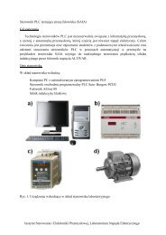


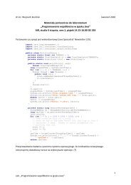


![[TCP] Opis układu - Instytut Sterowania i Elektroniki Przemysłowej ...](https://img.yumpu.com/23535443/1/184x260/tcp-opis-ukladu-instytut-sterowania-i-elektroniki-przemyslowej-.jpg?quality=85)