Linear Matrix Inequalities in Control
Linear Matrix Inequalities in Control
Linear Matrix Inequalities in Control

Create successful ePaper yourself
Turn your PDF publications into a flip-book with our unique Google optimized e-Paper software.
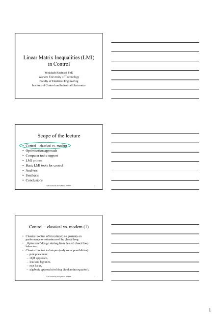
<strong>L<strong>in</strong>ear</strong> <strong>Matrix</strong> <strong>Inequalities</strong> (LMI)<br />
<strong>in</strong> <strong>Control</strong><br />
Wojciech Koz<strong>in</strong>ski PhD<br />
Warsaw University of Technology<br />
Faculty of Electrical Eng<strong>in</strong>eer<strong>in</strong>g<br />
Institute of <strong>Control</strong> and Industrial Electronics<br />
Scope of the lecture<br />
• <strong>Control</strong> – classical vs. modern<br />
• Optimisation approach<br />
• Computer tools support<br />
• LMI primer<br />
• Basic LMI tools for control<br />
• Analysis<br />
• Synthesis<br />
• Conclusions<br />
KSO materiały do wykładu 2008/09 2<br />
<strong>Control</strong> – classical vs. modern (1)<br />
• Classical control offers (almost) no guaranty on<br />
performance or robustness of the closed loop,<br />
• „Optimistic” design start<strong>in</strong>g from desired closed loop<br />
behaviour,<br />
• Classical control techniques (only some possibilities):<br />
– pole placement,<br />
– LQR approach,<br />
– lead and lag units,<br />
– root locus,<br />
– algebraic approach (solv<strong>in</strong>g diophant<strong>in</strong>e equation),<br />
KSO materiały do wykładu 2008/09 3<br />
1
<strong>Control</strong> – classical vs. modern (2)<br />
• Modern control techniques,<br />
– H analysis and synthesis,<br />
– H 2<br />
analysis and synthesis,<br />
– mixed criteria (+ pole placement),<br />
• They offer upper bounds estimates on performance and<br />
robustness of the closed loop,<br />
• They can tackle difficult problems,<br />
• Some disadvantages (high order controllers, a lot of<br />
mathematics, unable to solve some important problems).<br />
KSO materiały do wykładu 2008/09 4<br />
Scope of the lecture<br />
• <strong>Control</strong> – classical vs. modern<br />
• Optimisation approach<br />
• Computer tools support<br />
• LMI primer<br />
• Basic LMI tools for control<br />
• Analysis<br />
• Synthesis<br />
• Conclusions<br />
KSO materiały do wykładu 2008/09 5<br />
Optimisation approach (general)<br />
w<br />
p<br />
u<br />
Δ<br />
P<br />
K<br />
q<br />
y<br />
z<br />
x<br />
q<br />
y<br />
z<br />
u<br />
p<br />
Ax B1<br />
p B2w<br />
B3u<br />
C x D p D w D u<br />
q<br />
C x<br />
y<br />
Czx<br />
K y<br />
q<br />
D<br />
D<br />
q1<br />
y1<br />
z1<br />
p<br />
p<br />
q2<br />
D<br />
y2<br />
w<br />
D w D u<br />
z2<br />
q3<br />
z3<br />
f<strong>in</strong>d<br />
m<strong>in</strong><br />
K<br />
T<br />
zw p<br />
forall<br />
KSO materiały do wykładu 2008/09 6<br />
2
Optimisation approach (2)<br />
scalar signal norms<br />
L<br />
L 2<br />
norm - amplitude<br />
f ( t)<br />
sup f ( t)<br />
f<br />
t 0<br />
norm - energy<br />
1<br />
( d<br />
2<br />
2<br />
2<br />
f t)<br />
dt fˆ(<br />
)<br />
2<br />
0<br />
2<br />
KSO materiały do wykładu 2008/09 7<br />
Optimisation approach (3)<br />
system norm H<br />
System description (causal, with L 2 ga<strong>in</strong> γ>=0)<br />
x ( t)<br />
Ax(<br />
t)<br />
Bf ( t)<br />
y(<br />
t)<br />
Cx(<br />
t)<br />
Df ( t)<br />
H(<br />
s)<br />
C(<br />
sI<br />
Norm def<strong>in</strong>ition L 2 ga<strong>in</strong><br />
T<br />
T<br />
2<br />
2<br />
y(<br />
t)<br />
dt<br />
c<br />
0<br />
0<br />
H sup H(<br />
j<br />
R<br />
2<br />
f ( t)<br />
dt<br />
Norm <strong>in</strong>terpretation<br />
) H<br />
sup max<br />
R<br />
( H(<br />
j<br />
A)<br />
))<br />
1<br />
B<br />
D<br />
KSO materiały do wykładu 2008/09 8<br />
Optimisation approach (4)<br />
system norm H calculations<br />
Theorem<br />
Let A be a Hurwitz (stable) matrix. Then the L 2 ga<strong>in</strong> of the<br />
system is less than γ if and only if max(<br />
D)<br />
and the matrix<br />
F<br />
2<br />
A B(<br />
I<br />
T T<br />
C C C D(<br />
T 1 T<br />
D D)<br />
D C<br />
2 T 1 T<br />
I D D)<br />
D C<br />
2 T 1 T<br />
B(<br />
I D D)<br />
B<br />
T T 2 T<br />
A C D(<br />
I D D)<br />
1<br />
B<br />
does not have eigenvalues on the imag<strong>in</strong>ary axis.<br />
H<strong>in</strong>t : use bisection method.<br />
KSO materiały do wykładu 2008/09 9<br />
3
H<br />
2<br />
2<br />
Optimisation approach (5)<br />
– norm H 2<br />
If the <strong>in</strong>put <strong>in</strong>to system is white noise then output<br />
variance is called H 2 norm<br />
lim E y(<br />
t)<br />
t<br />
0<br />
2<br />
H<br />
If h(t) is impulse response matrix of the system, then<br />
T<br />
trace(<br />
h(<br />
t)<br />
h(<br />
t))<br />
dt<br />
2<br />
2<br />
1<br />
2<br />
T<br />
trace(<br />
H(<br />
j ) H(<br />
j )) d<br />
KSO materiały do wykładu 2008/09 10<br />
Optimisation approach (6)<br />
system norm calculations<br />
H 2<br />
Theorem:<br />
Let A be a Hurwitz matrix. The H 2 norm of the system is<br />
<strong>in</strong>f<strong>in</strong>ite if D 0.<br />
Otherwise, it equals:<br />
2<br />
T<br />
( ) trace T<br />
H trace CPC ( B QB)<br />
2<br />
Where P=P T and Q=Q T are the unique solutions of the<br />
Lapunov equations:<br />
AP<br />
T<br />
PA<br />
BB<br />
T<br />
T<br />
T<br />
0;<br />
A Q QA C C<br />
0<br />
KSO materiały do wykładu 2008/09 11<br />
Optimisation approach (7)<br />
<strong>L<strong>in</strong>ear</strong> Fractional Transformation (LFT)<br />
z1<br />
y1<br />
M<br />
l<br />
w1<br />
u1<br />
z1<br />
y<br />
u<br />
T<br />
1<br />
1<br />
zw1<br />
w1<br />
M<br />
u<br />
l<br />
y<br />
F<br />
1<br />
M<br />
M<br />
11<br />
21<br />
M<br />
M<br />
12<br />
22<br />
w1<br />
u<br />
1<br />
1<br />
l<br />
( M,<br />
l<br />
) M11<br />
M12<br />
l<br />
( I M22<br />
l<br />
) M21<br />
1<br />
z2<br />
y2<br />
u<br />
M<br />
u2<br />
w 2<br />
z2<br />
y<br />
u<br />
T<br />
2<br />
2<br />
zw2<br />
w2<br />
M<br />
u<br />
u<br />
F<br />
y<br />
2<br />
M<br />
M<br />
11<br />
21<br />
M<br />
M<br />
12<br />
22<br />
w2<br />
u<br />
2<br />
1<br />
u( M,<br />
u)<br />
M22<br />
M21<br />
u(<br />
I M11<br />
u)<br />
M12<br />
2<br />
KSO materiały do wykładu 2008/09 12<br />
4
Optimisation approach (8)<br />
Analysis - example<br />
w<br />
u<br />
e<br />
F C Go<br />
q<br />
Δ<br />
+<br />
p<br />
z<br />
-<br />
G<br />
0<br />
1<br />
; C<br />
2<br />
s<br />
F<strong>in</strong>d the largest<br />
2.35(1 s)<br />
;<br />
(1 0.1s<br />
)<br />
F<br />
1.2<br />
;<br />
s 1.2<br />
and ma<strong>in</strong>ta<strong>in</strong> stability<br />
KSO materiały do wykładu 2008/09 13<br />
Optimisation approach (9)<br />
Synthesis - example<br />
w<br />
-<br />
1<br />
s<br />
-<br />
10<br />
z<br />
Gi(s) G i<br />
( s)<br />
;<br />
2<br />
s as b<br />
x<br />
K a 1..3 ; b 8..12 ;<br />
For all plants G i (s) f<strong>in</strong>d stabilis<strong>in</strong>g<br />
static state space controller K.<br />
KSO materiały do wykładu 2008/09 14<br />
Optimisation approach (10)<br />
when the synthesis is well-posed?<br />
w<br />
u<br />
P(s)<br />
K(s)<br />
Closed loop description:<br />
cl<br />
y<br />
z<br />
x<br />
Ax B1w<br />
B2u<br />
z C1x<br />
D11w<br />
D12u<br />
y C x D w D u<br />
x f<br />
u<br />
2<br />
A x<br />
C x<br />
f<br />
f<br />
KSO materiały do wykładu 2008/09 15<br />
f<br />
f<br />
21<br />
D y<br />
22<br />
B y<br />
x A x B w x<br />
cl cl cl<br />
xcl<br />
z Cclxcl<br />
Dclw<br />
x<br />
f<br />
M<strong>in</strong>imize some measure ( T ) ( F ( P,<br />
K))<br />
w z<br />
l<br />
f<br />
f<br />
5
Optimisation approach (11)<br />
when the synthesis is well-posed?<br />
A<br />
C<br />
cl<br />
cl<br />
A B2D f<br />
C2<br />
B C<br />
C<br />
1<br />
f<br />
12<br />
2<br />
D D C<br />
f<br />
2<br />
B2C<br />
f<br />
A<br />
f<br />
D C ; D<br />
12<br />
; B<br />
f<br />
cl<br />
cl<br />
B1<br />
Df<br />
D<br />
B D<br />
D<br />
11<br />
f<br />
21<br />
12<br />
21<br />
D D D<br />
1. Simultanouos stabilisability of the pair (A,B 2 ) and observability of the pair<br />
(C 2 ,A).<br />
2. D-matrix conditions:<br />
1. D 22 =0,<br />
2. D cl =0 (if H 2 norm is used),<br />
3. often D 11 =0 required (Robust Toolbox),<br />
4. D 12 full column rank matrix,<br />
5. D 21 full row rank matrix.<br />
f<br />
21<br />
KSO materiały do wykładu 2008/09 16<br />
Optimisation approach (warn<strong>in</strong>g)<br />
• Many (all ?) control analysis and synthesis problems can be formulated<br />
as optimisation problems.<br />
• Only some of them can be transformed <strong>in</strong>to LMI (not BMI), solvable<br />
problems (e.g. there exists no general output controller synthesis for<br />
uncerta<strong>in</strong> plant – like LFT framework).<br />
• As LMI – the price is paid <strong>in</strong> large number of slack (Lapunov)<br />
variables.<br />
• Many <strong>in</strong>terest<strong>in</strong>g papers on BMI solvers and non-smooth, non-convex<br />
optimisation have been published recently. P.Apkarian ONERA-CERT,<br />
D. Noll Uni Toulouse, M.Overton, Uni of New York.<br />
KSO materiały do wykładu 2008/09 17<br />
Scope of the lecture<br />
• <strong>Control</strong> – classical vs. modern<br />
• Optimisation approach<br />
• Computer tools support<br />
• LMI primer<br />
• Basic LMI tools for control<br />
• Analysis<br />
• Synthesis<br />
• Conclusions<br />
KSO materiały do wykładu 2008/09 18<br />
6
Computer tools support<br />
• Matlab ® Robust <strong>Control</strong> Toolbox<br />
• Public doma<strong>in</strong> SDP-solvers (Matlab ® based):<br />
– SP (Boyd & Vanderberghe) –old,<br />
– SeDuMi (Sturm, now – McMaster University),<br />
• Public doma<strong>in</strong> preprocessors<br />
– YALMIP (Löfberg <strong>in</strong> ETH Zurich):<br />
• Many other possibilities (see YALMIP www<br />
page)<br />
KSO materiały do wykładu 2008/09 19<br />
Scope of the lecture<br />
• <strong>Control</strong> – classical vs. modern<br />
• Optimisation approach<br />
• Computer tools support<br />
• LMI primer<br />
• Basic LMI tools for control<br />
• Analysis<br />
• Synthesis<br />
• Conclusions<br />
KSO materiały do wykładu 2008/09 20<br />
F(<br />
x)<br />
LMI Primer (1) - def<strong>in</strong>ition<br />
LMI is a matrix dependent on vector x<br />
F<br />
0<br />
m<br />
i 1<br />
T<br />
z Fz<br />
x i<br />
F i<br />
0,<br />
z<br />
0<br />
where m<br />
x R , Fi<br />
Positive def<strong>in</strong>ite matrix F is such that<br />
0, z<br />
n<br />
R .<br />
n n<br />
If LMI has a solution (is feasible) then the solution is a<br />
non empty set. The solution set is convex.<br />
x|<br />
F(<br />
x)<br />
0<br />
KSO materiały do wykładu 2008/09 21<br />
R<br />
7
LMI Primer (2)<br />
There are many LMIs which have the same solution:<br />
Let M R<br />
n n<br />
; det( M)<br />
0 and x M z<br />
then by congruence can be obta<strong>in</strong>ed:<br />
T<br />
T T<br />
T<br />
A 0 x Ax 0 z M AMz 0 M AM<br />
An example:<br />
A B<br />
0<br />
C D<br />
0 I A B<br />
I 0 C D<br />
0 I<br />
0<br />
I 0<br />
D C<br />
0<br />
B A<br />
0<br />
KSO materiały do wykładu 2008/09 22<br />
LMI Primer (3)<br />
Multiple LMIs can be expressed as a s<strong>in</strong>gle LMI.<br />
Set def<strong>in</strong>ed by by q LMIs:<br />
F(<br />
x)<br />
1<br />
F ( x)<br />
2<br />
0; F ( x)<br />
An equivalent s<strong>in</strong>gle LMI:<br />
where<br />
q<br />
0;...; F ( x)<br />
m<br />
0<br />
xiFi<br />
x<br />
i 1<br />
F<br />
1 2<br />
q<br />
diag F ( x)<br />
F ( x)<br />
... F ( ) 0<br />
1 2<br />
q<br />
Fi diagFi<br />
Fi<br />
... Fi<br />
; i 0,1 ,..., m<br />
0<br />
KSO materiały do wykładu 2008/09 23<br />
LMI Primer (4)<br />
<strong>L<strong>in</strong>ear</strong> constra<strong>in</strong>ts can be expressed as an LMI:<br />
General l<strong>in</strong>ear constra<strong>in</strong>t:<br />
Ax<br />
b<br />
where<br />
n<br />
b R ,<br />
A<br />
R<br />
,<br />
n m<br />
x<br />
m<br />
R .<br />
can be converted to n scalar <strong>in</strong>equalities <strong>in</strong> LMI form<br />
m<br />
bi Aijx<br />
j<br />
0; i 1,...,<br />
n<br />
j 1<br />
and then <strong>in</strong>to s<strong>in</strong>gle LMI.<br />
KSO materiały do wykładu 2008/09 24<br />
8
LMI Primer (5)<br />
The Schur complement lemma:<br />
Converts convex nonl<strong>in</strong>ear <strong>in</strong>equality<br />
R(<br />
x)<br />
where<br />
0,<br />
Q(<br />
x)<br />
1 T<br />
S(<br />
x)<br />
R(<br />
x)<br />
S(<br />
x)<br />
T<br />
T<br />
Q( x)<br />
Q(<br />
x)<br />
, R(<br />
x)<br />
R(<br />
x)<br />
0 and S(<br />
x)<br />
<strong>in</strong>to the equivalent LMI<br />
Q(<br />
x)<br />
T<br />
S(<br />
x)<br />
S(<br />
x)<br />
R(<br />
x)<br />
Very important lemma!<br />
0<br />
0<br />
depend aff<strong>in</strong>ely on x<br />
KSO materiały do wykładu 2008/09 25<br />
The condition<br />
( A(<br />
x))<br />
1<br />
I<br />
A(<br />
x)<br />
T<br />
LMI Primer (6)<br />
Maximum s<strong>in</strong>gular value: is def<strong>in</strong>ed as:<br />
T<br />
( A(<br />
x))<br />
max(<br />
A(<br />
x)<br />
A(<br />
x)<br />
)<br />
where matrix A(x) depends aff<strong>in</strong>ely on x<br />
( A(<br />
x))<br />
1 can be expressed as a LMI<br />
A(<br />
x)<br />
A(<br />
x)<br />
A(<br />
x)<br />
0<br />
I<br />
T<br />
I I<br />
A(<br />
x)<br />
A(<br />
x)<br />
T<br />
0<br />
KSO materiały do wykładu 2008/09 26<br />
whereP<br />
LMI Primer (7)<br />
Algebraic Riccati <strong>in</strong>equality:<br />
T<br />
1 T<br />
A P PA PBR B P Q 0<br />
P<br />
T<br />
T<br />
0; Q Q ; R 0;<br />
can be expressed as a LMI<br />
T<br />
A P PA<br />
T<br />
B P<br />
Q<br />
PB<br />
R<br />
0;<br />
P<br />
0.<br />
KSO materiały do wykładu 2008/09 27<br />
9
LMI Primer (8)<br />
• Three types of LMI problems<br />
– feasibility problem LMIP,<br />
A(x) 0<br />
– eigenvalue problem EVP,<br />
m<strong>in</strong>imum c T x subject to A(x) 0<br />
– generalised eigenvalue problem GEVP,<br />
m<strong>in</strong>imum λ subject to A( x)<br />
B(<br />
x);<br />
B(<br />
x)<br />
0; C(<br />
x)<br />
where<br />
T<br />
T<br />
B ( x)<br />
B(<br />
x)<br />
0; A(<br />
x)<br />
A(<br />
x)<br />
0.<br />
KSO materiały do wykładu 2008/09 28<br />
Scope of the lecture<br />
• <strong>Control</strong> – classical vs. modern<br />
• Optimisation approach<br />
• Computer tools support<br />
• LMI primer<br />
• Basic LMI tools for control<br />
• Analysis<br />
• Synthesis<br />
• Conclusions<br />
KSO materiały do wykładu 2008/09 29<br />
Basic LMI tools for control (1)<br />
Stability<br />
Autonomous l<strong>in</strong>ear system<br />
x<br />
Ax<br />
T<br />
Lapunov function V( x)<br />
x Px 0 except x<br />
Condition on it’s derivative:<br />
dV(<br />
x)<br />
dt<br />
x Px<br />
T<br />
x Px<br />
T T<br />
x ( A P<br />
LMI for stability A T P PA<br />
0<br />
PA)<br />
x<br />
0<br />
P<br />
0<br />
T<br />
A P<br />
0<br />
PA<br />
0<br />
KSO materiały do wykładu 2008/09 30<br />
10
Basic LMI tools for control (2)<br />
Stability<br />
Equivalence between LMI def<strong>in</strong>ition and matrix formula<br />
p1<br />
p2<br />
Example for n=2 P<br />
0<br />
p p<br />
A T P PA<br />
2a<br />
p1<br />
a<br />
11<br />
12<br />
a12<br />
0<br />
a<br />
a<br />
11<br />
12<br />
a<br />
a<br />
21<br />
22<br />
11<br />
p1<br />
p<br />
2<br />
2<br />
2a21<br />
p2<br />
a a<br />
22<br />
p2<br />
p<br />
3<br />
3<br />
a11<br />
a<br />
2a<br />
12<br />
p1<br />
p<br />
2<br />
22<br />
p2<br />
p<br />
3<br />
a<br />
a<br />
11<br />
21<br />
0<br />
p3<br />
a<br />
21<br />
a<br />
a<br />
12<br />
22<br />
a<br />
2a<br />
21<br />
22<br />
KSO materiały do wykładu 2008/09 31<br />
Basic LMI tools for control (3)<br />
Stability<br />
Additional conditions on s-plane regions<br />
Guaranteed damp<strong>in</strong>g<br />
C stab<br />
{ s C | re(<br />
s)<br />
} s s 2 0<br />
Maximal damp<strong>in</strong>g and oscillation<br />
r s q<br />
C stab<br />
{ s C | s q r}<br />
0<br />
s q r<br />
Vertical strip<br />
( s s)<br />
2<br />
2<br />
0<br />
C stab<br />
{ s C |<br />
1<br />
re(<br />
s)<br />
2}<br />
0<br />
0 ( s s)<br />
2<br />
1<br />
KSO materiały do wykładu 2008/09 32<br />
Basic LMI tools for control (4)<br />
Stability<br />
Theorem:<br />
All eigenvalues of the real matrix A are <strong>in</strong> the region<br />
described by C<br />
stab<br />
{ s C|<br />
P Qs<br />
T<br />
Q s 0}<br />
with P<br />
T<br />
P<br />
if and only if there exists symmetric matrix X=X T >0<br />
p X<br />
p<br />
11<br />
k1<br />
X<br />
q11AX<br />
<br />
q AX<br />
k1<br />
T<br />
q11XA<br />
<br />
<br />
T<br />
q XA<br />
1k<br />
T<br />
p1<br />
k<br />
X q1<br />
k<br />
AX qk1XA<br />
<br />
T<br />
p X q AX q XA<br />
kk<br />
kk<br />
kk<br />
0<br />
Equivalent LMI us<strong>in</strong>g Kronecker multiplication:<br />
P X Q AX<br />
Q<br />
T<br />
XA<br />
T<br />
0<br />
KSO materiały do wykładu 2008/09 33<br />
11
Basic LMI tools for control (6)<br />
Stability – example - feasibility<br />
For given real matrix A check<br />
it its eigenvalues are <strong>in</strong>side<br />
the selected region:<br />
• usage of previously presented<br />
theorem,<br />
• feasibility type problem,<br />
r<br />
-4 -2<br />
q=-3<br />
Im<br />
1<br />
Re<br />
0<br />
-1<br />
KSO materiały do wykładu 2008/09 34<br />
Optimiser: SeDuMi<br />
Demo no.1<br />
Preprocesor: YALMIP<br />
Given is matrix A with eigenvalues -1 j1. If radius of the<br />
circle with orig<strong>in</strong> (-3,0) is greater then sqrt(5) the problem<br />
is feasible, otherwise unfeasible.<br />
KSO materiały do wykładu 2008/09 35<br />
Basic LMI tools for control (7)<br />
Stability of non-l<strong>in</strong>ear/time-vary<strong>in</strong>g<br />
Two admissible descriptions of autonomous non-l<strong>in</strong>ear<br />
or time vary<strong>in</strong>g system <strong>in</strong> form of convex hull of matrices:<br />
x t)<br />
A(<br />
t)<br />
x(<br />
t),<br />
A(<br />
t)<br />
Co{<br />
A,<br />
A ,... A }<br />
(<br />
1 2 L<br />
L<br />
x ( t)<br />
A(<br />
t)<br />
x(<br />
t),<br />
A(<br />
t)<br />
LMIs to prove stability:<br />
i<br />
A i<br />
i 1<br />
T<br />
P P 0<br />
T<br />
Ai P PAi<br />
0, i 1,...,<br />
L<br />
,<br />
i<br />
0,<br />
L<br />
i<br />
i 1<br />
1.<br />
KSO materiały do wykładu 2008/09 36<br />
12
Basic LMI tools for control (8)<br />
Bounded real lemma<br />
The system def<strong>in</strong>ition<br />
x Ax Bu<br />
G(<br />
s)<br />
sup ( G(<br />
s))<br />
sup ( G(<br />
j ))<br />
Re( s)<br />
0<br />
R<br />
y Cx Du<br />
x(0)<br />
0<br />
G(<br />
s)<br />
1<br />
C(<br />
sI A)<br />
B<br />
M<strong>in</strong>imize γ 2 subject to:<br />
T<br />
T<br />
T<br />
A P PA C C PB C D<br />
T T<br />
T 2<br />
B P D C D D I<br />
D<br />
F<strong>in</strong>d (the upper bound)<br />
0; P<br />
P<br />
T<br />
0<br />
KSO materiały do wykładu 2008/09 37<br />
Basic LMI tools for control (9)<br />
S-procedure (simplified)<br />
If there exist symmetric matrices T 0 ,...,T p and nonnegative<br />
numbers<br />
1<br />
0,...,<br />
p<br />
0 such that<br />
T<br />
0<br />
i<br />
p<br />
1<br />
iT i<br />
0<br />
T<br />
T<br />
then x T0 x 0; x 0if<br />
x Ti<br />
x 0; i 1, ,<br />
p.<br />
For p=1 the reverse is true.<br />
KSO materiały do wykładu 2008/09 38<br />
Basic LMI tools for control (10)<br />
S-procedure example<br />
There are two condtions given for P<br />
P<br />
T<br />
0,<br />
0 and any<br />
T<br />
T<br />
A P PA<br />
T<br />
B P<br />
PB<br />
0<br />
0<br />
T C T C<br />
T<br />
A P<br />
PA<br />
T<br />
B P<br />
T<br />
C C<br />
PB<br />
I<br />
0; P<br />
P<br />
T<br />
T .<br />
Us<strong>in</strong>g S-procedure one can obta<strong>in</strong> LMIs:<br />
0;<br />
0<br />
KSO materiały do wykładu 2008/09 39<br />
13
Basic LMI tools for control (11)<br />
H <strong>in</strong>f norm calculations<br />
For system:<br />
x<br />
y<br />
Ax<br />
Cx<br />
M<strong>in</strong>imize γ subject to:<br />
T<br />
A X XA<br />
T<br />
B X<br />
C<br />
XB<br />
I<br />
D<br />
T<br />
C<br />
T<br />
D<br />
I<br />
Bu<br />
Du<br />
0; X<br />
Variable γ is the upper bound of H <strong>in</strong>f<br />
0; whereX<br />
T<br />
X .<br />
KSO materiały do wykładu 2008/09 40<br />
Optimiser: SeDuMi<br />
Let<br />
G( s)<br />
2<br />
s<br />
10<br />
2s<br />
10<br />
Demo no.2<br />
The state space representation is<br />
A<br />
2<br />
8<br />
1.25<br />
; B<br />
0<br />
Preprocesor: YALMIP<br />
1<br />
; C<br />
0<br />
0 1.25; D 0.<br />
F<strong>in</strong>d norm H <strong>in</strong>f and compare it with the result of Matlab ®<br />
function.<br />
KSO materiały do wykładu 2008/09 41<br />
Basic LMI tools for control (12)<br />
H 2 norm calculations<br />
For system:<br />
x<br />
y<br />
Ax<br />
Cx<br />
Bu<br />
M<strong>in</strong>imize trace(Q) subject to:<br />
T T<br />
AP PA BB 0<br />
Q<br />
PC<br />
T<br />
whereP<br />
CP<br />
P<br />
T<br />
P , Q<br />
0; P<br />
0<br />
T<br />
Q .<br />
KSO materiały do wykładu 2008/09 42<br />
14
Optimiser: SeDuMi<br />
Demo no.3<br />
Preprocesor: YALMIP<br />
Let<br />
G( s)<br />
2<br />
s<br />
10<br />
2s<br />
10<br />
The state space representation is<br />
A<br />
2<br />
8<br />
1.25<br />
; B<br />
0<br />
1<br />
; C<br />
0<br />
0<br />
1.25; D<br />
0.<br />
F<strong>in</strong>d norm H 2 and compare it with the result of Matlab ®<br />
function.<br />
KSO materiały do wykładu 2008/09 43<br />
Scope of the lecture<br />
• <strong>Control</strong> – classical vs. modern<br />
• Optimisation approach<br />
• Computer tools support<br />
• LMI primer<br />
• Basic LMI tools for control<br />
• Analysis<br />
• Synthesis<br />
• Conclusions<br />
KSO materiały do wykładu 2008/09 44<br />
Analysis (1)<br />
Robustness problems<br />
1. Robust stability,<br />
2. Robust performance.<br />
Question: what is the biggest admissible Δ ?<br />
G G G 0<br />
( I )<br />
G 0<br />
Δ<br />
Δ<br />
G0<br />
G0<br />
KSO materiały do wykładu 2008/09 45<br />
15
Analysis (2)<br />
Uncerta<strong>in</strong>ity descriptions<br />
1. Norm-bounded uncerta<strong>in</strong>ity without structure<br />
1<br />
( s)<br />
W(<br />
s)<br />
2. Norm-bounded uncerta<strong>in</strong>ity with structure<br />
Δ partitioned <strong>in</strong>to blocks with their own bounds<br />
3. Sector-bounded uncerta<strong>in</strong>ity (dynamic or static)<br />
mapp<strong>in</strong>g : u L y L<br />
0<br />
( y(<br />
t)<br />
2<br />
T<br />
au(<br />
t))<br />
( y(<br />
t)<br />
2<br />
bu(<br />
t))<br />
dt<br />
1<br />
0<br />
KSO materiały do wykładu 2008/09 46<br />
Analysis (3)<br />
Robust stability – problem statement<br />
w<br />
p<br />
Δ<br />
P<br />
q<br />
z<br />
x<br />
q<br />
z<br />
p<br />
Ax B1<br />
p B2w<br />
C1x<br />
D11p<br />
D12w<br />
C2x<br />
D21p<br />
D22w<br />
q<br />
1<br />
Is the system stable for all admissible Δ?<br />
KSO materiały do wykładu 2008/09 47<br />
M<br />
1<br />
Analysis (3)<br />
Robust stability – LMIs<br />
T<br />
A P PA<br />
T<br />
B P<br />
PB<br />
0<br />
B<br />
B 1<br />
B 2<br />
M<br />
2<br />
C2<br />
0<br />
D<br />
0<br />
21<br />
T<br />
22<br />
D<br />
I<br />
I<br />
0<br />
0<br />
2<br />
I<br />
C2<br />
0<br />
D<br />
0<br />
21<br />
D<br />
I<br />
22<br />
M<br />
3<br />
C1<br />
D<br />
0 I<br />
11<br />
T<br />
D12<br />
I 0<br />
0 0 I<br />
C1<br />
D11<br />
D<br />
0 I 0<br />
m<strong>in</strong> s.<br />
t.(<br />
M1 M2<br />
M3<br />
0; P 0;<br />
12<br />
0)<br />
KSO materiały do wykładu 2008/09 48<br />
16
Analysis (4)<br />
Robust stability – example<br />
q Δ<br />
k<br />
w<br />
u<br />
e<br />
F C G o<br />
k<br />
p<br />
z<br />
2<br />
k<br />
q<br />
z<br />
2<br />
k G0C(<br />
I G0C)<br />
1<br />
k(<br />
I G C)<br />
0<br />
1<br />
kG0CF(<br />
I<br />
G CF(<br />
I<br />
0<br />
G0C)<br />
G C)<br />
0<br />
1<br />
1<br />
p<br />
w<br />
KSO materiały do wykładu 2008/09 49<br />
A<br />
C<br />
A<br />
Analysis (5)<br />
Robust stability – example<br />
G<br />
0<br />
C1<br />
C<br />
k max<br />
2<br />
0<br />
1<br />
; C<br />
2<br />
s<br />
B0Dr<br />
C<br />
BrC0<br />
0<br />
kC0<br />
C<br />
0<br />
0<br />
0.748<br />
B0Cr<br />
Ar<br />
0<br />
2.35(1 s)<br />
; F<br />
(1 0.1s<br />
)<br />
0 0<br />
; D<br />
0 0<br />
B0Dr<br />
C<br />
f<br />
BrC<br />
f<br />
A<br />
f<br />
D<br />
D<br />
11<br />
21<br />
; B<br />
D<br />
D<br />
12<br />
22<br />
1.2<br />
;<br />
s 1.2<br />
B0Dr<br />
k<br />
Brk<br />
0<br />
0<br />
k<br />
0<br />
0<br />
KSO materiały do wykładu 2008/09 50<br />
;<br />
B0Dr<br />
Df<br />
Br<br />
Df<br />
B<br />
f<br />
;<br />
Demo no.4<br />
Optimiser: SeDuMi<br />
Preprocesor: YALMIP<br />
Run the presented example with some simulations to<br />
confirm the result.<br />
KSO materiały do wykładu 2008/09 51<br />
17
Analysis (6)<br />
Integral Quadratic Constra<strong>in</strong>ts (IQC)<br />
Powerful method for <strong>in</strong>vestigat<strong>in</strong>g stability of uncerta<strong>in</strong> systems<br />
.<br />
Let pˆ and qˆ<br />
be Fourier Transforms of p and q signals.<br />
.<br />
IQC is def<strong>in</strong>ed by ( j ) where<br />
pˆ(<br />
j<br />
qˆ(<br />
j<br />
)<br />
)<br />
*<br />
( j<br />
pˆ(<br />
j<br />
)<br />
qˆ(<br />
j<br />
)<br />
d<br />
)<br />
0<br />
KSO materiały do wykładu 2008/09 52<br />
Analysis (7)<br />
Integral Quadratic Constra<strong>in</strong>ts (IQC)<br />
For autonomous system<br />
x<br />
( t)<br />
Ax(<br />
t)<br />
B p(<br />
t)<br />
q(<br />
t)<br />
p(<br />
t)<br />
C x(<br />
t)<br />
q<br />
q(<br />
t);<br />
p<br />
D p(<br />
t)<br />
qp<br />
01<br />
For small ε>0 it is true<br />
H(<br />
j )<br />
I<br />
*<br />
H(<br />
j )<br />
( j )<br />
I<br />
H(<br />
s)<br />
C ( sI<br />
1<br />
A)<br />
B<br />
KSO materiały do wykładu 2008/09 53<br />
q<br />
2 I for all<br />
Kalman-Yakubovich-Popov (KYP) lemma converts this<br />
condition <strong>in</strong>to LMI.<br />
R<br />
p<br />
D<br />
qp<br />
Analysis (8)<br />
Integral Quadratic Constra<strong>in</strong>ts (IQC)<br />
Kalman-Yakubovich-Popov (KYP) lemma:<br />
Let the pair of matrices (A,B) is stabilisable and matrix A has no<br />
eigenvalues on imag<strong>in</strong>ary axis. Then the statements are equivalent:<br />
( j<br />
1<br />
I A)<br />
B<br />
I<br />
T<br />
PA A P<br />
T<br />
B P<br />
*<br />
PB<br />
0<br />
( j<br />
1<br />
I A)<br />
B<br />
I<br />
0, P<br />
There is powerful Matlab ® toolbox called iqc-beta (from MIT).<br />
P<br />
T<br />
0,<br />
0<br />
0,<br />
KSO materiały do wykładu 2008/09 54<br />
18
Scope of the lecture<br />
• <strong>Control</strong> – classical vs. modern<br />
• Optimisation approach<br />
• Computer tools support<br />
• LMI primer<br />
• Basic LMI tools for control<br />
• Analysis<br />
• Synthesis<br />
• Conclusions<br />
KSO materiały do wykładu 2008/09 55<br />
Synthesis (1)<br />
What can be done with<strong>in</strong> LMI framework?<br />
• Design of static, state controller for uncerta<strong>in</strong><br />
plants with H 2 /H <strong>in</strong>f norm m<strong>in</strong>imization, pole<br />
placement,<br />
• Design of dynamic, output controller for nom<strong>in</strong>al<br />
plants with H 2 /H <strong>in</strong>f norm m<strong>in</strong>imization, pole<br />
placement,<br />
• Design of dynamic, output controller for uncerta<strong>in</strong><br />
plants with H 2 /H <strong>in</strong>f norm m<strong>in</strong>imization, pole<br />
placement, if uncerta<strong>in</strong>ity measurment is available<br />
(so called ga<strong>in</strong>-schedul<strong>in</strong>g).<br />
KSO materiały do wykładu 2008/09 56<br />
Synthesis (2)<br />
Typical strategy<br />
Pole placement and H <strong>in</strong>f +H 2 norms m<strong>in</strong>imisation,<br />
• Select the pole placement region and run the test to<br />
check, if it is feasible,<br />
• M<strong>in</strong>imise H <strong>in</strong>f norm to f<strong>in</strong>d the smallest possible one<br />
and controller,<br />
• For several, greater but fixed values of H <strong>in</strong>f norm<br />
m<strong>in</strong>imise H 2 norms,<br />
• Plot H 2 norms versus H <strong>in</strong>f fixed norms (Pareto like<br />
curve),<br />
• Select trade-off po<strong>in</strong>t or discard the design.<br />
KSO materiały do wykładu 2008/09 57<br />
19
Synthesis (3)<br />
Design of static, state controller<br />
w<br />
x<br />
z<br />
+<br />
u<br />
A x<br />
p<br />
C x<br />
p<br />
u Kx<br />
G<br />
K<br />
x<br />
B ( w<br />
p<br />
D ( w<br />
p<br />
z<br />
u)<br />
u)<br />
x<br />
z<br />
z<br />
z<br />
2<br />
w<br />
u<br />
KSO materiały do wykładu 2008/09 58<br />
P<br />
K<br />
x<br />
z2<br />
z<strong>in</strong>f<br />
z<br />
Ax Buu<br />
Bww<br />
C x D<br />
uu<br />
D<br />
ww<br />
C2x<br />
D2uu<br />
D2<br />
ww<br />
C x D u D w<br />
z<br />
zu<br />
zw<br />
2<br />
Synthesis (4)<br />
Design of static, state controller<br />
Norms def<strong>in</strong>itions (<strong>in</strong> signal terms)<br />
<strong>Matrix</strong> def<strong>in</strong>itions for general setup<br />
B<br />
C<br />
C<br />
C<br />
u<br />
z<br />
B ;<br />
p<br />
C ;<br />
Cp<br />
;<br />
0<br />
C ;<br />
p<br />
p<br />
B<br />
D<br />
w<br />
D<br />
D<br />
zu<br />
B ;<br />
u<br />
2u<br />
p<br />
D ;<br />
p<br />
D ;<br />
p<br />
Dp<br />
;<br />
1<br />
D<br />
zw<br />
D<br />
D<br />
w<br />
2w<br />
D ;<br />
p<br />
z w z;<br />
z2<br />
1 D ;<br />
p<br />
Dp<br />
;<br />
0<br />
z<br />
u<br />
KSO materiały do wykładu 2008/09 59<br />
Optimiser: SeDuMi<br />
G(<br />
s)<br />
1<br />
2<br />
s<br />
Demo no.5<br />
Preprocesor: YALMIP<br />
a) Pole placement and H <strong>in</strong>f m<strong>in</strong>imisation to obta<strong>in</strong> lower<br />
bound,<br />
b) Several runs – pole placement and H 2 m<strong>in</strong>imisation for<br />
fixed values H <strong>in</strong>f ,; generate Pareto-like curve,<br />
c) Pole placement and H <strong>in</strong>f + H 2 m<strong>in</strong>imisation.<br />
KSO materiały do wykładu 2008/09 60<br />
20
Synthesis (5)<br />
Design of static, state controller<br />
Analysis of the design (closed loop)<br />
x A x B w; x x; A A B K B B ;<br />
u<br />
z<br />
z<br />
z<br />
cl<br />
2<br />
cl<br />
cl<br />
cl<br />
K xcl;<br />
( C D<br />
uK)<br />
x<br />
( C2<br />
D2u<br />
K)<br />
xcl<br />
( C D K)<br />
x<br />
z<br />
zu<br />
cl<br />
If norm H 2 is used then<br />
cl<br />
cl<br />
D<br />
ww;<br />
D2<br />
ww;<br />
D w;<br />
D 2w<br />
zw<br />
0.<br />
cl<br />
;<br />
cl w<br />
KSO materiały do wykładu 2008/09 61<br />
u<br />
Synthesis (6)<br />
Design of static, state controller<br />
Another structure for uncerta<strong>in</strong> plants.<br />
w<br />
-<br />
e<br />
1/s<br />
v<br />
+<br />
u<br />
G<br />
K<br />
x<br />
z<br />
No problems with static ga<strong>in</strong>.<br />
KSO materiały do wykładu 2008/09 62<br />
Optimiser: SeDuMi<br />
Demo no.6<br />
10<br />
s)<br />
;<br />
s as b<br />
1..3 ; b 8..12 ;<br />
G i<br />
(<br />
2<br />
a<br />
Preprocesor: YALMIP<br />
Design state space controller for all „corner” plants<br />
us<strong>in</strong>g pole-placement.<br />
KSO materiały do wykładu 2008/09 63<br />
21
Synthesis (7)<br />
Design of dynamic, output controller<br />
w<br />
-<br />
u<br />
x Ax<br />
z Cx<br />
k<br />
x<br />
u<br />
Ak<br />
x<br />
C x<br />
k<br />
z<br />
G<br />
y<br />
Gk<br />
B(<br />
w u)<br />
D(<br />
w u)<br />
k<br />
k<br />
Bk<br />
y<br />
D y<br />
k<br />
w<br />
u<br />
P<br />
Gk<br />
z w z;<br />
z2<br />
y<br />
z<br />
u<br />
z2<br />
z<strong>in</strong>f<br />
z<br />
Design norms as an example<br />
KSO materiały do wykładu 2008/09 64<br />
Synthesis (8)<br />
Design of dynamic, output controller<br />
General design setup<br />
x<br />
Ax Buu<br />
Bww<br />
z C x D<br />
uu<br />
D<br />
ww<br />
z2<br />
C2x<br />
D2uu<br />
D2<br />
ww<br />
y C x D u D w<br />
z<br />
C x<br />
z<br />
y<br />
- H 2 norm<br />
yu<br />
D u<br />
D<br />
zu<br />
D D<br />
D<br />
yw<br />
zw<br />
w<br />
D<br />
2u<br />
k yw 2w<br />
D-matrix considerations:<br />
- well-posed feedback<br />
det( I D k<br />
Dyu)<br />
0<br />
- plant (usually) strictly proper<br />
D D yu<br />
0; D 0.<br />
0<br />
yw<br />
- well-posed optimization<br />
D w<br />
0;<br />
D2u<br />
0.<br />
- freedom to select<br />
0; D or D 0<br />
k<br />
0<br />
k<br />
KSO materiały do wykładu 2008/09 65<br />
Synthesis (9)<br />
Design of dynamic, output controller<br />
Structure of the closed loop and conversion rules:<br />
B B;<br />
B B;<br />
w<br />
z u<br />
w<br />
G<br />
C C;<br />
D D;<br />
D<br />
-<br />
u<br />
w<br />
u<br />
y C D<br />
Gk C2<br />
; D2u<br />
; D2<br />
w<br />
0 1<br />
Norms def<strong>in</strong>ed by:<br />
z w z;<br />
z2<br />
z<br />
u<br />
C<br />
C<br />
y<br />
z<br />
C;<br />
C;<br />
D<br />
D<br />
D;<br />
D;<br />
D;<br />
D;<br />
KSO materiały do wykładu 2008/09 66<br />
yu<br />
zu<br />
D<br />
D<br />
yw<br />
zw<br />
1;<br />
0<br />
0<br />
;<br />
22
Demo no.7<br />
Optimiser: SeDuMi<br />
Preprocesor: YALMIP<br />
1<br />
G(<br />
s)<br />
2<br />
s<br />
Design output, feedback controller us<strong>in</strong>g pole placement,<br />
and H <strong>in</strong>f + H 2 m<strong>in</strong>imisation.<br />
KSO materiały do wykładu 2008/09 67<br />
Synthesis (10)<br />
Design of dynamic, output controller<br />
Another closed loop structure and conversion rules<br />
w<br />
-<br />
y<br />
Gk<br />
u<br />
G<br />
Norms def<strong>in</strong>ed by:<br />
z w z;<br />
z2<br />
z<br />
u<br />
z<br />
Bu<br />
C<br />
C<br />
C<br />
C<br />
2<br />
y<br />
z<br />
B;<br />
Bw<br />
0;<br />
C;<br />
D<br />
C<br />
; D<br />
0<br />
C;<br />
D<br />
C;<br />
D<br />
zu<br />
u<br />
2u<br />
yu<br />
D;<br />
D<br />
D;<br />
D<br />
D;<br />
D<br />
zw<br />
2w<br />
yw<br />
w<br />
D<br />
; D<br />
1<br />
0;<br />
1;<br />
1;<br />
0<br />
;<br />
0<br />
KSO materiały do wykładu 2008/09 68<br />
Demo no.8<br />
Optimiser: SeDuMi<br />
Preprocesor: YALMIP<br />
G(<br />
s)<br />
1<br />
2<br />
s<br />
Design output, feedforward controller us<strong>in</strong>g pole placement,<br />
and H <strong>in</strong>f + H 2 m<strong>in</strong>imisation.<br />
KSO materiały do wykładu 2008/09 69<br />
23
Synthesis (11)<br />
H-<strong>in</strong>f loop shap<strong>in</strong>g<br />
z1<br />
W1<br />
w<br />
-<br />
y<br />
K<br />
u<br />
G<br />
d<br />
+<br />
W3<br />
z3<br />
z<br />
Basic idea:<br />
W1<br />
( s)<br />
S(<br />
s)<br />
W ( s)<br />
T(<br />
s)<br />
3<br />
1<br />
The sensitivity functions:<br />
L(<br />
s)<br />
S(<br />
s)<br />
T(<br />
s)<br />
G(<br />
s)<br />
K(<br />
s)<br />
( I<br />
( I<br />
G(<br />
s)<br />
K(<br />
s))<br />
1<br />
( I<br />
L(<br />
s))<br />
1<br />
G(<br />
s)<br />
K(<br />
s))<br />
G(<br />
s)<br />
K(<br />
s)<br />
I<br />
1<br />
S(<br />
s)<br />
( I<br />
1<br />
L(<br />
s))<br />
L(<br />
s)<br />
KSO materiały do wykładu 2008/09 70<br />
Optimisation setup:<br />
w<br />
m<strong>in</strong><br />
K<br />
u<br />
T<br />
P<br />
K<br />
w z<br />
Synthesis (12)<br />
H-<strong>in</strong>f loop shap<strong>in</strong>g<br />
y<br />
( s)<br />
z1<br />
z3<br />
z<br />
„Clever” selection of the<br />
z<strong>in</strong>f<br />
z1<br />
z3<br />
y<br />
x<br />
z<br />
y<br />
z<br />
w<br />
P<br />
u<br />
C x<br />
W1<br />
0<br />
I<br />
D u<br />
WG<br />
1<br />
W3G<br />
G<br />
Ax Buu<br />
Bww<br />
C x D<br />
uu<br />
D<br />
ww<br />
C x D u D w<br />
z<br />
y<br />
yu<br />
zu<br />
yw<br />
D w<br />
zw<br />
w<br />
u<br />
KSO materiały do wykładu 2008/09 71<br />
Demo no.9<br />
Optimiser: SeDuMi<br />
Preprocesor: YALMIP<br />
G ( s)<br />
1<br />
G ( s)<br />
2<br />
G ( s)<br />
3<br />
1 a<br />
2<br />
s ( s a)<br />
G0<br />
( I );<br />
1<br />
2 2<br />
2<br />
s ( s 2s<br />
)<br />
G0<br />
( I );<br />
1 s 1 b s<br />
e ;<br />
2<br />
2<br />
s s b s<br />
G0<br />
( I );<br />
filters W 1 and W 3<br />
1<br />
2<br />
2<br />
3<br />
KSO materiały do wykładu 2008/09 72<br />
( s)<br />
1<br />
( s)<br />
( s)<br />
3<br />
2<br />
s<br />
;<br />
s a<br />
2<br />
s 2s<br />
2<br />
s 2s<br />
2s<br />
;<br />
b s<br />
2<br />
;<br />
Design controller by the loop shap<strong>in</strong>g method tak<strong>in</strong>g <strong>in</strong>to<br />
account all possible neglected dynamics.<br />
24
Synthesis (13)<br />
Model predictive control (MPC)<br />
• For actual plant state x(k), f<strong>in</strong>d next M control u(k)<br />
steps (by optimisation), know<strong>in</strong>g next N (future)<br />
reference values. M
Demo no.10<br />
Optimiser: SeDuMi<br />
Preprocesor: YALMIP<br />
1. LQR control with control signal saturation<br />
(overshoot),<br />
2. MPC optimal control – no <strong>in</strong>put signal saturation,<br />
3. MPC control with <strong>in</strong>put signal saturation (LMI)<br />
KSO materiały do wykładu 2008/09 76<br />
Synthesis (16)<br />
Ga<strong>in</strong> Scheduled H-<strong>in</strong>f <strong>Control</strong>ler<br />
w<br />
p<br />
u<br />
?<br />
P(s)<br />
K(s)<br />
?<br />
y<br />
q<br />
z<br />
The plant description<br />
x<br />
A(<br />
) x B1<br />
( ) w B2<br />
( ) u<br />
z C1<br />
( ) x D11(<br />
) w D12(<br />
) u<br />
y C ( ) x D ( ) w<br />
A<br />
:<br />
R<br />
n<br />
2<br />
, D<br />
n<br />
1<br />
KSO materiały do wykładu 2008/09 77<br />
21<br />
p1<br />
m2<br />
12<br />
R ,<br />
<br />
T<br />
L<br />
D<br />
The unknown parametres form<br />
a hypercube<br />
( t)<br />
, t<br />
i<br />
i<br />
i<br />
0<br />
21<br />
R<br />
p2<br />
m1<br />
Synthesis (17)<br />
Ga<strong>in</strong> Scheduled H-<strong>in</strong>f <strong>Control</strong>ler<br />
w<br />
p<br />
u<br />
?<br />
P(s)<br />
K(s)<br />
?<br />
y<br />
q<br />
z<br />
F<strong>in</strong>d a dynamic controller<br />
x<br />
u<br />
K<br />
AK<br />
( ) x<br />
C ( ) x<br />
K<br />
K<br />
K<br />
BK<br />
( ) y<br />
D ( ) y<br />
which ensures <strong>in</strong>ternal stability<br />
and a guaranteed L 2<br />
-ga<strong>in</strong><br />
T<br />
0<br />
T<br />
z zd<br />
T<br />
2 T<br />
0<br />
K<br />
w wd ,<br />
T<br />
0<br />
KSO materiały do wykładu 2008/09 78<br />
26
Synthesis (18)<br />
Ga<strong>in</strong> Scheduled H-<strong>in</strong>f <strong>Control</strong>ler<br />
• Ga<strong>in</strong> scheduled H-<strong>in</strong>f controller can be<br />
calculated <strong>in</strong> three steps:<br />
1. After the application of elim<strong>in</strong>ation lemma one can<br />
obta<strong>in</strong> Lapunov matrices X and Y for all vertices of<br />
hypercube.<br />
2. For each vertex of hypercube calculate the vertex<br />
controller.<br />
3. For each value of parameter calculate the<br />
correspond<strong>in</strong>g controller and use it <strong>in</strong> the control.<br />
KSO materiały do wykładu 2008/09 79<br />
Synthesis (19)<br />
Elim<strong>in</strong>ation Lemma<br />
• Def<strong>in</strong>ition. An orthogonal complement of given<br />
matrix N is any maximal rank matrix, such that<br />
T<br />
N N 0 and N N 0.<br />
n k n m<br />
T n n<br />
• Lemma. Let M R , N R , H H R<br />
The follow<strong>in</strong>g statements are equivalent:<br />
m k<br />
1. There exists X R such that<br />
T T T<br />
NXM MX N H 0<br />
2. The follow<strong>in</strong>g two conditions hold<br />
N HN<br />
T<br />
M HM<br />
T<br />
0<br />
0<br />
KSO materiały do wykładu 2008/09 80<br />
Synthesis (20)<br />
Ga<strong>in</strong> Scheduled H-<strong>in</strong>f <strong>Control</strong>ler<br />
Step 1. Solve 2*2 L +1 LMIs for X and Y Lapunov matrices<br />
NX<br />
0<br />
0<br />
I<br />
T<br />
T<br />
XA A X<br />
T<br />
B1<br />
X<br />
C<br />
1<br />
XB1<br />
I<br />
D<br />
11<br />
T<br />
C1<br />
T<br />
D11<br />
I<br />
NX<br />
0<br />
0<br />
I<br />
0<br />
Where:<br />
N X<br />
null( C 2<br />
D21<br />
)<br />
)<br />
NY<br />
0<br />
0<br />
I<br />
T<br />
T<br />
YA AY<br />
C Y<br />
B<br />
1<br />
T<br />
1<br />
T<br />
YC1<br />
I<br />
D<br />
T<br />
11<br />
B1<br />
D11<br />
I<br />
NY<br />
0<br />
0<br />
I<br />
0<br />
N<br />
Y<br />
null<br />
T T<br />
( B2<br />
D12<br />
X<br />
I<br />
I<br />
Y<br />
0<br />
KSO materiały do wykładu 2008/09 81<br />
27
Synthesis (21)<br />
Ga<strong>in</strong> Scheduled H-<strong>in</strong>f <strong>Control</strong>ler<br />
Step 2. Calculate controller for each vertex of hypercube<br />
by solv<strong>in</strong>g LMI. Some constra<strong>in</strong>ts can be added.<br />
XCl<br />
0<br />
T<br />
T T<br />
XCl<br />
0<br />
P KQ Q K P<br />
0 I<br />
0 I<br />
0<br />
where:<br />
AK<br />
B I X Y I<br />
K<br />
K<br />
XCl<br />
T T<br />
C D 0 M N 0<br />
MN T I YX<br />
0<br />
K<br />
A0<br />
X<br />
Cl<br />
X<br />
Cl<br />
A0<br />
T<br />
B0<br />
X<br />
Cl<br />
C<br />
K<br />
XClB0<br />
I<br />
D<br />
NB: Not all symbols are def<strong>in</strong>ed (see next slide).<br />
11<br />
T<br />
C0<br />
T<br />
T<br />
D11<br />
; P B 0 D12<br />
; Q C D21<br />
I<br />
KSO materiały do wykładu 2008/09 82<br />
0<br />
Synthesis (22)<br />
Ga<strong>in</strong> Scheduled H-<strong>in</strong>f <strong>Control</strong>ler<br />
Step 2. (cont<strong>in</strong>ued)<br />
Extended plant parameters<br />
A 0 B1<br />
0<br />
A0<br />
; B0<br />
; B<br />
0 0 0 I<br />
D<br />
12<br />
0<br />
k<br />
D ; D<br />
12<br />
k<br />
21<br />
0<br />
D<br />
21<br />
Closed loop description<br />
A<br />
C<br />
Cl<br />
Cl<br />
B<br />
D<br />
Cl<br />
Cl<br />
A0<br />
C<br />
0<br />
B0<br />
D<br />
11<br />
;<br />
k<br />
B<br />
D<br />
12<br />
k<br />
B2<br />
; C0<br />
0<br />
A<br />
C<br />
K<br />
K<br />
BK<br />
D<br />
K<br />
C<br />
C<br />
1<br />
0 ; C<br />
D<br />
21<br />
0<br />
C<br />
2<br />
Ik<br />
k<br />
;<br />
0<br />
KSO materiały do wykładu 2008/09 83<br />
Synthesis (23)<br />
Ga<strong>in</strong> Scheduled H-<strong>in</strong>f <strong>Control</strong>ler<br />
Step 3. <strong>Control</strong>ler for given value of parameter.<br />
Case of one parameter:<br />
( t)<br />
, t<br />
There are two controllers<br />
0<br />
K and K<br />
For given value of parameter θ<br />
;<br />
0<br />
1<br />
K (1 )K<br />
K<br />
Extension for multiparameter case. Possible simplifications.<br />
KSO materiały do wykładu 2008/09 84<br />
28
Optimiser: SeDuMi<br />
Demo no.11<br />
Preprocesor: YALMIP<br />
For the plant with measurable, time-vary<strong>in</strong>g parameter a<br />
design the ga<strong>in</strong> schedul<strong>in</strong>g controller.<br />
1<br />
G( s)<br />
; a 1.0 <br />
s(<br />
s a)<br />
1.0<br />
KSO materiały do wykładu 2008/09 85<br />
Scope of the lecture<br />
• <strong>Control</strong> – classical vs. modern<br />
• Optimisation approach<br />
• Computer tools support<br />
• LMI primer<br />
• Basic LMI tools for control<br />
• Analysis<br />
• Synthesis<br />
• Conclusions<br />
KSO materiały do wykładu 2008/09 86<br />
Conclusions<br />
• New (~15 years old) control analysis and control synthesis<br />
tool,<br />
• Active field of research with many unsolved problems:<br />
– BMI as natural formulation of control problems,<br />
but not convex,<br />
– suboptimal, low order controllers, controllers with structure (nonsmooth,<br />
non-convex algorithms).<br />
– output controllers for uncerta<strong>in</strong> plants,<br />
– synthesis for systems with delays, saturations,<br />
KSO materiały do wykładu 2008/09 87<br />
29
Thank you for your attention!<br />
KSO materiały do wykładu 2008/09 88<br />
30


![[TCP] Opis układu - Instytut Sterowania i Elektroniki Przemysłowej ...](https://img.yumpu.com/23535443/1/184x260/tcp-opis-ukladu-instytut-sterowania-i-elektroniki-przemyslowej-.jpg?quality=85)