Variance Estimation for the General Regression Estimator

6
⎧
⎨
⎪
⎢
⎩⎣
⎪
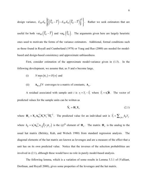
design variance,
ˆ
ˆ
( ) ( ) 2
E E ⎡ Y Y E E Y Y ⎤
− − −
M π G M π G
useful for both var
ˆ
M ( Y G − Y)
and var
ˆ
π ( Y G)
⎥⎦
⎫⎪
⎬. Rather we seek estimators that are
⎪⎭
. The arguments given here are largely heuristic
ones used to motivate the forms of the variance estimators. Additional, formal conditions such
as those found in Royall and Cumberland (1978) or Yung and Rao (2000) are needed for modelbased
and design-based consistency and approximate unbiasedness.
First, consider estimation of the approximate model-variance given in (1.5). In the
following development, we assume that, as N and n become large,
(i) Nmax( ) O( n)
i
π = and
i
(ii) A πs N converges to a matrix of constants, A o.
A residual associated with sample unit i is
r = Y − Yˆ
where Y ˆ =xB. ′ ˆ The vector of
i i i
i
i
predicted values for the sample units can be written as
Yˆs = HY s s
(2.1)
where
1 1 1
s = s π − s ′ s s − s
−
=∑ ∈
H XA XV Π . The predicted value for an individual unit is Y ˆi hY ij j
j s
1
where hij ′
−
i πs j ( vjπ
j)
=xA x is the (ij) th element of H s. The matrix
H s is the analog to the
usual hat matrix (Belsley, Kuh, and Welsch 1980) from standard regression analysis. The
diagonal elements of the hat matrix are known as leverages and are a measure of the effect that a
unit has on its own predicted value. Notice that the inverses of the selection probabilities are
involved in (2.1), although these would have no role in purely model-based analysis.
The following lemma, which is a variation of some results in Lemma 5.3.1 of (Valliant,
Dorfman, and Royall 2000), gives some properties of the leverages and the hat matrix.