CHAPTER 9 ANALYSIS EXAMPLES REPLICATION-R SURVEY ...
CHAPTER 9 ANALYSIS EXAMPLES REPLICATION-R SURVEY ...
CHAPTER 9 ANALYSIS EXAMPLES REPLICATION-R SURVEY ...

Create successful ePaper yourself
Turn your PDF publications into a flip-book with our unique Google optimized e-Paper software.
<strong>CHAPTER</strong> 9 <strong>ANALYSIS</strong> <strong>EXAMPLES</strong> <strong>REPLICATION</strong>-R <strong>SURVEY</strong> PACKAGE 3.22<br />
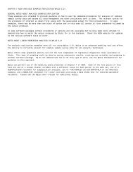
GENERAL NOTES ABOUT <strong>ANALYSIS</strong> <strong>EXAMPLES</strong> <strong>REPLICATION</strong><br />
These examples are intended to provide guidance on how to use the commands/procedures for analysis of complex<br />
sample survey data and assume all data management and other preliminary work is done. The relevant syntax for<br />
the procedure of interest is shown first along with the associated output for that procedure(s). In some<br />
examples, there may be more than one block of syntax and in this case all syntax is first presented followed by<br />
the output produced.<br />
In some software packages certain procedures or options are not available but we have made every attempt to<br />
demonstrate how to match the output produced by Stata 10+ in the textbook. Check the ASDA website for updates<br />
to the various software tools we cover.<br />
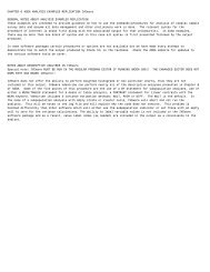
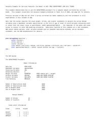
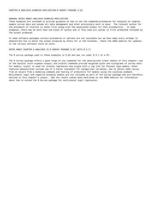
NOTES ABOUT <strong>CHAPTER</strong> 9 ANALYSES IN R <strong>SURVEY</strong> PACKAGE 3.22 (WITH R 2.7)<br />
The R survey package used in these examples is 3.22 and was run under R 2.7 on a PC.<br />
The R survey package offers a good range of svy commands for the generalized linear models of this chapter: use<br />
of the barplot (with svymean output) and svyhist commands provide weighted plots and histograms of survey data.<br />
For models, svyolr is used for ordinal regression and svyglm with a log link for Poisson type models. Other<br />
features demonstrated include use of a factor statement for categorical variables, how to obtain odds ratios<br />
from an object from a modeling command and testing of predictors for models using the svychisq command.<br />
Multinomial logit and negative binomial models are not included as part of the survey package and are therefore<br />
omitted in this chapter’s output. See the recent Lumley book mentioned on the ASDA website for information<br />
about how to extend the R Survey package for multinomial logit regression.
#Data production and set up of design objects<br />
#remember to load package first survey package<br />
#NHANES<br />
nhanesdata
0.0 0.1 0.2 0.3 0.4 0.5 0.6<br />
#FIGURE 9.1 BAR CHART OF WORK STATUS NCS-R DATA<br />
fig91
#BIVARIATE TESTING PRIOR TO MULTINOMIAL LOGIT<br />
>svychisq(~WKSTAT3C+SEX, ncsrsvyp2, statistic="F")<br />
Pearson's X^2: Rao & Scott adjustment<br />
data: svychisq(~WKSTAT3C + SEX, ncsrsvyp2, statistic = "F")<br />
F = 27.3292, ndf = 1.875, ddf = 78.748, p-value = 2.171e-09<br />
> svychisq(~WKSTAT3C+ald, ncsrsvyp2, statistic="F")<br />
Pearson's X^2: Rao & Scott adjustment<br />
data: svychisq(~WKSTAT3C + ald, ncsrsvyp2, statistic = "F")<br />
F = 3.1249, ndf = 1.725, ddf = 72.441, p-value = 0.05716<br />
> svychisq(~WKSTAT3C+mde, ncsrsvyp2, statistic="F")<br />
Pearson's X^2: Rao & Scott adjustment<br />
data: svychisq(~WKSTAT3C + mde, ncsrsvyp2, statistic = "F")<br />
F = 4.6693, ndf = 1.735, ddf = 72.861, p-value = 0.01605<br />
> svychisq(~WKSTAT3C+ED4CAT, ncsrsvyp2, statistic="F")<br />
Pearson's X^2: Rao & Scott adjustment<br />
data: svychisq(~WKSTAT3C + ED4CAT, ncsrsvyp2, statistic = "F")<br />
F = 27.6404, ndf = 5.146, ddf = 216.118, p-value < 2.2e-16<br />
> svychisq(~WKSTAT3C+MAR3CAT, ncsrsvyp2, statistic="F")<br />
Pearson's X^2: Rao & Scott adjustment<br />
data: svychisq(~WKSTAT3C + MAR3CAT, ncsrsvyp2, statistic = "F")<br />
F = 23.1237, ndf = 3.198, ddf = 134.337, p-value = 1.229e-12<br />
> svychisq(~WKSTAT3C+ag4cat, ncsrsvyp2, statistic="F")<br />
Pearson's X^2: Rao & Scott adjustment<br />
data: svychisq(~WKSTAT3C + ag4cat, ncsrsvyp2, statistic = "F")<br />
F = 113.4945, ndf = 4.965, ddf = 208.513, p-value < 2.2e-16<br />
# MULTINOMIAL LOGISTIC IS NOT AVAILABLE IN <strong>SURVEY</strong> PACKAGE OF R, SEE THE EXTENSION OF THE <strong>SURVEY</strong> R PACKAGE IN THE<br />
APPENDIX OF LUMLEY’S BOOK ABOUT HOW TO POSSIBLY EXTEND THE PACKAGE
0.00 0.05 0.10 0.15 0.20 0.25 0.30<br />
#FIGURE 9.2 BAR CHART OF SELF RATED HEALTH HRS DATA<br />
> fig92 barplot(fig92, legend=c("Excellent", "Very Good", "Good", "Fair", "Poor") , col=c("black", "grey60", "blue",<br />
"red", "green"))<br />
Excellent<br />
Very Good<br />
Good<br />
Fair<br />
Poor<br />
factor(selfrhealth)1 factor(selfrhealth)2 factor(selfrhealth)3 factor(selfrhealth)4 factor(selfrhealth)5
#ORDINAL LOGISTIC REGRESSION USING HRS DATA<br />
> summary(ex92_ordinal exp(ex92_ordinal$coef)<br />
male KAGE<br />
0.9317625 1.0292298
Density<br />
0.00 0.05 0.10 0.15<br />
#HISTOGRAM OF NUMBER OF FALLS DURING PAST 24 MONTHS HRS DATA<br />
svyhist(~numfalls24 , subset (hrssvyr, KAGE >=65), main="", col="grey80", xlab ="Histogram of Number of Falls<br />
Past 24 Months")<br />
0 10 20 30 40 50<br />
Histogram of Number of Falls Past 24 Months
#EXAMPLE 9.3 POISSON MODEL NUMBER OF FALLS DURING PAST 24 MONTHS HRS DATA<br />
> ex93_poisson summary(ex93_poisson)<br />
Call:<br />
svyglm(numfalls24 ~ male + factor(age3cat) + arthritis + DIABETES +<br />
bodywgt + totheight, design = hrssvyr, family = quasipoisson(log))<br />
Survey design:<br />
svydesign(strata = ~STRATUM, id = ~SECU, weights = ~KWGTR, data = hrs,<br />
nest = T)<br />
#NOTE: CODES FOR AGE3CAT 1=65-74 2=75-84 3=85+ YEARS OF AGE<br />
Coefficients:<br />
Estimate Std. Error t value Pr(>|t|)<br />
(Intercept) 0.4938245 0.6359374 0.777 0.441499<br />
male 0.1831258 0.1073485 1.706 0.094921 .<br />
factor(age3cat)2 0.2383983 0.0534633 4.459 5.43e-05 ***<br />
factor(age3cat)3 0.5838654 0.0899710 6.489 5.84e-08 ***<br />
arthritis 0.4867153 0.0824179 5.905 4.31e-07 ***<br />
DIABETES 0.2596115 0.0689276 3.766 0.000478 ***<br />
bodywgt 0.0009237 0.0008851 1.044 0.302200<br />
totheight -0.0224337 0.0110317 -2.034 0.047917 *<br />
---<br />
Signif. codes: 0 ‘***’ 0.001 ‘**’ 0.01 ‘*’ 0.05 ‘.’ 0.1 ‘ ’ 1<br />
(Dispersion parameter for quasipoisson family taken to be 3.052147)<br />
Number of Fisher Scoring iterations: 6<br />
> exp(ex93_poisson$coef)<br />
(Intercept) male factor(age3cat)2 factor(age3cat)3 arthritis DIABETES bodywgt<br />
1.638571 1.200965 1.269215 1.792955 1.626963 1.296426 1.000924<br />
totheight<br />
0.977816
# NEGATIVE BINOMIAL (NOT AVAILABLE WITH <strong>SURVEY</strong> CORRECTION, DISPERSION IS ACCOUNTED FOR IN SVYGLM, PER LUMLEY)<br />
# ZERO INFLATED NEGATIVE BINOMIAL NOT AVAILABLE IN R <strong>SURVEY</strong> PACKAGE