SOFC Modeling - From Micro-Kinetics to Stacks - KIT

A0201 – Abstract A021 – Oral Presentation – Session A02 – Modeling Sesson – Tuesday, July 1, 2008 – 11:00 h 

SOFC Modeling - From Micro-Kinetics to Stacks 

Olaf Deutschmann, Vinod Janardhanan, Steffen Tischer, Vincent Heuveline 

Universität Karlsruhe (TH) 

Institute for Chemical Technology & Polymer Chemistry 

Engesserstr. 20 

76131 Karlsruhe, Germany 

Tel: +49-721-608 3138 

olaf.deutschmann@kit.edu 

Abstract 

This paper presents a hierarchical modeling approach for Solid-Oxide Fuel Cells from 

elementary kinetics to stacks. On a fundamental level, we have developed an analytical 

model for the evaluation of volume specific three-phase boundary length (vL tpb ) in 

composite electrodes and electrochemical kinetics expressions to account for coverage 

dependent activation energies of various surface adsorbed species. The kinetics are 

applied for modeling SOFCs operating on various reformate compositions. The results of 

both fundamental modeling approaches are compared with experimental data [1, 2]. On 

an application level, a novel approach for modeling a SOFC stack is presented. The 

approach is based on decoupling heat transfer from the other processes [3] and a newly 

developed cluster agglomeration algorithm, which drastically reduces the computational 

costs associated with stack simulation. Based on the assumption that all unit cells with 

similar temperature profiles behave alike, the cells are divided into clusters according to 

differences in their local temperature profiles. All unit cells of one cluster are then 

represented by one cell, for which a simulation is conducted, which applies detailed 

models for electro-chemical conversion at the three-phase boundary, an elementary-step 

reaction mechanism for the thermo-catalytic conversion of the fuel on the catalyst in the 

anode [4], dusty-gas model to account for multi-component diffusion and convection in the 

electrodes, and a plug-flow model for the flow in the fuel and air channels. 

1. Introduction 

Currently SOFCs running on multi-component fuel mixtures are receiving special attention 

[5-9]. Extensive research has been subjected to run diesel or gasoline reformate on 

SOFCs. However, these reformate will essentially be a fuel mixture of hydrocarbons and 

syngas [10, 11]. Depending on the conditions in the fuel reformer, CO 2 /H 2 O can also be 

present in the reformate fuel. Under these circumstances, the accuracy of an SOFC model 

depends largely on coupled interactions of heterogeneous chemistry and electrochemistry. 

Although SOFC numerical models can throw great insight into details of physico-chemical 

processes occurring in the cell, the performance of the cell largely depends on the 

materials, manufacturing conditions, and the resulting microstructure of the cell 

components. In-order to cover the aspects ranging from microstructures to stacks, this 

paper is organized into three major sections namely (1) electrode micro-structure, (2) 

heterogeneous charge transfer model, and (3) stack model. 

1


2. Electrode microstructure 

The performance of an SOFC largely depends on the microstructure of the resulting 

electrodes and the processing conditions. The electrochemical charge transfer reactions 

proceeds at the three-phase interfaces (TPB). In a composite electrode, normally the 

active TPB region spreads to a few microns (10-15 µm) in the vicinity of electrodeelectrolyte 

interface. Wilson et al. [1] reported the three-dimensional reconstruction of a 

SOFC anode using ion-beam scanning electron microscopy to determine the microstructural 

properties. They estimated the volume-specific TPB length for their sample to be 

4.28×10 12 m/m 3 . Brown et al. [12] reported that Ni forms larger particles with the particle 

sizes ranging from 0.5 to 3.0 μm, while YSZ phase particle size distribution were 0.5-1.0 

μm. Hence, we need to consider the volume specific TPB length for cases with two monosized 

particle distributions. Schneider et al. [13] reported the discrete modeling of 

composite electrode and developed an analytical model for calculating the TPB length. 

The model presented here is developed by considering a geometric volume of a composite 

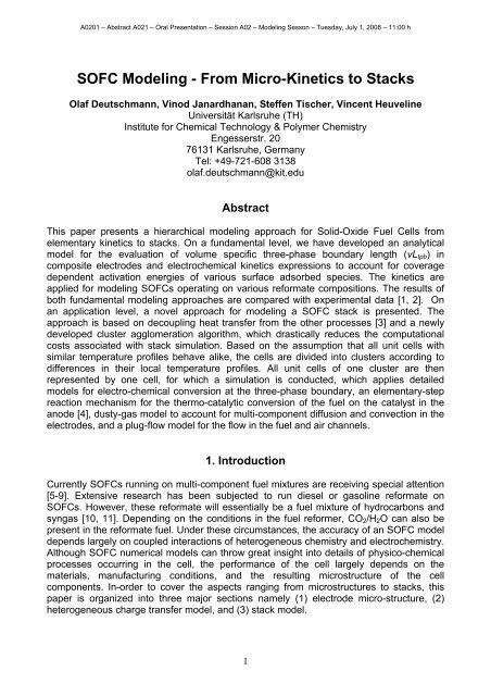
electrode characterized by its porosity and particle radii r 1 and r 2 . We start the model 

development by considering the intersection of two spherical particles as shown in Fig 1. 

Figure 1: Intersection of two spherical particles. 

The volume of the three dimensional lens common to both the spheres as a result of 

intersection is given by 

V 

l 

2 2 2 2 

π ( r1+ r2 − d) ( d + 2dr2 − 3r2 + 2dr1+ 6rr 2 1−3 r1 

) 

= . (1) 

12d 

Further the intersection of the spheres is a curve lying in the plane parallel to the x-plane 

whose radius a is given by 

1 2 2 2 2 2 2 

a= 4 d r1 −( d − r2 + r1 

) . (2) 

2d 

The total volume loss V 

tl 

as a result of intersection is given by 

2


V = N (1 − ψ ) V . (3) 

tl p l 

Here, ψ is the fractional overlap and N 

p 

is the number of particles. If we assume the 

electronic and ionic particles are of different average sizes with radii r 1 

and r 

2 

, then the 

ratio between the number of particles M can be defined as 

M 

N 

3 

p2 

φ2r1 

= = 

(4) 

3 

N 

p1 

φ1r2 

with φ 1 and φ 2 as volume fraction of particles with radii r 1 and r 2 , respectively. Let V 

t 

be the 

total volume of the electrode under consideration then, the total solid volume V t 

can be 

expressed as 

4 3 4 3 

(1 − φ) Vt = Np 1 

πr1 + Np2 πr2 − ( Np 1+ Np2)(1 − ψ) 

Vl, (5) 

3 3 

φ is the gas-phase porosity. Combining the above equations, the total number of particles 

can be written as 

N 

p 

= 

(1 − φ) Vt 

(1 + M) 

4 ( 

3 3 

π r1 + Mr2 

) − (1 − ψ )(1 + M ) Vl 

3 

. (6) 

The length of boundary due to the intersection of two spheres is given by the 

circumference of a circle. This becomes a three-phase boundary length (TPB) only if the 

intersecting particles are of different phases and the intersection is associated with a pore 

space. Therefore, the average TPB length of the composite electrode is given by 

L = N min Z , Z φ2π 

a, (7) 

tpb p i−e e−i 

Zi − eis the coordination number between the ionic and electronic conductors and Ze − iis the 

coordination number between the electronic and ionic conductors. The average number of 

contacts between the ionic and electronic conducting particle is given by 

Z 

Z Z 

Z 

= i e 

i− e 

φ , (8) 

e 

and the average number of contacts between the electronic and ionic conducting particle 

is given by 

ZiZe 

Z = e− i 

φi 

Z 

. (9) 

Here, Z is the average co-ordination number. Expressions for Z 

i 

and Ze 

are given in [14]. 

Combination of Eqs. (6) and (7) leads to the volume specific three-phase boundary length 

vL : 

tpb 

3


vL 

tpb 

φ(1 − φ)(1 + M ) min Zi−e, Ze−i 

2πa 

= 

. (10) 

4 ( 

3 3 

π r1 + Mr2 

) − (1 − ψ )(1 + M ) Vl 

3 

In the case of mono-sized particles 

vLtpb 

is given by 

vL 

tpb 

φ(1 −φ) min Zi−e, Ze−i 

2πa 

= 

. (11) 

4 3 

πr 

−(1 −ψ) 

Vl 

3 

The model presented here is developed by considering a geometric volume of a composite 

electrode characterized by its porosity φ and particle radii r 1 and r 2 . It is assumed that the 

ionic and electronic solid phases are made up of spherical particles. 

3. Heterogeneous charge transfer model 

Most SOFC modeling efforts employ Nernst equation to calculate the open circuit potential 

and Butler-Volmer equation to express the rate of charge transfer reaction. However, 

Butler-Volmer equation does not throw any insight into the actual process occurring on the 

surface which leads to electron transfer near the TPB. Here we present an 

electrochemistry model based on heterogeneous chemistry occurring at the TPB. A 

detailed version of the following discussions will be published elsewhere [15]. 

The forward and reverse rate constants for charge transfer reaction are written as 

α 

0 aF 

kfi 

= kfi 

exp( z Δ φ) 

and (12) 

RT 

α 

0 cF 

kri 

= kri 

exp( −z Δ φ) 

, (13) 

RT 

respectively. Here Δ φ is the potential between Ni and YSZ phases. k 0 fi 

and k 0 ri 

are the 

forward and backward thermal rate coefficients, which can be expressed in terms of 

modified Arrhenius expression as 

k 

0 

fi 

K 

E s 

βi fi ε 

kθk 

= AfiT 

exp( − ) ∏ exp( − ) 

(14) 

RT RT 

k = 1 

k 

0 

ri 

K s 

βi Eri ε 

kθk 

= AriT 

exp( − ) ∏ exp( − ) 

(15) 

RT RT 

k = 1 

Here θ 

k 

is the surface coverage of the k -th species and ε k 

is a parameter modelling 

coverage dependency of activation energy. All other parameters have the usual meaning. 

The faradic current for the i -th charge transfer reaction can then be given as 

4


i zFL 

⎡ 

k k 

⎣ 

Ks 

K 

υ 

s 

' 

υ'' 

i 

= 

tpb ⎢ fi 

θk − 

ri 

θk 

k= 1 k= 

1 

⎤ 

⎥ 

⎦ 

∏ ∏ (16) 

Here Ltpb 

is the area specific TPB length, Ks 

is the total number of surface species and υ ' 

and υ '' are the stoichiometric coefficients of the reactants and products, respectively. 

Based on the above equation the total Faradic current is written as 

N ct 

i = ∑ i , (17) 

i 

i= 

1 

N 

ct 

is the total number of charge transfer reactions. Based on the potential difference 

between the electronic and ionic phases, the operating cell potential can be expressed as 

Ecell = Δφc −Δφa − ηohm 

(18) 

Δφ c 

and Δφa 

are respectively the potential difference on the cathode and anode side. 

The following electrochemical reactions are considered for evaluating the model with 

experimental measurements: 

− 

− 

2H[Ni] + O[YSZ] 

↔ H2O[YSZ] 

+ 2[Ni] + 2e 

(19) 

− 

− 

CO[Ni] + O[YSZ] 

↔ CO2[YSZ] 

+ [Ni] + 2e 

(20) 

x 1 

• • − 

O [el] ↔ O2 

+ Vo 

+ 2e . 

2 

(21) 

4. Stack model 

The timescales of various processes such as kinetics, diffusion, and heat transfer 

occurring in an SOFC stack are different from each other, and the heat transfer process 

has a larger time constant compared to the rest of the processes. In the method adopted 

here, the solid-phase temperature is decoupled from the fluid phase to develop the 

transient stack model, which solves the transient two or three-dimensional heat conduction 

problem. While solving the heat conduction equation, the stack is assumed as a porous 

media, consisting of straight channels. The heat balance can then be written as 

ρC 

p 

∂T 

∂ ⎛ ∂T 

= λij 

⎞ 

+ q 

∂t ∂x ⎜ 

i 

x ⎟ 

⎝ ∂ 

j ⎠ 

(22) 

Here, t = time, T = temperature, ρ = density, C p = heat capacity, λ ij = tensor of heat 

conductivity; q is the heat source term arising from the interaction with the individual cells. 

The heat source term is derived from the simulation of individual cells. If the cell density is 

σ (cells per unit area of the cross-section), the source term can be expressed as 

∂H 

cell 

q = −σ + Qohm 

(23) 

∂x 

H cell is the enthalpy flux in the cell and Q ohm is the heat release due to ohmic heating. The 

cell model is used for simulations as reported in [4]. A cluster agglomeration algorithm is 

5


applied to choose the representative cells from the individual cells following the strategy 

developed before for transient simulations of catalytic monoliths [18, 19]. More details of 

the stack model will be published elsewhere [20]. 

5.1 Electrode microstructure 

5. Results and Discussion 

The following results are presented for mono sized particles for both ionic as well as for 

electronic phases. Quite obviously Eq. (11) predicts maximum volume specific TPB length 

( vL 

tpb 

) at 50% porosity while other parameters are fixed. Figure 2 displays the influence of 

grain size on vLtpb 

as a function of gas-phase porosityφ . As predicted by Eq.17, maximum 

vLtpb 

is observed at 50% porosity for all the grain sizes considered and the vLtpb 

increases 

with decreasing grain size. For the results presented in Fig. 2, the average distance 

between the particles is assumed to be 1 μm and a coordination number ( Zi−e= Ze−i) of 7.2 

is used. From the order of magnitude the results are in good agreement with the 

experimental evaluation of vLtpb 

by Wolson et al. [1]. More discussions on the application of 

the vLtpb 

model are published elsewhere [14]. 

Figure 2: TPB length as a function of porosity for various grain sizes. 

5. 2 Heterogeneous charge transfer model 

A heterogeneous reaction mechanism consisting of 42 reactions among 6 gas-phase 

species and 12 surface adsorbed species used throughout this work and is reported in 

[16]. The pure H 2 operated cell is first modeled by fitting the pre-exponential factor and 

coverage dependent activation energy. The fit parameters for the electrochemistry model 

are given in Table.1 

Table 1: Parameters for electrochemistry model 

6


H 2 Oxidation 

Activation energy (kJ/mol) 89.4 

Pre exponential factor (mol/cm-s) 8.5x10 -2 

Coverage dependent activation energy for H (kJ/mol) -10.0 

Coverage dependent activation energy for H2O (kJ/mol) -30.0 

CO Oxidation 

Activation Energy(kJ/mol) 60.0 

Pre exponential (mol/ cm-s) 4.00x10 -4 

Coverage dependent activation energy for CO(kJ/mol) -10.0 

Order dependency on CO 2 coverage 4 

O 2 Reduction 

Activation energy (kJ/mol) 120.0 

Pre exponential (mol/cm-s) 1.5x10 -2 

Comparison between the simulated curve and the experimentally observed one for pure 

H 2 operated cell is shown in Fig. 3. The model predicts higher peak power density 

compared to the experimental observation. Experimentally peak power density of 1.61 

W/cm 2 is observed at 3.22 A/ cm 2 , while, the simulation yield 1.81 W/ cm 2 at 3.46 A/ cm 2 . 

Although it is quite possible to reproduce the same experimental observation 

quantitatively, we did not resort to that since the fitted parameters adversely affected the 

model prediction on the performance on reformate fuel compositions. 

Figure 3: Comparison of model prediction with cell performance on pure H2. 

Figures 4(a) and 4(b), display the experimentally observed and simulated performance 

curves, respectively, for a cell operated with the reformate fuel resulting from the partial 

oxidation of methane using air. The details of fuel composition are given in [2]. 

Experimentally CH4:air ratio of 60:20 gave the best performance with a limiting current of 

~4.0 A/cm 2 . The simulations lead to a limiting current of ~3.25 A/ cm 2 for the same fuel 

composition. For CH4:air ratio of 40:100 the simulations predicted a limiting current of 

~2.08 A/ cm 2 , while the experimentally observed value is ~2.5 A/cm 2 . In general the 

limiting currents are slightly under predicted by the simulations, and the peak power 

densities are predicted within a relative error of ~14%. 

7


Figure 4(a): Experimentally measured cell performance with H2 and reformer fuel from the 

POM with air diluted with 3% H 2 O (Reproduced from [2]). 

Figure 4(b): Simulated cell performance with reformer fuel from the POM with air diluted 

with 3% H 2 O. 

5.3 Stack model 

For demonstration purposes, we consider a stack having active area of 10 cm ×10 cm, 

and consisting of 30 cells in co-flow configuration. The anode, cathode, and electrolyte 

components are assumed to be 750 μ m, 30μ m, and 15μ m thick, respectively. The fuel 

and air channels are assumed to be of 1 mm 2 cross sectional area. The inlet fuel 

composition considered is 31.81% H 2 , 13.19% CO, 13.19% CH 4 , 2.23% CO 2 , 3% H 2 O, 

and 36.58% N 2 . Inlet fuel and air are assumed to be at 800 °C and 750 °C, respectively. 

The exchange current density formulations are taken from [17]. However, the exchange 

current density parameters are adjusted to produce ~0.72 V at 300 mA/cm 2 . Adiabatic 

boundary conditions are implemented for the calculation. 

The temperature distribution in the stack at different planes along and across the flow 

direction after the first steady state is displayed in Fig. 5. As expected the temperature in 

8


the stack increases along the flow direction due to the exothermic cell reactions. However, 

uniform profiles are observed across the direction of flow. It should be noticed that the 

model has the limitation that it does not account for the individual mechanical components 

in the stack. It is a lumped parameter model as far as the individual mechanical 

components are concerned and therefore, uniform thermal properties are assumed 

everywhere in the stack. 

Figure 5: Temperature distribution in the 3D stack (solid phase) at different surface planes 

along and across the flow direction (average current density = 300 mA/cm 2 ) 

6. Conclusions 

We have developed an analytical expression for the evaluation of volume specific threephase 

boundary length in SOFC electrodes. The model predictions are in good agreement 

with experimental observations. Furthermore, the model is also applicable to cases where 

the constituent particles are of different size distribution. 

The electrochemical model presented takes into account multiple charge transfer reactions 

and coverage dependant activation energy for various surface adsorbed species taking 

part in the charge transfer reaction. The model predictions are in reasonable agreement 

with experimental observations. 

The stack model presented here is based on a cluster agglomeration algorithm in choosing 

the representative cells for detailed calculation. The approach considerably reduces the 

calculation time. 

9


References 

(1) J. R.Wilson, W. Kobsiriphat, R. Mendoza, H.Y. Chen, J. M.Hiller, D.J. Miller, K. Thornton, P.W. 

Voorhees, S. B. Adler, S. A. Barnett. Nature Materials, 5 (2006) 541-544 

(2) B. Tu, Y. Dong, M. Cheng, Z. Tian, Q. Xin. Natural Gas Conversion VIII, Studies in Surface 

Science and Catalysis 167, M. Schmal, F.B. Noronha, E. F. Sousa-Aguiar (eds.), p. 43-48, 

Elsevier, 2007 

(3) E. Achenbach. J. Power Sources 57 (1995) 105-109 

(4) H. Zhu, R.J. Kee, V.M. Janardhanan, O. Deutschmann, D.G. Goodwin. J. Electrochem. Soc. 

152 (2005) A2427-A2440 

(5) E. P. Murray, T. Tsai, S. A. Barnett. Nature 400 (1999) 649 

(6) Z. Cheng, S. Zha, L. Aguilar, D. Wand. Electrochem. Solid State Lett. 9 (2006) A31 

(7) Y. Lin, Z. Zhan, J. Liu, S.A. Barnett. Solid State Ionics 176 (2005) 1827 

(8) J. Liu, S.A. Barnett. Solid State Ionics 158 (2003) 11 

(9) B.C.H. Steele. Nature 400 (1999) 619 

(10) I. Kang, J. Bae, G. Bae. J. Power Sources 163, (2006) 538 

(11) T. Aicher, L. Griesser. J. Power Sources 165 (2007) 210 

(12) M. Brown, S. Primdahl, M. Mogensen. J. Electrochem. Soc.,147 (2000) 475 

(13) L. Schneider, C. Martin, Y. Bultel, D. Bouvard, E. Siebert. Electrochimica Acta 52 (2006) 314 

(14) V. M. Janardhanan, V. Heuveline, O. Deutschmann, J. Power Sources 178 (2008) 368-372 

(15) V. M. Janardhanan, S. Tischer, V. Heuveline, B. Tu, M. Cheng, O. Deutschmann, J. 

Electrochem. Soc. (submitted) 

(16) V. M. Janardhanan, O. Deutschmann. Zeitschrift f. Phys. Chem. 221 (2007) 443 

(17) V. M. Janardhanan, O. Deutschmann J. Power Sources 162 (2006) 1192–1202 

(18) S. Tischer, O. Deutschmann. Catalysis Today 105 (2005) 407-413 

(19) O.Deutschmann, S. Tischer, S. Kleditzsch, V.M. Janardhanan, C. Correa, D. Chatterjee, N. 

Mladenov, H. D. Mihn, DETCHEM Software package, 2.1 ed., www.detchem.com, Karlsruhe 2007. 

(20) V. M. Janardhanan, S. Tischer, V. Heuveline, O. Deutschmann, J. Power Sources (to be 

submitted) 

10

SOFC Modeling - From Micro-Kinetics to Stacks - KIT

Create successful ePaper yourself

Delete template?

Save as template?