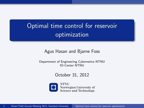
Optimal time control for reservoir optimization - NTNU

Optimal time control for reservoir
optimization
Agus Hasan and Bjarne Foss
Department of Engineering Cybernetics NTNU
IO-Center NTNU
October 31, 2012
1 Smart Field Annual Meeting 2012, Stanford University Optimal time control for reservoir optimization

IO-Center NTNU
IO-Center Collaborators
2 Smart Field Annual Meeting 2012, Stanford University Optimal time control for reservoir optimization

IO-Center NTNU
On going projects on production optimization
Short-term optimization
Production Optimization at Marlim Field (MINLP) → Vidar Gunnerud,
Petrobras.
Dual Control and MPC → Tor Aksel N. Heirung, Carnegie Mellon University.
Trustworthy Production Optimization → Bjarne Grimstad, BP.
Dynamics Production Optimization of Oil Fields at Urucu → Andres Codas
Duarte, Kongsberg.
Long-term optimization
Joining Well Placement and Well Control Decisions → Mathias Bellout,
Stanford University, IBM, Total.
Optimization of Late-life Shale-well Systems → Brage Rugstad Knudsen,
Carnegie Mellon University, Statoil, IBM.
Optimization and Control of Petroleum Reservoir (Voador and Troll Field) →
Agus Hasan, SINTEF, Statoil, Petrobras.
The Norne Benchmark → Richard Rwechungura, Statoil.
Long-term and Short-term optimization
Incorporating Long-term and Short-term Production Optimization →
Mansoureh Jesmani.
Completed projects
Gradient-based Methods for Production Optimization of Oil Reservoirs → Eka
Suwartadi, SINTEF.
Integrated Field Modeling and Optimization → Silvya Rahmawati, PERA AS.
3 Smart Field Annual Meeting 2012, Stanford University Optimal time control for reservoir optimization

IO-Center NTNU
SPE-Applied Technical Workshop 2013
Title : Integrated 4D Seismic & Production Data for Reservoir Management –
Application to Norne (Norway)
Place : Radisson BLU Royal Garden Hotel, Trondheim Norway
Time : 25th – 27th June 2013
Comparative case study
To utilize production and 4D seismic data from the full field Norne
Data, http://www.ipt.ntnu.no/~norne/, Package 2 Full Field Model 2013.
Exercise Description to include data integration
To utilize more seismic data
4 Smart Field Annual Meeting 2012, Stanford University Optimal time control for reservoir optimization

Outline
IO-Center NTNU
1 Introduction
2 Reservoir and well model
3 Gradient computation
4 Numerical example
5 Conclusions
5 Smart Field Annual Meeting 2012, Stanford University Optimal time control for reservoir optimization

CLRM
Introduction
6 Smart Field Annual Meeting 2012, Stanford University Optimal time control for reservoir optimization

Optimal control
Introduction
The optimal control problem may be stated in a canonical
form as follows
max
u
J(u) = ψ(x(T )) +
∫ T
0
L(x(t), u(t)) dt
Subject to ẋ(t) = A(x(t))x(t) + B(x(t))u(t)
x(0) = ¯x 0
u(t) ∈ U, ∀t ∈ [0, T ]
✁ ✁✕ U = {q ∈ R m : u min ≤ q ≤ u max }
✁
✁ ✁
Control Input
7 Smart Field Annual Meeting 2012, Stanford University Optimal time control for reservoir optimization

Optimal control
Introduction
The optimal control problem may be stated in a canonical
form as follows
max
u
J(u) = ψ(x(T )) +
∫ T
0
L(x(t), u(t)) dt
Subject to ẋ(t) = A(x(t))x(t) + B(x(t))u(t)
x(0) = ¯x 0
u(t) ∈ U, ∀t ∈ [0, T ]
✁ ✁✕ U = {q ∈ R m : u min ≤ q ≤ u max }
✁
✁ ✁
Control Input
7 Smart Field Annual Meeting 2012, Stanford University Optimal time control for reservoir optimization

Motivation
Introduction
u
✻
1
✻
❄
∂J
=? ∂u
✻
❄
0
✻
t 1
❄
t 2
✲
t
8 Smart Field Annual Meeting 2012, Stanford University Optimal time control for reservoir optimization

Motivation
Introduction
u
✻
1
✻
❄
∂J
=? ∂u
✻
❄
0
✻
t 1
❄
t 2
✲
t
8 Smart Field Annual Meeting 2012, Stanford University Optimal time control for reservoir optimization

Motivation
Introduction
u
✻
1
✻
❄
∂J
=? ∂u
✻
❄
0
✻
t 1
❄
t 2
✲
t
8 Smart Field Annual Meeting 2012, Stanford University Optimal time control for reservoir optimization

Motivation
Introduction
u
✻
1
0
✛✲
∂J
∂J
✛✲
∂t 1
=?
∂t 2
=?
t 1 t 2
✲
t
9 Smart Field Annual Meeting 2012, Stanford University Optimal time control for reservoir optimization

Motivation
Introduction
u
✻
1
0
✛✲
∂J
∂J
✛✲
∂t 1
=?
∂t 2
=?
t 1 t 2
✲
t
9 Smart Field Annual Meeting 2012, Stanford University Optimal time control for reservoir optimization

Motivation
Introduction
u
✻
1
0
✛✲
∂J
∂J
✛✲
∂t 1
=?
∂t 2
=?
t 1 t 2
✲
t
9 Smart Field Annual Meeting 2012, Stanford University Optimal time control for reservoir optimization

Reservoir and well model
State space representation
The standard black oil formulation for oil-water system may be written in
the following PDE
(
∂
∂t (φρ o[1 − s]) = ∇ · k k )
ro
ρ o ∇p + q o
µ o
(
∂
∂t (φρ ws) = ∇ · k k )
rw
ρ w ∇p + q w
µ w
Applying spatial discretization, the system may be written in the
following ODE
where
ẋ(t) = A(x(t))x(t) + B(x(t))u(t)
x(0) = ¯x 0
u(t) = [q 1 (t) q 2 (t) · · · q Nw (t)] ⊺ ∈ R Nw
10 Smart Field Annual Meeting 2012, Stanford University Optimal time control for reservoir optimization

Reservoir and well model
State space representation
The standard black oil formulation for oil-water system may be written in
the following PDE
(
∂
∂t (φρ o[1 − s]) = ∇ · k k )
ro
ρ o ∇p + q o
µ o
(
∂
∂t (φρ ws) = ∇ · k k )
rw
ρ w ∇p + q w
µ w
Applying spatial discretization, the system may be written in the
following ODE
where
ẋ(t) = A(x(t))x(t) + B(x(t))u(t)
x(0) = ¯x 0
u(t) = [q 1 (t) q 2 (t) · · · q Nw (t)] ⊺ ∈ R Nw
10 Smart Field Annual Meeting 2012, Stanford University Optimal time control for reservoir optimization

Well model
Reservoir and well model
The controls are given by the Peaceman model
q j (t) = α j (t)w j (s j )(p j R − pj bh (t)), j ∈ {N inj, N prod }
where α j (t) ∈ {[0, 1]} denotes the settings of the on-off valves of well j.
Linear relationship between q j and α j .
The term q j (t) in u may be replaced by α j (t) and the
corresponding entries in B are modified to include the term
w j (s j )(p j R − pj bh (t)).
11 Smart Field Annual Meeting 2012, Stanford University Optimal time control for reservoir optimization

Well model
Reservoir and well model
The controls are given by the Peaceman model
q j (t) = α j (t)w j (s j )(p j R − pj bh (t)), j ∈ {N inj, N prod }
where α j (t) ∈ {[0, 1]} denotes the settings of the on-off valves of well j.
Linear relationship between q j and α j .
The term q j (t) in u may be replaced by α j (t) and the
corresponding entries in B are modified to include the term
w j (s j )(p j R − pj bh (t)).
11 Smart Field Annual Meeting 2012, Stanford University Optimal time control for reservoir optimization

Well model
Reservoir and well model
The controls are given by the Peaceman model
q j (t) = α j (t)w j (s j )(p j R − pj bh (t)), j ∈ {N inj, N prod }
where α j (t) ∈ {[0, 1]} denotes the settings of the on-off valves of well j.
Linear relationship between q j and α j .
The term q j (t) in u may be replaced by α j (t) and the
corresponding entries in B are modified to include the term
w j (s j )(p j R − pj bh (t)).
11 Smart Field Annual Meeting 2012, Stanford University Optimal time control for reservoir optimization

Gradient Computation
Control parameterization
The idea is to parameterize the valve settings into a piecewise constant
function over the interval [0, T ] with switches at t j 1 , · · · , tj M j
as follows
M j
∑
α j (t) = γ j k χ [t j )(t), χ I(t) =
k ,tj k+1
k=0
{
1, t ∈ I
0, otherwise
The switching times t j k , k = 1, · · · , M j may be distinguished such that
0 = t j 0 < tj 1 < · · · < tj M j
< t j M j+1
= T
Let’s define the switching vectors as
v = [(t 1 1, · · · , t 1 M 1
) ⊺ , · · · , (t Nw
1 , · · · , t Nw
} {{ } } {{ }
v 1
v Nw
M Nw
) ⊺ ] ⊺
12 Smart Field Annual Meeting 2012, Stanford University Optimal time control for reservoir optimization

Gradient Computation
Gradient of the switching times
Theorem
For each j = 1, · · · , N w, the gradient of the functional J with respect to v j is given
by
⎡
H(x(t − 1 |v), u(t− 1 |v), λ(t− 1 |v))
⎤
−H(x(t + 1
∂J(v)
|v), u(t+ 1 |v), λ(t+ 1 |v))
∂v j =
.
⎢
⎣ H(x(t − M |v), u(t − j M |v), λ(t − j M |v)) ⎥
j ⎦
−H(x(t + M |v), u(t + j M |v), λ(t + j M |v))
j
where
H(x(t), u(t), λ(t)) = L(x(t), u(t)) + λ ⊺ (A(x(t))x(t) + B(x(t))u(t))
H(t + |v) = lim
τ→t + H(τ|v)
H(t − |v) = lim
τ→t − H(τ|v)
Computes the gradient w.r.t. switching times efficiently.
13 Smart Field Annual Meeting 2012, Stanford University Optimal time control for reservoir optimization

Gradient Computation
Applying heuristic search method - the halving
interval method
q
✻
1
✛
∂J
∂t s
< 0
0
t 0 t s t f
✲
t
14 Smart Field Annual Meeting 2012, Stanford University Optimal time control for reservoir optimization

Gradient Computation
Applying heuristic search method - the halving
interval method
q
✻
1
✛
∂J
∂t s
< 0
0
t 0 t s t f
✲
t
14 Smart Field Annual Meeting 2012, Stanford University Optimal time control for reservoir optimization

Gradient Computation
Applying heuristic search method - the halving
interval method
q
✻
1
✛
∂J
∂t s
< 0
0
t 0 t s t f
✲
t
14 Smart Field Annual Meeting 2012, Stanford University Optimal time control for reservoir optimization

Gradient Computation
Applying heuristic search method - the halving
interval method
q
✻
1
✛
∂J
∂t s
< 0
0
t 0 t s t f
✲
t
14 Smart Field Annual Meeting 2012, Stanford University Optimal time control for reservoir optimization

Gradient Computation
Applying heuristic search method - the halving
interval method
q
✻
1
0
t 0 t s t f
✲
t
15 Smart Field Annual Meeting 2012, Stanford University Optimal time control for reservoir optimization

Gradient Computation
Applying heuristic search method - the halving
interval method
q
✻
1
0
t 0 t s t f
✲
t
16 Smart Field Annual Meeting 2012, Stanford University Optimal time control for reservoir optimization

Gradient Computation
Applying heuristic search method - the halving
interval method
q
✻
1
0
∂J
∂t s
> 0 ✲
t 0 t s t f
✲
t
17 Smart Field Annual Meeting 2012, Stanford University Optimal time control for reservoir optimization

Gradient Computation
Applying heuristic search method - the halving
interval method
q
✻
1
0
∂J
∂t s
> 0 ✲
t 0 t s t f
✲
t
17 Smart Field Annual Meeting 2012, Stanford University Optimal time control for reservoir optimization

Gradient Computation
Applying heuristic search method - the halving
interval method
q
✻
1
0
∂J
∂t s
> 0 ✲
t 0 t s t f
✲
t
17 Smart Field Annual Meeting 2012, Stanford University Optimal time control for reservoir optimization

Gradient Computation
Applying heuristic search method - the halving
interval method
q
✻
1
0
t 0
t s
t f
✲
t
18 Smart Field Annual Meeting 2012, Stanford University Optimal time control for reservoir optimization

Gradient Computation
Applying heuristic search method - the halving
interval method
q
✻
1
0
t 0
t s
t f
✲
t
19 Smart Field Annual Meeting 2012, Stanford University Optimal time control for reservoir optimization

Gradient Computation
Applying heuristic search method - the halving
interval method
q
✻
1
✛
∂J
∂t s
< 0
0
t 0
t s
t f
✲
t
20 Smart Field Annual Meeting 2012, Stanford University Optimal time control for reservoir optimization

Gradient Computation
Applying heuristic search method - the halving
interval method
q
✻
1
✛
∂J
∂t s
< 0
0
t 0
t s
t f
✲
t
20 Smart Field Annual Meeting 2012, Stanford University Optimal time control for reservoir optimization

Gradient Computation
Applying heuristic search method - the halving
interval method
q
✻
1
✛
∂J
∂t s
< 0
0
t 0
t s
t f
✲
t
20 Smart Field Annual Meeting 2012, Stanford University Optimal time control for reservoir optimization

Gradient Computation
Applying heuristic search method - the halving
interval method
q
✻
1
0
t 0
t s
t f
✲
t
21 Smart Field Annual Meeting 2012, Stanford University Optimal time control for reservoir optimization

Gradient Computation
Applying heuristic search method - the halving
interval method
q
✻
1
0
t 0
t s
t f
✲
t
22 Smart Field Annual Meeting 2012, Stanford University Optimal time control for reservoir optimization

Simulation
Numerical example - Objective function
Suppose the aim is to
max
v
J NP V =
⎛
⎞
∫ T
⎝
∑
r o(t)qo j (t) −
∑
rw p qj w (t) +
∑
rw i qj w (t) ⎠
0
j∈N prod j∈N prod j∈N inj
1
× ( ) ct dt
1 + I
100
subject to the dynamical systems and control constraint.
23 Smart Field Annual Meeting 2012, Stanford University Optimal time control for reservoir optimization

Reservoir Model
Simulation
Figure: Grid and wells positions. Figure: Permeability distribution.
ref: K.-A. Lie, et.al., Open source MATLAB implementation of consistent
discretisations on complex grids, Comput. Geosci., Vol. 16, No. 2, pp. 297-322, 2012.
24 Smart Field Annual Meeting 2012, Stanford University Optimal time control for reservoir optimization

Reservoir Data
Simulation
Parameters Value Unit
qw, j j ∈ N inj 500 m 3 /day
rw i −63 USD/m 3
ro p 630 USD/m 3
rw p 63 USD/m 3
I 10 %
µ o 5 × 10 −3 Pa · s
µ w 1 × 10 −3 Pa · s
ρ o 859 kg/m 3
ρ w 1014 kg/m 3
Table: Simulation parameters.
25 Smart Field Annual Meeting 2012, Stanford University Optimal time control for reservoir optimization

Simulation
Optimization settings
The injection rates are set constant for both injection
wells at 500 m 3 /day.
The control variables are the switching times in both
horizontal production wells, namely t 1 1, t 1 2, t 2 1, and t 2 2.
The optimization is run for 512 days. The method is
compared with Reactive control strategy with water cut
treshold is 0.82.
26 Smart Field Annual Meeting 2012, Stanford University Optimal time control for reservoir optimization

Simulation
Optimal well settings
27 Smart Field Annual Meeting 2012, Stanford University Optimal time control for reservoir optimization

Objective function
Simulation
28 Smart Field Annual Meeting 2012, Stanford University Optimal time control for reservoir optimization

Conclusions
Conclusions
A novel optimal switching times method for an oil
reservoir, given the optimal settings of the wells to be
bang-bang controls, has been presented.
The bang-bang control has a major practical advantage
since it can be implemented with simple on-off valves.
The optimal control settings are obtained based on
gradient calculation using the adjoint method combined
with the halving interval method.
The gradient calculation is supported by a formal proof.
An example of a realistic reservoir show that the proposed
method can be used to increase oil revenue significantly.
Submitted to European Control Conference 2013.
29 Smart Field Annual Meeting 2012, Stanford University Optimal time control for reservoir optimization

Conclusions
Conclusions
A novel optimal switching times method for an oil
reservoir, given the optimal settings of the wells to be
bang-bang controls, has been presented.
The bang-bang control has a major practical advantage
since it can be implemented with simple on-off valves.
The optimal control settings are obtained based on
gradient calculation using the adjoint method combined
with the halving interval method.
The gradient calculation is supported by a formal proof.
An example of a realistic reservoir show that the proposed
method can be used to increase oil revenue significantly.
Submitted to European Control Conference 2013.
29 Smart Field Annual Meeting 2012, Stanford University Optimal time control for reservoir optimization

END
Thanks you.
Questions?
30 Smart Field Annual Meeting 2012, Stanford University Optimal time control for reservoir optimization