ON OPTIMIZING NONLINEAR ADAPTIVE CONTROL ... - NTNU
ON OPTIMIZING NONLINEAR ADAPTIVE CONTROL ... - NTNU
ON OPTIMIZING NONLINEAR ADAPTIVE CONTROL ... - NTNU

Create successful ePaper yourself
Turn your PDF publications into a flip-book with our unique Google optimized e-Paper software.
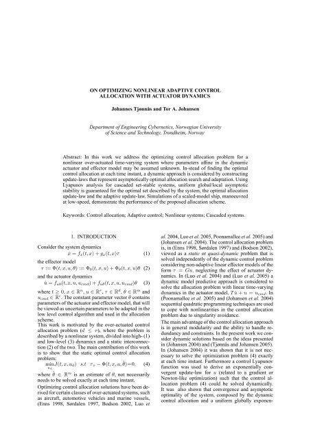
<strong>ON</strong> <strong>OPTIMIZING</strong> N<strong>ON</strong>LINEAR <strong>ADAPTIVE</strong> C<strong>ON</strong>TROL<br />
ALLOCATI<strong>ON</strong> WITH ACTUATOR DYNAMICS<br />
Johannes Tjønnås and Tor A. Johansen<br />
Department of Engineering Cybernetics, Norwegian University<br />
of Science and Technology, Trondheim, Norway<br />
Abstract: In this work we address the optimizing control allocation problem for a<br />
nonlinear over-actuated time-varying system where parameters afne in the dynamic<br />
actuator and effector model may be assumed unknown. In-stead of nding the optimal<br />
control allocation at each time instant, a dynamic approach is considered by constructing<br />
update-laws that represent asymptotically optimal allocation search and adaptation. Using<br />
Lyapunov analysis for cascaded set-stable systems, uniform global/local asymptotic<br />
stability is guaranteed for the optimal set described by the system, the optimal allocation<br />
update-law and the adaptive update-law. Simulations of a scaled-model ship, manoeuvred<br />
at low-speed, demonstrate the performance of the proposed allocation scheme.<br />
Keywords: Control allocation; Adaptive control; Nonlinear systems; Cascaded systems.<br />
1. INTRODUCTI<strong>ON</strong><br />
Consider the system dynamics<br />
_x = f x (t; x) + g x (t; x) (1)<br />
the effector model<br />
:= (t; x; u; ) := 0 (t; x; u) + (t; x; u) (2)<br />
and the actuator dynamics<br />
_u = f u0 (t; x; u; u cmd ) + f u (t; x; u; u cmd ) (3)<br />
where t 0; x 2 R n ; u 2 R r ; 2 R d ; 2 R m and<br />
u cmd 2 R c : The constant parameter vector contains<br />
parameters of the actuator and effector model, that will<br />
be viewed as uncertain parameters to be adapted in the<br />
low level control algorithm and used in the allocation<br />
scheme.<br />
This work is motivated by the over-actuated control<br />
allocation problem (d r), where the problem is<br />
described by a nonlinear system, divided into high- (1)<br />
and low-level (3) dynamics and a static interconnection<br />
(2) of the two. The main contribution of this work<br />
is to show that the static optimal control allocation<br />
problem:<br />
minJ(t; x; u d ) s:t x (t; x; u; ^)=0; (4)<br />
u d<br />
where ^ 2 R m is an estimate of , not necessarily<br />
needs to be solved exactly at each time instant.<br />
Optimizing control allocation solutions have been derived<br />
for certain classes of over-actuated systems, such<br />
as aircraft, automotive vehicles and marine vessels,<br />
(Enns 1998, Sørdalen 1997, Bodson 2002, Luo et<br />
al. 2004, Luo et al. 2005, Poonamallee et al. 2005) and<br />
(Johansen et al. 2004). The control allocation problem<br />
is, in (Enns 1998, Sørdalen 1997) and (Bodson 2002),<br />
viewed as a static or quasi-dynamic problem that is<br />
solved independently of the dynamic control problem<br />
considering non-adaptive linear effector models of the<br />
form = Gu; neglecting the effect of actuator dynamics.<br />
In (Luo et al. 2004) and (Luo et al. 2005) a<br />
dynamic model predictive approach is considered to<br />
solve the allocation problem with linear time-varying<br />
dynamics in the actuator model, T _u + u = u cmd . In<br />
(Poonamallee et al. 2005) and (Johansen et al. 2004)<br />
sequential quadratic programming techniques are used<br />
to cope with nonlinearities in the control allocation<br />
problem due to singularity avoidance.<br />
The main advantage of the control allocation approach<br />
is in general modularity and the ability to handle redundancy<br />
and constraints. In the present work we consider<br />
dynamic solutions based on the ideas presented<br />
in (Johansen 2004) and (Tjønnås and Johansen 2005).<br />
In (Johansen 2004) it was shown that it is not necessary<br />
to solve the optimization problem (4) exactly<br />
at each time instant. Furthermore a control Lyapunov<br />
function was used to derive an exponentially convergent<br />
update-law for u (related to a gradient or<br />
Newton-like optimization) such that the control allocation<br />
problem (4) could be solved dynamically.<br />
It was also shown that convergence and asymptotic<br />
optimality of the system, composed by the dynamic<br />
control allocation and a uniform globally exponen-
tially stable trajectory-tracking controller, guarantees<br />
uniform boundedness and uniform global exponential<br />
convergence to the optimal solution of the system.<br />
In (Tjønnås and Johansen 2005) the results from<br />
(Johansen 2004) were extended by allowing uncertain<br />
parameters, associated with an adaptive law, in the<br />
effector model, and by applying set-stability analysis<br />
in order to also conclude asymptotic stability of the<br />
optimal solution.<br />
In what follows we will extend the ideas from<br />
(Tjønnås and Johansen 2005) by introducing dynamics<br />
in the actuator model, and nally we present an<br />
example of this control allocation approach, where<br />
dynamic positioning (DP) of a model ship in different/changing<br />
weather conditions, controlled by<br />
thrusters experiencing thrust losses, is considered.<br />
Whenever referring to the notion of set-stability, the<br />
set has the property of being nonempty, and we strictly<br />
follow the denitions given in (Tjønnås et al. 2006)<br />
motivated by (Teel et al. 2002) and (Lin et al. 1996).<br />
2. <strong>ADAPTIVE</strong> C<strong>ON</strong>TROL ALLOCATI<strong>ON</strong> WITH<br />
ACTUATOR DYNAMICS<br />
Our results rests on the following assumptions:<br />
Assumption 1. (Plant)<br />
a) The states of (1) and (3) are know for all t > t 0 :<br />
b) There exist a continuous function G f : R 0 !<br />
R >0 and a constant B g ; such that jf x (t; x)j <br />
G f (jxj) and jg x (t; x)j B g for all t and x. Moreover<br />
f x is locally Lipschitz in t and x.<br />
c) There exist a continuous function & @gx : R 0 !<br />
R 0 such that for all t and x; g x is differentiable<br />
and @gx<br />
@t<br />
+ @gx<br />
@x<br />
& @gx (jxj).<br />
d) The function from the static mapping (2) is twice<br />
differentiable and there exist a continuous function<br />
G : R 0 ! R 0 ; such that j j + j 0 j <br />
<br />
G x T ; u T <br />
T for all t; x; and u. Further there<br />
exist a continuous function & @ (jxj) @ <br />
@t +<br />
@ 0 <br />
@t + @ <br />
@x + @ 0 <br />
@x + @ <br />
@u + @ 0 <br />
@u where<br />
& @ : R 0 ! R 0 :<br />
e) There exists constants % 2 > % 1 > 0, such that<br />
8t, x, u and <br />
% 1 I @<br />
@u (t; x; u; ) @<br />
@u (t; x; u; ) T<br />
% 2 I: (5)<br />
Assumption 2. (High/low level control algorithms)<br />
a) There exists a high level control x := k x (t; x);<br />
where jk x (t; x)j & k (jxj) and & k : R 0 7! R 0 is<br />
a continuous function, that render the equilibrium<br />
of (1) UGAS for = x . The function k x is<br />
differentiable, @k x <br />
@t + @k x <br />
@x &@kx (jxj); where<br />
& @kx : R 0 7! R 0 is continuous.<br />
b) There exists a low-level control<br />
u cmd := k u (t; x; u; u d ; _u d ; ^) that makes the equilibrium<br />
of<br />
_~u = f ~u (t; x; ~u; u d ; ^; ); (6)<br />
where ~u := u u d and f ~u (t; x; ~u; u d ; ^; ) :=<br />
f u0 (t; x; u; u cmd )+f u (t; x; u; u cmd )<br />
UGAS if ^ = ; and if x; u d ; _u d exist for all t > 0.<br />
Furthermore k u (t; x; u; u d ; _u d ; ^) & u (ju u d j);<br />
where & u : R 0 7! R 0 ; is a continuous differentiable<br />
function. Moreover @k u <br />
@t + @k u <br />
@x +<br />
f d (t; x; ~u; u d ; ^),<br />
@k u <br />
@u +<br />
@k u <br />
@u d<br />
+<br />
@k u <br />
@ _u d<br />
&@ku (ju<br />
: R 0 7! R 0 is continuous.<br />
& @ku<br />
u d j); where<br />
Remark 1. From assumption 2a) there exist a Lyapunov<br />
function V x : R 0 R n 7! R 0 that satisfy:<br />
x1 (jxj) V x (t; x) x2 (jxj) (7)<br />
@V x<br />
@t + @V x<br />
@x f(t; x) x3(jxj) (8)<br />
@V x<br />
@x x4(jxj); (9)<br />
where x1 ; x2 ; x3 ; x4 2 K 1 ; for the system<br />
_x = f(t; x) := f x (t; x) + g x (t; x)k x (t; x); where<br />
g(t; x) := g x (t; x): If x(t), u d (t), _u d (t); and ^(t) =<br />
(t) exist for all t then there also exist a function<br />
V ~u : R 0 R n ! R 0 and K 1 functions ~u1 ; ~u2 ;<br />
~u3 such that<br />
~u1 (j~uj) V ~u (t; ~u) ~u2 (j~uj) (10)<br />
@V ~u<br />
@t + @V ~u<br />
@~u f ~u(t;x(t); ~u;u d (t);^(t);(t)) ~u3 (j~uj): (11)<br />
We will not discuss the details in these assumptions,<br />
but they are sufcient in order to guarantee existence<br />
of solutions and validity of the update-laws that we<br />
propose in this paper.<br />
By assumption 2 a) we may consider a Series Parallel<br />
estimation model:<br />
_^u=A^u (u ^u) +f u0 (t;x;u;u cmd ) +f u (t;x;u;u cmd )^;<br />
(12)<br />
where ( A^u ) is Hurwitz. This estimation model is<br />
used in a Lyapunov based indirect scheme in order to<br />
estimate the unknown but bounded parameter vector<br />
: For analytical purpose we use the error estimate:<br />
_ = A^u + f u (t; x; u; u cmd ) ~ (13)<br />
where := u ^u and ~ := ^:<br />
The adaptive structure of the algorithm, that we will<br />
present, is based on dening the adaptive law at the<br />
low level, incorporating the low level control algorithm<br />
and passing these parameter estimates to the<br />
control allocation algorithm. Generally we consider an<br />
adaptive control allocation approach of four modular<br />
steps where the contribution of this paper is on step<br />
three and four and the interconnection of these steps,<br />
see also Figure 1.<br />
(1) The high-level control algorithm. The virtual<br />
control is treated as an available input to the<br />
system (1), and a virtual control law x is designed<br />
such that the origin of (1) is UGAS when<br />
= x .<br />
(2) The low-level control algorithm. The actuator<br />
dynamic is controlled by the actuators through<br />
an control law u cmd ; such that for any smooth<br />
reference u d ; u tracks u d asymptotically.<br />
(3) The control allocation algorithm (Connecting<br />
the high and low level control). Based<br />
on the minimization problem (4) where J is a<br />
cost function that incorporates objectives such as<br />
minimum power consumption and actuator constraints<br />
(implemented as barrier functions), the<br />
Lagrangian function<br />
L^(t; x; u d ; ~u; ) := J(t; x; u d )<br />
+ (k x (t; x) (t; x; u d + ~u; ^)) T (14)
Fig. 1. Adaptive control allocation design philosophy<br />
is introduced, and update laws for the effector<br />
reference u d and the Lagrangian parameter are<br />
then dened such that u d and converges to a set<br />
dened by the time-varying optimality condition.<br />
(4) The adaptive algorithm. In order to cope with<br />
an possibly unknown parameter vector in the<br />
effector and actuator models, an adaptive law<br />
is dened. The parameter estimate is used in<br />
the control allocation scheme and a certainty<br />
equivalent adaptive optimal control allocation<br />
algorithm can be dened.<br />
Based on Assumption 1 and 2 together with the following<br />
assumption;<br />
Assumption 3. (Optimal control allocation)<br />
a) The cost function J : R t0 R nr ! R is<br />
twice differentiable and satises: J(t; x; u d ) ! 1<br />
as ju d j ! 1. Further there exists a continuous<br />
function & @2 J : R 0 ! R 0 such that @2 J <br />
@t@u d<br />
+<br />
@2 J <br />
@x@u d<br />
&@ 2 J( x T ; u T d ; T ) 8 t; x; u d and :<br />
b) There exists constants k 2 > k 1 > 0, such that 8 t;<br />
x; ~u; ^ and (u T d ; T ) T =2 O ud ; where<br />
(<br />
! )<br />
O ud (t; x) := u T d; T 2 R r+d @L<br />
<br />
T^ ; @LT^ =0 ;<br />
@u d @<br />
then<br />
k 1 I @2 L^<br />
@u 2 (t; x; u d ; ~u; ; ^) k 2 I: (15)<br />
d<br />
If (u T d ; T ) T 2 O ud ; the lower bound is replaced<br />
by @2 L^<br />
@u 2 d<br />
0.<br />
we formulate our main problem:<br />
Problem: Dene update-laws for u d , ^ and such that<br />
the stability of the closed loop:<br />
_x = f(t; x)<br />
1 :<br />
(16)<br />
+g(t; x) ((t; x; u d + ~u; ) k x (t; x))<br />
8<br />
_~u = f ~u (t; x; ~u; u d ; ^; )<br />
>< _u d = f d (t; x; ~u; u d ; ^)<br />
2 : _ = f (t; x; u d ; ^)<br />
_ = A + f u (t; x; u; u cmd )<br />
>:<br />
~ (17)<br />
<br />
_~ = f^(t; x; u cmd ; ~u; u d ; ^);<br />
from (1), (2), (3), (6) and (13), is conserved and u d (t)<br />
converges to an optimal solution with respect to the<br />
minimization problem (4).<br />
Note that system (16)-(17) takes the form of a cascade<br />
as long as x(t) exists, and is viewed as a time-varying<br />
input to 2 ; for all t > 0: We deal with the problem<br />
formulated by: i) dening a Lyapunov like function,<br />
V ud ~u ~ ; for system 2 and dening explicit updatelaws<br />
for u d , and ~ such that V _ ud ~u ~ 0: ii) Further,<br />
we prove boundedness of the closed-loop system,<br />
1 and 2 ; and use the cascade lemma (Tjønnås et<br />
al. 2006) to prove convergence and stability.<br />
Based on the Lyapunov like function candidate<br />
V ud ~u ~ (t; x; u d; ; ~u; ) := V ~u (t; ~u) + 1 2 T <br />
!<br />
+ 1 @L T^ @L^<br />
+ @LT^ @L^<br />
+ 1 2 @u d @u d @ @ 2 ~ T ~<br />
~ ; (18)<br />
we suggest the following control allocation algorithm:<br />
<br />
! _u T d; _ T T T<br />
=<br />
@L^ H^<br />
; @L^<br />
T<br />
T<br />
u<br />
@u d @<br />
ff^<br />
(19)<br />
<br />
_^ T = 1 @V~u<br />
~ @~u + T f u (t; x; u; u cmd );<br />
!<br />
@L T^ + 1 @ 2 L^<br />
+ @LT^ @ 2 L^<br />
f<br />
~<br />
u (t; x; u; u cmd )<br />
@u d @~u@u d @ @~u@<br />
@L T^ + 1 @ 2 L^<br />
~<br />
@<br />
@L T^ + 1 @ 2 L^<br />
~<br />
@x@ g(t; x) (t; x; u)<br />
g(t; x) (t; x; u) (20)<br />
@u d @x@u d<br />
0<br />
1<br />
@ 2 L^<br />
@u 2 d<br />
@ 2 L^<br />
@ 2 L^<br />
where H^<br />
: = B @@u d C<br />
@<br />
A ; is a possibly<br />
0<br />
@u d @<br />
time-varying symmetric positive denite weighting<br />
matrix, and u ff^<br />
:= H 1<br />
^ u F is a feed-forward like<br />
term, where: ! ; @2 T T<br />
!<br />
L^<br />
+ @2 T<br />
L^<br />
; @2 T T<br />
L^<br />
f(t; x)<br />
@t@ @x@u d @x@<br />
u F := @2 T<br />
L^<br />
@t@u d<br />
+ @2 L T^ ; @2 L T^<br />
@x@u d @x@<br />
+ @2 L T^<br />
@~u@u d<br />
; @2 L T^<br />
@~u@<br />
! T<br />
g(t; x)(k x (t; x) (t; x; u d +~u; ^))<br />
! T<br />
f ~u (t; x; ~u; u d ; ^; ^)+ @2 L T^<br />
!<br />
; @2 L T_^:<br />
T^<br />
@^@u d @^@<br />
if det(H) 6= 0;and u ff^<br />
:= 0 if det(H) = 0: Hence<br />
the time derivative of V ud ~u ~ along the trajectories of<br />
(1), (3), (6), (19) and (20) is:<br />
_V ud ~u ~ = T A ~u3 (j~uj)<br />
@L<br />
T<br />
; @L T @L<br />
T<br />
H^<br />
H^<br />
; @L T T : (21)<br />
@u d @ @u d @
In order to prove a global result we need to make an<br />
additional assumption on (t; x; u): The assumption<br />
is based on the following lemma<br />
Lemma 1. By Assumption 1 and (Mazenc and Praly<br />
1996)'s lemma B.1 there exists continuous functions<br />
& x ; & xu , & u : R 0 ! R 0 ; such that<br />
j (t; x; u)j & x (jxj)& xu (jxj)<br />
!<br />
zud <br />
+ & x (jxj)& u ~u ~<br />
<br />
Oud<br />
~u ~ <br />
where<br />
O ud ~ (t;x): =O u d (t;x)<br />
<br />
n~u T ; T ; ~ T <br />
2R 2r+m <br />
~u T ; T ; ~ T o<br />
=0<br />
and z ud ~ := u T d ; T ; ~u T ; T ; ~ T T<br />
:<br />
Assumption 2. (Continued)<br />
c) There exists a K 1 function k : R 0 ! R 0 ;<br />
such that<br />
1<br />
k (jxj) x3(jxj) x4 (jxj)& x max (jxj) , (22)<br />
where & x max (jxj):=max(1; & x (jxj); & x (jxj)& xu (jxj)):<br />
Proposition 1. If the assumptions 1, 2 and 3 are<br />
satised, then the solution of the closed-loop (16)-<br />
(17) is bounded with respect to a set O xud ~ (t) :=<br />
O ud ~ (t; 0)fx 2 Rn jx = 0g: Furthermore O xud ~ (t)<br />
is UGS with respect to the system (16)-(17): If in<br />
addition f u (t) := f u (t; x(t); u(t); u cmd (t)) is Persistently<br />
Exited (PE), then O xud ~ (t) is UGAS with<br />
respect to system (16)-(17).<br />
PROOF. Sketch: The main steps of this proof is to<br />
prove: i) that (18) is a Lyapunov function, when x(t) is<br />
assumed to be a signal that exists for all t; with respect<br />
to O ud ~ ; ii) boundedness and stability of the closed<br />
loop system and iii) attractivity when f u (t) is PE.<br />
i) By similar arguments as in the proof of Proposition<br />
1 (i) in (Tjønnås and Johansen 2005) it can be shown<br />
that O ud ~ is a closed forward invariant set with respect<br />
to 2 : Further it can be shown that system 2<br />
<br />
is nite escape time detectable through z ud ~<br />
<br />
Oud<br />
~ <br />
and by using theorem 2.4.7 in (Abrahamson et al.<br />
1988) and a similar approach as presented in the<br />
proof of Claim 3 in (Tjønnås and Johansen 2005),<br />
it can be shown that V ud ~u ~ (t; x; u d; ; ~u; ) is radially<br />
unbounded Lyapunov function with respect to<br />
<br />
z ud ~ :<br />
<br />
Oud<br />
~ <br />
ii) By dening v(t; x) := V x (t; x); it can be shown<br />
from Assumption 2 c) and V ud ~u ~ that jx(t)j <br />
M(r): Then by applying the cascade lemma from<br />
(Tjønnås et al. 2006) the UGS result is proved.<br />
iii) By following ideas from the proof of the main<br />
result in (Tjønnås and Johansen 2005), the integral of<br />
~ T ~ can be shown to be bounded by the PE assumption,<br />
furthermore from this bound the uniform attractivity<br />
of the set O xud ~ can be shown by contradiction.<br />
<br />
Proposition 1 implies that the time-varying rst order<br />
optimal set O xud ~ (t) is uniformly stable, and in<br />
addition uniformly attractive if a PE assumption is<br />
satised. Thus adaptive optimal control allocation is<br />
achieved asymptotically for the closed loop system<br />
(16)-(17).<br />
Remark 2. If the unknown parameter vector in the<br />
effector model (2), is not the same as in the unknown<br />
parameter vector in the actuator dynamic (3), the low<br />
level adaptive control law dened in this paper may be<br />
combined with the adaptive law presented in (Tjønnås<br />
and Johansen 2005). The analysis of this case will be<br />
considered in future work.<br />
3. EXAMPLE<br />
In this section simulation results of an over-actuated<br />
scaled-model ship, manoeuvred at low-speed, is presented.<br />
The scale model-ship is moved while experiencing<br />
static disturbances, caused by wind and current,<br />
and propellers trust losses. The propeller losses<br />
can be due to: Axial Water Inow, Cross Coupling<br />
Drag, Thruster-Hull and Thruster-Thruster Interaction<br />
(see (Sørensen et al. 1997) and (Fossen and<br />
Blanke 2000) for details). But in this example we limit<br />
our study to thruster loss caused by Thruster-Hull interaction.<br />
A 3DOF horizontal plane model described<br />
by:<br />
_ e = R( p )<br />
_ = M 1 D + M 1 ( + b) (23)<br />
= (u; );<br />
is considered, where e := (x e ; y e ; e ) T := (x p<br />
x d ; y p y d ; p d ) T is the north and east positions<br />
and compass heading deviations. Subscript p and d denotes<br />
the actual and desired states. := ( x ; y ; r) T<br />
is the body-xed velocities in surge, sway and yaw,<br />
is the generalized force vector, b := (b 1 ; b 2 ; b 3 ) T is<br />
a static disturbance and R( p ) is the rotation matrix<br />
function between the body xed and the earth xed coordinate<br />
frame. The example we present here is based<br />
on (Lindegaard and Fossen 2003), and is also studied<br />
in (Johansen 2004) and (Tjønnås and Johansen 2005).<br />
In the considered model there are ve force producing<br />
devices; the two main propellers aft of the hull, in<br />
conjunction with two rudders, and one tunnel thruster<br />
going through the hull of the vessel. ! i denotes the<br />
propeller angular velocity and i denotes the rudder<br />
deection. i = 1; 2 denotes the aft actuators, while<br />
i = 3 denotes the tunnel thruster. Eq. (23) can be<br />
rewritten in the form of (1) and (2) by:<br />
x := ( e ; ) T ; := ( 1 ; 2 ; 3 ) T ; :=( 1 ; 2 ; 3 ) T<br />
<br />
u:=(! 1 ; ! 2 ; ! 3 ; 1 ; 2 ) T R(<br />
; f x :=<br />
e + d )<br />
;<br />
(; u; ):=G u (u)<br />
T 1 ( x ; ! 1 ; 1 )<br />
T 2 ( x ; ! 2 ; 2 )<br />
T 3 ( x ; y ; ! 3 ; 3 )<br />
M 1 D + M 1 b<br />
! 0<br />
; g x :=<br />
M 1 ;<br />
!<br />
(1 D 1 ) (1 D 2 ) 0<br />
G u (u) := L 1 L 2 1<br />
31 32 l 3;x<br />
3i (u) := l i;y (1 D i (u) + l i;x L i (u)):<br />
The truster forces are given by:
T i ( x ; ! i ; i ) := T ni (! i ) i (! i ; x ) i (24)<br />
<br />
kT<br />
T ni (! i ) := pi ! 2 i ! i 0<br />
k T ni j! i j ! i ! i < 0 ;<br />
q<br />
i (! i ; x ) = ! i x ; 3 (! 3 ) := ( 2 x + 2 y) j! 3 j ! 3<br />
<br />
kT<br />
i =<br />
i (1 w) x 0<br />
x < 0 ; 3 := k T 3<br />
k T i<br />
where 0 < w < 1 is the wake fraction number,<br />
i (! i ; x ) i is the thrust loss due to changes in the<br />
advance speed, a = (1 w) x ; and the unknown<br />
parameters i represents the thruster loss factors dependent<br />
on whether the hull invokes on the inow of<br />
the propeller or not. The rudder lift and drag forces are<br />
projected through:<br />
(1+kLni !<br />
L i (u):=<br />
i )(k L1i +k L2i j i j) i ; ! i 0<br />
0 ; ! i < 0 ;<br />
<br />
(1+kDni !<br />
D i (u):=<br />
i )(k D1i j i j+k D2i 2 i ) ; ! i 0<br />
0 ; ! i < 0 :<br />
Furthermore it is clear from (24) that (; u; ) =<br />
G u (u)Q(u) + G u (u)(!; x ); where (!; x ) :=<br />
diag( 1 ; 2 ; 3 ) and Q(u) represents the nominal<br />
propeller thrust.<br />
The actuator error dynamic for each propeller is based<br />
on the propeller model presented in (Pivano et al.<br />
2007) and given by<br />
T ni<br />
J mi<br />
_~! i = k fi (~! i + ! di ) (~! i + ! di )<br />
a T<br />
+ i(! i ; x ) i<br />
a T<br />
+ u cmdi J mi _! di (25)<br />
where ~! i := (! i ! id ); J m is the shaft moment of<br />
inertia, k f is a positive coefcient related to the viscous<br />
friction, a T is a positive model constant (Pivano<br />
et al. 2006) and u cmd is the motor torque. By the<br />
quadratic Lyapunov function V ~!i := ~!2 i<br />
2<br />
it is easy to<br />
see that the control law<br />
<br />
u cmdi := K !p ~! i (! i ; x )^ i<br />
i + J mi _! di<br />
a T<br />
+ T ni(! di )<br />
+ k fi ! di : (26)<br />
a T<br />
makes the origin of (25) UGES when ^ i = i . The<br />
error dynmaics of the rudder is given by:<br />
m i <br />
_~ = ai ~ + di + b i u cmdi m i di _ (27)<br />
where ~ := i di , a i (t) is a known scalar function,<br />
b i is a known scalar parameter bounded away from<br />
zero, and the controller <br />
b i u cmdi := K <br />
~ ai (t) ~ + di + m i di _ (28)<br />
makes the origin of (27) UGES. The parameters for<br />
the actuator model and controllers are: a T = 1;<br />
J mi = 10 2 ; kf i = 10 4 ; a i = 10 4 ; b i = 10 5 ,<br />
m i = 10 2 ; K !p = 5 10 3 and K = 10 3<br />
A virtual controller c that stabilizes the system (23)<br />
uniformly, globally and exponentially; for some physically<br />
limited yaw rate, is proposed in (Lindegaard and<br />
Fossen 2003) and given by<br />
x := K i R T ( p ) K p R T ( p ) e K d ; (29)<br />
where (23) is augmented with the integral action state,<br />
_ = e :<br />
The cost function designed for the optimization problem,<br />
(4), is:<br />
η e1 [m]<br />
η e2 [m]<br />
η e3 [deg]<br />
1.5<br />
0.5<br />
0.5<br />
0.5<br />
1<br />
0<br />
1.5<br />
1<br />
0.5<br />
0.05<br />
0<br />
0.15<br />
0.1<br />
0.05<br />
0<br />
0 100 200 300 400 500 600<br />
0 100 200 300 400 500 600<br />
0 100 200 300 400 500 600<br />
t [s]<br />
Fig. 2. Desired (dashed) and actual ship positions<br />
(solid).<br />
ω 1 [Hz]<br />
ω 2 [Hz]<br />
ω 3 [Hz]<br />
5<br />
10<br />
15<br />
10<br />
5<br />
0<br />
20<br />
10<br />
10<br />
0<br />
20<br />
10<br />
0<br />
0 100 200 300 400 500 600<br />
0 100 200 300 400 500 600<br />
0 100 200 300 400 500 600<br />
t [s]<br />
Fig. 3. Actual propeller velocities<br />
3X<br />
2X 3X<br />
J(u):= k i j! i j ! 2 i + q i 2 i & lg( ! i + 18)<br />
i=1<br />
3X<br />
& lg(! i +18)<br />
i=1<br />
i=1<br />
i=1<br />
2X<br />
& lg( i +35)<br />
i=1<br />
2X<br />
& lg( i +35);<br />
i=1<br />
w = 0:05; k 1 = k 2 = 0:01; k 3 =0:02; q 1 = q 2 =500:<br />
The gain matrices are chosen as follows: A^u :=<br />
2I 55 ; ~ := 10 3 ; := diag(10 3 ; 10 3 ; 3) and<br />
<br />
:= H T^W 1<br />
H^<br />
+ "I<br />
where<br />
W := diag (1; 1; 1; 1; 1; 0:9; 0:9; 0:7) and " := 10 9 .<br />
The weighting matrix W is dened such that the<br />
<br />
deviation of @L^<br />
@<br />
= k(t; x) (t; x; u; ^)<br />
from<br />
zero is penalized more then the deviation of @L^<br />
@u<br />
<br />
from zero in the search direction.<br />
The static disturbance vector is b := 0:05(1; 1; 1) T ,<br />
and the thruster loss vector is given in Figure 6.<br />
The simulation results are presented in the Figures<br />
2-7. The control objective is satised and the commanded<br />
virtual controls are tracked closely by the<br />
forces generated by the adaptive control allocation<br />
law: see Figure 5. Note that there are some deviations<br />
since ! saturates at ca. 220s and 420s: Also note<br />
that the parameter estimates only converge to the true<br />
values when the ship is moving and the thrust loss is<br />
not zero. The simulations are carried out in a discrete<br />
MATLAB environment with a sampling rate of 20Hz:
δ 1 [deg]<br />
10<br />
5<br />
0<br />
5<br />
10<br />
0 100 200 300 400 500 600<br />
20<br />
15<br />
loss 1 [N]<br />
loss 2 [N]<br />
0.2<br />
0.1<br />
0<br />
0.1<br />
0.2<br />
0 100 200 300 400 500 600<br />
0.4<br />
0.2<br />
0<br />
0.2<br />
0.4<br />
0 100 200 300 400 500 600<br />
δ 2 [deg]<br />
10<br />
5<br />
10<br />
15<br />
5<br />
0<br />
0 100 200 300 400 500 600<br />
t [s]<br />
Fig. 4. Actual rudder deection<br />
τ 1 [N]<br />
τ 2 [N]<br />
τ 3 [Nm]<br />
0.05<br />
0.05<br />
0.1<br />
0.15<br />
0.2<br />
0.4<br />
0<br />
0.4<br />
0.2<br />
0.02<br />
0.04<br />
0.06<br />
0.08<br />
0<br />
0<br />
0 100 200 300 400 500 600<br />
0 100 200 300 400 500 600<br />
0 100 200 300 400 500 600<br />
t [s]<br />
Fig. 5. The virtual control (dashed) and actual (solid)<br />
forces generated by the actuators<br />
θ 1<br />
θ 2<br />
θ 3<br />
0.4<br />
0.2<br />
0.4<br />
0.2<br />
1.5<br />
0.5<br />
0<br />
0 100 200 300 400 500<br />
0<br />
0 100 200 300 400 500<br />
1<br />
x 10<br />
3<br />
0<br />
0 100 200 300 400 500<br />
t [s]<br />
Fig. 6. Actual (dashed) and estimated (solid) loss<br />
parameters<br />
4. ACKNOWLEDGEMENT<br />
The authors are grateful to Luca Pivano at <strong>NTNU</strong>,<br />
for insightful comments. This work is sponsored by<br />
the Research Council of Norway through the Strategic<br />
University Programme on Computational Methods in<br />
Nonlinear Motion Control<br />
REFERENCES<br />
Abrahamson, H., J. E. Marsden and T. Ratiu (1988). Manifolds,<br />
Tensor Analysis and applications. 2'nd ed.. Springer-Verlag.<br />
Bodson, M. (2002). Evaluation of optimization methods for control<br />
allocation. J. Guidance, Control and Dynamics 25, 703–711.<br />
loss 3 [Nm]<br />
0.02<br />
0.01<br />
0.01<br />
0<br />
0 100 200 300 400 500 600<br />
t [s]<br />
Fig. 7. Actual thrust loss<br />
Enns, D. (1998). Control allocation approaches. In: Proc. AIAA<br />
Guidance, Navigation and Control Conference and Exhibit,<br />
Boston MA. pp. 98–108.<br />
Fossen, T. I. and M. Blanke (2000). Nonlinear output feedback<br />
control of underwater vehicle propellers using feedback form<br />
estimated axial ow velocity. IEEE JOURNAL OF OCEANIC<br />
ENGINEERING 25(2), 241–255.<br />
Johansen, T. A. (2004). Optimizing nonlinear control allocation.<br />
Proc. IEEE Conf. Decision and Control. Bahamas pp. 3435–<br />
3440.<br />
Johansen, T. A., T. I. Fossen and Svein P. Berge (2004). Constrained<br />
nonlinear control allocation with singularity avoidance using<br />
sequential quadratic programming. IEEE Trans. Control Systems<br />
Technology 12, 211–216.<br />
Lin, Y., E. D. Sontag and Y. Wang (1996). A smooth converse lyapunov<br />
theorem for robust stability. SIAM Journal on Control<br />
and Optimization 34, 124–160.<br />
Lindegaard, K. P. and T. I. Fossen (2003). Fuel-efcient rudder<br />
and propeller control allocation for marine craft: Experiments<br />
with a model ship. IEEE Trans. Control Systems Technology<br />
11, 850–862.<br />
Luo, Y., A. Serrani, S. Yurkovich, D.B. Doman and M.W. Oppenheimer<br />
(2004). Model predictive dynamic control allocation<br />
with actuator dynamics. In Proceedings of the 2004 American<br />
Control Conference, Boston, MA.<br />
Luo, Y., A. Serrani, S. Yurkovich, D.B. Doman and M.W. Oppenheimer<br />
(2005). Dynamic control allocation with asymptotic<br />
tracking of time-varying control trajectories. In Proceedings<br />
of the 2005 American Control Conference, Portland, OR.<br />
Mazenc, F. and L. Praly (1996). Adding integrations, saturated<br />
controls, and stabilization for feedforward systems. IEEE<br />
Transactions on Automatic Control 41, 1559–1578.<br />
Pivano, L., Ø. N. Smogeli, T. A. Johansen and T. I. Fossen (2006).<br />
Marine propeller thrust estimation in four-quadrant operations.<br />
45th IEEE Conference on Decision and Control, San<br />
Diego, CA, USA.<br />
Pivano, L., T. A. Johansen, Ø. N. Smogeli and T. I. Fossen (2007).<br />
Nonlinear Thrust Controller for Marine Propellers in Four-<br />
Quadrant Operations. American Control Conference (ACC),<br />
New York, USA.<br />
Poonamallee, V., S. Yurkovich, A. Serrani, D.B. Doman and M.W.<br />
Oppenheimer (2005). Dynamic control allocation with asymptotic<br />
tracking of time-varying control trajectories. In Proceedings<br />
of the 2004 American Control Conference, Boston,<br />
MA.<br />
Sørdalen, O. J. (1997). Optimal thrust allocation for marine vessels.<br />
Control Engineering Practice 5, 1223–1231.<br />
Sørensen, A. J., A. K. Ådnanes, T. I. Fossen and J. P. Strand (1997).<br />
A new method of thruster control in positioning of ships based<br />
on power control. Proc. 4th IFAC Conf. Manoeuvering and<br />
Control of Marine Craft, Brijuni, Croatia,.<br />
Teel, A., E. Panteley and A. Loria (2002). Integral characterization<br />
of uniform asymptotic and exponential stability with applications.<br />
Maths. Control Signals and Systems 15, 177–201.<br />
Tjønnås, J., A. Chaillet, E. Panteley and T. A. Johansen (2006). Cascade<br />
lemma for set-stabile systems. 45th IEEE Conference on<br />
Decision and Control, San Diego, CA.<br />
Tjønnås, J. and T. A. Johansen (2005). Adaptive optimizing nonlinear<br />
control allocation. In Proc. of the 16th IFAC World<br />
Congress, Prague, Czech Republic.