ON OPTIMIZING NONLINEAR ADAPTIVE CONTROL ... - NTNU

More documents

Recommendations

Info

tially stable trajectory-tracking controller, guarantees uniform boundedness and uniform global exponential convergence to the optimal solution of the system. In (Tjønnås and Johansen 2005) the results from (Johansen 2004) were extended by allowing uncertain parameters, associated with an adaptive law, in the effector model, and by applying set-stability analysis in order to also conclude asymptotic stability of the optimal solution. In what follows we will extend the ideas from (Tjønnås and Johansen 2005) by introducing dynamics in the actuator model, and nally we present an example of this control allocation approach, where dynamic positioning (DP) of a model ship in different/changing weather conditions, controlled by thrusters experiencing thrust losses, is considered. Whenever referring to the notion of set-stability, the set has the property of being nonempty, and we strictly follow the denitions given in (Tjønnås et al. 2006) motivated by (Teel et al. 2002) and (Lin et al. 1996). 2. ADAPTIVE CONTROL ALLOCATION WITH ACTUATOR DYNAMICS Our results rests on the following assumptions: Assumption 1. (Plant) a) The states of (1) and (3) are know for all t > t 0 : b) There exist a continuous function G f : R 0 ! R >0 and a constant B g ; such that jf x (t; x)j G f (jxj) and jg x (t; x)j B g for all t and x. Moreover f x is locally Lipschitz in t and x. c) There exist a continuous function & @gx : R 0 ! R 0 such that for all t and x; g x is differentiable and @gx @t + @gx @x & @gx (jxj). d) The function from the static mapping (2) is twice differentiable and there exist a continuous function G : R 0 ! R 0 ; such that j j + j 0 j G x T ; u T T for all t; x; and u. Further there exist a continuous function & @ (jxj) @ @t + @ 0 @t + @ @x + @ 0 @x + @ @u + @ 0 @u where & @ : R 0 ! R 0 : e) There exists constants % 2 > % 1 > 0, such that 8t, x, u and % 1 I @ @u (t; x; u; ) @ @u (t; x; u; ) T % 2 I: (5) Assumption 2. (High/low level control algorithms) a) There exists a high level control x := k x (t; x); where jk x (t; x)j & k (jxj) and & k : R 0 7! R 0 is a continuous function, that render the equilibrium of (1) UGAS for = x . The function k x is differentiable, @k x @t + @k x @x &@kx (jxj); where & @kx : R 0 7! R 0 is continuous. b) There exists a low-level control u cmd := k u (t; x; u; u d ; _u d ; ^) that makes the equilibrium of _~u = f ~u (t; x; ~u; u d ; ^; ); (6) where ~u := u u d and f ~u (t; x; ~u; u d ; ^; ) := f u0 (t; x; u; u cmd )+f u (t; x; u; u cmd ) UGAS if ^ = ; and if x; u d ; _u d exist for all t > 0. Furthermore k u (t; x; u; u d ; _u d ; ^) & u (ju u d j); where & u : R 0 7! R 0 ; is a continuous differentiable function. Moreover @k u @t + @k u @x + f d (t; x; ~u; u d ; ^), @k u @u + @k u @u d + @k u @ _u d &@ku (ju : R 0 7! R 0 is continuous. & @ku u d j); where Remark 1. From assumption 2a) there exist a Lyapunov function V x : R 0 R n 7! R 0 that satisfy: x1 (jxj) V x (t; x) x2 (jxj) (7) @V x @t + @V x @x f(t; x) x3(jxj) (8) @V x @x x4(jxj); (9) where x1 ; x2 ; x3 ; x4 2 K 1 ; for the system _x = f(t; x) := f x (t; x) + g x (t; x)k x (t; x); where g(t; x) := g x (t; x): If x(t), u d (t), _u d (t); and ^(t) = (t) exist for all t then there also exist a function V ~u : R 0 R n ! R 0 and K 1 functions ~u1 ; ~u2 ; ~u3 such that ~u1 (j~uj) V ~u (t; ~u) ~u2 (j~uj) (10) @V ~u @t + @V ~u @~u f ~u(t;x(t); ~u;u d (t);^(t);(t)) ~u3 (j~uj): (11) We will not discuss the details in these assumptions, but they are sufcient in order to guarantee existence of solutions and validity of the update-laws that we propose in this paper. By assumption 2 a) we may consider a Series Parallel estimation model: _û=Aû (u û) +f u0 (t;x;u;u cmd ) +f u (t;x;u;u cmd )^; (12) where ( Aû ) is Hurwitz. This estimation model is used in a Lyapunov based indirect scheme in order to estimate the unknown but bounded parameter vector : For analytical purpose we use the error estimate: _ = Aû + f u (t; x; u; u cmd ) ~ (13) where := u û and ~ := ^: The adaptive structure of the algorithm, that we will present, is based on dening the adaptive law at the low level, incorporating the low level control algorithm and passing these parameter estimates to the control allocation algorithm. Generally we consider an adaptive control allocation approach of four modular steps where the contribution of this paper is on step three and four and the interconnection of these steps, see also Figure 1. (1) The high-level control algorithm. The virtual control is treated as an available input to the system (1), and a virtual control law x is designed such that the origin of (1) is UGAS when = x . (2) The low-level control algorithm. The actuator dynamic is controlled by the actuators through an control law u cmd ; such that for any smooth reference u d ; u tracks u d asymptotically. (3) The control allocation algorithm (Connecting the high and low level control). Based on the minimization problem (4) where J is a cost function that incorporates objectives such as minimum power consumption and actuator constraints (implemented as barrier functions), the Lagrangian function L^(t; x; u d ; ~u; ) := J(t; x; u d ) + (k x (t; x) (t; x; u d + ~u; ^)) T (14)
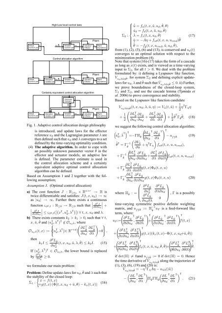
Fig. 1. Adaptive control allocation design philosophy is introduced, and update laws for the effector reference u d and the Lagrangian parameter are then dened such that u d and converges to a set dened by the time-varying optimality condition. (4) The adaptive algorithm. In order to cope with an possibly unknown parameter vector in the effector and actuator models, an adaptive law is dened. The parameter estimate is used in the control allocation scheme and a certainty equivalent adaptive optimal control allocation algorithm can be dened. Based on Assumption 1 and 2 together with the following assumption; Assumption 3. (Optimal control allocation) a) The cost function J : R t0 R nr ! R is twice differentiable and satises: J(t; x; u d ) ! 1 as ju d j ! 1. Further there exists a continuous function & @2 J : R 0 ! R 0 such that @2 J @t@u d + @2 J @x@u d &@ 2 J( x T ; u T d ; T ) 8 t; x; u d and : b) There exists constants k 2 > k 1 > 0, such that 8 t; x; ~u; ^ and (u T d ; T ) T =2 O ud ; where ( ! ) O ud (t; x) := u T d; T 2 R r+d @L T^ ; @LT^ =0 ; @u d @ then k 1 I @2 L^ @u 2 (t; x; u d ; ~u; ; ^) k 2 I: (15) d If (u T d ; T ) T 2 O ud ; the lower bound is replaced by @2 L^ @u 2 d 0. we formulate our main problem: Problem: Dene update-laws for u d , ^ and such that the stability of the closed loop: _x = f(t; x) 1 : (16) +g(t; x) ((t; x; u d + ~u; ) k x (t; x)) 8 _~u = f ~u (t; x; ~u; u d ; ^; ) >< _u d = f d (t; x; ~u; u d ; ^) 2 : _ = f (t; x; u d ; ^) _ = A + f u (t; x; u; u cmd ) >: ~ (17) _~ = f^(t; x; u cmd ; ~u; u d ; ^); from (1), (2), (3), (6) and (13), is conserved and u d (t) converges to an optimal solution with respect to the minimization problem (4). Note that system (16)-(17) takes the form of a cascade as long as x(t) exists, and is viewed as a time-varying input to 2 ; for all t > 0: We deal with the problem formulated by: i) dening a Lyapunov like function, V ud ~u ~ ; for system 2 and dening explicit updatelaws for u d , and ~ such that V _ ud ~u ~ 0: ii) Further, we prove boundedness of the closed-loop system, 1 and 2 ; and use the cascade lemma (Tjønnås et al. 2006) to prove convergence and stability. Based on the Lyapunov like function candidate V ud ~u ~ (t; x; u d; ; ~u; ) := V ~u (t; ~u) + 1 2 T ! + 1 @L T^ @L^ + @LT^ @L^ + 1 2 @u d @u d @ @ 2 ~ T ~ ~ ; (18) we suggest the following control allocation algorithm: ! _u T d; _ T T T = @L^ H^ ; @L^ T T u @u d @ ff^ (19) _^ T = 1 @V~u ~ @~u + T f u (t; x; u; u cmd ); ! @L T^ + 1 @ 2 L^ + @LT^ @ 2 L^ f ~ u (t; x; u; u cmd ) @u d @~u@u d @ @~u@ @L T^ + 1 @ 2 L^ ~ @ @L T^ + 1 @ 2 L^ ~ @x@ g(t; x) (t; x; u) g(t; x) (t; x; u) (20) @u d @x@u d 0 1 @ 2 L^ @u 2 d @ 2 L^ @ 2 L^ where H^ : = B @@u d C @ A ; is a possibly 0 @u d @ time-varying symmetric positive denite weighting matrix, and u ff^ := H 1 ^ u F is a feed-forward like term, where: ! ; @2 T T ! L^ + @2 T L^ ; @2 T T L^ f(t; x) @t@ @x@u d @x@ u F := @2 T L^ @t@u d + @2 L T^ ; @2 L T^ @x@u d @x@ + @2 L T^ @~u@u d ; @2 L T^ @~u@ ! T g(t; x)(k x (t; x) (t; x; u d +~u; ^)) ! T f ~u (t; x; ~u; u d ; ^; ^)+ @2 L T^ ! ; @2 L T_^: T^ @^@u d @^@ if det(H) 6= 0;and u ff^ := 0 if det(H) = 0: Hence the time derivative of V ud ~u ~ along the trajectories of (1), (3), (6), (19) and (20) is: _V ud ~u ~ = T A ~u3 (j~uj) @L T ; @L T @L T H^ H^ ; @L T T : (21) @u d @ @u d @
Page 1: ON OPTIMIZING NONLINEAR ADAPTIVE CO
Page 5 and 6: T i ( x ; ! i ; i ) := T ni (! i )

ON OPTIMIZING NONLINEAR ADAPTIVE CONTROL ... - NTNU

You also want an ePaper? Increase the reach of your titles

Delete template?

Save as template?