Solid State Theory Exercise 2 Point groups and their representations ...

Solid State Theory
Exercise 2
FS 13
Prof. M. Sigrist
Point groups and their representations:
Energy bands of nearly free electrons on the fcc lattice
Let us consider almost free electrons on a face-centered cubic (fcc) lattice. The goal of
this exercise is to compute the lowest energy bands along the ∆-line using degenerate
perturbation theory and the machinery of group theory.
• What does the first Brillouin zone of the fcc look like? Include a sketch and label
the Γ and X points. The line connecting them is the above mentioned ∆-line.
The Bloch equation is written in Fourier space as
[ ]
2
2m (⃗ k + G) ⃗ 2 − ε n, ⃗ k
c ⃗G + ∑ G ⃗ ′
V ⃗G− ⃗ G ′c ⃗G ′ = 0. (1)
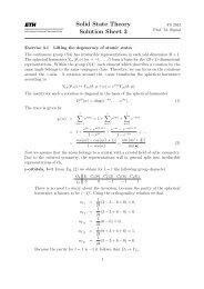
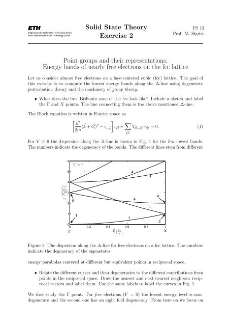
For V ≡ 0 the dispersion along the ∆-line is shown in Fig. 1 for the few lowest bands.
The numbers indicate the degeneracy of the bands. The different lines stem from different
6
V = 0
5
1
4
4
4
ε [ ¯h2 G 2
2m ]
3
2
8
1
1
1
2
0
0 0.2 0.4 0.6 0.8 1
⃗ k [
2π
Γ
a ]
X
4
1
4
Figure 1: The dispersion along the ∆-line for free electrons on a fcc lattice. The numbers
indicate the degeneracy of the eigenstates.
energy parabolas centered at different but equivalent points in reciprocal space.
• Relate the different curves and their degeneracies to the different contributions from
points in the reciprocal space. Draw the nearest and next nearest neighbour reciprocal
vectors and label them. Use the same labels to label the curves in Fig. 1.
We first study the Γ point. For free electrons (V = 0) the lowest energy level is nondegenerate
and the second one has an eight fold degeneracy. From here on we focus on

the second energy level.
As you found in the previous part, the 8-fold degeneracy stems from parabolas centered
at the 8 points connected to Γ by the following reciprocal lattice vectors:
⃗G 1 = G(1, 1, 1), G2 ⃗ = G(−1, 1, 1),
⃗G 3 = G(−1, −1, 1), G4 ⃗ = G(1, −1, 1),
⃗G 5 = G(1, 1, −1), G6 ⃗ = G(−1, 1, −1),
⃗G 7 = G(−1, −1, −1), G8 ⃗ = G(1, −1, −1),
(2)
where G = 2π . These vectors form an 8 dimensional Hilbertspace, and the eigenfunctions
a
are given by
ψ j (⃗r) = 〈⃗r| G ⃗ j 〉 = ei G ⃗ j·⃗r
√ . (3)
V
The point group of the cubic Bravais lattices (simple cubic, fcc, bcc) is denoted by O h
(symmetry group of a cube). Its character table is given in Tab. 1.
O h E C 3 (8) C4(3) 2 C 2 (6) C 4 (6) J JC 3 (8) JC4(3) 2 JC 2 (6) JC 4 (6)
[xyz] [zxy] [¯xȳz] [yx¯z] [ȳxz] [¯xȳ¯z] [¯z¯xȳ] [xy¯z] [ȳ¯xz] [y¯x¯z]
1 1 1 1 1 1 1 1 1 1
1 1 1 1 1 −1 −1 −1 −1 −1
1 1 1 −1 −1 1 1 1 −1 −1
1 1 1 −1 −1 −1 −1 −1 1 1
2 −1 2 0 0 2 −1 2 0 0
2 −1 2 0 0 2 1 −2 0 0
3 0 −1 −1 1 3 0 −1 −1 1
3 0 −1 −1 1 −3 0 1 1 −1
3 0 −1 1 −1 3 0 −1 1 −1
3 0 −1 1 −1 −3 0 1 −1 1
χ Γ
+
1
χ Γ
−
1
χ Γ
+
2
χ Γ
−
2
χ Γ
+
12
χ Γ
−
12
χ Γ
+
15
χ Γ
−
15
χ Γ
+
25
χ Γ
−
25
Table 1: The character table of the cubic point group O h .
We will denote the eight-dimensional representation of O h defined on this subspace by Γ.
Find the irreducible representations contained in Γ. To this end, we compute the group
character χ Γ and use the character table of O h to show that
The representation Γ of O h on this subspace is defined as
where g ∈ O h .
Γ = Γ + 1 ⊕ Γ − 2 ⊕ Γ − 15 ⊕ Γ + 25. (4)
ˆΓ(g)| ⃗ G j 〉 = |g ⃗ G j 〉 (5)
• How does a real space vector ⃗r change under the action of such a symmetry operation?

It is easy to see that each element of the cubic point group simply permutes the G ⃗ j ’s. For
example, a rotation by π/2 around the z-axis is represented as
⎛
⎞
0 1 0 0 0 0 0 0
0 0 1 0 0 0 0 0
0 0 0 1 0 0 0 0
Rπ/2 z =
1 0 0 0 0 0 0 0
0 0 0 0 0 1 0 0
.
⎜ 0 0 0 0 0 0 1 0
⎟
⎝ 0 0 0 0 0 0 0 1 ⎠
0 0 0 0 1 0 0 0
The character of this transformation is χ Γ (Rπ/2 z ) = tr(Rz π/2
) = 0. Clearly, in order to find
all the characters of the representation Γ defined by Eq. (5) we don’t have to compute all
the matrices. Instead, we simply have to know how many of the G ⃗ i ’s are invariant under
a certain element.
• Explain shortly why one obtains the character in this case simply by counting the
invariant ⃗ G i ’s.
It is sufficient to consider one element of each conjugacy class. In the following, J will
denote the inversion, C 3 (8) the conjugacy class of rotations by 2π/3 around one of the
diagonals of the cube, C 4 (6) the conjugacy class of the rotations by π/2, C 2 (6) the conjugacy
class of rotations by π around an axis through the edges of the cube and C 2 4(3)
the conjugacy class of the rotations by π around an axis through surface of the cube.
(The number in brackets denotes the number of elements in the corresponding conjugacy
class.)
• Complete the following character table
E C 3 (8) C 2 4(3) C 2 (6) C 4 (6) J JC 3 (8) JC 2 4(3) JC 2 (6) JC 4 (6)
χ Γ . . . . 0 . . . . .
Using the orthogonality of the characters we can compute how many times the irreducible
representation Γ ± i is contained in Γ:
〈 〉
n Γ
± = χ Γ , χ
i
Γ
± := 1 ∑
χ Γ (g)χ
i |O h |
Γ
± (g) = 1 ∑
χ Γ (C n )χ
i |O h |
Γ
± (C n) |C n |
i
g∈O h C n
where C n denotes the conjugacy classes of O h , |C n | the order of the conjugacy class (e.g.
C 3 (8) has 8 elements) and |O h | = 48 the order of the group. One computes
n Γ
+ = 1 (8 + 2 × 8 + 4 × 6) = 1 (6)
1 48
Similarly, one finds n Γ
− = n
2 Γ − = n 15 Γ + = 1, while all the others are 0. Therefore,
25
Γ = Γ + 1 ⊕ Γ − 2 ⊕ Γ − 15 ⊕ Γ + 25. (7)
A finite periodic potential will in general split the second energy level at the Γ point.
Applying degenerate perturbation theory to the Bloch equation [Eq. (1.27) in the lecture
notes] leads to an 8 × 8 matrix with off-diagonal elements u = V 4π
(1,1,1), v = V 4π (1,0,0) and
a a
w = V 4π
(1,1,0).
a

• Check for yourself that this matrix is given by
⎛
⎞
E 0 − ε v w v v w u w
v E 0 − ε v w w v w u
w v E 0 − ε v u w v w
A =
v w v E 0 − ε w u w v
v w u w E 0 − ε v w v
⎜ w v w u v E 0 − ε v w
⎟
⎝ u w v w w v E 0 − ε v ⎠
w u w v v w v E 0 − ε
This matrix can be diagonalized by going into the symmetry subspaces. We will show
that for the energies and the wave functions one finds
where E 0 = 2
2m 3( 2π a )2 .
Γ + 1 : E 0 + u + 3v + 3w cos ( 2π
x) cos ( 2π
y) cos ( 2π
z) ;
a a a
Γ − 2 : E 0 − u − 3v + 3w sin ( 2π
x) sin ( 2π
y) sin ( 2π
z) ;
a a a
Γ − 15 : E 0 − u + v − w { sin ( 2π
x) cos ( 2π
y) cos ( 2π
z) , cyclic } { (
;
a a a
Γ + 25 : E 0 + u − v − w cos 2π x) sin ( 2π
y) sin ( 2π
z) , cyclic } ;
a a a
(8)
For V ≠ 0 the wave functions ψ j (⃗r) mix. Applying degenerate perturbation theory means
we have to solve the secular equation:
det A = 0
which has to be solved for ε. By projecting suitable vectors onto the symmetry subspaces
found in a) one can systematically construct an eigenbasis and with it find the energies.
However, for relatively small systems it is often possible to guess the correct eigenfunctions
using some symmetry properties of the basis functions of the irreducible representations.
Since the physical eigenfunctions have to be periodic in real space it is natural to use
combinations of cos(Gx) and sin(Gx) etc.
1. The eigenfunction belonging to the subset Γ + 1 has to be totally symmetric under
all the operations. Therefore, e 1 = ( 1 1 1 1 1 1 1 1 ) is an eigenvector
with energy ε 1 = E 0 + u + 3v + 3w. The physical eigenfunction can be found as
f 1 (⃗r) ∼ ∑ j ei ⃗ G j ⃗r ∼ cos(Gx) cos(Gy) cos(Gz).
2. For Γ − 15 we need three functions which are odd under the inversion operation ⃗r → −⃗r.
We therefore need an odd number of sin’s. What is left are the combinations
f 3 (⃗r) ∼ sin(Gx) cos(Gy) cos(Gz), f 4 (⃗r) ∼ cos(Gx) sin(Gy) cos(Gz) and f 5 (⃗r) ∼
cos(Gx) cos(Gy) sin(Gz). They correspond to the following vectors
e 3 = ( 1 −1 −1 1 1 −1 −1 1 )
e 4 = ( 1 1 −1 −1 1 1 −1 −1 )
e 5 = ( 1 1 1 1 −1 −1 −1 −1 )
with energy ε 3−5 = E 0 − u + v − w.
• Using the character table, repeat the above steps to find the eigenfunction f 2 (⃗r)
belonging to the subset Γ − 2 . Also compute its energy.

• Again, repeat the above for the eigenfunctions and energy belonging to the subspace
Γ + 25.
How do the irreducible representations split on the ∆-line? The ∆-line is defined by the
points ⃗ k = 2π (0, 0, δ), 0 ≤ δ ≤ 1 (i.e. we choose the z-axis going through X). Use the
a
character table of C 4v .
C 4v E C 2 (1) C 4 (2) σ v (2) σ d (2)
[xyz] [¯xȳz] [y¯xz] [¯xyz] [yxz]
χ ∆1 1 1 1 1 1
χ ∆2 1 1 1 −1 −1
χ ∆3 1 1 −1 1 −1
χ ∆4 1 1 −1 −1 1
χ ∆5 2 −2 0 0 0
Table 2: The character table of C 4v .
On the ∆-line the number of symmetry operations which leave the ⃗ k-vector invariant is
reduced. Only the rotations around the z-axis or the reflections on mirror planes containing
the z-axis leaves the ⃗ k-vector invariant. The ”small group” is now C 4v , the symmetry
group of a square. Under these reduced operations, the irreducible representations of O h
will in general split into irreducible representations of C 4v .
(i) Of course, the trivial representation of O h changes to the trivial representation of C 4v :
Γ + 1 ↦→ ∆ 1 .
(ii) Under the operations of C 4v the group character of Γ − 2 is easily found using the
properties of the basis function f 2 (⃗r):
C 4v E C4 2 C 4 σ v σ d
1 1 −1 −1 1
χ Γ
−
2
This is the character of ∆ 4 and therefore Γ − 2 ↦→ ∆ 4 .
(9)
• Using the basis functions {f 3 (⃗r), f 4 (⃗r), f 5 (⃗r)}, find the matrix belonging to the different
conjugacy classes. For example, a matrix belonging to the conjugacy class
C 4 ([y¯xz]) would be computed as follows. Consider the function f 3 (x, y, z); then
performing a C 4 rotation, this function becomes f 3 (y, −x, z). Inspection of this latter
function shows that it is identical to f 4 (x, y, z), explaining the first row of the
following matrix:
⎛ ⎞
0 1 0
C 4 ([y¯xz]) = ⎝ −1 0 0 ⎠ (10)
0 0 1
It is imporant to realize that this transformation acts on the basis functions (imagine
a vector (f 3 , f 4 , f 5 ) on which this matrix acts). In this case, the matrix can also
be found by considering simply the vector (x, y, z) → (y, −x, z)).
Then compute the group character and extract the irreducible representations by
using the orthogonality of the characters (as in the first part of this exercise).

C 4v E C4 2 C 4 σ v σ d
. . . . .
χ Γ
−
4
(11)
(iii) For Γ + 25 we will find in an analogous way
C 4v E C4 2 C 4 σ v σ d
3 −1 −1 −1 1
χ Γ
+
25
(12)
and therefore Γ + 5 ↦→ ∆ 4 ⊕ ∆ 5 .
Let us now consider the point X = 2π (0, 0, 1). The lowest level is two fold and the second
a
four fold degenerate for V = 0. Compute the energies and the wave functions for these
two levels.
( )
At the point X = 2π a 0 0 1 the symmetry is larger than along the ∆-line, but smaller
than the full group O h . It contains all the elements of O h which map z to z or to −z.
This group is called D 4h . In order to compute the lifting of the degeneracy of the lowest
two levels we can simply diagonalize the corresponding matrices. The irreducible representation
of D 4h are given in Table 3.
even basis function d X odd basis function d X
X + 1 1 1 X − 1 xyz(x 2 − y 2 ) 1
X + 2 xy(x 2 − y 2 ) 1 X − 2 z 1
X + 3 x 2 − y 2 1 X − 3 xyz 1
X + 4 xy 1 X − 4 z(x 2 − y 2 ) 1
X + 5 zx, zy 2 X − 5 x, y 1
Table 3: Irreducible representations of D 4h , split according to their parity (z → z or
z → −z. The dimension of the irreducible representation is indicated in the column
labeled d X .
Lowest level: The G-vectors ⃗ entering the Bloch equation in lowest order in the periodic
potential are G ⃗ 0 = 0 and G ⃗ 9 = 2G(0, 0, 1). Furthermore, v = V ⃗G0 −G ⃗ 9
enters as well.
• Construct the secular equation, and find the eigenvectors.
The eigenfunctions you find from the vectors are cos Gz and sin Gz, respectively. Comparing
this to the irreducible representations of D 4h we find that e 1 corresponds to X + 1
and e 2 to X − 2 .
Second-lowest level: The G-vectors ⃗ entering the Bloch equation in lowest order in the
periodic potential are G ⃗ 1 to G ⃗ 4 and we have to diagonalize the matrix
⎛
⎞
2 2 G 2
v w v
2m v 2 2 G 2
v w
⎜
2m ⎝ w v 2 2 G ⎟
2
v ⎠ .
2m
v w v 2 2 G 2
2m

Here, v and w have the same meaning as above. From the symmetry of the matrix it is
clear that the eigenvectors are of the form (a, b, b, a) and (a, b, −b, −a). One then finds
e 1 = ( 1 1 1 1 ) and E 1 = 2 2 G 2
+ 2v + w,
2m
e 2 = ( 1 1 −1 −1 ) and E 2 = 2 2 G 2
2m − w,
e 3 = ( 1 −1 −1 1 ) and E 3 = 2 2 G 2
2m − w,
e 4 = ( 1 −1 1 −1 ) and E 4 = 2 2 G 2
− 2v + w.
2m
• Compare these results again to the eigenfunctions given in Table 3, and identify the
irreducible representations they belong to.
• Finally, sketch the energy bands between the Γ and the X point and compare it to
the free electron (V = 0 case). For an actual numerical calculation use the values
u = −0.05, v = 0.05 and w = 0.1 (in units of (2π)2
2ma 2 ).
Contact Person:
Evert van Nieuwenburg (HIT K 23.7)
evertv@itp.phys.ethz.ch