You Are the Traffic Jam: An Examination of Congestion Measures ...
You Are the Traffic Jam: An Examination of Congestion Measures ...
You Are the Traffic Jam: An Examination of Congestion Measures ...

Create successful ePaper yourself
Turn your PDF publications into a flip-book with our unique Google optimized e-Paper software.
<strong>You</strong> <strong>Are</strong> <strong>the</strong> <strong>Traffic</strong> <strong>Jam</strong>: <strong>An</strong> <strong>Examination</strong> <strong>of</strong> <strong>Congestion</strong> <strong>Measures</strong><br />
Robert L. Bertini<br />
Department <strong>of</strong> Civil & Environmental Engineering<br />
Portland State University<br />
P.O. Box 751<br />
Portland, OR 97207-0751<br />
Phone: 503-725-4249<br />
Fax: 503-725-5950<br />
Email: bertini@pdx.edu<br />
Submitted for presentation at <strong>the</strong><br />
85th <strong>An</strong>nual Meeting <strong>of</strong> <strong>the</strong> Transportation Research Board<br />
January 2006, Washington, D.C.<br />
7339 words<br />
November, 2005
Bertini 2<br />
ABSTRACT<br />
The objective <strong>of</strong> this paper is to discuss current definitions <strong>of</strong> metropolitan traffic congestion and<br />
ways it is currently measured. In addition, <strong>the</strong> accuracy and reliability <strong>of</strong> <strong>the</strong>se measures will be<br />
described along with a review <strong>of</strong> how congestion has been changing over <strong>the</strong> past several<br />
decades. First, <strong>the</strong> results <strong>of</strong> a survey among transportation pr<strong>of</strong>essionals are summarized to<br />
assist in framing <strong>the</strong> issue. Most respondents linked <strong>the</strong> measurement <strong>of</strong> congestion to <strong>the</strong><br />
increased travel time that occurs during peak periods. Roughly half <strong>of</strong> those surveyed felt that<br />
congestion measures are at least somewhat accurate, and about 80% <strong>of</strong> those surveyed feel that<br />
congestion has worsened over <strong>the</strong> past 20 years. The paper includes a literature review <strong>of</strong><br />
current trends in congestion definition and measurement, a discussion and short critique <strong>of</strong> one<br />
major congestion monitoring program, and presents some basic <strong>the</strong>ory about how traffic<br />
parameters are <strong>of</strong>ten measured over time and space. A brief description <strong>of</strong> possible congestion<br />
measures over corridors and entire door-to-door trips is provided. Additional analysis <strong>of</strong> recent<br />
congestion measures for entire metropolitan area is provided, using Portland, Oregon and<br />
Minneapolis, Minnesota as case examples. Some discussion <strong>of</strong> <strong>the</strong> stability <strong>of</strong> daily travel<br />
budgets and alternative viewpoints about congestion are provided along with some conclusions<br />
and perspectives for future research.
Bertini 3<br />
INTRODUCTION<br />
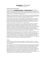
"<strong>You</strong>'re not stuck in a traffic jam, you are <strong>the</strong> jam." (1)<br />
<strong>Congestion</strong>—both in perception and in reality—impacts <strong>the</strong> movement <strong>of</strong> people and freight and<br />
is deeply tied to our history <strong>of</strong> high levels <strong>of</strong> accessibility and mobility. <strong>Traffic</strong> congestion<br />
wastes time and energy, causes pollution and stress, decreases productivity and imposes costs on<br />
society equal to 2-3% <strong>of</strong> our gross domestic product (GDP) (2). For 2002, it was estimated that<br />
congestion “wasted” $63.2 billion in 75 metropolitan areas because <strong>of</strong> extra time lost and fuel<br />
consumed, or $829 per person. (3) Some refer to <strong>the</strong>se estimates as misleading since <strong>the</strong> prospect<br />
<strong>of</strong> eliminating all congestion is “only a myth; congestion could never be eliminated completely.”<br />
(4). While some research emphasizes that “rush hour is longer than an hour in <strong>the</strong> morning and<br />
an hour in <strong>the</strong> evening and few people are ‘rushing’ anywhere,” o<strong>the</strong>rs say that “gridlock is not<br />
going to happen because people change what <strong>the</strong>y do long before it happens.” (5) Some view<br />
congestion as a “problem” that individual drivers are subject to, while o<strong>the</strong>rs emphasize that <strong>the</strong><br />
users <strong>of</strong> transportation networks “not only experience congestion, <strong>the</strong>y create it.” It has been<br />
shown that most people make travel decisions based on an expectation <strong>of</strong> experiencing a certain<br />
amount <strong>of</strong> congestion; however most people do not consider <strong>the</strong> cost that <strong>the</strong>ir travel imposes on<br />
o<strong>the</strong>rs by adding to <strong>the</strong> congested conditions. The objective <strong>of</strong> this paper is to discuss current<br />
definitions <strong>of</strong> metropolitan traffic congestion and ways it is currently measured, and to<br />
summarize a larger study contained in (6). In addition, <strong>the</strong> accuracy and reliability <strong>of</strong> <strong>the</strong>se<br />
measures will be described along with a review <strong>of</strong> how congestion has been changing over <strong>the</strong><br />
past few decades.<br />
FRAMING THE ISSUE<br />
<strong>Congestion</strong> measurement focuses on system performance and measures <strong>of</strong> people’s experiences.<br />
To assist in framing <strong>the</strong> issues, an unscientific web-based survey about metropolitan area<br />
congestion was distributed by email to more than 3,500 transportation pr<strong>of</strong>essionals and<br />
academics, and a total <strong>of</strong> 480 responses were received. The survey, conducted specifically for<br />
this paper, asked four qualitative questions:<br />
1. How do you define congestion in metropolitan areas?<br />
2. How is congestion in metropolitan areas measured?<br />
3. How accurate or reliable are traffic congestion measurements?<br />
4. How has metropolitan traffic congestion been changing over <strong>the</strong> past two decades?<br />
Respondents were provided with an opportunity to comment on congestion in general. The<br />
survey results are described below and are used to motivate later elements <strong>of</strong> <strong>the</strong> paper.<br />
Definition <strong>of</strong> <strong>Congestion</strong><br />
For <strong>the</strong> first question 557 responses were received (separate definitions for freeways and<br />
signalized intersections). As shown in Figure 1, survey respondents mentioned time, speed,<br />
volume, level <strong>of</strong> service (LOS) and traffic signal cycle failure (meaning that one has to wait<br />
through more than one cycle to clear <strong>the</strong> queue) as primary definitions <strong>of</strong> congestion. Typical<br />
LOS measures include volume/capacity, density, delay, number <strong>of</strong> stops, among o<strong>the</strong>rs. Most<br />
responses included a “time” component—travel time, speed, cycle failure and LOS are all related<br />
to <strong>the</strong> fact that users experience additional travel time due to congestion. Some definitions <strong>of</strong><br />
congestion rely on point measures (e.g., volume and time mean speed) and some rely on spatial<br />
measures (travel time, density and space mean speed).
Bertini 4<br />
How Is <strong>Congestion</strong> Defined?<br />
(n=557)<br />
Cycle<br />
O<strong>the</strong>r<br />
Time<br />
Failure<br />
4%<br />
18%<br />
16%<br />
How Is <strong>Congestion</strong> Measured?<br />
(n=682)<br />
O<strong>the</strong>r<br />
Density<br />
5%<br />
1%<br />
Travel<br />
Queue<br />
Time<br />
Length<br />
14%<br />
4%<br />
LOS<br />
15%<br />
Delay<br />
29%<br />
Speed<br />
13%<br />
Vol<br />
19%<br />
Speed<br />
28%<br />
LOS<br />
20%<br />
V/C<br />
14%<br />
How Accurate <strong>Are</strong> <strong>Congestion</strong><br />
<strong>Measures</strong>? (n=525)<br />
Variable<br />
20%<br />
Relative<br />
4%<br />
Subjective<br />
5%<br />
Unknown<br />
6%<br />
Inaccurate<br />
14%<br />
Accurate<br />
18%<br />
Somewhat<br />
Accurate<br />
33%<br />
FIGURE 1 <strong>Congestion</strong> survey results.<br />
More<br />
Available<br />
Options<br />
6%<br />
How Has <strong>Congestion</strong><br />
Changed? (n=446)<br />
Varies<br />
Not<br />
5%<br />
Known<br />
3%<br />
Better<br />
3%<br />
Flat<br />
4%<br />
Worse<br />
79%<br />
Point-related definitions include vehicle count (flow) and time mean speed extracted<br />
from point detectors (extrapolated over a segment to estimate link travel time). Spatial<br />
definitions include density, queue length and actual segment travel time (recorded by a probe<br />
vehicle). Survey comments noted that “if we want to reduce congestion we need to be able to<br />
define it and quantify it.” Some were willing to define congestion as “anything below <strong>the</strong> posted<br />
speed limit,” or below some “speed threshold (e.g.,
Bertini 5<br />
definition <strong>of</strong> road congestion, but that an appropriate definition might be: “<strong>the</strong> impedance<br />
vehicles impose on each o<strong>the</strong>r, due to <strong>the</strong> speed-flow relationship, in conditions where <strong>the</strong> use <strong>of</strong><br />
a transport system approaches its capacity.” (8) Finally, a survey conducted by <strong>the</strong> National<br />
Associations Working Group for ITS included a response describing <strong>the</strong> difficulty in defining<br />
congestion: “you know it when you see it—and <strong>the</strong> severity <strong>of</strong> <strong>the</strong> problem should be judged by<br />
<strong>the</strong> commonly accepted community standards.” (9)<br />
Measurement <strong>of</strong> <strong>Congestion</strong><br />
There were 682 responses to <strong>the</strong> second question (multiple responses). Per Figure 1, most<br />
responses were related to time: delay, speed, travel time and LOS, all <strong>of</strong> which include <strong>the</strong> notion<br />
that actual travel time can be a primary measure <strong>of</strong> congestion. O<strong>the</strong>r measures included<br />
volume/capacity (point measure) and queue length and density (spatial measures). Responses in<br />
<strong>the</strong> “O<strong>the</strong>r” category included number <strong>of</strong> stops and travel time reliability. One responded<br />
summed up <strong>the</strong> issue by stating “it is never truly measured.” The literature includes a wide array<br />
<strong>of</strong> possible congestion measures including: volume/capacity (disregards duration), VKT,<br />
VKT/lane km, speed, occupancy, travel time, delay, LOS and reliability. In <strong>the</strong> U.K. survey<br />
several helpful measures <strong>of</strong> congestion were identified: delay (51%); risk <strong>of</strong> delay (20%);<br />
average speed (18%); and amount <strong>of</strong> time stationary or less than 10 mph (11%).<br />
Accuracy and Reliability <strong>of</strong> <strong>Congestion</strong> Measurements<br />
There were 525 responses to question three, indicating mixed feelings about <strong>the</strong><br />
accuracy/reliability <strong>of</strong> congestion measurements. About half <strong>of</strong> <strong>the</strong> responses indicated that <strong>the</strong><br />
measurements are accurate or somewhat accurate, while <strong>the</strong> o<strong>the</strong>r half indicated that <strong>the</strong>y are<br />
inaccurate or variable. Many comments indicated that measurements are <strong>of</strong>ten based on very<br />
small sample sizes, that <strong>the</strong>y are relative and variable and that <strong>the</strong>y should be presented with<br />
confidence intervals ra<strong>the</strong>r than purely deterministic values. One comment stated that congestion<br />
measurements are “reasonably accurate despite <strong>the</strong> fact that <strong>the</strong>y measure <strong>the</strong> wrong things,”<br />
while ano<strong>the</strong>r stated that “congestion perception is a personal thing based on personal<br />
experiences and anecdotes.” Finally, one comment indicated that “<strong>the</strong> result is really just a<br />
snapshot in time.”<br />
Changes in <strong>Congestion</strong><br />
For <strong>the</strong> final survey question most respondents indicated that congestion has worsened. Some<br />
respondents indicated that more transportation options (such as transit and intelligent<br />
transportation systems) are now available and some indicated that congestion has gotten better.<br />
Respondents noted that <strong>the</strong> impact <strong>of</strong> congestion has increased in both spatial and temporal<br />
dimensions, including <strong>the</strong> spread <strong>of</strong> peak periods. O<strong>the</strong>rs pointed out that change has been<br />
relative, depending on <strong>the</strong> area and on <strong>the</strong> user. Some respondents indicated that drivers have<br />
been conditioned to tolerate more congestion.<br />
Several responses pointed out that <strong>the</strong> congestion will always be a by-product <strong>of</strong> a<br />
healthy, vibrant urban area. It was pointed out that traditional traffic/transportation engineering<br />
antidotes to congestion have been reactive, and that roadways are not improved until <strong>the</strong>re is a<br />
problem. <strong>An</strong>o<strong>the</strong>r comment stated that “current conceptions <strong>of</strong> congestion have more to do with<br />
preserving <strong>the</strong> world as it was, ra<strong>the</strong>r than preparing us for <strong>the</strong> world as it will be,” and ano<strong>the</strong>r<br />
stated that <strong>the</strong>re is “too much focus on congestion, <strong>the</strong>re should be more attention to<br />
accessibility. What can people get to in a reasonable period <strong>of</strong> time (20-30 minutes)?” Several
Bertini 6<br />
respondents indicated that <strong>the</strong>re has been a transformation from <strong>the</strong> mentality that you can “build<br />
your way out <strong>of</strong> congestion” to <strong>the</strong> point where o<strong>the</strong>r options such as HOV lanes and reversible<br />
lanes” are available.<br />
LITERATURE REVIEW<br />
The survey results motivated a comprehensive literature review in order to explore current<br />
federal, state and local efforts to define and quantify congestion. A full version can be found in<br />
(6).<br />
Federal Definition and Monitoring<br />
The Federal Highway Administration (FHWA) defines traffic congestion as: “<strong>the</strong> level at which<br />
transportation system performance is no longer acceptable due to traffic interference.” Because<br />
<strong>the</strong>re is a relative sense to <strong>the</strong> word “congestion,” <strong>the</strong> FHWA continues <strong>the</strong>ir definition by stating<br />
that “<strong>the</strong> level <strong>of</strong> system performance may vary by type <strong>of</strong> transportation facility, geographic<br />
location (metropolitan area or sub-area, rural area), and/or time <strong>of</strong> day,” in addition to o<strong>the</strong>r<br />
variations by event or season. (10) The definition <strong>of</strong> congestion is imprecise and is made more<br />
difficult since people have different perceptions and expectations <strong>of</strong> how <strong>the</strong> system should<br />
perform based on whe<strong>the</strong>r <strong>the</strong>y are in rural or urban areas, in peak/<strong>of</strong>f peak, and as a result <strong>of</strong> <strong>the</strong><br />
history <strong>of</strong> an area.<br />
<strong>Congestion</strong> can vary since demand (day <strong>of</strong> week, time <strong>of</strong> day, season, recreational,<br />
special events, evacuations, special events) and capacity (incidents, work zones, wea<strong>the</strong>r) are<br />
changing. Most researchers agree that recurrent congestion (due to demand exceeding capacity<br />
(40%) and poor signal timing (5%)) makes up about half <strong>of</strong> <strong>the</strong> total delay experienced by<br />
motorists, while nonrecurrent congestion (due to work zones (10%), incidents (30%) and wea<strong>the</strong>r<br />
(15%)) makes up <strong>the</strong> o<strong>the</strong>r half.<br />
Based on U.S. Census data, an extensive analysis <strong>of</strong> commuting patterns has been<br />
conducted (11). In this analysis <strong>of</strong> journey to work data, <strong>the</strong>re seem to be several thresholds for<br />
unacceptable congestion occurring: if less than half <strong>of</strong> <strong>the</strong> population can commute to work in<br />
less than 20 minutes or if more than 10% <strong>of</strong> <strong>the</strong> population can commute to work in more than<br />
60 minutes. It is apparent that several agencies use <strong>the</strong> term “acceptable congestion,” but clearly<br />
this can mean different things to different people and at different times and locations. In this<br />
context, it has been argued that individuals and firms may choose to locate in a congested area<br />
due to easier access to o<strong>the</strong>r individuals and firms. (12) This highlights <strong>the</strong> need to consider <strong>the</strong><br />
interaction between transportation and land use when attempting to define congestion.<br />
A recent syn<strong>the</strong>sis examined more than 70 possible performance measures for monitoring<br />
highway segments and systems (13). From users’ perspectives, key measures for reporting <strong>the</strong><br />
quantity <strong>of</strong> travel included: person-kilometers traveled, truck-kilometers traveled, VKT, persons<br />
moved, trucks moved and vehicles moved. In terms <strong>of</strong> <strong>the</strong> quality <strong>of</strong> travel, key measures<br />
included: average speed weighted by person-kilometers traveled, average door-to-door travel<br />
time, travel time predictability, travel time reliability (percent <strong>of</strong> trips that arrive in acceptable<br />
time), average delay (total, recurring and incident-based) and LOS.<br />
O<strong>the</strong>r <strong>Congestion</strong> Definitions and Monitoring<br />
Transportation agencies have adopted definitions <strong>of</strong> congestion for <strong>the</strong>ir purposes. INCOG, <strong>the</strong><br />
regional council <strong>of</strong> governments in Tulsa, Oklahoma defines congestion as “travel time or delay<br />
in excess <strong>of</strong> that normally incurred under light or free-flow travel conditions.” (14) In Rhode
Bertini 7<br />
Island, <strong>the</strong> state DOT recognizes that “congestion can mean a lot <strong>of</strong> different things to different<br />
people.” As a result, <strong>the</strong> state attempts to use objective congestion performance measures such as<br />
percent travel under posted speed and volume/capacity ratios. In Cape Cod, Massachusetts, a<br />
traffic congestion indicator is used to track average annual daily bridge crossings over <strong>the</strong><br />
Sagamore and Bourne bridges. (15) This very simple measure was chosen for this island<br />
community since it is appropriate, easy to measure, and since historic data are available to<br />
monitor long-term trends. In <strong>the</strong> State <strong>of</strong> Oregon, <strong>the</strong> 1991 Transportation Planning Rule (TPR)<br />
uses VKT as a primary metric, with a goal <strong>of</strong> reducing VKT by 20% per capita in metropolitan<br />
areas by 2025.<br />
In Minnesota, freeway congestion is defined as traffic is flowing below 45 mph for any<br />
length <strong>of</strong> time in any direction, between 6:00 a.m. and 9:00 a.m. or 2:00 p.m. and 7:00 p.m. on<br />
weekdays. Michigan defines freeway congestion in terms <strong>of</strong> LOS F, when <strong>the</strong> volume/capacity<br />
ratio is greater than or equal to one. Since <strong>the</strong> function <strong>of</strong> <strong>the</strong> transportation system is to provide<br />
transport <strong>of</strong> people and goods, and its benefits are a function <strong>of</strong> <strong>the</strong> number <strong>of</strong> trips served, in<br />
California “congestion” is defined as <strong>the</strong> state when traffic flow and <strong>the</strong> number <strong>of</strong> trips are<br />
reduced. The California Department <strong>of</strong> Transportation (Caltrans) defines congestion as occurring<br />
on a freeway when <strong>the</strong> average speed drops below 35 mph for 15 minutes or more on a typical<br />
weekday. There is currently a proposal to change <strong>the</strong> definition <strong>of</strong> congestion to be measured as<br />
<strong>the</strong> time spent driving below 60 mph, based on analysis <strong>of</strong> 3363 loop detectors at 1324 locations<br />
as part <strong>of</strong> <strong>the</strong> California Performance Measurement System (PeMS) database (16). The State <strong>of</strong><br />
Washington DOT provides congestion information (in plain English) that uses real time<br />
measurements, reports on recurrent congestion (due to inadequate capacity) separately from<br />
nonrecurrent congestion (due to incidents). This includes <strong>the</strong> measurement <strong>of</strong> volumes, speeds,<br />
congestion frequency, and geographical extent <strong>of</strong> congestion, travel time and reliability. The<br />
Washington DOT also focuses on travel time reliability and predictability by presenting a “worst<br />
case” travel time for a set <strong>of</strong> corridors such that commuters can expect to be on time for work 19<br />
out <strong>of</strong> 20 working days a month (95 percent <strong>of</strong> trips), if <strong>the</strong>y allow for <strong>the</strong> calculated travel time.<br />
(17)<br />
The Urban <strong>Congestion</strong> Report<br />
The Urban Mobility Report (UMR) (3) is sponsored by a consortium <strong>of</strong> state departments <strong>of</strong><br />
transportation and several interest groups, has been conducted by <strong>the</strong> Texas Transportation<br />
Institute since 1982 (18) and tracks congestion patterns in <strong>the</strong> 75 largest U.S. metropolitan areas.<br />
The main mission <strong>of</strong> <strong>the</strong> UMR is to convert traffic counts to speeds, so that delay can be<br />
computed. Since 2002, <strong>the</strong> UMR has also reported on <strong>the</strong> contributions <strong>of</strong> operational strategies<br />
(such as incident management and ramp metering) and public transportation have on reducing<br />
delay (18).<br />
The UMR uses several measured variables reported as part <strong>of</strong> <strong>the</strong> Highway Performance<br />
Monitoring System (HPMS). In support <strong>of</strong> <strong>the</strong> HPMS, states are required to report 70 data<br />
elements on pavement condition, traffic counts, and physical design characteristics for a<br />
statistical sample <strong>of</strong> about 100,000 highway sections. For some segments, traffic count data are<br />
available from continuous (usually hourly) automatic traffic recorder systems, while on o<strong>the</strong>r<br />
segments <strong>the</strong>se data are measured over 48 hour periods on a triennial basis. The UMR uses <strong>the</strong><br />
following measured and reported variables for its analysis (for facilities defined in <strong>the</strong> HPMS as<br />
freeways and principal arterials): population, Urban <strong>Are</strong>a Size, Segment Length, Number <strong>of</strong><br />
Lanes, Average Daily <strong>Traffic</strong> (ADT) and directional Factor.
Bertini 8<br />
The UMR takes <strong>the</strong>se measured parameters and follows some well-documented procedures<br />
toward <strong>the</strong> production <strong>of</strong> <strong>the</strong> performance measures listed above. In order to complete <strong>the</strong><br />
process, a number <strong>of</strong> assumptions and constants are used: including: vehicle occupancy (1.25),<br />
250 working days per year, consumer price index (CPI), value <strong>of</strong> time ($13.45), commercial<br />
vehicle operating cost ($71.05), 5% commercial vehicles, fuel cost, peak periods 6:00-9:30 am<br />
and 3:30-7:00 pm., 50% <strong>of</strong> daily travel in peak period, uncongested “supply” (vehicles per lane<br />
per day) 14,000 for freeways and 5,500 for principal arterials, piecewise linear relation between<br />
road congestion index (ratio <strong>of</strong> daily traffic volume to supply <strong>of</strong> roadway) and percent <strong>of</strong> daily<br />
travel in congested conditions, relation between ADT and speed for freeway (peak and <strong>of</strong>f peak<br />
direction) and arterial (peak and <strong>of</strong>f peak direction), and free flow speed (96 km/h (60 mph) for<br />
freeways and 56 km/h (35 mph) for principal arterials).<br />
Given <strong>the</strong> measured or estimated traffic counts, data describing <strong>the</strong> length and numbers <strong>of</strong><br />
lanes for each freeway and principal arterial segment and <strong>the</strong> constants described above, <strong>the</strong><br />
UMR <strong>the</strong>n computes nine derived variables for each metropolitan area: daily VKT by facility<br />
type, lane miles by facility type, road congestion index (RCI), percent <strong>of</strong> congested travel during<br />
peak period, VKT by congestion level and direction, segment speed by congestion level and<br />
direction, delay, travel rate (minutes/km) by facility type (actual and free flow), and travel rate<br />
index (TRI).<br />
Given <strong>the</strong> count based estimates <strong>of</strong> speed, and assuming free flow speeds by facility type,<br />
<strong>the</strong> UMR reports four primary performance measures: annual delay per traveller, travel time<br />
index (ratio <strong>of</strong> travel time in <strong>the</strong> peak period to that in free flow conditions), travel delay, excess<br />
fuel consumed and congestion cost.<br />
UMR results are based on traffic count data that were originally collected for system<br />
monitoring. No actual traffic speeds or measures extracted from real transportation system users<br />
are included. The UMR leverages existing data sources (using 6 measured variables and 13<br />
constant values or relations). With this review <strong>of</strong> <strong>the</strong> literature in mind, <strong>the</strong>re are some basic<br />
<strong>the</strong>oretical issues that should be explored, so that various metrics and <strong>the</strong>ir derivations can be<br />
better understood.<br />
SOME BASIC THEORY<br />
Having reviewed <strong>the</strong> literature, it is clear that many common traffic measurements are derived<br />
from <strong>the</strong> basic traffic flow parameters—flow, density and speed. This section describes how<br />
<strong>the</strong>se fundamental measures can be applied at <strong>the</strong> level <strong>of</strong> <strong>the</strong> roadway segment, a corridor and<br />
over an entire door-to-door trip.<br />
Segment Level<br />
Figure 2 illustrates some basic points about traffic flow. In Figure 2(a), a set <strong>of</strong> vehicle<br />
trajectories on a time-space plane is shown in <strong>the</strong> context <strong>of</strong> a roadside observer (or detector) at<br />
location x. (19) During time interval t, an observer would count 7 vehicles passing point x. Flow,<br />
a point measure, is defined as <strong>the</strong> number <strong>of</strong> vehicles that pass a point during a particular time<br />
interval; in this case 7/t, usually expressed in vehicles/hour. Under certain circumstances <strong>the</strong><br />
“capacity” <strong>of</strong> <strong>the</strong> highway at point x might be estimated, and <strong>the</strong> actual measured volume could<br />
be compared to that <strong>the</strong>oretical capacity value in <strong>the</strong> form <strong>of</strong> a volume/capacity ratio. Speed<br />
could also be measured at point x, for example by a radar gun. If <strong>the</strong> arithmetic average <strong>of</strong> <strong>the</strong><br />
speeds measured at a point is taken over a measurement interval t, this is called <strong>the</strong> time mean<br />
speed.
Bertini 9<br />
Figure 2(b), which also shows a set <strong>of</strong> vehicle trajectories on a time-space plane,<br />
illustrates that some key traffic flow parameters are measured over distance. For example at time<br />
j, <strong>the</strong> number <strong>of</strong> vehicles on <strong>the</strong> segment d at that instant would be counted as six vehicles. The<br />
density at time j is <strong>the</strong> number <strong>of</strong> vehicles on <strong>the</strong> section at that time divided by <strong>the</strong> section<br />
length, in this case 6/d, usually expressed in vehicles/km. The actual travel times <strong>of</strong> vehicles can<br />
also be recorded over space; in this case for vehicle i, its travel time is shown as v i . The free<br />
flow travel time for segment d might be assumed to be v f . Therefore, for vehicle i on this<br />
roadway segment <strong>the</strong> delay is defined as v i -v f .<br />
v e = Extrapolated Travel Time<br />
v f = Free Flow Travel Time<br />
ve-vf = Delay<br />
i<br />
v i<br />
= Actual Travel Time<br />
v f<br />
= Free Flow Travel Time v-v i f = Delay<br />
i<br />
Distance<br />
Distance<br />
x<br />
Free<br />
Flow<br />
Speed<br />
Speed<br />
d = Segment Distance<br />
Time<br />
t = Measurement Interval<br />
Point <strong>Measures</strong><br />
(a)<br />
FIGURE 2 Segment level measures <strong>of</strong> congestion.<br />
j<br />
Spatial <strong>Measures</strong><br />
(b)<br />
Time<br />
Corridor Level<br />
It is possible to compute congestion-related measures over a larger freeway corridor where more<br />
detection locations are available. Travel time can be calculated from real-time or archived<br />
freeway sensor data by extrapolating a measured speed value over an influence area (segment).<br />
For example, Figure 3(a) shows travel time versus time for one day on northbound Interstate 5 in<br />
Portland, Oregon. This was performed over this 35.2 km (22 mi) corridor using data from<br />
inductive loop detectors at 25 locations that recorded count, occupancy and speed at 20-sec<br />
intervals. The figure also illustrates <strong>the</strong> cumulative travel time and free-flow travel time (dashed<br />
line) throughout <strong>the</strong> day. As <strong>the</strong> cumulative line deviates from <strong>the</strong> cumulative free-flow travel<br />
time <strong>the</strong> travel time increases can be clearly observed. At 7:05 <strong>the</strong> travel time increased from 23<br />
min. to 28 min. Similarly, at 19:42 <strong>the</strong> travel time decreased from 49 min. to 24 min. The freeflow<br />
travel time on this day was approximately 24 min.<br />
One <strong>of</strong> <strong>the</strong> costs <strong>of</strong> congestion is delay, defined as <strong>the</strong> excess time required to traverse a<br />
section <strong>of</strong> roadway compared to <strong>the</strong> free flow travel time. As shown in Figure 3(b), <strong>the</strong> average
Bertini 10<br />
delay was calculated for northbound Interstate 5 over five weekdays. Delay was estimated based<br />
on <strong>the</strong> difference between actual travel time and <strong>the</strong> free-flow travel time on <strong>the</strong> freeway<br />
segments. Total delay for each detector station, defined as <strong>the</strong> sum <strong>of</strong> all delay at that station<br />
throughout <strong>the</strong> day, is shown on a three-dimensional plot in Figure 3(c) for <strong>the</strong> southbound<br />
direction. For locations that indicate higher delays, as an example, a DOT can focus its incident<br />
response efforts to reduce fur<strong>the</strong>r delays. From this plot one can see several spikes <strong>of</strong> delay that<br />
occurred at key bottlenecks along <strong>the</strong> corridor.<br />
Cumulative Travel Time (1000 min)<br />
120<br />
80<br />
40<br />
Cumulative Travel Time<br />
Cumulative Free Flow Travel Time<br />
Travel Time<br />
Free Flow Travel Time<br />
7:068:44<br />
15:01<br />
19:13<br />
0<br />
0:00 6:00 12:00 18:00<br />
0<br />
24:00<br />
Time<br />
(a)<br />
Free Flow Travel Time 23:20 min<br />
120<br />
80<br />
40<br />
Travel Time (min)<br />
Delay (min)<br />
24<br />
16<br />
8<br />
Delay < 8 min<br />
8 min < Delay < 16 min<br />
Delay > 16 min<br />
0<br />
0:00 6:00 12:00 18:00 24:00<br />
Time<br />
(b)<br />
(c)<br />
FIGURE 3 Corridor level congestion indicators.<br />
(d)<br />
Figure 3(d) shows a speed plot for northbound Interstate 5 on one day, where <strong>the</strong><br />
greyscale variation represents <strong>the</strong> average speeds measured at 20-second intervals at six detector<br />
stations. In addition, 20 express bus trajectories recorded from an automatic vehicle location<br />
(AVL) system have been superimposed over <strong>the</strong> speed plot, indicating that <strong>the</strong> loop detectors can<br />
provide a good indication <strong>of</strong> mean travel time for a corridor. The slopes <strong>of</strong> <strong>the</strong> trajectories<br />
changed at nearly <strong>the</strong> same locations where <strong>the</strong> freeway speed declined (darker grey). This<br />
method was used to show how accurately <strong>the</strong> speed is reported by <strong>the</strong> loop detectors. Statistical<br />
analysis was used to validate that <strong>the</strong>re was no evidence <strong>of</strong> difference between <strong>the</strong> means at <strong>the</strong><br />
95% level <strong>of</strong> confidence.
Bertini 11<br />
Consideration <strong>of</strong> Total Trip<br />
Freeways comprise about 3% <strong>of</strong> <strong>the</strong> lane km in <strong>the</strong> U.S., but <strong>the</strong>y carry more than 30% <strong>of</strong> <strong>the</strong><br />
traffic. (20) Most congestion measures are relevant for a particular link, with a focus on<br />
freeways since that is where <strong>the</strong> most traffic is located and where sensors are in place. Some<br />
researchers point out that what is relevant for <strong>the</strong> traveler is <strong>the</strong> entire door-to-door trip (12). For<br />
example, Figure 4 is based on (2) and illustrates a hypo<strong>the</strong>tical vehicle trajectory (solid line) on a<br />
time-space plane. For this trip, <strong>the</strong> traveler walks to her car, travels on a local street, collector<br />
and arterial, followed by a freeway segment, an arterial, a parking lot, and finally walks from her<br />
car to her workplace. This trip took 36.1 min and traversed 17 km (10.6 mi). As shown on <strong>the</strong> x-<br />
and y-axes <strong>of</strong> Figure 4, <strong>the</strong> congested freeway component <strong>of</strong> <strong>the</strong> trip (at 40 km/h) accounted for<br />
57% <strong>of</strong> <strong>the</strong> distance and 40% <strong>of</strong> <strong>the</strong> total travel time. On this trip 60% <strong>of</strong> <strong>the</strong> travel time occurred<br />
<strong>of</strong>f <strong>of</strong> <strong>the</strong> freeway. If we focus on <strong>the</strong> freeway segment and imagine a solution that would return<br />
freeway speeds to free-flow conditions (96 km/h), <strong>the</strong> trip time would be reduced to 27.7 min, as<br />
shown by <strong>the</strong> dashed line. As shown on <strong>the</strong> x-axis, this would reduce <strong>the</strong> freeway segment’s<br />
share to 22% <strong>of</strong> <strong>the</strong> travel time; now 78% <strong>of</strong> <strong>the</strong> trip time would occur <strong>of</strong>f <strong>the</strong> freeway. It is<br />
worth noting that improving freeway conditions may impact many more trips than improvements<br />
to o<strong>the</strong>r links in <strong>the</strong> network.<br />
Distance (kilometers)<br />
17<br />
15<br />
10<br />
5<br />
1.0<br />
96<br />
2.4<br />
40 Freeway<br />
Speed<br />
32<br />
Arterial<br />
Parking<br />
Segment speed (km/h)<br />
Travel time index<br />
1.6<br />
Walking<br />
32 Arterial<br />
Collector<br />
0<br />
0 Local<br />
4.8<br />
Walk<br />
5 10 15 20 25 30 35<br />
FIGURE 4 Door-to-door trip times.<br />
Time (minutes)<br />
METROPOLITAN LEVEL MOBILITY MEASURES<br />
When thinking about ways to measure congestion at <strong>the</strong> metropolitan scale, it is important to<br />
remember that our current perceptions are strongly influenced by what happened during <strong>the</strong><br />
1960s and 1970s in <strong>the</strong> U.S. This period (within <strong>the</strong> memory <strong>of</strong> many <strong>of</strong> today’s drivers) was one
Bertini 12<br />
<strong>of</strong> relatively low congestion since <strong>the</strong> Interstate system construction era provided much greater<br />
expansion in travel capacity than <strong>the</strong> growth in travel during <strong>the</strong> same period. (10) The result<br />
was that in many large urban areas traffic congestion actually decreased. This recent experience<br />
frames <strong>the</strong> debate in that some would like to try to return mobility levels to those earlier<br />
conditions<br />
Proportion <strong>of</strong> 1982 Value<br />
2.6<br />
2.4<br />
2.2<br />
2.0<br />
1.8<br />
1.6<br />
1.4<br />
1.2<br />
1.0<br />
0.8<br />
Portland <strong>Are</strong>a Trends 1982-2002<br />
VKT<br />
Population<br />
Size<br />
Size/Population<br />
Travel Time<br />
Proportion <strong>of</strong> 1982 Value<br />
2.4<br />
2.2<br />
2.0<br />
1.8<br />
1.6<br />
1.4<br />
1.2<br />
Portland VKT and Lane Kilometers, 1982-2002<br />
Freeway DVKT<br />
Arterial DVKT<br />
Freeway Lane Kilometers<br />
Arterial Lane Kilometers<br />
0.6<br />
1982 1987 1992 1997 2002<br />
Year<br />
(a)<br />
1.0<br />
1982 1987 1992 1997 2002<br />
Year<br />
(b)<br />
Proportion <strong>of</strong> 1982 Values<br />
2.6<br />
2.4<br />
2.2<br />
2.0<br />
1.8<br />
1.6<br />
1.4<br />
1.2<br />
1.0<br />
0.8<br />
0.6<br />
Minneapolis <strong>Are</strong>a Trends 1982-2002<br />
VKT<br />
Population<br />
Size<br />
Size/Population<br />
Travel Time<br />
1982 1987 1992 1997 2002<br />
Year<br />
(c)<br />
FIGURE 5 Portland and Minneapolis travel trends, 1982-2002.<br />
Proportion <strong>of</strong> 1982 Value<br />
2.6<br />
2.4<br />
2.2<br />
2.0<br />
1.8<br />
1.6<br />
1.4<br />
1.2<br />
1.0<br />
Minneapolis VKT and Lane Kilometers, 1982-2002<br />
Freeway DVKT<br />
Arterial DVKT<br />
Freeway Lane Kilometers<br />
Arterial Lane Kilometers<br />
1982 1987 1992 1997 2002<br />
Year<br />
Using data from <strong>the</strong> 2004 UCR (3), a recent study was conducted to begin tracking<br />
transportation performance in Portland, Oregon (21,22) for <strong>the</strong> past 20 years. Keeping <strong>the</strong><br />
caveats mentioned above regarding <strong>the</strong> UCR in mind, as an example, Figure 5(a) shows trends in<br />
<strong>the</strong> proportional change in VKT, population, metropolitan area size (sq. mi.), <strong>the</strong> ratio <strong>of</strong> size to<br />
population and average travel time in peak periods for <strong>the</strong> Portland, Oregon-Vancouver,<br />
Washington urbanized area since 1982. For example, <strong>the</strong> plot indicates that <strong>the</strong> VKT in 2002 was<br />
2.4 times that recorded in 1982 while <strong>the</strong> population and size were nearly 1.4 times <strong>the</strong>ir 1982<br />
values. The travel time, on <strong>the</strong> o<strong>the</strong>r hand is nearly <strong>the</strong> same as it was in 1982. Focusing on<br />
(d)
Bertini 13<br />
freeways and principal arterials, Figure 5(b) shows that daily VKT on Portland-Vancouver area<br />
freeways more than doubled between 1982 and 2002, and has also doubled on arterials. Lane km<br />
on arterials have been added at a rate greater than <strong>the</strong> increase in VKT. However, lane km on<br />
freeways have increased by only 25 percent over <strong>the</strong> past 20 years. The gap between VKT and<br />
lane km on freeways may explain <strong>the</strong> declining speeds on Portland-Vancouver freeways.<br />
Figures 5(c) and 5(d) show similar data for Minneapolis-St. Paul, Minnesota. As shown in<br />
Figure 5(c), population and metropolitan area size have increased to 1.4 times <strong>the</strong>ir values in<br />
1982, while <strong>the</strong> ratio <strong>of</strong> size/population has remained constant. VKT has approximately doubled<br />
and peak period travel time has reportedly increased to more than 1.6 times its 1982 value. As<br />
shown in Figure 5(d), Minneapolis-St. Paul’s freeway VKT and lane km grew at similar rates to<br />
those in Portland-Vancouver, but <strong>the</strong> notable difference is that <strong>the</strong> extent <strong>of</strong> <strong>the</strong> arterial system<br />
has not kept pace in Minneapolis-St. Paul.<br />
As part <strong>of</strong> <strong>the</strong> Portland performance measures analysis, <strong>the</strong> Portland-Vancouver<br />
urbanized area was compared to 26 o<strong>the</strong>r urban areas with populations between 1-3 million. (21)<br />
Despite <strong>the</strong> caveats and limitations in <strong>the</strong> UMR data mentioned above, as shown in Figure 6(a),<br />
when comparing <strong>the</strong> 20-year trends for Portland-Vancouver with o<strong>the</strong>r urban areas, <strong>the</strong><br />
highlighted lines are for six western peer cities: Phoenix, Sacramento, San Diego, San Jose and<br />
Seattle, plus Portland-Vancouver. The lighter grey lines are for <strong>the</strong> remaining cities <strong>the</strong> 1-3<br />
million population category, and <strong>the</strong> dashed black line represents <strong>the</strong> average value measured<br />
across all 27 Large cities.<br />
Figures 6(a) and 6(b) illustrate <strong>the</strong> Travel Time Index (TTI) trends between 1982-2002<br />
for Portland and Minneapolis, respectively. As noted, based on limited traffic count data, <strong>the</strong><br />
TTI is <strong>the</strong> ratio <strong>of</strong> travel time in <strong>the</strong> peak period to <strong>the</strong> travel time at free-flow conditions for<br />
freeways and principal arterials. A value <strong>of</strong> 1.35 would indicate that a 20-minute free-flow trip<br />
took 27 minutes in <strong>the</strong> peak. These figures show that <strong>the</strong> TTI for both cities is comparable with<br />
o<strong>the</strong>r peer cities in this category. Figure 6(c) shows a scatter plot <strong>of</strong> population vs. peak period<br />
travel for <strong>the</strong> 27 cities with populations between 1-3 million. Portland’s population is 13th out <strong>of</strong><br />
<strong>the</strong> 27 large cities (25th out <strong>of</strong> all 85 cities), and <strong>the</strong> amount <strong>of</strong> travel per peak period traveler is<br />
19th out <strong>of</strong> <strong>the</strong> 27 large cities. The population <strong>of</strong> Minneapolis is 5th out <strong>of</strong> <strong>the</strong> 27 large cities, yet<br />
<strong>the</strong> annual hours <strong>of</strong> delay per peak period traveler is only <strong>the</strong> 16th highest. Figure 6(d) shows that<br />
<strong>the</strong> annual amount <strong>of</strong> travel per peak period traveler in Portland is among <strong>the</strong> 9 lowest when<br />
compared to o<strong>the</strong>r large cities, while <strong>the</strong> Travel Time Index for Portland is among <strong>the</strong> top 6 out<br />
<strong>of</strong> <strong>the</strong> 27 large cities. In <strong>the</strong> case <strong>of</strong> Minneapolis, <strong>the</strong> Travel Time Index is 11th among <strong>the</strong> 27<br />
large cities.<br />
The presentation <strong>of</strong> comparative plots using <strong>the</strong> UCR data leads to <strong>the</strong> question <strong>of</strong><br />
whe<strong>the</strong>r <strong>the</strong> measures shown are <strong>the</strong> correct measures, or whe<strong>the</strong>r <strong>the</strong> proper variables are<br />
actually being measured. For example, would it be better to measure actual speeds, consider<br />
reactions from actual travellers, or compute confidence intervals for <strong>the</strong> reported performance<br />
measures? This concern for considering o<strong>the</strong>r issues beyond traffic counts at discrete points<br />
motivates <strong>the</strong> discussion presented in <strong>the</strong> next section.<br />
GOING BEYOND CONGESTION MEASURES<br />
The earlier discussion <strong>of</strong> <strong>the</strong> congestion survey results, <strong>the</strong> presentation <strong>of</strong> <strong>the</strong> literature review<br />
with a focus on understanding <strong>the</strong> UCR and o<strong>the</strong>r definitions <strong>of</strong> congestion, and <strong>the</strong> comparative<br />
results just described lead to more questions. Do we need to go beyond <strong>the</strong> congestion measures<br />
currently used? The comparisons just drawn are aggregate in <strong>the</strong> sense that <strong>the</strong>y are derived from
Bertini 14<br />
very general UCR measurements that were designed for one purpose and used for ano<strong>the</strong>r. It is<br />
thus important to consider going beyond <strong>the</strong>se measurements when attempting to grasp <strong>the</strong> issues<br />
related to congestion. It is also important to use caution when using <strong>the</strong>se results for informing<br />
policy decisions—it is possible that performance is being measured incorrectly and that <strong>the</strong><br />
wrong things are being measured. First, <strong>the</strong> concept <strong>of</strong> a travel time budget will be examined<br />
briefly. With this in mind, in order to provide some balance against <strong>the</strong> measures described up<br />
until this point, a short discussion <strong>of</strong> some o<strong>the</strong>r viewpoints on congestion measures will now be<br />
presented.<br />
1.5<br />
1.4<br />
Atlanta<br />
Denver<br />
Phoenix<br />
Seattle<br />
Tampa<br />
LUA Average<br />
Travel Time Index, 1982-2002<br />
Baltimore<br />
Minneapolis<br />
San Diego<br />
St. Louis<br />
O<strong>the</strong>r<br />
1.5<br />
1.4<br />
Travel Time Index, 1982-2002<br />
<strong>An</strong>nual Hours <strong>of</strong> Travel/Peak Traveler<br />
Travel Time Index<br />
1.3<br />
1.2<br />
1.1<br />
1.0<br />
1982 1987 1992 1997 2002<br />
Year<br />
(a)<br />
Travel Time and Population 2002<br />
Travel Time and Travel Time Index 2002<br />
240<br />
240<br />
Orlando<br />
Orlando<br />
220<br />
Riverside<br />
220<br />
Riverside<br />
Atlanta<br />
Atlanta<br />
Cincinnati<br />
Cincinnati<br />
200<br />
San Jose<br />
200<br />
San <strong>An</strong>tonio Indianapolis<br />
San <strong>An</strong>tonio Indianapolis<br />
San Jose<br />
Tampa<br />
Columbus<br />
Baltimore<br />
St. Louis<br />
Columbus<br />
Tampa Baltimore<br />
Seattle<br />
St. Louis<br />
Seattle<br />
180<br />
Kansas City Phoenix San Diego 180<br />
Kansas City<br />
Phoenix<br />
San Diego<br />
Virginia Beach<br />
Virginia Beach<br />
Minneapolis<br />
Minneapolis<br />
Denver<br />
Denver<br />
160<br />
160<br />
140<br />
PORTLAND<br />
PORTLAND<br />
Pittsburgh<br />
Oklahoma City Sacramento<br />
Pittsburgh<br />
Sacramento<br />
140<br />
Oklahoma City<br />
Buffalo<br />
Cleveland<br />
Buffalo<br />
Milw aukee<br />
Cleveland<br />
120<br />
120<br />
New Orleans<br />
Milw aukee<br />
New Orleans<br />
100<br />
Las Vegas<br />
Las Vegas<br />
100<br />
0 500 1000 1500 2000 2500 3000 3500 1 1.1 1.2 1.3 1.4 1.5<br />
Population<br />
Travel Time Index<br />
(c)<br />
<strong>An</strong>nual Hours <strong>of</strong> Travel/ Peak Traveler<br />
Travel Time Index<br />
1.3<br />
1.2<br />
1.1<br />
1<br />
Phoenix<br />
Portland<br />
Sacramento<br />
San Diego<br />
San Jose<br />
Seattle<br />
O<strong>the</strong>r<br />
Average<br />
1982 1987 1992 1997 2002<br />
Year<br />
FIGURE 6 Comparing urban area travel time index, population and travel times, 1982-<br />
2002.<br />
O<strong>the</strong>r Viewpoints<br />
A number <strong>of</strong> authors have been presenting slightly different views about traffic congestion.<br />
Some have noted that successful cities are places where economic transactions are promoted and<br />
social interactions occur, and that traffic congestion occurs where “lots <strong>of</strong> people pursue <strong>the</strong>se<br />
ends simultaneously in limited space.” (4,12) It has also been stated that congestion is not<br />
necessarily all bad, since it can be a sign that “a community has a healthy growing economy and<br />
has refrained from over-investing in roads.” (2) Similarly, it has been noted that unpopular places<br />
rarely experience congestion (5) and that declining cities have actually experienced reductions in<br />
congestion. (12)<br />
(b)<br />
(d)
Bertini 15<br />
Given <strong>the</strong> limitations <strong>of</strong> metro level congestion indices, some alternative techniques have<br />
been proposed. For example, a congestion burden index (CBI) was proposed to account for <strong>the</strong><br />
presence <strong>of</strong> commute options. (23) The CBI is <strong>the</strong> travel rate index multiplied by <strong>the</strong> proportion<br />
<strong>of</strong> commuters who are subject to congestion by driving to work. For example, <strong>the</strong> 1999 Portland<br />
travel rate index was 1.36 (rank 8), and <strong>the</strong> transit share was 0.14. So <strong>the</strong> CBI was 1.36×(1-.143)<br />
= 1.16 (rank 14). As ano<strong>the</strong>r indicator that <strong>the</strong> provision <strong>of</strong> transportation choices in an urban<br />
area is helpful, <strong>the</strong> transportation choice ratio was also proposed (23), which is calculated by<br />
dividing <strong>the</strong> hourly km <strong>of</strong> transit service per capita by <strong>the</strong> lane km <strong>of</strong> interstates, freeways,<br />
expressways and principal arterials for each metro area. It has also been recognized that <strong>the</strong>re is<br />
an interaction between personal lifestyles and traffic congestion. Some have noted that during<br />
peak periods, only one-third to one-half <strong>of</strong> all trips are work trips (24).<br />
Knowing that congestion is <strong>of</strong>ten poorly measured, <strong>the</strong>re are few standard indices and it<br />
is difficult to compare congestion across metro areas and years, a capacity adequacy (CA) has<br />
been proposed. (25) The CA system establishes six capacity levels for highway classifications<br />
between principal arterials in rural areas to major urban expressways, based on peak hour traffic<br />
flow ra<strong>the</strong>r than daily VKT. The CA is calculated as 100 × (capacity/volume during present<br />
design hour). In this equation, <strong>the</strong> capacity is estimated and design hour volume is based on <strong>the</strong><br />
30th highest hour (rural) or 200th highest hour (urban). This analysis was performed at a county<br />
level for California counties; <strong>the</strong> CA for each highway was weighted by ADT and summed for<br />
<strong>the</strong> entire county. This measure would be in contrast to <strong>the</strong> UMR calculations, where <strong>the</strong><br />
capacities <strong>of</strong> freeway and arterial lanes are fixed at 14,000 and 5,500 vehicles per hour per lane<br />
respectively. Given <strong>the</strong>se o<strong>the</strong>r research efforts aimed at improving <strong>the</strong> way congestion is<br />
measured toward providing better inputs to policy makers, it is perhaps not surprising that<br />
current research is under way as well.<br />
FINAL REMARKS<br />
"<strong>Congestion</strong> is people with <strong>the</strong> economic means to act on <strong>the</strong>ir social and economic interests<br />
getting in <strong>the</strong> way <strong>of</strong> o<strong>the</strong>r people with <strong>the</strong> means to act on <strong>the</strong>irs!" (26) This section mentions a<br />
few important points that should be considered when thinking about congestion. It is generally<br />
felt that congestion on <strong>the</strong> nation’s highway system continues to increase, both in reality and in<br />
people’s perceptions. The notion <strong>of</strong> simply expanding capacity is limited due to constraints in<br />
transportation finance and in public acceptance because <strong>of</strong> environmental impacts. Efforts to<br />
reduce congestion and improve safety through operational means and with improved public<br />
transportation should and will continue. One implication <strong>of</strong> this situation is that since congestion<br />
cannot (and some would argue should not) be eliminated <strong>the</strong> standard methods for measuring and<br />
reporting system performance in those terms are no longer very useful. We can no longer simply<br />
evaluate <strong>the</strong> effects <strong>of</strong> road widening projects on vehicles using limited, aggregate measures such<br />
as traffic counts, VKT, <strong>the</strong> volume/capacity ratio and LOS, nor is it helpful to apply arbitrary<br />
speed or volume thresholds across all facility types. These limited measures are usually derived<br />
from simple, limited data (e.g., average volumes, number <strong>of</strong> lanes) extrapolated over large<br />
segments <strong>of</strong> <strong>the</strong> network and do not consider <strong>the</strong> impacts on different types <strong>of</strong> users. The current<br />
poor measurements may also be clouding our thinking and leading to irrational policy actions.<br />
These factors limit <strong>the</strong> specificity <strong>of</strong> performance reporting to large areas and generalized effects.<br />
Given new developments that allow for more robust data collection and demands for reporting<br />
actual system performance, we can no longer rely on <strong>the</strong> old way <strong>of</strong> system performance<br />
measurement.
Bertini 16<br />
Improvements or changes to <strong>the</strong> transportation system will impact different users<br />
differently—and <strong>the</strong> magnitude <strong>of</strong> that impact depends on <strong>the</strong> type <strong>of</strong> travel (e.g., freight,<br />
commute, recreation) and when <strong>the</strong>ir travel needs occur. Therefore, we now need to develop <strong>the</strong><br />
ability to assess how different system users and society in general are affected by congestion and<br />
how that would change with different congestion mitigation actions. For example, reducing<br />
congestion on a highway serving a retail center might not be as beneficial as reducing congestion<br />
on a freight route because shoppers may be less sensitive to congestion delay than manufacturers<br />
and shippers, especially where just-in-time delivery is an important business practice.<br />
In order to reliably estimate how congestion affects different travelers we need three<br />
things. First we have to know who is on <strong>the</strong> congested highway links and how and why <strong>the</strong>y’re<br />
traveling. Second we need to understand <strong>the</strong> trip characteristics that are important to travelers<br />
(e.g., travel time, reliability). Third, we need data that can be used to estimate <strong>the</strong>se important<br />
trip characteristics. For example, if truck movements to and from a high tech manufacturing area<br />
are occurring on a congested highway segment, and if travel time reliability is an important<br />
travel characteristic, <strong>the</strong>n we must be able to collect performance data that can be used to<br />
estimate travel reliability. Future efforts to define and measure traffic congestion should include<br />
<strong>the</strong>se important principles. These efforts may include <strong>the</strong> development and expansion <strong>of</strong><br />
transportation data archiving systems, <strong>the</strong> extraction <strong>of</strong> detailed travel behavior data using<br />
floating car data (probe vehicles), and <strong>the</strong> improvement <strong>of</strong> tools provided to transportation and<br />
land use decision-makers.<br />
ACKNOWLEDGMENT<br />
The author appreciates <strong>the</strong> dedicated support and input <strong>of</strong> Brian Gregor, Oregon Department <strong>of</strong><br />
Transportation. Tim Lomax <strong>of</strong> <strong>the</strong> Texas Transportation Institute generously supplied <strong>the</strong> Urban<br />
Mobility data. Sonoko Endo conducted <strong>the</strong> comparative analysis <strong>of</strong> Urban Mobility Data.<br />
Sincere thanks (and apologies) to Pr<strong>of</strong>. Joe Sussman for <strong>the</strong> quote and <strong>the</strong> title. The author also<br />
appreciates <strong>the</strong> valuable suggestions provided by several anonymous reviewers, Kenneth Dueker<br />
and Alan Pisarski. This research has been supported by <strong>the</strong> Oregon Department <strong>of</strong> Transportation<br />
and <strong>the</strong> Portland State University Center for Transportation Studies. <strong>An</strong>y views presented here,<br />
or any errors or omissions are solely <strong>the</strong> responsibility <strong>of</strong> <strong>the</strong> author.<br />
REFERENCES<br />
1. Kay, J.H. Asphalt Nation: How <strong>the</strong> Automobile Took Over America, and How We Can Take<br />
It Back. Crown Publishers, 1997.<br />
2. Cervero, R. The Transit Metropolis. Island Press, Washington, D.C., 1998<br />
3. Schrank, D. and T. Lomax. Urban Mobility Report. Texas Transportation Institute, 2004.<br />
4. Downs, A. Still Stuck in <strong>Traffic</strong>. The Brookings Institution, Washington, D.C., 2004<br />
5. Garrison, W.L., and J.D. Ward. Tomorrow’s Transportation: Changing Cities, Economies,<br />
and Lives. Artech House, Norwood, MA., 2000.<br />
6. Bertini, R.L. “<strong>Congestion</strong> and Its Extent.” In: Access to Destinations: Rethinking <strong>the</strong><br />
Transportation Future <strong>of</strong> our Region, Ed: D. Levinson and K. Krizek, Elsevier, 2005.<br />
7. U.K. Department for Transport. Perceptions <strong>of</strong> and Attitudes to <strong>Congestion</strong>, 2001.<br />
8. European Conference <strong>of</strong> Ministers <strong>of</strong> Transport. The Spread <strong>of</strong> <strong>Congestion</strong> in Europe,<br />
Conclusions <strong>of</strong> Round Table 110, Paris, 1998.<br />
9. Orski, K. ITS Forum, 2002.<br />
http://www.nawgits.com/itsforum/apco/index.cgi?n<strong>of</strong>rames;read=1348
Bertini 17<br />
10. Lomax, T., S. Turner and G. Shunk. Quantifying <strong>Congestion</strong>, NCHRP Report 398, National<br />
Academy Press, Washington D.C., 1997.<br />
11. Pisarski, A. Commuting in America II. Eno Foundation, Washington, D.C., 1996.<br />
12. Taylor, B. Rethinking <strong>Traffic</strong> <strong>Congestion</strong>. Access, University <strong>of</strong> California Transportation<br />
Center, Vol. 21, 2002, pp. 8-16.<br />
13. NCHRP. Performance <strong>Measures</strong> <strong>of</strong> Operational Effectiveness for Highway Segments and<br />
Systems, Syn<strong>the</strong>sis 311, Transportation Research Board, Washington D.C., 2003.<br />
14. INCOG. <strong>Congestion</strong> Management System, Tulsa, Oklahoma, 2001.<br />
15. Cape Cod Center for Sustainability. Cape Cod Sustainability Indicators Report, 2003.<br />
http://www.sustaincapecod.org/SIR03/Env<strong>Traffic</strong>Transit.htm<br />
16. Varaiya, P. California’s Performance Measurement System: Improving Freeway Efficiency<br />
Through Transportation Intelligence. TR News, Vol. 218, Washington, D.C., 2002.<br />
17. Washington State Department <strong>of</strong> Transportation. WSDOT’s <strong>Congestion</strong> Measurement<br />
Approach: Learning from Operational Data, Seattle, 2002..<br />
http://www.wsdot.wa.gov/publications/folio/Measuring<strong>Congestion</strong>.pdf<br />
18. Federal Highway Administration. <strong>Traffic</strong> <strong>Congestion</strong> and Reliability:Linking Solutions to<br />
Problems. U.S. Department <strong>of</strong> Transportation, 2004.<br />
http://www.ops.fhwa.dot.gov/congestion_report/congestion_report.pdf<br />
19. Daganzo, C.F. Fundamentals <strong>of</strong> Transportation Engineering and <strong>Traffic</strong> Operations.<br />
Elsevier Science, Oxford, U.K., 1997.<br />
20. Federal Highway Administration. Status <strong>of</strong> <strong>the</strong> Nation’s Highway, Bridges, and Transit:<br />
Conditions & Performance. U.S. Department <strong>of</strong> Transportation, 2002.<br />
http://www.fhwa.dot.gov/policy/2002cpr/index.htm Accessed Oct. 29, 2003.<br />
21. Portland State University Center for Transportation Studies. Portland Metropolitan Region<br />
Transportation System Performance Report, Portland, 2004.<br />
22. Gregor, B. Statewide <strong>Congestion</strong> Overview. Oregon Department <strong>of</strong> Transportation, 2004.<br />
http://www.odot.state.or.us/tddtpau/papers/cms/<strong>Congestion</strong>Overview021704.PDF<br />
23. Surface Transportation Policy Project. Easing <strong>the</strong> Burden: a Companion <strong>An</strong>alysis <strong>of</strong> <strong>the</strong><br />
Texas Transportation Institute’s <strong>Congestion</strong> Study, 2001.<br />
24. Lomax, T., S. Turner, M. Hallenbeck, C. Boon and R. Margiotta. <strong>Traffic</strong> <strong>Congestion</strong> and<br />
Travel Reliability, 2001.<br />
25. Boarnet, M., E. Kim and E. Parkany. Measuring <strong>Traffic</strong> <strong>Congestion</strong>. Transportation<br />
Research Record 1634, TRB, Washington, D.C., 1999, pp. 93-99.<br />
26. Pisarski, A. Personal communication, 2005.