A Hardware Implementation of the Soft Output Viterbi Algorithm for ...

A Hardware Implementation of the Soft
Output Viterbi Algorithm for Serially
Concatenated Convolutional Codes
Brett Werling
M.S. Student
Information & Telecommunication Technology Center
The University of Kansas

Overview
• Introduction
• Background
• Decoding Convolutional Codes
• Hardware Implementation
• Performance Results
• Conclusions and Future Work
2

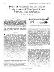
Introduction
3

• High-Rate High-Speed Forward Error Correction
Architectures for Aeronautical Telemetry (HFEC)
»ITTC – University of Kansas
»2-year project
»Sponsored by the Test Resource Management Center
(TRMC) T&E/S&T Program
»FEC decoder prototypes
•SOQPSK-TG modulation
»LDPC
»SCCC
•Other modulations
HFEC Project
4

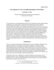
Motivation
• There is a need for a convolutional code SOVA decoder
block written in a hardware description language
»Used multiple places within the HFEC decoder prototypes
»VHDL code can be modified to fit various convolutional codes
with relative ease
• Future students must be able to use the implementation for
the SCCC decoder integration
»Black box
5

• Convolutional Codes
• Channel Models
Background
• Serially Concatenated Convolutional Codes
6

• Class of linear forward error correction (FEC) codes
• Use convolution to encode data sequences
»Encoders are usually binary digital filters
»Coding rate R = k / n
•k input symbols
•n output symbols
Convolutional Codes
• Structure allows for much flexibility
»Convolutional codes operate on streams of data
•Linear block codes assume fixed-length messages
»Lower encoding and decoding complexity than linear block
codes for same coding rates
7

Convolutional Codes
• Convolutional encoders are binary digital filters
»FIR filters are called feedforward encoders
»IIR filters are called feedback encoders
8

Convolutional Codes
• A convolutional encoder can be thought of as a state
machine
»Current memory state and input affect output
»Visualized in a state diagram
9

• Another representation is the trellis diagram
»State diagram shown over time
»Heavily used in many decoding algorithms
•Viterbi algorithm
•Soft output Viterbi algorithm
•Others
Convolutional Codes
K K+ 1
10

• Each stage in the trellis
corresponds to one unit
of time
• Useful labels
»State index: q
•Starting state: q S
•Ending state: q E
»Edge index: e
»Input / output:
m(e) / c(e)
Convolutional Codes
11

Convolutional Codes
• All of the information in a trellis diagram can be contained in
a simple lookup table
»Each edge index corresponds to one row in the table
12

• Convolutional Codes
• Channel Models
Background
• Serially Concatenated Convolutional Codes
13

• Communication links are affected by their environment
»Thermal noise
»Signal reflections
»Similar communication links
Channel Models
• Two common channel models are used when evaluating
the performance of a convolutional code
»Binary symmetric channel (BSC)
»Additive white Gaussian noise channel (AWGN)
14

Channel Models - BSC
• Binary symmetric channel
(BSC)
»Bit is transmitted either correctly
or incorrectly (binary)
•Error occurs with probability p
•Success occurs with probability 1 − p
»Transmission modeled as a
binary addition
•XOR operation
r = s
+
n
15

Channel Models - AWGN
• Additive white Gaussian noise
channel (AWGN)
»Bits are modulated before
transmission (e.g. BPSK)
•s contains values in {−1, +1}
»Noise values are soft (real)
•Gaussian random variables
»Transmission modeled as an
addition of reals
r = s + n
16

• Convolutional Codes
• Channel Models
Background
• Serially Concatenated Convolutional Codes
17

Serially Concatenated Convolutional Codes
• SCCC Encoder
»Two differing convolutional codes are serially concatenated
before transmission
•Separated by an interleaver
•Most previous concatenation schemes involved a convolutional
code and a Reed Solomon code
18

Serially Concatenated Convolutional Codes
• SCCC Decoder
»Two soft-input soft-output (SISO) convolutional decoders
operate on the received sequence
•Separated by an interleaver and de-interleaver
•Multiple iterations before final output (e.g. 10)
19

Serially Concatenated Convolutional Codes
• SCCC Decoder
»Two soft-input soft-output (SISO) convolutional decoders
operate on the received sequence
•Separated by an interleaver and de-interleaver
•Multiple iterations before final output (e.g. 10)
20

Decoding Convolutional Codes
21

Viterbi Algorithm
• Most common algorithm for decoding a convolutionallyencoded
sequence
• Uses maximum likelihood sequence estimation to decode a
noisy sequence
»Uses trellis structure to compare possible encoding paths
»Keeps track of only the paths that occur with maximum
likelihood
• Needs only two* passes over a received sequence to
determine output
»BCJR and Max-Log MAP algorithms need three
»*Can use a windowing technique in the second pass
22

Viterbi Algorithm – Forward Pass
• Path metric updates
»Previous path metrics are added to edge metric increments
»Competing updated metrics are selected based on the
channel model being used
•BSC
•AWGN
• Edge metric increments
»Received symbols compared to edge data
»Resulting increments are added to previous path metrics
• Winning edges
»Two edges merge, one is declared the winner (or survivor)
23

Viterbi Algorithm – Backward Pass
• Also known as the traceback loop
• All known information is processed to determine the
decoded sequence
»Forward pass information
»Trellis lookup table
• For long message lengths, a traceback window can
improve performance
»High probability that all paths converge to a single path some
T time steps back
24

Soft Output Viterbi Algorithm
• Extension of the Viterbi algorithm
• Addition of soft outputs allows it to be more useful in an
SCCC system
»Significant performance gain over use of Viterbi algorithm in
an SCCC decoder
25

Soft Output Viterbi Algorithm
• Same basic calculations as the Viterbi algorithm
• Additional calculations
»Competing path differences
»Path decision reliabilities
»Subtraction of prior probabilities
• Same traceback window applies to the traceback loop
»Includes additional reliability output calculation
26

Soft Output Viterbi Algorithm – Example
0
00
0
01
0
10
0
11
r 0 = {-1, -1}
00
01
10
11
00
01
10
11
• Begin with an empty trellis and like-valued path metrics
27

Soft Output Viterbi Algorithm – Example
0
00
0
01
0
10
1
-1
0
0
-1
1
r 0 = {-1, -1}
00
01
10
00
01
10
0
11
0
0
11
11
• Calculate the edge metric increments for the current trellis
stage (in this case AWGN calculations)
28

Soft Output Viterbi Algorithm – Example
0
00
0
01
0
10
0
11
1
-1
0
0
-1
1
0
0
r 0 = {-1, -1}
1
-1
-1
1
0
0
0
0
00
01
10
11
00
01
10
11
• Add the edge metric increments to their corresponding path
metrics
29

Soft Output Viterbi Algorithm – Example
0
00
0
01
0
10
0
11
1
-1
0
0
-1
1
0
0
r 0 = {-1, -1}
1
Δ 0
(0) = 2
Δ 0
(1) = 2
Δ 0
(2) = 0
Δ 0
(3) = 0
-1
-1
1
0
0
0
0
1
00
1
01
0
10
0
11
00
01
10
11
• Find the absolute difference between competing edges
• Choose the winning metric as the new path metric
30

Soft Output Viterbi Algorithm – Example
0
00
0
01
0
10
0
11
1
-1
0
0
-1
1
0
0
r 0 = {-1, -1}
1
Δ 0
(0) = 2
Δ 0
(1) = 2
Δ 0
(2) = 0
Δ 0
(3) = 0
-1
-1
1
0
0
0
0
1
00
1
01
0
10
0
11
00
01
10
11
• Mark the winning edges
31

Soft Output Viterbi Algorithm – Example
0
00
0
01
0
10
0
11
1
-1
0
0
-1
1
0
0
r 0 = {-1, -1}
1
Δ 0
(0) = 2
Δ 0
(1) = 2
Δ 0
(2) = 0
Δ 0
(3) = 0
-1
-1
1
0
0
0
0
1
00
1
01
0
10
0
11
-1
1
0
0
1
-1
0
0
r 1 = {1, 1}
Δ 1
(0) = 1
Δ 1
(1) = 3
Δ 1
(2) = 1
Δ 1
(3) = 1
0
1
2
-1
1
0
1
0
1
00
2
01
1
10
1
11
• The trellis after two time steps
32

Soft Output Viterbi Algorithm – Example
0/00
1/11
2
0/01
1/10
1/10
2
3
5
• The traceback loop processes the trellis, starting with the
maximum likelihood path metric
• Reliabilities are calculated using the values of Δ that were
found during the forward pass
• Outputs are calculated
33

Hardware Implementation
34

Hardware Implementation
• Designed to work with a systematic rate R = ½ code
»Systematic – message sequence appears within the encoded
sequence
• Design decisions
»Traceback is done with register exchange
»Overflow is prevented by clipping values at a maximum and
minimum
»Path metrics are periodically reduced to prevent them from
becoming too large
»Two global design variables
•Bit width: B
•Traceback length: T
35

Hardware Implementation
• Divided into four blocks
»Metric Manager (MM)
»Hard Decision Traceback Unit (HTU)
»Reliability Traceback Unit (RTU)
»Output Calculator (OC)
36

Hardware Implementation
• Metric Manager
»Handles storage and calculation of path metrics
»Determines winning edges
»Finds absolute path metric differences
37

Hardware Implementation
• Hard Decision Traceback Unit
»Keeps track of hard decision outputs
»Outputs hard decision comparison
•Used by reliability update process
38

Hardware Implementation
• Reliability Traceback Unit
»Keeps track of reliabilities
»Updates each reliability for every clock cycle
39

Hardware Implementation
• Output Calculator
»Determines final output of the decoder
40

Performance Results
41

Performance Results – Software Comparison
• The VHDL decoder was compared with a reference
decoder written in Matlab
»Matlab version known to be correct
• Simulations run for varying SNRs and traceback lengths
»Noise values generated in Matlab
»VHDL decoder simulated in ModelSim using Matlab data
• Simulation requirements
»Transmitted information bits ≥ 1,000,000
»Information bit errors ≥ 100
42

Performance Results – Software Comparison
B = 6
B = 7
B = 8
B = 9
• Traceback length T = 8
43

Performance Results – Software Comparison
B = 6 B = 7
B = 8 B = 9
• Traceback length T = 16
44

Performance Results – Software Comparison
• VHDL implementation approaches Matlab implementation
as B increases
»Expected result – higher precision
• Increase in BER performance as traceback length
increases
»Also expected – designer must determine which traceback
length provides “good enough” performance
45

Performance Results – Hardware
T = 8
T = 16
• VHDL synthesized using Xilinx ISE for the XC5VLX110T
FPGA
»All builds use < 12% of the slices available
»Maximum clock speeds are fast enough to be used in the
SCCC decoder
46

Conclusions and Future Work
47

Summary of Results
• The hardware implementation successfully performs the
soft output Viterbi algorithm
• For all bit widths tested, VHDL curve differs from Matlab
curve by < 1 dB
»For B = 8, difference is < 0.08 dB
• Performance increases as traceback length increases
»Tradeoff between hardware size and decoder precision
• Post-synthesis results
»Small – all designs < 12% slice utilization
»Fast – clock speeds all > 129 MHz
48

Future Work
• New method of overflow prevention
»Current design “clips” values, restricting them to fall within a
certain range
»Work can be done to maintain precision
• FPGA optimization
»Current design approach is very much software-based
»Future designs can take advantage of FPGA features
•Size and speed can be further improved
• Generalized trellis
»Current design focuses on a particular trellis
»Trellis-defining inputs could offer more flexibility
49

Questions?
50