Answer Key Sample 2 1) a) Histogram for Salary Histogram for Age ...
Answer Key Sample 2 1) a) Histogram for Salary Histogram for Age ...
Answer Key Sample 2 1) a) Histogram for Salary Histogram for Age ...

Create successful ePaper yourself
Turn your PDF publications into a flip-book with our unique Google optimized e-Paper software.
<strong>Answer</strong> <strong>Key</strong><br />
<strong>Sample</strong> 2<br />
1)<br />
a)<br />
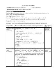
<strong>Histogram</strong> <strong>for</strong> <strong>Salary</strong><br />
Frequency<br />
25<br />
20<br />
15<br />
10<br />
5<br />
0<br />
160 300 440 580 720 860 1000 More<br />
<strong>Histogram</strong> <strong>for</strong> <strong>Age</strong><br />
Frequency<br />
20<br />
15<br />
10<br />
5<br />
0<br />
40 45 50 55 60 65 70 More<br />
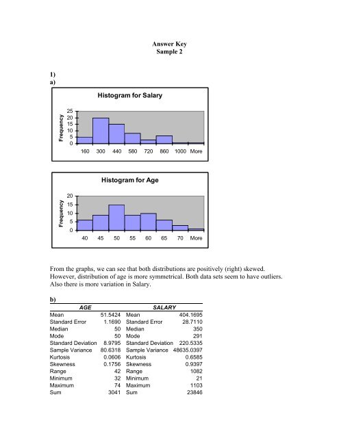
From the graphs, we can see that both distributions are positively (right) skewed.<br />
However, distribution of age is more symmetrical. Both data sets seem to have outliers.<br />
Also there is more variation in <strong>Salary</strong>.<br />
b)<br />
AGE<br />
SALARY<br />
Mean 51.5424 Mean 404.1695<br />
Standard Error 1.1690 Standard Error 28.7110<br />
Median 50 Median 350<br />
Mode 50 Mode 291<br />
Standard Deviation 8.9795 Standard Deviation 220.5335<br />
<strong>Sample</strong> Variance 80.6318 <strong>Sample</strong> Variance 48635.0397<br />
Kurtosis 0.0606 Kurtosis 0.6585<br />
Skewness 0.1756 Skewness 0.9397<br />
Range 42 Range 1082<br />
Minimum 32 Minimum 21<br />
Maximum 74 Maximum 1103<br />
Sum 3041 Sum 23846
Count 59 Count 59<br />
There is more skewness in “<strong>Salary</strong>”. “<strong>Age</strong>” is more symmetrical, mean is equal to median<br />
<strong>for</strong> age. Also by comparing coefficient of variation we can see that there is more<br />
dispersion in “<strong>Salary</strong>”. Also “<strong>Salary</strong>” has small and large outliers.<br />
c) Best measure of center <strong>for</strong> salary is the median, because mean is inflated by large<br />
outliers. Median is better than mean, because it is not sensitive to outliers.<br />
d)<br />
AGE SAL<br />
AGE 79.26515<br />
SAL 248.3149 47810.72<br />
Covariance is 248.3149. This shows that both variables move or covary in the same direction.<br />
We can also say that there is a positive relationship or positive correlation between these two<br />
variables.<br />
e)<br />
Lower Upper Frequency, Midpoint,<br />
Limit Limit fi Xi fi*Xi Xi-mu (Xi-mu)^2 fi*(Xi-mu)^2<br />
20 160 5 90 450 -306.1017 93698.2476 468491.2381<br />
160 300 20 230 4600 -166.1017 27589.7731 551795.4611<br />
300 440 15 370 5550 -26.1017 681.2985 10219.4772<br />
440 580 8 510 4080 113.8983 12972.8239 103782.5912<br />
580 720 3 650 1950 253.8983 64464.3493 193393.0480<br />
720 860 6 790 4740 393.8983 155155.8747 930935.2485<br />
860 1000 1 930 930 533.8983 285047.4002 285047.4002<br />
1000 1140 1 1070 1070 673.8983 454138.9256 454138.9256<br />
Total 59 23370 2997803.3898<br />
mean= 396.1017 Var= 51686.2269 (=2997803.39/58)<br />
23370/59 Std. Dev.= 225.4112<br />
Mean = 396.1017<br />
Median class is one where the (59+1)/2= 30 th observation lives. If we look at the<br />
frequency column, 30 th observation lies within the class 300-440. So this is the median<br />
class.<br />
Modal class is the one with the highest frequency, i.e., 160-300.<br />
f) Standard deviation is 225.4112 (See above)<br />
We applied the <strong>for</strong>mula <strong>for</strong> standard deviation of the grouped data.
2)<br />
a)<br />
Since there are 3 possible answers <strong>for</strong> each question, the probability of guessing an<br />
answer correctly is 1/3, i.e, π=1/3.<br />
=binomdist(10,20,1/3,0) = 0.054<br />
b)<br />
At least 20*(60/100)= 12 questions should be answered correctly to solve the exam. We<br />
are looking <strong>for</strong> the probability that the student guesses 12 or more questions correctly.<br />
=1-binomdist(11,20,1/3,1)<br />
c) 20*(25/100)=5<br />
=1-binomdist(4,20,1/3,1)=0.848<br />
d)<br />
=binomdist(10,20,1/3,1) = 0.962 or<br />
=1-binomdist(9,20,2/3,1)=0.962<br />
e)<br />
E(X)=n⋅π=20⋅(1/3)=6.667<br />
Var(X)=n⋅π⋅(1-π) = 20⋅(1/3)⋅(1-1/3)=4.444<br />
Std.Dev.=sqrt(variance)=2.108<br />
3)<br />
a)<br />
Ability in Mathematics<br />
Interest in Finance Low Average High Total<br />
Low 60 15 20 95<br />
Average 15 35 10 60<br />
High 10 10 25 45<br />
Total 85 60 55 200<br />
b) 45/200<br />
c) We use the following rule<br />
P(A or B)= P(A)+P(B)-P(A and B)<br />
60/200+60/200-35/200=85/200
d) We just look at the “Average Ability in Mathematics” column.<br />
(15+10)/60<br />
e) We look at “Average and High Ability in Mathematics” columns.<br />
(15+20)/(60+55)=35/115