2. Data Import

2. Data Import
The following table displays the different types of input data required for Petrel
along with their formats and types.
Data Format Type
1- Well Data
A- Well Headers Well heads (*.*) Well
B- Well Deviations Well Path deviation (ASCII) (*.*) Well
C- Well Logs Well Log (LAS 3.0) (*.las) Well
2- Well Tops ASCII (*.*) Well Tops
3- 3D Seismic Data Siseworks Horizon Pick (ASCII) (*.*) Lines
4- Fault Data
A- Fault Polygons Zmap+ lines (ASCII) (*.*) Lines
B- Fault Sticks Zmap+ lines (ASCII) (*.*) Lines
5- Isochore Data Zmap+ grid (ASCII) (*.*) Surface
2.1 Well Data
Well data includes three categories of data as will be discussed next.
2.1.1 Well Headers (Well Location Map)
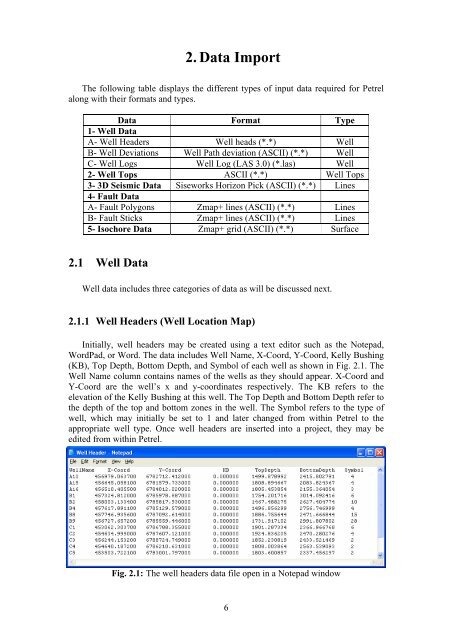
Initially, well headers may be created using a text editor such as the Notepad,
WordPad, or Word. The data includes Well Name, X-Coord, Y-Coord, Kelly Bushing
(KB), Top Depth, Bottom Depth, and Symbol of each well as shown in Fig. 2.1. The
Well Name column contains names of the wells as they should appear. X-Coord and
Y-Coord are the well’s x and y-coordinates respectively. The KB refers to the
elevation of the Kelly Bushing at this well. The Top Depth and Bottom Depth refer to
the depth of the top and bottom zones in the well. The Symbol refers to the type of
well, which may initially be set to 1 and later changed from within Petrel to the
appropriate well type. Once well headers are inserted into a project, they may be
edited from within Petrel.
Fig. 2.1: The well headers data file open in a Notepad window
6

To insert well headers to the project, click the Insert menu command and choose
New Well Folder. A new Wells folder will be added, which will appear in the Project
Explorer Window as a tree view item. Right-click on this item, then select Import (on
Selection)…. The Import File form appears as shown in Fig. 2.2.
Fig. 2.2: The Import File form
Select Well heads (*.*) from the Files of type combo box, specify location and
name of the well headers data file, and press the Open button. The Import Well
Heads form appears as shown in Fig. 2.3. In this step, columns of the well headers
file are identified. When you press OK, the wells are added to the Wells folder.
Fig. 2.3: The Import Well Heads form
7

To display the wells in a 3D window, make sure that a 3D window is active. The
check to the left of the Wells folder toggles the display of the wells in the 3D window.
Once you check the Wells folder, the wells will be displayed as vertical sticks in the
3D window as shown in Fig. 2.4. If the wells are not shown in the window, then click
the View All icon from the 3D Buttons toolbar.
Fig. 2.4: The wells displayed in a 3D window
The settings of the wells may be changed by right-clicking on the Wells folder
and selecting Settings… from the dropdown menu. The Settings for Wells form
appears as shown in Fig. 2.5. Make sure that the Style tab is active. On the Path tab,
change the Pipe width to a number different than the default number; say 50, and
press Apply. Watch what happens, the wells pipe width changes. Now change it once
to a higher number and another to a lower number. Every time you change the pipe
width, press the Apply button for the changes to take effect. Now click the Symbols
tab, change the Font size to a number different than the default number; say 200, and
watch what happens, the well name size changes. Similarly, change the Symbol size
to a number different than the default number; say 200, the well symbol size changes.
Now play with it to get yourself familiar to using this functionality in Petrel.
8

Fig. 2.5: The Settings for 'Wells' form
The well symbol may be independently changed for each well. This is done by
expanding the Wells folder and right-clicking on the well whose symbol is to be
changed. Select Settings… from the dropdown menu. On the Info tab, change the
Well symbol as desired.
The view in the display window may be rotated, moved, or zoomed in and out. To
rotate the view, move the mouse cursor on the 3D window while pressing the left
mouse button. To move the view, move the mouse cursor on the 3D window while
holding down the Ctrl key on the keyboard and pressing the left mouse button. To
zoom the view in and out, move the mouse cursor on the 3D window while holding
down the Ctrl+Shift keys on the keyboard and pressing the left mouse button. Pay
special attention to the green and red arrows at the bottom right corner of the 3D
window. The green arrow should be on top of the red one. Again, try to familiarize
yourself to playing with those functionalities because things will get harder as you
proceed.
9

2.1.2 Well Paths (Well Deviations)
The next piece of well data is well deviations. The well deviations are read into
Petrel in a specific format as shown in Fig. 2.6. A deviated well is traced downward
along its path. The well’s path is sliced into a number of points more enough to
represent its deviation. For each point, the following data is needed: MD, X, Y, Z,
TVD, DX, DY, AZIM, INCL, and DLS. The MD refers to the positive value of the
measured depth of each point. The X and Y values are the x and y-coordinates of each
point respectively. The Z refers to the negative value of the depth of each point. TVD
is the true vertical depth of each point. DX is the difference between the X value of
the point and the well’s x-coordinate. Similarly, DY is the difference between the Y
value of the point and the well’s y-coordinate.
Fig. 2.6: The well deviations data file open in a Notepad window
To insert well deviations to the project, right-click on the Wells folder, then select
Import (on Selection)…. The Import File form appears as shown in Fig. 2.2. Select
Well path/deviation (ASCII)(*.*) from the Files of type combo box. In the File
name combo box, type *.dev and press Open for the deviation wells to be listed.
Select all files, and press Open. The Match Filename and Well window appears as
shown in Fig. 2.7. Match Filename and Well Trace names together, if the match is
wrong, select the correct well name in the well trace column from the drop down box
and press OK. In this study, Well_A10 needs to be matched with the well A10. When
the Import Well Path/Deviation window pops up, click the Input data tab. Check
the TVD, X, Y radio button and specify column numbers of the MD, X, Y, and TVD
as shown in Fig. 2.8. Once you press the "Ok For All", the wells with their
deviations are displayed in the 3D Display Window as shown in Fig. 2.9.
10

Fig. 2.7: The Match Filename and Well form
Fig. 2.8: The Import Well Path / Deviation form
11

Fig. 2.9: The wells with their deviations displayed in a 3D window
12

2.1.3 Well Logs
The last piece of well data is well logs. Well logs are read into Petrel in a specific
LAS format (both LAS 2.0/3.0 formats are currently supported) as shown in Fig. 2.10.
Fig. 2.10: The LAS format log file from Petrel displayed in a Notepad window
Well logs are first scanned using scanning software such as NeuraScan, which
scans well logs and saves them in a graphics format; e.g. TIFF format. Next Neuralog
is used to digitize well logs and convert them into a digital form. Log analysis
software such as Interactive Petrophysics is used to interpret the digitized logs.
Quantities such as formation tops, bottoms, thicknesses, shale volumes, lithologies,
porosities, water saturations, etc. are calculated in this process. Logs are then saved in
LAS format to be imported to Petrel.
To insert well logs to the project, right-click on the Wells folder, then select
Import (on Selection)…. The Import File form appears as shown in Fig. 2.2. Select
Well logs (LAS 3.0) (*.las) from the Files of type combo box. In the File name
combo box, type *.las and press Open for the well logs to be listed. Select all files,
and press Open. The Match Filename and Well window appears as shown in Fig.
2.7. Match Filename and Well Trace names together, if the match is wrong, select
the correct well name in the well trace column from the drop down box and press OK.
When the Import well logs window pops up, choose the Property Template of the
log from the Undefined Well Log group box. In this case, choose the Net/Gross
property template to be attached to the NetGross log as shown in Fig. 2.11. When you
press OK For All, the logs associated with each well will be inserted under each
wellbore as well as under the Global well logs folder.
13

Fig. 2.11: The Import well logs form
Logs may be displayed for all wells or for a specific well. To display logs of all
wells, expand the Global well logs item and select the logs to be displayed for all
wells as shown in Fig. 2.12. To display logs of a certain well, expand the well’s item,
next expand its Well logs item, and finally select the logs to be displayed for that
well. The logs will be attached to the existing well path in a manner similar to the
attachment of the well path to the well header. Fig. 2.12 shows the Fluvialfacies and
Perm logs displayed in a 3D window for all wells.
Fig. 2.12: Fluvialfacies and Perm logs displayed in a 3D window
14

2.2 Well Tops
Initially, well tops data file may be created using a text editor such as the Notepad,
WordPad, or Word. The well tops data includes: X, Y, Depth, Time, Type, Horizon
Name, Well Name, Symbol, Measured Depth, Pick Name, Interpreter, Dip Angle, and
Dip Azimuth of each well as shown in Fig. 2.13.
Fig. 2.13: Well tops data file open in a Notepad window
The X and Y are the well’s x and y-coordinates respectively. The Depth and Time
refer to the horizon's depth and time. The Type refers to the type of the stratigraphic
sequence (Horizon, Zone, and Layer). Horizon Name and Well Name refer to the
horizon and well names respectively. The Symbol refers to the type of well, which
may initially be set to 1 and later changed to the appropriate well type from within
Petrel. Measured Depth refers to the measured depth of the horizon name.
To insert well tops to the project, click the Insert menu command and choose
New Well Tops. A new Well Tops folder will be added, which will appear in the
Project Explorer Window as a tree view item. Right-click on this item, then select
Import (on Selection)…. The Import File form appears as shown in Fig. 2.2. Select
Petrel Well Tops (ASCII) (*.*) from the Files of type combo box. Specify location
and name of the well tops data file and press the Open button. The Import Petrel
Well Tops: Well Tops appears as shown in Fig. 2.14. Press Ok For All and then
press OK to close the information window.
Now, as an exercise, hide the well logs and display well tops. Well tops might not
be shown clearly; you may need to change the settings of the well tops as you did
before in the well headers. Again, try to familiarize yourself to playing with other
factors because things will get harder as you proceed. If you set the settings for well
tops correctly, you are supposed to get something like Fig. 2.15 for well tops.
15

Fig. 2.14: The Import Petrel Well Tops: Well tops form
Fig. 2.15: Well tops displayed in a 3D window
16

2.3 3D Seismic Lines
The 3D seismic lines are read into Petrel in a specific Seisworks horizon picks
format as shown in Fig. 2.16.
Fig. 2.16: The 3D seismic lines for Top Tarbert open in a Notepad window
The 3D seismic lines may be obtained via software like KingdomSuite package,
which converts a surface into a digital form. Next surface analysis software is used to
interpret the digitized seismic data. Surfaces are then saved in the Seisworks horizon
picks format to be imported to Petrel.
To insert the seismic lines to the project, click the Insert menu command and
choose New Interpretation Folder. A new interpretation folder will be added, which
will appear in the Project Explorer Window as a tree view item. Right-click on this
item, then select Import (on Selection)…. The Import File form appears as shown in
Fig. 2.2. Select Seisworks horizon picks (ASCII) (*.*) format from the Files of type
combo box. Specify location and name of the seismic data files to be inserted into the
project. In this case, select the Seismic Interpretation (time) in the Look in combo
box, then select all files and press the Open button. The Input data dialog form
appears. Make sure that the correct domain is selected, in this case, the Elevation
Time option should be selected from the Domain combo box, as shown in Fig. 2.17,
and press the Ok For All button.
Fig. 2.17: The Input data dialog
17

To display the seismic surfaces, expand the interpretation folder by clicking the
plus sign to its left, then select the surfaces to be displayed as shown in Fig. 2.18.
Fig. 2.18: Seismic data of Top Tarbert, Top Ness, and Top Etive, displayed in a 3D
window
Now spend some time playing with the settings of each set of data. For example,
deselect the wells, well tops, and seismic data, and only select the Top Tarbert
seismic surface. Then display its settings dialog as shown in Fig. 2.19.
Fig. 2.19: Settings for 'Top Tarbert'
18

2.4 Fault Data
Fault data is entered to Petrel in one of two forms; either fault polygons or fault
sticks as follows:
2.4.1 Fault Polygons
Fault polygons may be created from within Petrel. Their files can be edited with
any text editor such as Notepad as shown in Fig. 2.20.
Fig. 2.20: The Tarbert fault polygons data file open in a Notepad window
To insert fault polygons to the project, click the Insert menu command and
choose New Folder. A New folder will be added, which will appear in the Project
Explorer Window as a tree view item. Rename the folder to Fault Polygons by right
clicking on the folder and select Settings… from the dropdown menu. On the
Settings dialog box, change the name and press OK. Now right-click on the Fault
Polygons folder, then select Import (on Selection)…. The Import File form appears
as shown in Fig. 2.2. Select Zmap+ lines (ASCII) (*.*) from the Files of type combo
box. Specify location and name of the fault polygons data files and press the Open
button. In this case, select the Fault Polygons (time) in the Look in combo box, then
select all files and press the Open button. The Input data dialog form appears as
shown in Fig. 2.21. Make sure that the correct domain and line type are selected; in
this case, the Elevation Time option and the Fault polygons should be selected from
the Domain and Line Type combo boxes. Press the Ok For All button.
Fig. 2.21: The Input data dialog
19

To display the fault polygons, expand the Fault Polygons folder by clicking the
plus sign to its left, then select the fault polygons to be displayed as shown in Fig.
2.22.
Fig. 2.22: The fault polygons of Tarbert, Ness, and Etive, displayed in a 3D window
At this stage, you should spend some time playing with different settings and
options to familiarize your self to Petrel.
20

2.4.2 Fault Sticks
Fault sticks may be created from within Petrel. Their files can be edited with any
text editor such as Notepad as shown in Fig. 2.23.
Fig. 2.23: The fault sticks data file open in a Notepad window
To insert fault sticks to the project, click the Insert menu command and choose
New Folder. A New folder will be added, which will appear in the Project Explorer
Window as a tree view item. Rename the folder to Fault Sticks by right-clicking on
the folder and select Settings… from the dropdown menu. On the Settings dialog,
change the name and press OK. Now right-click on the Fault Sticks folder, then
select Import (on Selection)…. The Import File form appears as shown in Fig. 2.2.
Select Zmap+ lines (ASCII) (*.*) from the Files of type combo box. Specify
location and name of the fault polygons data files and press the Open button. In this
case, select the Fault Sticks (time) in the Look in combo box, then select For Create
From FS folder, then select all files and press the Open button. The Input data
dialog form appears. Make sure that the correct domain and line type are selected; in
this case, the Elevation Time option and the Fault sticks should be selected from the
Domain and Line Type combo boxes, as shown in Fig. 2.24, and press the Ok For
All button. Repeat the same process for other fault sticks folders to be inserted into
the project.
Fig. 2.24: The Input data dialog
21

To display the fault sticks, expand the Fault Sticks folder by clicking the plus
sign to its left, then select the fault sticks to be displayed as shown in Fig. 2.25.
Fig. 2.25: The fault sticks displayed in a 3D window
2.5 Isochore Data
The isochore data is read into Petrel in a specific Zmap+ grid format as shown in
Fig. 2.26.
Fig. 2.26: The isochore data file open in a Notepad window
22

To insert isochore data to the project, click the Insert menu command and choose
New Folder. A New folder will be added which will appear in the Project Explorer
Window as a tree view item. Rename the folder to Isochores by right-clicking on the
folder and select Settings… from the dropdown menu. On the Settings dialog box,
change the name and press OK. Now right-click on the Isochores folder, then select
Import (on Selection)…. The Import File form appears as shown in Fig. 2.2. Select
Zmap+ grid (ASCII) (*.*) from the Files of type combo box. Specify location and
name of the isochore data files and press the Open button. In this case, select the
Isochores (depth) in the Look in combo box, then select the Ness folder, then select
all files and press the Open button. The Input data dialog form appears. Make sure
that the correct template is selected, in this case, the Thickness Depth option should
be selected from the Template combo box as shown in Fig. 2.27, and press the Ok
For All button. Repeat the same process for the Tarbert folder to be inserted into the
project. To display the isochore data, expand the Isochores folder by clicking the plus
sign to its left, then select the isochores to be displayed as shown in Fig. 2.28.
Fig. 2.27: The Input data dialog
With this step, most of the required data were input to Petrel. A chart of the input
data with their formats, types, categories, and domains is shown in Fig. 2.29. Next,
some editing of the input data is necessary before we start building the 3D geological
model of the petroleum reservoir. Editing of the input data will be discussed in the
next section.
23

Fig. 2.28: The Ness 1 isochores displayed in a 3D window
Data
Formats
Type
Category
Domain
Wells
Wellhead-deviation-logs
Well
Depth
Well tops
Petrel Well Tops
Well tops
Depth
3D seismic lines
Seisworks Horizon Picks
Lines
Horizon
Time
Fault polygons
ZMAP+ lines (ASCII)
Lines
Fault polygons
Time
Fault sticks
ZMAP+ lines (ASCII)
Lines
Fault sticks
Time
Surfaces (Time)
Zmap+ grid
Surface
Elevation
Time
Isochores (Depth)
Zmap+ grid
Surface
Thickness
Depth
Properties
Zmap+ grid
Surface
Property
Respective
Template
Velocity Data
Zmap+ grid
Surface
Property
Velocity
Template
Extra data
Formats
Category
Unit
Seismic cube / 2D
SEG-Y
Seismic
Seismic
Template
Images
Bitmap (bmp, jpeg....)
No
No
No
Summary Files
Petrel summary data ASCII
Eclipse grid
Fig. 2.29: Petrel data types with their formats, categories, and domains
24

2.6 Import Data from Another Project
Any type of data can be copied between projects. This functionality allows for
having a master project containing regional data. Parts of this data can then be copied
over to a new project for detailed analysis of parts of the area. In this exercise you will
import all the remaining data required for the following exercises by copying them
from an existing project.
To import data from another project, follow the steps:
• Select File> Open Secondary Project.
• Select the Input_Data.pet file found under the Project folder. See Fig. 2.30.
• Drag and drop all the Input flies that you are missing into the Input tab of your
project.
Fig. 2.30: The Input_Data.pet (read-only) displayed in a 3D window
2.7 Quality Check (QC) of Imported Data
After data has been imported into Petrel, you should always do a quality control and
check if they look as you expected them to do. Typical ways of QC data are to display
them and also to check the statistics. Using the general intersection to view the data in
cross section and playing through the data set is a powerful tool as well. As an
example, when you do the quality check of the fault polygons you have imported, you
will see that they don’t have any Z value. This we are going to fix in the next chapter
with the editing of the input data.
25