February 13

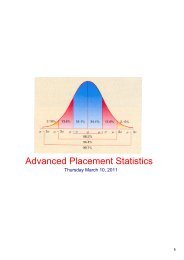
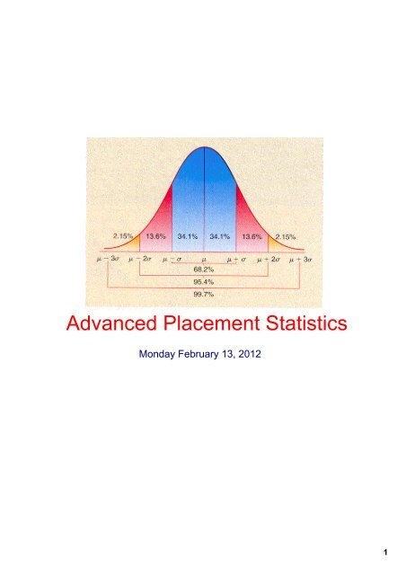
Advanced Placement Statistics
Monday February 13, 2012
1

Daily Agenda
1. Welcome to class
2. Please find folder and take
your seat.
3. Review Chapter 10 Section 1 worksheet
4. Introduce Chapter 10 Section 2
5. Practice finding upper critical t values
6. Explain matched pairs inference
7. Collect Folders
2

HOMEWORK REVIEW
3

10.24 Newts and the data distribution
conclusion ­ no outliers, small skew
4

OTL C10#4
P 632: 10.12,
P 637: 10.14, and 10.17
5

10.14 pg 637
To assess the accuracy of a laboratory scale, a standard
weight known to weigh 10 grams is weighed repeatedly.
The scale readings are Normally distributed with unknown
mean (the mean is 10 g if the scale has no bias). The
standard deviation of the scale readings is known to be
0.0002 gram.
a) The weight is weighed five times. The mean result is
10.0023 grams. Construct and interpret a 95% confidence
interval for the mean of repeated measurements of the
weight.
P
μ = the mean of repeated measurements of this standard weight
A
∎ We must assume that the sample is random,
so x is an unbiased estimator of μ.
∎ we are told that our sample is taken from a normal
population, so the shape of the sampling distribution is
approximately normal.
N
∎ 10(5) = 50 and assume 50 < total number of times we could repeatedly
weigh the weight , so is appropriate for the sampling
distribution standard deviation.
Use a z ­ confidence interval for a population mean
I 10.0023 ± 1.96 (0.0002/√5 )
C I am 95% confident that the true mean scale reading for a 10
gram weight is captured by the interval (10.0021, 10.0025)
grams.
8

10.14 pg 637
To assess the accuracy of a laboratory scale, a standard
weight known to weigh 10 grams is weighed repeatedly.
The scale readings are Normally distributed with unknown
mean (the mean is 10 g if the scale has no bias). The
standard deviation of the scale readings is known to be
0.0002 gram.
b) How many measurements must be averaged together
to get a margin of error of ± 0.0001 with 98% confidence?
9

10.17 pg 638
A radio talk show invites listeners to enter a dispute about a
proposed pay increase for city council members. "What
yearly pay do you think council members should get? Call
us with your number." In all, 958 people call. The mean
pay they suggest is x = $8740 per year, and the standard
deviation of the responses is s = $1125. For a large sample
such as this, s is very close to the unknown population σ.
The station calculates the 95% confidence interval for the
mean pay μ that all citizens would propose for council
members to be $8669 to $8811.
a) Is the station's calculation correct ?
b) Does their conclusion describe the population of all the city's citizens?
Explain your answer.
10

OTL C10#5
P 640: 10.19, 10.20 b only
P 641: 10.21, 10.22, 10.25
10.19 a) sentence(s) three conditions
b) just the I part of PANIC
c) sentence (our special one)
10.20 b) only show your arithmetic
10.21 Sentence to answer question.
10.22 Sentence to justify answer.
10.25 Use 10.24 for the numbers.
show your arithmetic
11

CONFIDENCE
INTERVAL
CAUTIONS
!
!
!
Inference must assume SRS
Always round up when finding n
The size of the sample determines
the margin of error NOT the size of
the population
16

CONFIDENCE INTERVAL
CAUTIONS
!
!
Different methods are needed for
different sampling designs
There is no correct method for
inference from BAD data (bias,
poorly collected, no known sample
size)
! Outliers can distort the results
!
!
The shape of the population
distribution matters (condition 2)
FOR z we must know σ
17

The "parent" or original normal curve function.
18

Area under the standard normal curve = 1
19

Let's Get REAL ­­ no σ
What happens when we are in the real world and
we don't have any secret messages from above.
We DO NOT know the population standard
deviation σ. SO what do we do?
What to do ???
Use S x instead ----⇒ what are the consequences ?
Obviously more room for error ...
20

Goal ­ Calculate and interpret a confidence Interval
Part 1 - calculate an upper critical t score (t*)
1. Sketch a semi - normal curve (floating), add the
confidence level into the curve
2. Subtract to find the area
outside the confidence level.
3. Add to find the area to the left of
the desired t score (t * ). This is
called the upper critical t score
4. Look up the t score for the given area.
This is a backwards table problem
OR use the t-AREA (add degrees of freedom)
program in your calculator. This is the desired t *
23

Goal ­ Calculate and interpret a confidence Interval
Part 2 - calculate the confidence interval
USE THE PANIC METHOD
P ­ parameter declaration or description
A ­ assumptions (check the assumption)
N ­ name the test that your will use
I ­ interval, calculate the confidence interval (math)
C ­ conclusion, state your conclusion using our sentence
25

MORE DETAIL of PANIC
P ­ μ = the mean of the population
ρ = the population proportion
make this description very specific to the problem
A ­ assumptions (3 to check)
1) SRS must be stated in the problem
2) check for "normality"
a) this can be stated in the problem
b)
**
* Sample size < 15.
NO OUTLIERS, NORMAL POPULATION
* Sample size ≥ 15.
NO OUTLIERS, NO STRONG SKEW
* Large sample size (n > 30)
NO OUTLIERS
if n(p) ≥ 10 and n(p­1)≥10
∧
then thumb 2 passes for ρ,p world
c) plot a histogram or boxplot and eyeball
the graph for "normality"
3) 10(n) ≤ total population
(Independence and thumb 1)
(no better method available)
N ­ name the test
t­ confidence interval for a population mean
with _____ degrees of freedom
I ­ Interval (do the math)
C ­ conclusion
I am ____% confident that the true (mean or
proportion) of the ________ population is
captured by the interval ( , ) units.
make this description very specific to the problem
26

** Using the t proceedures CAUTIONS
* except in the case of small samples, the assumption that
the data are from an SRS is more important than the
assumption that the population distribution is normal
* Sample size < 15.
NO OUTLIERS, NORMAL POPULATION
* Sample size ≥ 15.
NO OUTLIERS, NO STRONG SKEW
* Large sample size (n > 30)
NO OUTLIERS
29

PRACTICE page 648: 10.27, 10.31
10.27 a) find the standard error of the mean
1.789785834
b) 0.84±0.01 and n = 3
SEM = ?
34

10.31 Give it some gas!
35

10.31 Give it some gas!
36

t-curve explanation and exploration
10.37 finding t using a table
37

Matched Paired t Procedures
The parameter μ in paired t procedure is ...
∎ the mean difference in the responses to the two treatments
within matched pairs of subjects in the entire population
∎ the mean difference in response to the two treatments for
individuals in the population (when the same subject
receives both treatments)
∎ the mean difference between before-and-after
measurements for all individuals in the population.
39

Class examples page 657 & 658 10.33, 10.35, 10.36
40

AP STATISTICS HOMEWORK ASSIGNMENT due 2/14/12
page 649: 10.30 list CSB
page 650: 10.32 list AMBER
page 659: 10.39 and 10.40
list HAV
41

What type of plot is this?
How do you analyze this plot?
51