2012 - Krell Institute

More documents

Recommendations

Info

alumni profiles Richard Katz University of Oxford Delving into the Deep Earth rarea wasn’t a particularly deep decision at the time. RICHARD KATZ may spend his time contemplating what happens far below Earth’s surface now, but his choice of research “There was never a moment when I said, ‘This is what I’m interested in studying – geophysics of the deep Earth,’” says Katz, a Department of Energy Computational Science Graduate Fellowship (DOE CSGF) recipient from 2001 to 2005. “It was an evolution over probably my whole life. Small decisions led me to where I am.” Here’s where Katz is: a lecturer in the Department of Earth Science at England’s University of Oxford. He uses computers to model processes occurring deep in the Earth, like plate tectonics, mantle convection and the phase changes that drive magma creation and movement. The models are used to make measurable predictions. The challenge for deep-Earth researchers, Katz says, “is to connect the processes that are happening in places beyond our ability to observe with the consequences of those processes, which are accessible” to measurement and quantification. A volcano, for example, is an observable manifestation of processes happening far below ground. In a recent project, Katz and his colleagues studied how the heterogeneous nature of Earth’s mantle – the rocky layer between the crust and the molten core – affects magma genesis and migration. As crustal rocks are pushed deep below the surface into the convecting mantle “it’s like a taffy pull,” Katz says. “You have stripes and blobs of different composition and those different compositions have different melting properties,” complicating magma’s movement below the surface. In a paper published online in the journal Earth and Planetary Science Letters, Katz and doctoral student Samuel Weatherley modeled magma-mantle dynamics and melting reactions beneath mid-ocean ridges. The model says that when mantle heterogeneities melt preferentially, the magma creates isolated channels that provide a path for rapid ascension toward the surface. That flow may be how magma moves, in isolation from the surrounding mantle, to the boundary between the crust and the mantle along the mid-ocean ridges. The model also suggests that pools of magma get trapped at the boundary of Earth’s solid outer layers. The pools feed volcanoes or solidify, making the mantle more heterogeneous. Katz and his research group use similar techniques to model structures near the other temperature extreme: ice sheets and glaciers. Ice and subsurface materials share many of the same P22 DEIXIS 12 DOE CSGF ANNUAL
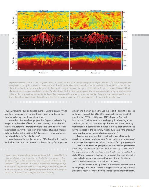
Representative output from two ridge simulations. Panels (a) and (d) show the compositional perturbation of solidus temperature as a physical proxy for chemical heterogeneity. The boundary between partially molten and unmolten mantle is marked in black. Panels (b) and (e) show the porosity field with a log-scale color bar; porosities below 0.1 percent are shown as black. Mantle streamlines are overlain in white. Panels (c) and (f) show the mantle potential temperature, with a color scale chosen to highlight temperature variability in the asthenosphere – the upper layer of the mantle. Temperature contours within the lithosphere (the layer above the asthenosphere) are overlain in white. The grid spacing is 1 km in both simulations. physics, including flows and phase changes under pressure. While scientists recognize the role ice shelves have in Earth’s climate, there’s much they don’t know about them. In another climate-related project, Katz’s group is developing computational models of how “volatiles” – water, carbon dioxide and other substances – transfer from the solid Earth to the oceans and atmosphere. “In the long term, over millions of years, climate is really controlled by the solid Earth,” Katz adds. “The atmosphere is the tail and the solid Earth is the dog.” Katz develops his calculations with PETSc (Portable, Extensible Toolkit for Scientific Computation), a software library for large-scale These images show melting rate and magmatic flow speed for two ridge simulations. The simulation on the far left was begun with a random array of fertile blobs while the simulation on the near left was begun with a smoothed, random-noise field. Panels (a) and (c) show the melting rate in units of 10 -3 kg/m 3 /year. Panels (b) and (d) show the magnitude of magma velocity in units of meters per year. Note that the color scale is logarithmic in the velocity. simulations. He first learned to use this toolkit – and other science software – through the DOE CSGF, especially during his 2003 practicum at PETSc’s birthplace, DOE’s Argonne National Laboratory. “I’m interested in spending my time learning about the Earth, so the fact I can leverage these sophisticated tools by world leaders in computation means I can solve problems without having to create all the machinery myself,” Katz says. “The practicum was a key step in my thesis and subsequent work.” Another key step was Katz’s National Science Foundation postdoctoral research fellowship at Oxford’s rival, the University of Cambridge. The experience helped lead to his faculty appointment. Katz calls his research group FoaLab to honor his grandfather, Piero Foa, an endocrinologist who fled fascist Italy for the United States, where he made key discoveries about Type I diabetes. Foa stoked his grandson’s curiosity, sharing everything from dissecting frogs to building sand volcanoes. Foa was 94 when he died in 2005, shortly before Katz received his doctorate. “I think he would be happy to see me working in a field that’s at the cutting edge,” Katz adds. The use of large-scale computing to study problems in nature is “one of the ways science is advancing most rapidly.” DEIXIS 12 DOE CSGF ANNUAL P23
Page 1 and 2: DEPARTMENT OF ENERGY COMPUTATIONAL
Page 3 and 4: TABLE OF CONTENTS 20 22 26 4 Practi
Page 5 and 6: MMER INTERNSHIP The Department of E
Page 7 and 8: would be to scale up to rapidly ass
Page 9 and 10: FELLOW PROBES PROBABILITY IN QUANTI
Page 11 and 12: Top right: Comparison of Kriging er
Page 13 and 14: MOVIE CHALLENGE SPARKS PRACTICUM -
Page 15 and 16: The components capture email conver
Page 17 and 18: SAMPLING SURROGATES TO WEIGH UNCERT
Page 19 and 20: Left: This graph compares BMARS pre
Page 21: E GLOBE ckey Pucks focus computatio
Page 25 and 26: of exposure is safe for a chemical.
Page 27 and 28: The sun contributes approximately 1
Page 29 and 30: forever. But most remained, and aft
Page 31 and 32: ABOUT FRED HOWES undergraduate and
Page 33 and 34: TH YEAR FELLOWS RD YEAR FELLOWS Edw
Page 35 and 36: ST YEAR FELLOWS Samuel Blau Harvard
Page 37 and 38: Edward Chao Princeton University Co
Page 39 and 40: Noel Gres University of Illinois at
Page 41 and 42: Brian Moore North Carolina State Un
Page 43 and 44: Obioma Uche Princeton University Mo

2012 - Krell Institute

Create successful ePaper yourself

Delete template?

Save as template?