Numerical Geometric Integration Ernst Hairer

Numerical
Geometric Integration
Ernst Hairer
Universite de Geneve March 1999
Section de mathematiques
Case postale 240
CH-1211 Geneve 24

Contents
I Examples and Numerical Experiments 1
I.1 Two-Dimensional Problems . . . . . . . . . . . . . . . . . . . . . . . . . . 1
I.2 Kepler's Problem and the Outer Solar System . . . . . . . . . . . . . . . 4
I.3 Molecular Dynamics . . . . . . . . . . . . . . . . . . . . . . . . . . . . . 8
I.4 Highly Oscillatory Problems . . . . . . . . . . . . . . . . . . . . . . . . . 11
I.5 Exercises . . . . . . . . . . . . . . . . . . . . . . . . . . . . . . . . . . . . 12
II Numerical Integrators 13
II.1 Implicit Runge-Kutta and Collocation Methods . . . . . . . . . . . . . . 13
II.2 Order Conditions, Trees and B-Series . . . . . . . . . . . . . . . . . . . . 17
II.3 Adjoint and Symmetric Methods . . . . . . . . . . . . . . . . . . . . . . . 21
II.4 Partitioned Runge-Kutta Methods . . . . . . . . . . . . . . . . . . . . . . 23
II.5 Nystrom Methods . . . . . . . . . . . . . . . . . . . . . . . . . . . . . . . 27
II.6 Methods Obtained by Composition . . . . . . . . . . . . . . . . . . . . . 27
II.7 Linear Multistep Methods . . . . . . . . . . . . . . . . . . . . . . . . . . 29
II.8 Exercises . . . . . . . . . . . . . . . . . . . . . . . . . . . . . . . . . . . . 29
III Exact Conservation of Invariants 31
III.1 Examples of First Integrals . . . . . . . . . . . . . . . . . . . . . . . . . . 31
III.2 Dierential Equations on Lie Groups . . . . . . . . . . . . . . . . . . . . 34
III.3 Quadratic Invariants . . . . . . . . . . . . . . . . . . . . . . . . . . . . . 36
III.4 Polynomial Invariants . . . . . . . . . . . . . . . . . . . . . . . . . . . . . 38
III.5 Projection Methods . . . . . . . . . . . . . . . . . . . . . . . . . . . . . . 40
III.6 Magnus Series Expansion . . . . . . . . . . . . . . . . . . . . . . . . . . . 43
III.7 Lie Group Methods . . . . . . . . . . . . . . . . . . . . . . . . . . . . . . 46
III.8 Exercises . . . . . . . . . . . . . . . . . . . . . . . . . . . . . . . . . . . . 48
IV Symplectic Integration 51
IV.1 Hamiltonian Systems . . . . . . . . . . . . . . . . . . . . . . . . . . . . . 51
IV.2 Symplectic Transformations . . . . . . . . . . . . . . . . . . . . . . . . . 52
IV.3 Symplectic Runge-Kutta Methods . . . . . . . . . . . . . . . . . . . . . . 56
IV.4 Symplecticity for Linear Problems . . . . . . . . . . . . . . . . . . . . . . 59
IV.5 Campbell-Baker-Hausdor Formula . . . . . . . . . . . . . . . . . . . . . 60
IV.6 Splitting Methods . . . . . . . . . . . . . . . . . . . . . . . . . . . . . . . 62
IV.7 Volume Preservation . . . . . . . . . . . . . . . . . . . . . . . . . . . . . 66
IV.8 Generating Functions . . . . . . . . . . . . . . . . . . . . . . . . . . . . . 66
2

IV.9 Variational Approach . . . . . . . . . . . . . . . . . . . . . . . . . . . . . 66
IV.10 Symplectic Integrators on Manifolds . . . . . . . . . . . . . . . . . . . . . 66
IV.11 Exercises . . . . . . . . . . . . . . . . . . . . . . . . . . . . . . . . . . . . 66
V Backward Error Analysis 68
V.1 Modied Dierential Equation { Examples . . . . . . . . . . . . . . . . . 68
V.2 Structure Preservation . . . . . . . . . . . . . . . . . . . . . . . . . . . . 72
V.2.1 Reversible Problems and Symmetric Methods . . . . . . . . . . . . 72
V.2.2 Hamiltonian Systems and Symplectic Methods . . . . . . . . . . . . 74
V.2.3 Lie Group Methods . . . . . . . . . . . . . . . . . . . . . . . . . . . 75
V.3 Modied Equation Expressed with Trees . . . . . . . . . . . . . . . . . . 75
V.4 Modied Hamiltonian . . . . . . . . . . . . . . . . . . . . . . . . . . . . . 78
V.5 Rigorous Estimates { Local Error . . . . . . . . . . . . . . . . . . . . . . 78
V.5.1 The Analyticity Assumption . . . . . . . . . . . . . . . . . . . . . . 79
V.5.2 Estimation of the Derivatives of the Numerical Solution . . . . . . . 79
V.5.3 Estimation of the Coecients of the Modied Equation . . . . . . . 81
V.5.4 Choice of N and the Estimation of the Local Error . . . . . . . . . 83
V.5.5 Estimates for Methods that are not B-series . . . . . . . . . . . . . 84
V.6 Longtime Error Estimates . . . . . . . . . . . . . . . . . . . . . . . . . . 84
V.7 Variable Step Sizes . . . . . . . . . . . . . . . . . . . . . . . . . . . . . . 87
V.8 Exercises . . . . . . . . . . . . . . . . . . . . . . . . . . . . . . . . . . . . 87
VI Kolmogorov-Arnold-Moser Theory 88
VI.1 Completely Integrable Systems . . . . . . . . . . . . . . . . . . . . . . . . 88
VI.2 KAM Theorem . . . . . . . . . . . . . . . . . . . . . . . . . . . . . . . . 88
VI.3 Linear Error Growth . . . . . . . . . . . . . . . . . . . . . . . . . . . . . 88
VI.4 Exercises . . . . . . . . . . . . . . . . . . . . . . . . . . . . . . . . . . . . 88
Bibliography 89
This manuscript has been prepared for the lectures \Integration geometrique des equations
dierentielles" given at the University of Geneva during the winter semester 1998/99
(2 hours lectures and 1 hour exercises each week). It is directed to students in the third
or fourth year. Therefore, a basic knowledge in Analysis, Numerical Analysis and in the
theory and solution techniques of dierential equations is assumed.
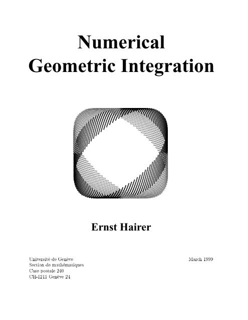
The picture of the title shows parasitic solutions, when the 2-step explicit midpoint
rule is applied to the pendulum problem with step size h = =10:5 (6000 steps), initial
values q(0) = 0, _q(0) = 1, and exact starting values. It is taken from [Hai99].
At this place I wanttothankallmy friends and colleagues, with whom I had discussions
on this topic and who helped me to a deeper understanding of the subject "Numerical Geometric
Integration". In particular, I am grateful to Gerhard Wanner, Christian Lubich,
Sebastian Reich, Stig Faltinsen, David Cohen, Robert Chan, :::, and to Pierre Leone who
assisted me during the lectures.

Preface
The numerical solution of ordinary dierential equations has a long history. The rst and
most simple numerical approachwas described by L. Euler (1768) in his \Institutiones Calculi
Integralis". A.L. Cauchy (1824) established rigorous error bounds for Euler's method
and, for this purpose, employed the implicit -method (for more details see [HNW93,
Sects. I.7, II.1, III.1], [BW96]).
The current most popular methods are Runge-Kutta methods and linear multistep
methods. Runge-Kutta methods have been developed by G. Coriolis (1837), C. Runge
(1895), K. Heun (1900), W. Kutta (1901), and their analysis has been brought to perfection
by J.C. Butcher in the sixties and early seventies. Linear multistep methods have
their origin in the work of J.C. Adams, which was carried out in 1855 and published in the
book of F. Bashforth (1883). The importantwork of G. Dahlquist (1959) unied and completed
the theory for multistep methods. For a comprehensive study of Runge-Kutta as
well as multistep methods we refer the reader to the monographs [Bu87, HNW93, HW96].
The above-mentioned works mainly considered the approximation of one single solution
trajectory of the dierential equation. Later one became aware of the fact that much
new insight can be gained by considering a numerical method as a discrete dynamical
system which approximates the ow of the dierential equation. This point of view has
its origin in the study of symmetric methods (see G. Wanner [Wa73], who used the symbol
m h (y 0 ) for the discrete ow) and is the central theme in the works of Feng Kang, collected
in [FK95], U. Kirchgraber [Ki86], W.-J. Beyn [Be87], T. Eirola [Ei88] and in the mongraphs
of P. Deuhard & F. Bornemann [DB94], J.M. Sanz-Serna & M.P. Calvo [SC94]
and A.M. Stuart & A.R. Humphries [StH96]. One started to study whether geometrical
properties of the ow (such as the preservation of rst integrals, the symplecticity,
reversibility,orvolume-preservation of the ow) can carry over to the numerical discretization.
Such properties are crucial for a qualitatively correct simulation of the dynamical
system. They turn out to be also responsible for a more favourable error propagation in
long-time integrations.
These lecture notes are organized as follows: we start with some examples (related to
realistic problems) and illustrate the dierent qualitativebehaviours of numerical methods
in Chapter I. We then review numerical integrators and focus our attention on collocation,
symmetric and partitioned methods (Chapter II). Geometric properties such as the
conservation of rst integrals (Chapter III) and the symplecticity for Hamiltonian systems
(Chapter IV) are discussed in detail. A main technique for a deeper understanding
of geometric properties of numerical methods is \backward error analysis" which will be
explained in Chapter V. If time permits, we also consider KAM theory (Chapter VI)
as far as it is needed for the explanation of numerical phenomena concerning the longtime
integration of integrable systems. The title of these lecture notes is inuenced by
J.M. Sanz-Serna's survey article [SS97]. We have included the term \numerical" in order
to distinguish it clearly from H. Whitney's \Geometric integration theory".
Geneva, date
Ernst Hairer

Chapter I
Examples and
Numerical Experiments
This chapter introduces some interesting dierential equations and illustrates the dierent
qualitative behaviour of numerical methods. We deliberately consider only very simple
numerical methods of orders 1 and 2 in order to emphasize the qualitative aspects of
the experiments. The same eects (on a dierent scale) could be observed with more
sophisticated higher order integration schemes. The presented experiments should serve
as a motivation for the theoretical and practical investigations of later chapters. Every
reader is encouraged to repeat the experiments or to invent similar ones.
I.1 Two-Dimensional Problems
Volterra-Lotka Problem Consider the problem
u 0 = u(v ; 2) v 0 = v(1 ; u) (1.1)
which constitutes an autonomous system of two dierential equations. It is a simple model
for the development of two populations, where u represents the predator and v the prey.
If we divide the two equations of (1.1) by each other and if we consider u as a function of
v (or reversed), we get after separation of variables
Integration then leads to
1 ; u
u du ; v ; 2 dv =0:
v
I(u v) =lnu ; u +2lnv ; v = Const: (1.2)
This means that solutions of (1.1) lie on level curves of (1.2) or, equivalently, I(u v) isa
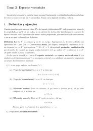
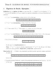
rst integralof(1.1). Some of the level curves are drawn in the pictures of Fig. 1.1. Since
these level curves are closed, all solutions of (1.1) are periodic. Can we have the same
property for the numerical solution?
Simple Numerical Methods The most simple numerical method for the solution of
the initial value problem
y 0 = f(y) y(t 0 )=y 0 (1.3)

2 I Examples and Numerical Experiments
v
explicit Euler
v
implicit Euler
symplectic Euler
v
6
6
6
4
4
4
2
2
2
2 4
u
2 4
u
2 4
u
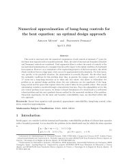
Fig. 1.1: Solutions of the Volterra-Lotka equations (1.1)
is Euler's method
y n+1 = y n + hf(y n ): (1.4)
It is also called explicit Euler method, because the approximation y n+1 can be computed
in an explicit straight-forward way from y n and from the step size h. Here, y n is an
approximation to y(t n ) where y(t) isthe exact solution of (1.3), and t n = t 0 + nh.
The implicit Euler method
y n+1 = y n + hf(y n+1 ) (1.5)
which has its name from its similarity to (1.4), is known from its excellent stability
properties. In contrast to (1.4), the approximation y n+1 is dened implicitly by (1.5), and
the implementation needs the resolution of nonlinear systems.
Taking the mean of y n and y n+1 in the argument of f, we get the implicit midpoint
rule
yn + y n+1
y n+1 = y n + hf
: (1.6)
2
It is a symmetric method, which means that the formula remains the same if we exchange
y n $ y n+1 and h $;h.
For partitioned systems
such as the problem (1.1), we also consider the method
u 0 = a(u v) v 0 = b(u v) (1.7)
u n+1 = u n + ha(u n+1 v n ) v n+1 = v n + hb(u n+1 v n ) (1.8)
which treats the u-variable by the implicit and the v-variable by the explicit Euler method.
It is called symplectic Euler method (in Sect. IV it will be shown that it represents a
symplectic transformation).
Numerical Experiment The result of our rst numerical experiment is shown in
Fig. 1.1. We have applied dierent numerical methods to (1.1), all with constant step
size h = 0:12. As initial values (the enlarged symbols in the pictures) we have chosen
(u 0 v 0 ) = (2 2) for the explicit Euler method, (u 0 v 0 ) = (4 8) for the implicit Euler
method, and (u 0 v 0 ) = (4 2) respectively (6 2) for the symplectic Euler method. The
gure shows the numerical approximations of the rst 125 steps. We observe that the

I Examples and Numerical Experiments 3
explicit and implicit Euler methods behave qualitatively wrong. The numerical solution
either spirals outwards or it spirals inwards. The symplectic Euler method, however, gives
anumerical solution that lies on a closed curve as does the exact solution. It is important
to remark that the curves of the numerical and exact solution do not coincide, but they
will be closer for smaller h. The implicit midpoint rule also shows the correct qualitative
behaviour (we did not include it in the gure).
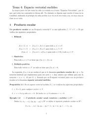
Pendulum Our next problem is the mathematical pendulum with
a massless rod of length ` = 1 and mass m = 1. Its movement is
described by the equation 00 +sin =0. With the coordinates q =
and p = 0 this becomes the two-dimensional system
q 0 = p p 0 = ; sin q: (1.9)
As in the example above we can nd a rst integral, so that all solutions satisfy
`
m
H(p q) = 1 2 p2 ; cos q = Const: (1.10)
Since the vector eld (1.9) is 2-perdiodic in q, it is natural to consider q as a variable
on the circle S 1 . Hence, the phase space of elements (p q) becomes the cylinder IR S 1 .
In Fig. 1.2 level curves of H(p q) are drawn. They correspond to solution curves of the
problem (1.9).
explicit Euler symplectic Euler implicit midpoint
Fig. 1.2: Solutions of the pendulum problem (1.9)
Again we apply our numerical methods: the explicit Euler method with step size
h =0:2 and initial value (p 0 q 0 )=(0 0:5) the symplectic Euler method and the implicit
midpoint rule with h =0:3 and three dierent initial values q 0 = 0 and p 0 2f0:7 1:4 2:1g.
Similar to the computations for the Volterra-Lotka equations we observe that only the
symplectic Euler method and the implicit midpoint rule exhibit the correct qualitative
behaviour. The numerical solution of the midpoint rule is closer to the exact solution,
because it is a method of order 2, whereas the other methods are only of order 1.
Conclusion We have considered two-dimensional problems with the property that all
solutions are periodic. In general, a discretization of the dierential equation destroys
this property. Surprisingly, there exist methods for which the numerical ow shows the
same qualitative behaviour as the exact ow of the problem.

4 I Examples and Numerical Experiments
I.2 Kepler's Problem and the Outer Solar System
The evolution of the entire planetary system has been numerically
integrated for a time span of nearly 100 million years. This calculation
conrms that the evolution of the solar system as a whole is chaotic,
::: (G.J. Sussman and J. Wisdom 1992)
The Kepler problem (also called the two-body problem) describes the motion of two bodies
which attract each other. If we choose one of the bodies as the center of our coordinate
system, the motion will stay in a plane (Exercise 2). Denoting the position of the second
body by q = (q 1 q 2 ) T , Newton's law yields a second order dierential equation which,
with a suitable normalization, is given by
q 1
q 1 = ;
(q 2 1 + q2) q 2 3=2 2 = ;
: (2.1)
(q 2 1 + q2) 2 3=2
One can check that this is equivalent to a Hamiltonian system
q 2
_q = H p (p q) _p = ;H q (p q) (2.2)
(H p and H q are the vectors of partial derivatives) with total energy
H(p 1 p 2 q 1 q 2 )= 1 1
2 (p2 1
+ p 2 2) ; q : (2.3)
q 2 1 + q 2 2
Exact Integration Kepler's problem can be solved analytically, i.e., it can be reduced
to the computation of integrals. This is possible, because the system has not only the
total energy H(p q) asinvariant, but also the angular momentum
L(p 1 p 2 q 1 q 2 )=q 1 p 2 ; q 2 p 1 : (2.4)
This can be checked by dierentiation. Hence, every solution of (2.1) satises the two
relations
1
1
2 (_q2 1
+ _q 2) 2 ; q = H 0 q 1 _q 2 ; q 2 _q 1 = L 0
q 2 1 + q 2 2
where the constants H 0 and L 0 are determined by the initial values. Using polar coordinates
q 1 = r cos ', q 2 = r sin ', this system becomes
1
2 (_r2 + r 2 _' 2 ) ; 1 r = H 0 r 2 _' = L 0 : (2.5)
For its solution we consider r as a function of ' (assuming that L 0 6= 0 so that ' is a
monotonic function). Hence, we have _r = dr _' and the elimination of _' in (2.5) yields
d'
1
dr 2
+ r
2 L
2
0
2 d' r ; 1 4 r = H 0:
With the abbreviations
d = L 2 0 e2 =1+2H 0 L 2 0
(2.6)

I Examples and Numerical Experiments 5
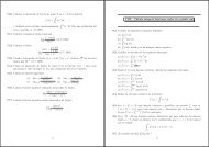
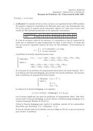
400 000 steps
1
h = 0.0005
−2 −1 1
−2 −1 1
exact solution
−1
explicit Euler
−1
1
implicit midpoint
4 000 steps
h = 0.05
−2 −1 1
−2 −1 1
symplectic Euler
4 000 steps
h = 0.05
−1
Fig. 2.1: Exact and numerical solutions of Kepler's problem
and the substitution u(') =1=r(') we get
du 2 e 2
=
d'
d 2 ; u ; 1 d
This dierential equation can be solved by separation of variables and yields
r(') =
2:
d
1+e cos(' ; ' ) (2.7)
where ' is determined by the initial values r 0 and ' 0 . In the original coordinates this
relation becomes q
q 2 1 + q 2 2 + e(q 1 cos ' + q 2 sin ' )=d:
Eliminating the square root, this gives a quadratic relation for (q 1 q 2 ) which represents
an ellipse with eccentricity e for H 0 < 0 (see Fig. 2.1), a parabola for H 0 = 0, and a
hyperbola for H 0 > 0. With the relation (2.7), the second equation of (2.5) gives
d 2
(1 + e cos(' ; ' )) 2 d' = L 0 dt (2.8)
which, after integration, gives an implicit equation for '(t).
Numerical Integration We consider the problem (2.1) and we choose
s
1+e
q 1 (0) = 1 ; e q 2 (0) = 0 _q 1 (0) = 0 _q 2 (0) =
1 ; e (2.9)

6 I Examples and Numerical Experiments
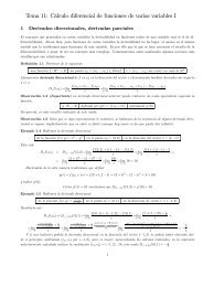
conservation of energy
.02
explicit Euler, h = 0.0001
.01
symplectic Euler, h = 0.001
50 100
.4
.2
global error of the solution
explicit Euler, h = 0.0001
symplectic Euler, h = 0.001
50 100
Fig. 2.2: Energy conservation and global error for Kepler's problem
with 0 e

I Examples and Numerical Experiments 7
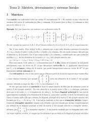
Table 2.2: Data for the outer solar system
planet mass initial position initial velocity
;3:5023653 0:00565429
Jupiter m 1 =0:000954786104043 ;3:8169847 ;0:00412490
;1:5507963 ;0:00190589
9:0755314 0:00168318
Saturn m 2 =0:000285583733151 ;3:0458353 0:00483525
;1:6483708 0:00192462
8:3101420 0:00354178
Uranus m 3 =0:0000437273164546 ;16:2901086 0:00137102
;7:2521278 0:00055029
11:4707666 0:00288930
Neptune m 4 =0:0000517759138449 ;25:7294829 0:00114527
;10:8169456 0:00039677
;15:5387357 0:00276725
Pluto m 5 =1=(1:3 10 8 ) ;25:2225594 ;0:00170702
;3:1902382 ;0:00136504
Outer Solar System We next apply our methods to the system which describes the
motion of the ve outer planets relative to the sun. This system has been studied extensively
by astronomers, who integrated it for a time span of nearly 100 million years and
concluded the chaotic evolution of the solar system [SW92]. The problem is a Hamiltonian
system (2.2) with
H(p q) = 1 2
5X
i=0
m ;1
i
p T i p i ; G
5X Xi;1
i=1 j=0
m i m j
kq i ; q j k : (2.10)
Here p and q are the supervectors composed by the vectors p i q i 2 IR 3 (momenta and
positions), respectively. The chosen units are: masses relative to the sun, so that the sun
has mass 1. We have taken
m 0 =1:00000597682
in order to take account of the inner planets. Distances are in astronomical units (1 [A.U.] =
149 597 870 [km]), times in earth days, and the gravitational constant is
G =2:95912208286 10 ;4 :
The initial values for the sun are taken as q 0 (0) = (0 0 0) T and _q 0 (0) = (0 0 0) T . All
other data (masses of the planets and the initial positions and initial velocities) are given
in Table 2.2. The initial data are taken from \Ahnerts Kalender fur Sternfreunde 1994",
Johann Ambrosius Barth Verlag 1993, and they correspond to September 5, 1994 at 0h00. 1
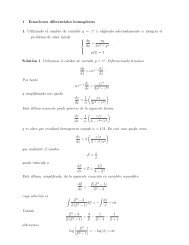
To this system we applied our four methods, all with step size h =10(days) and over
a time period of 200 000 days. The numerical solution (see Fig. 2.3) behaves similarly to
1 We thank Alexander Ostermann, who provided us with all these data.

8 I Examples and Numerical Experiments
explicit Euler, h = 10
implicit Euler, h = 10
P
J
S
P
J
S
U
N
U
N
symplectic Euler, h = 10
implicit midpoint, h = 10
P
J
S
P
J
S
U
N
U
N
Fig. 2.3: Solutions of the outer solar system
that for the Kepler problem. With the explicit Euler method the planets increase their
energy, they spiral outwards, Jupiter approaches Saturn which leaves the plane of the
two-body motion. With the implicit Euler method the planets (rst Jupiter and then
Saturn) fall into the sun and are thrown far away. Both the symplectic Euler method and
the implicit midpoint rule show the correct behaviour. An integration over a much longer
time of say several million of years does not deteriorate this behaviour. Let us remark that
Sussman & Wisdom [SW92] have integrated the outer solar system with special methods
which will be discussed in Chap. IV.
I.3 Molecular Dynamics
We do not need exact classical trajectories to do this, but must lay
great emphasis on energy conservation as being of primary importance
for this reason. (M.P. Allen and D.J. Tildesley 1987)
Molecular dynamics requires the solution of Hamiltonian systems (2.2), where the total
energy is given by
H(p q) = 1 2
NX
i=1
m ;1
i
p T i p i +
NX Xi;1
V ij kqi ; q j k (3.1)
i=2 j=1
and V ij (r) are given potential functions. Here, q i and p i denote the positions and momenta
of atoms and m i is the atomic mass of the ith atom. We remark that the outer solar system
(2.10) is such an N-body system with V ij (r) = ;Gm i m j =r. In molecular dynamics the
Lennard-Jones potential
V ij (r) =4" ij
ij
r
12
;
ij
r
6
(3.2)

I Examples and Numerical Experiments 9
is very popular (" ij and ij are suitable constants
depending on the atoms). This potential has an
absolute minimum at distance r = p .2 Lennard - Jones
6
ij 2. The
.0
force due to this potential strongly repulses the
atoms when they are closer than this value, and
they attract each other when they are farther.
−.2
3 4 5 6 7 8
Stormer-Verlet Scheme The Hamiltonian of (3.1) is of the form H(p q) =T (p)+V (q),
where T (p) is a quadratic function. Hence, the Hamiltonian system is of the form
_q = M ;1 p
_p = ;V 0 (q)
where M = diag(m 1 I:::m N I) and I is the 3-dimensional identity matrix. This system
is equivalent tothe special second order dierential equation
q = f(q) (3.3)
where the right-hand side f(q) = M ;1 V 0 (q) does not depend on _q. The most natural
discretization of (3.3) is 2 q n+1 ; 2q n + q n;1 = h 2 f(q n ): (3.4)
This formula is either called Stormer's method (C. Stormer in 1907 used higher order
variants for the numerical computation concerning the aurora borealis) or Verlet method.
L. Verlet [Ver67] proposed this method for computations in molecular dynamics. An
approximation to the derivative v = _q is simply obtained by
v n = q n+1 ; q n;1
: (3.5)
2h
For the second order problem (3.3) one usually has given initial values q(0) = q 0 and
_q(0) = v 0 . However, one also needs q 1 in order to be able to start the integration with the
3-term recursion (3.4). Putting n = 0 in (3.4) and (3.5), an elimination of q ;1 gives
q 1 = q 0 + hv 0 + h2
2 f(q 0)
for the missing starting value.
The Stormer-Verlet method admits an interesting one-step formulation which is useful
for numerical computations. Introducing the velocity approximation at the midpoint
v n+1=2 := v n + h f(q 2 n), an elimination of q n;1 (as above) yields
v n+1=2 = v n + h 2 f(q n)
q n+1 = q n + hv n+1=2 (3.6)
v n+1 = v n+1=2 + h 2 f(q n+1)
2 Attention. In (3.4) and in the subsequent formulas qn denotes an approximation to q(nh), whereas
qi in (3.1) denotes the ith subvector of q.

10 I Examples and Numerical Experiments
V
which is an explicit one-step method
h
:(q n v n ) 7! (q n+1 v n+1 ) for the rst order system
_q = v _v = f(q). If one is not interested in the values v n of the derivative, the rst and
third equations in (3.6) can be replaced with
v n+1=2 = v n;1=2 + hf(q n ):
Finally, let us mention an interesting connection between the Stormer-Verlet method
and the symplectic Euler method (1.8). If the variable q is discretized by the explicit
ei
Euler and v by the implicit Euler method, we denote it by
h
if q is discretized by
ie
the implicit Euler and v by the explicit Euler method, we denote it by
h
. Introducing
q n+1=2 := q n + h v 2 n+1=2 as an approximation at the midpoint, one recognizes the mapping
ei
(q n v n ) 7! (q n+1=2 v n+1=2 ) as an application of ,and(q h=2 n+1=2v n+1=2 ) 7! (q n+1 v n+1 )as
ie
an application of
h=2
. Hence, the Stormer-Verlet method satises
V
h
=
ie
h=2
Numerical Experiment with a Frozen Argon Crystal
As in [BS93] we consider the interaction of seven argon atoms
in a plane, where six of them are arranged symmetrically
around a center atom. As mathematical model we take the
Hamiltonian (3.1) with N =7,m i = m =66:34 10 ;27 [kg],
" ij = " =119:8 k B [J] ij = =0:341 [nm]
ei
: (3.7)
h=2
where k B =1:38065810 ;23 [J=K] is Boltzmann's constant (see [AT87, page 21]). As units
for our calculations we take masses in [kg], distances in nanometers (1 [nm] =10 ;9 [m]),
and times in nanoseconds (1 [nsec] = 10 ;9 [sec]). Initial positions (in [nm]) and initial
velocities (in [nm=nsec]) are given in Table 3.1. They are chosen such that neighbouring
atoms have a distance that is close to the one with lowest potential energy, and such that
the total momentum is zero and therefore the centre of gravity does not move. The energy
at the initial position is H(p 0 q 0 ) ;1260:2 k B [J].
For computations in molecular dynamics one is usually not interested in the trajectories
of the atoms, but one aims at macroscopic quantities such as temperature, pressure,
internal energy, etc. We are interested in the total energy, given by the Hamiltonian, and
in the temperature which can be calculated from the formula [AT87, page 46]
T = 1 X
N
m i k _q i k 2 : (3.8)
2Nk B i=1
We apply the explicit and symplectic Euler methods and also the Verlet method to this
problem. Observe that for a Hamiltonian such as (3.1) all three methods are explicit, and
7
6
2
1
5
3
4
Table 3.1: Initial values for the simulation of a frozen Argon crystal
atom 1 2 3 4 5 6 7
position
0:00 0:02 0:34 0:36 ;0:02 ;0:35 ;0:31
0:00 0:39 0:17 ;0:21 ;0:40 ;0:16 0:21
velocity
;30 50 ;70 90 80 ;40 ;80
;20 ;90 ;60 40 90 100 ;60

I Examples and Numerical Experiments 11
60 explicit Euler, h = 0.5 [ fsec]
Verlet, h = 40 [ fsec]
30
0
−30
−60
60
30
0
−30
−60
symplectic Euler, h = 10 [ fsec]
total energy
explicit Euler, h = 10 [ fsec]
temperature
total energy
Verlet, h = 80 [ fsec]

II Numerical Integrators 21
Order Conditions for Runge-Kutta Methods Comparing the B-series of the exact
and numerical solutions we see that a Runge-Kutta method has order p, i.e.,y(x 0 + h) ;
y 1 = O(h p+1 ) for all smooth problems (2.1), if and only if
sX
b i i (t) = 1 for (t) p: (2.7)
(t)
i=1
The `only if' part follows from the independency of the elementary dierentials (Exercise
6). This order condition can be immediately read from a tree as follows: attach to
every vertex a summation letter (`i' to the root), then the left-hand expression of (2.7)
is a sum over all summation indices with the summand being a product of b i , and a jk if
the vertex `j' is directly connected with `k' by an upwards leaving branch. For the tree
to the right we thus get
X
ijklmnpqr
or, by using P j a ij = c i ,
b i a ij a jm a in a ik a kl a lq a lr a kp =
X
ijkl
1
9 2 5 3
b i c i a ij c j a ik c k a kl c 2 l
= 1
270 : i
The order conditions up to order 4 can be read from Table 2.1, where i (t) and (t) are
tabulated.
j
m
q
l
n
r
k
p
II.3
Adjoint and Symmetric Methods
For an autonomous dierential equation
y 0 = f(y) y(t 0 )=y 0 (3.1)
the solution y(t t 0 y 0 ) satises y(t t 0 y 0 )=y(t;t 0 0y 0 ). Therefore, it holds for the ow
of the dierential equation, dened by ' t (y 0 )=y(t 0y 0 ), that
' t ' s = ' t+s
and in particular ' 0 = id and ' t ' ;t = id (id is the identity map).
A numerical one-step method is a mapping h : y 0 7! y 1 , which approximates ' h . It
satises 0 = id, it is usually also dened for negative h, and by the inverse function
theorem it is invertible for suciently small h. In the spirit of `geometric integration' it
is natural to study methods which share the property ' t ' ;t = id of the exact ow.
Denition 3.1 A numerical one-step method h is called symmetric, 2 if it satises
h ;h = id or equivalently h = ;1
;h :
The numerical method h := ;1
;h
is called the adjoint method.
2
The study of symmetric methods has its origin in the development of extrapolation methods [Gra64,
Ste73], because the global error admits an asymptotic expansion in even powers of h.

22 II Numerical Integrators
The adjoint operator satises the usual properties such as( h) = h and ( h h) =
h h for any two one-step methods h and h.
For the computation of the adjoint method we observe that y 1 = h(y 0 ) is implicitly
dened by ;h (y 1 ) = y 0 , i.e., y 1 is the value which yields y 0 when the method h is
applied with negative step size ;h. For example, the explicit Euler method in the role of
h gives y 1 ; hf(y 1 )=y 0 ,andwe see that the adjoint of the explicit Euler method is the
implicit Euler method. The implicit midpoint rule (I.1.6) is invariant with respect to the
transformation y 0 $ y 1 and h $;h. Therefore, it is a symmetric method.
Theorem 3.2 Let ' t be the exact ow of (3.1) and let h be a one-step method of order
p satisfying
h (y 0 )=' h (y 0 )+C(y 0 )h p+1 + O(h p+2 ): (3.2)
Then, the adjoint method h
has the same order p and it holds that
h(y 0 )=' h (y 0 )+(;1) p C(y 0 )h p+1 + O(h p+2 ): (3.3)
Moreover, if h is symmetric, its (maximal) order is even.
Proof.
We replace h and y 0 in Eq. (3.2) by ;h and ' h (y 0 ), respectively. This gives
;h
' h (y 0 ) = y 0 + C
' h (y 0 ) (;h) p+1 + O(h p+2 ): (3.4)
Since ' h (y 0 ) = y 0 + O(h) and 0 ;h(y 0 ) = I + O(h), it follows from the inverse function
theorem that ( ;1
;h) 0 (y 0 )=I + O(h). Applying the function ;1
;h
to (3.4) yields
' h (y 0 ) = ;1
;h
y
0 + C(' h (y 0 ))(;h) p+1 + O(h p+2 )
= h(y 0 )+C(y 0 )(;h) p+1 + O(h p+2 )
implying (3.3). The statement for symmetric methods is an immediate consequence of
this result, because h = h implies C(y 0 ) = (;1) p C(y 0 ), and therefore C(y 0 ) can be
dierent from zero only for even p.
Theorem 3.3 ([Ste73, Wa73]) The adjoint method ofan s-stage Runge-Kutta method
(1.2) is again an s-stage Runge-Kutta method. Its coecients are given by
If
the Runge-Kutta method (1.2) is symmetric. 3
a ij
= b s+1;j ; a s+1;is+1;j b i
= b s+1;i : (3.5)
a s+1;is+1;j + a ij = b j for all i j, (3.6)
Proof. Let h denote the Runge-Kutta method (1.2). The numerical solution of the
adjoint method y 1 = h(y 0 ) is given by y 0 = ;h (y 1 ). By exchanging y 0 $ y 1 and
h $;h we thus obtain
sX
sX
k i = f y 0 + h (b j ; a ij )k j
y 1 = y 0 + h b i k i : (3.7)
j=1
Since the values P s
j=1(b j ; a ij )=1; c i appear in reverse order, we replace k i by k s+1;i
in (3.7), and then we substitute all indices i and j by s +1; i and s +1; j, respectively.
This proves (3.5).
The assumption (3.6) implies a ij = a ij and b i = b i ,sothat h = h .
i=1
3
For irreducible Runge-Kutta methods, the condition (3.6) is also necessary for symmetry (after a
suitable permutation of the stages).

II Numerical Integrators 23
For the methods of Table 1.1 one can directly check that the condition (3.6) holds.
Furthermore, all Gauss methods are symmetric (Exercise 10).
II.4
Partitioned Runge-Kutta Methods
Some interesting numerical methods introduced in Chapter I (symplectic Euler and the
Stormer-Verlet method) do not belong to the class of Runge-Kutta methods. They are
important examples of so-called partitioned Runge-Kutta methods. In this section we
consider dierential equations in the partitioned form
p 0 = f(p q) q 0 = g(p q): (4.1)
We have chosen the letters p and q for the dependent variables, because Hamiltonian
systems (I.2.2) are of this form and they are of particular interest in this lecture.
Denition 4.1 Let b i a ij and b i ba ij be the coecients of two Runge-Kutta methods. A
partitioned Runge-Kutta method for the solution of (4.1) is given by
sX
sX
k i = f
p 0 + h
`i = g p 0 + h
p 1 = p 0 + h
sX
i=1
sX
j=1
j=1
a ij k j q 0 + h
a ij k j q 0 + h
sX
j=1
j=1
ba ij`j
ba ij`j
b i k i q 1 = q 0 + h
sX
i=1
b bi`i:
(4.2)
Methods of this type have originally been proposed by Hofer (1976) and Griepentrog
(1978) for problems with sti and nonsti parts (see [HNW93, Sect. II.15]). Their
importance for Hamiltonian systems has been discovered only very recently.
An interesting example is the symplectic Euler method (I.1.8), where the implicit
Euler method b 1 =1a 11 =1is combined with the explicit Euler method b b 1 =1 ba 11 =0.
The Stormer-Verlet method (I.3.6) is of the form (4.2) with coecients given in Table 4.1.
The theory of Runge-Kutta methods can be extended in a straight-forward way to
partitioned methods. Since (4.2) is a one-step method (p 1 q 1 )= h (p 0 q 0 ), the order, the
adjoint method and symmetric methods are dened in the usual way.
Explicit Symmetric Methods An interesting feature of partitioned Runge-Kutta
methods is the possibility ofhaving explicit, symmetric methods for problems of the form
p 0 = f(q) q 0 = g(p) (4.3)
e.g., if the problem is Hamiltonian with separable H(p q) = T (p) +V (q). This is not
possible with classical Runge-Kutta methods (Exercise 9).
Table 4.1: Stormer-Verlet as partitioned Runge-Kutta method
0 0 0
1 1=2 1=2
1=2 1=2
1=2 1=2 0
1=2 1=2 0
1=2 1=2

24 II Numerical Integrators
Exactly as in the proof of Theorem 3.3 one can show that the partitioned method
(4.2) is symmetric, if both Runge-Kutta methods are symmetric, i.e., if the coecients
of both methods satisfy (3.6). The method is explicit for problems (4.3), if a ij = ba ij =0
for i

II Numerical Integrators 25
Table 4.2: Bi-colored trees, elementary dierentials, and coecients
(t) t graph (t) (t) F (t) i (t)
1 p 1 1 f 1
2 [ p ] p 1 2 f p f
2 [ q ] p 1 2 f q g
3 [ p p ] p 1 3 f pp (f f)
3 [ p q ] p 2 3 f pq (f g)
3 [ q q ] p 1 3 f qq (g g)
3 [[ p ] p ] p 1 6 f p f p f
3 [[ q ] p ] p 1 6 f p f q g
3 [[ p ] q ] p 1 6 f q g p f
3 [[ q ] q ] p 1 6 f q g q g
P
P
P
P
P
P
P
P
j a ij
j
ba ij
jk a ij a ik
jk a ij ba ik
jk
ba ij ba ik
jk a ij a jk
jk a ij ba jk
jk
ba ij a jk
P
jk
ba ij ba jk
Denition 4.2 (P-Series) For a mapping a : TP [f p q g!IR a series of the form
0
Pp (a (p q))
P a (p q) =
= @ a( p)p + P 1
h (t)
t2TP p
(t) a(t) F (t)(p q)
(t)!
P q (a (p q)) a( q )q + P A
h (t)
t2TP (t) a(t) F (t)(p q) q (t)!
is called a P-series.
The following results are obtained in exactly the same manner as the corresponding
results for non-partitioned Runge-Kutta methods (Sect. II.2). We therefore omit their
proofs.
Lemma 4.3 Let a : TP [f p q g!IR satisfy a( p )=a( q )=1. Then, it holds
!
f(P (a (p q)))
h
= P a 0 (p q)
g(P (a (p q)))
where a 0 ( p )=a 0 ( q )=0, a 0 ( p )=a 0 ( q )=1, and
if either t =[t 1 :::t m ] p or t =[t 1 :::t m ] q .
a 0 (t) =(t) a(t 1 ) ::: a(t m ) (4.6)
Theorem 4.4 (P-Series of Exact Solution) The exact solution of (4.1) is a P-series
(p(x 0 + h)q(x 0 + h)) = P (e (p 0 q 0 )), where e( p )=e( q )=1and
e(t) =1 for all t 2 TP: (4.7)

26 II Numerical Integrators
Theorem 4.5 (P-Series of Numerical Solution) The numerical solution of a partitioned
Runge-Kutta method (4.2) is a P-series (p 1 q 1 ) = P (a (p 0 q 0 )), where a( p ) =
a( q )=1and
a(t) =
( (t)
P s
i=1 b i i (t) for t 2 TP p
(t) P s
i=1
b bi i (t) for t 2 TP q :
(4.8)
The integer coecient (t) is the same as in (2.5). It does not depend on the color of the
vertices. The expression i (t) is dened by i ( p )= i ( q )=1and by
i (t) = i(t 1 ) ::: i(t m ) with i(t k )=
for t =[t 1 :::t m ] p or t =[t 1 :::t m ] q .
( P s
j k =1 a ij k
jk (t k ) if t k 2 TP p
Ps
j k =1 ba ij k
jk (t k ) if t k 2 TP q
(4.9)
Order Conditions Comparing the P-series of the exact and numerical solutions we see
that a partitioned Runge-Kutta method (4.2) has order r, i.e.,p(x 0 + h) ; p 1 = O(h r+1 ),
q(x 0 + h) ; q 1 = O(h r+1 ), if and only if
sX
sX
i=1
i=1
b i i (t) = 1
(t)
b bi i (t) = 1
(t)
for t 2 TP p with (t) r
for t 2 TP q with (t) r.
(4.10)
This means that not only every individual Runge-Kutta method has to be of order r, but
also so-called coupling conditions between the coecients of both methods have to hold.
As in Sect. II.2 the order conditions can be directly read from the trees: we attach
to every vertex a summation letter (`i' to the root). Then the left-hand expression of
(4.10) is a sum over all summation indices with the summand being a product of b i or b b i
(depending on whether the root is black or white) and of a jk (if `k' isblack) or ba jk (if `k'
is white), if the vertex `k' is directly above `j'. For the tree to the right we thus obtain
X
ijklmnpqr
b i ba ij ba jm ba in a ik ba kl a lq a lr a kp =
or, by using P j a ij = c i and P j
ba ij = bc i ,
X
ijkl
1
9 2 5 3
b i bc i ba ij bc j a ik c k ba kl c 2 l = 1
270 : i
The order conditions up to order 3 can be read from Table 4.2, where i (t) and (t) are
tabulated.
Example 4.6 (Lobatto IIIA - IIIB Pair) We let c 1 :::c s be the zeros of
d s;2
x s;1 (x ; 1)
s;1
dx s;2
and we consider the interpolatory quadrature formula (b i c i ) s i=1
based on these nodes. The
special cases s = 2 and s = 3 are the trapezoidal rule and Simpson's rule. We then dene
the Runge-Kutta coecients a ij (Lobatto IIIA) and ba ij (Lobatto IIIB) by the following
conditions (see Sect. II.2 for the denition of B(p) andC(q)):
j
m
q
l
n
r
k
p

II Numerical Integrators 27
Lobatto IIIA B(2s ; 2), C(s) \collocation"
Lobatto IIIB
B(2s ; 2), C(s ; 2) and ba i1 = b 1 ba is =0fori =1:::s.
For s =2we get the Stormer-Verlet method of Table 4.1. The coecients of the methods
for s =3aregiven in Table 4.3. One can prove that this partitioned Runge-Kutta method
is of order p =2s ; 2. Instead of giving the general proof (see e.g., [HW96, page 563]) we
check the order for the case s =3. Due to the simplifying assumptions C(s) for Lobatto
IIIA and C(s ; 2) for Lobatto IIIB the order conditions for all bi-colored trees up to
order 3 are immediately veried (using the expressions of Table 4.2). Order 4 is then a
consequence of Theorem 3.2 and the fact that both Runge-Kutta methods are symmetric.
II.5
Nystrom Methods
as important special case of partitioned Runge-Kutta methods, M.P. Calvo
II.6
Methods Obtained by Composition
An interesting means for the construction of higher order integration methods is by composition
of simple methods. We have already seen in Chapter I that the Stormer-Verlet
method can be considered as the composition of two symplectic Euler methods. The
results of this section are valid for general one-step methods (partitioned as well as nonpartitioned
ones).
Theorem 6.1 ([Yo90]) Let h (y) be a symmetric one-step method of order p =2k. If
then the composed method
is symmetric and has order p =2k +2.
2b 1 + b 0 =1 2b 2k+1
1
+ b 2k+1
0
=0 (6.1)
h = b1 h b0 h b1 h
Proof. The basic method satises h (y 0 )=' h (y 0 )+C(y 0 )h 2k+1 +O(h 2k+2 ), where ' t (y 0 )
denotes the exact ow of the problem. Consequently, it holds
b1 h b2 h b3 h(y 0 )=' (b1 +b 2 +b 3 )h(y 0 )+(b 2k+1
1
+ b 2k+1
2
+ b 2k+1
3
)C(y 0 )h 2k+1 + O(h 2k+2 ):
The assumption (6.1) thus implies order at least 2k +1 for the composed method h.
Due to b 3 = b 1 and the symmetry of h , the method h is also symmetric, implying that
the order of h is at least 2k +2(Theorem 3.2).
Table 4.3: Coecients of the 3-stage Lobatto IIIA -IIIBpair
0 0 0 0
1=2 5=24 1=3 ;1=24
1 1=6 2=3 1=6
1=6 2=3 1=6
0 1=6 ;1=6 0
1=2 1=6 1=3 0
1 1=6 5=6 0
1=6 2=3 1=6

28 II Numerical Integrators
The above theorem allows us to construct symmetric one-step methods of arbitrarily
high order. We take a symmetric method (2)
h
of order 2, e.g., the implicit midpoint rule
(I.1.6) or the Stormer-Verlet method (I.3.6) or something else. With the choice
b 1 =(2; 2 1=3 ) ;1
b 0 =1; 2b 1
the method (4)
h
:= (2)
b 1 h (2) b 0 h (2) b 1 h
is symmetric and of order 4 (see Theorem 6.1).
Observethatb 1 1:3512072 and b 0 ;1:7024144. This means that the method takes two
positive stepsizes b 1 h and one negative step size b 0 h. We can now repeat this procedure.
With c 1 = (2 ; 2 1=5 ) ;1 and c 0 = 1 ; 2c 1 , the method (6)
h
:= (4)
c 1 h
(4)
c 0 h
(4)
c 1 h
is
symmetric and of order 6. For every step it requires 9 applications of the basic method
(2)
h
. Continuing this procedure, we can construct symmetric methods of order p = 2k
which require 3 k;1 applications of (2)
h
.
If we take as basic method the Stormer-Verlet method and if the dierential equation is
of the special type (4.3), then we obtain by this construction explicit symmetric methods
of arbitrarily high order. The implementation of these methods is extremely simple. One
only has to write a subroutine for the basic method of low order and one calls it several
times with dierent step sizes.
Optimal Composition Methods The methods constructed above are of the form
h = bmh ::: b1 h b0 h b1 h ::: bmh (6.2)
with m = 1 for the 4th order method, m = 4 for the 6th order method, and m = 13
for the 8th order method. It is natural to ask for optimal methods in the sense that a
minimal number of bi h (i.e., minimal m) is required for a given order.
There are several ways of nding the order conditions. One approach is that adopted
in the proof of Theorem 6.1. In this way one sees that for a second order method h the
composition h of (6.2) is of order at least 4if
b 0 +2(b 1 + :::+ b m ) = 1
b 3 0
+2(b 3 1
+ :::+ b 3 m) = 0:
(6.3)
An extension of this approach to higher order is rather tedious. It is surprising that for
order 6onlytwo additional order conditions
b 5 0
+2(b 5 1
+ :::+ b 5 m) = 0
P m
j=1(B j;1 b 4 j + B 2 j;1 b3 j ; C j;1 b 2 j ; B j;1 C j;1 b j ) = 0
(6.4)
where B j = b 0 +2(b 1 +:::+b j )andC j = b 3 0
+2(b 3 1
+:::+b 3 j), have to be satised (compare
with the large number of conditions for Runge-Kutta methods). We do not give details of
the derivation of (6.4), because later in Chapter IV we shall see a very elegant approach
to these order conditions with the help of backward error analysis and with the use of the
Campbell-Baker-Hausdor formula. It is interesting to note that the order conditions for
(6.2) do not depend on the basic method h .

II Numerical Integrators 29
Example 6.2 For a method (6.2) of order 6 the coecients b i have to satisfy the four
conditions (6.3) and (6.4). Yoshida [Yo90] solves these equations numerically with m =3.
He nds three solutions, one of which is
b 1 = ;1:17767998417887
b 2 = 0:235573213359357
b 3 = 0:784513610477560
and b 0 =1; 2(b 1 + b 2 + b 3 ).
A method of order 8withm =7isalso constructed in [Yo90].
II.7
Linear Multistep Methods
In 1984 a graduate student, who took my ODE class at Stanford,
wanted to work with symmetric multistep methods. I discouraged
him, ::: 4 (G. Dahlquist in a letter to the author, 22. Feb. 1998)
symmetric, with a motivation, partitioned, underlying one-step method, Kirchgraber
II.8
Exercises
1. Compute all collocation methods with s = 2 in dependence of c 1 and c 2 . Which of them
are of order 3, which of order 4?
2. Prove that the collocation solution plotted in the right picture of Fig. 1.1 is composed of
arcs of parabolas.
3. Find all trees of orders 5 and 6.
4. (A. Cayley [Ca1857]) Denote the number of trees of order q by a q . Prove that
a 1 + a 2 x + a 3 x 2 + a 4 x 3 + ::: =(1; x) ;a 1
(1 ; x 2 ) ;a 2
(1 ; x 3 ) ;a3 ::: :
q 1 2 3 4 5 6 7 8 9 10
a q 1 1 2 4 9 20 48 115 286 719
5. Prove that the coecient (t) of Denition 2.2 is equal
to the number of possible monotonic labellings of the
vertices of t, starting with the label 1 for the root.
For example, the tree [[]] has three dierent monotonic
labellings.
3 2
1
4
2 3
1
4
2 4
6. Show that for every t 2 T there is a system (2.1) such that the rst component ofF (t)(0)
equals 1, and the rst component ofF (u)(0) is zero for all trees u 6= t.
Hint. Consider a monotonic labelling of t, and dene y 0 i as the product over all y j, where
j runs through all labels of vertices that lie directly above the vertex `i'. For the rst
labelling of the tree of Exercise 5 this would be y 0 1
= y 2 y 3 , y 0 2
=1,y 0 3
= y 4 ,andy 0 4
=1.
7. Compute the adjoint of the symplectic Euler method (I.1.8).
4 ::: because Dahlquist had proved the result that stable symmetric multistep methods with positive
growth parameters have an order at most 2. We shall see later that certain partitioned multistep methods
can have an excellent long-time behaviour.
1
3

30 II Numerical Integrators
8. Prove that the Stormer-Verlet method (I.3.6) is symmetric.
Hint. If h is the adjoint method of h , then the compositions h=2 h=2 and h=2 h=2
are symmetric one-step methods.
9. Explicit Runge-Kutta methods cannot be symmetric.
Hint. If a one-step method applied to y 0 = y yields y 1 = R(h)y 0 then, a necessary
condition for the symmetry of the method is R(z)R(;z) = 1 for all complex z.
10. A collocation method is symmetric if and only if (after a suitable permutation of the c i )
c i + c s+1;i = 1 holds for all i, i.e., the collocation points are symmetrically distributed on
the interval [0 1].
11. Consider a one-step method h of order 2. Is it possible to construct a composition
method h = b1 h ::: bmh of order at least 3 under the restriction that all b i are
positive?
12. The number of order conditions for partitioned Runge-Kutta methods (4.2) is 2a r for
order r, where a r is given by (see [HNW93, page 311])
r 1 2 3 4 5 6 7 8 9 10
a r 1 2 7 26 107 458 2058 9498 44987 216598
Find a formula similar to that of Exercise 4.
13. Let fb i a ij g and fe bi ea ij g be the coecients of two Runge-Kutta methods h and e h ,
respectively. Prove that the composition h e (1;)h is again a Runge-Kutta method.
What are its coecients?
14. If h stands for the implicit midpoint rule, what are the Runge-Kutta coecients of the
composition method (6.2)? The general theory of Sect. II.2 gives three order conditions for
order 4 (those for the trees of order 2 and 4 are automatically satised by the symmetry
of the method). Are they compatible with the two conditions (6.3)?

Chapter III
Exact Conservation of Invariants
This chapter is devoted to the conservation of invariants (rst integrals) by numerical
methods. Our investigation will followtwo directions. We rst study which of the methods
introduced in Chapter II conserve rst integrals automatically. We shall see that most
of them conserve linear invariants, a few of them quadratic invariants, and none of them
conserves cubic or general nonlinear invariants. We then construct new classes of methods,
which are adapted to known invariants and which force the numerical solution to satisfy
them. In particular, we study projection methods and so-called Lie group methods which
are based on the Magnus expansion of the solution of non-autonomous linear systems.
III.1
Examples of First Integrals
Consider a dierential equation
where y is avector or eventually a matrix.
y 0 = f(y) y(t 0 )=y 0 (1.1)
Denition 1.1 A non-constant function I(y) is called a rst integral of (1.1) if
I 0 (y)f(y)=0 for all y: (1.2)
This implies that every solution y(t) of(1.1) satises I(y(t)) = I(y 0 )=Const.
In Chapter I we have seenmany examples of dierential equations with rst integrals.
E.g., The Volterra-Lotka problem (I.1.1) has I(u v) =lnu;u+2lnv ; v as rst integral.
The pendulum equation (I.1.9) has H(p q) =p 2 =2;cos q, and the Kepler problem (I.2.1)
has even two rst integrals, namely H and L of (I.2.3) and (I.2.4), respectively.
Example 1.2 (Conservation of the Total Energy) Every Hamiltonian system 1
p 0 = ;H T q (p q) q 0 = H T p (p q)
has the Hamiltonian function H(p q)asrstintegral. This follows at once from H 0 (p q) =
(H p H q ) and H p (;H q ) T + H q H T p =0.
1 In contrast to the notation of the previous chapters we are here consistent with the usual notation
and we write the vector of partial derivatives Hp asarowvector.

32 III Exact Conservation of Invariants
Example 1.3 (Conservation of Mass in Chemical Reactions) Suppose that three
substances A, B, C undergo achemical reaction such as 2
A
B + B
B + C
0:04
;;! B (slow)
3107
;;! C + B (very fast)
10
;;! 4
A + C (fast).
We denote the masses (or concentrations) of the substances A, B, C by y 1 , y 2 , y 3 , respectively.
By the mass action law this leadstotheequations
A: y 0 1
= ; 0:04y 1 +10 4 y 2 y 3 y 1 (0) = 1
B: y 0 2
= 0:04y 1 ; 10 4 y 2 y 3 ; 3 10 7 y 2 2
y 2 (0) = 0
C: y 0 3
= 3 10 7 y 2 2
y 3 (0) = 0:
One can check that the total mass I(y) =y 1 + y 2 + y 3 is arstintegral of the system.
Theorem 1.4 (Conservation of Linear First Integrals [Sh86]) All explicit and implicit
Runge-Kutta methods as well as multistep methods conserve linear rst integrals.
Partitioned Runge-Kutta methods (II.4.2) conserve linear rst integrals only if b i = b b i
for all i, or if the rst integral only depends on p alone or only on q alone.
Proof. Let I(y) =d T y with a constantvector d. The assumption (1.2) implies d T f(y) =0
for all y. In the case of Runge-Kutta methods we thus have d T k i =0,and consequently
d T y 1 = d T y 0 + hd T ( P s
i=1 b ik i ) = d T y 0 . The statement for multistep methods and partitioned
methods is proved similarly.
Next we consider dierential equations of the form
Y 0 = B(Y )Y Y (t 0 )=Y 0 (1.3)
where Y can be a vector, but usually it will be a square matrix. We then have the
following result.
Theorem 1.5 If B(Y ) is skew-symmetric for all Y (i.e., B T = ;B), then the quadratic
function I(Y )=Y T Y is a rst integral. In particular, if the initial value is an orthogonal
matrix (i.e., Y T
0 Y 0 = I), then the solution Y (t) of (1.3) remains orthogonal for all t.
Proof. The derivativeofI(Y )isI 0 (Y )H = Y T H +H T Y . Since B(Y )isaskew-symmetric
matrix, we have I 0 (Y )f(Y ) = I 0 (Y )(B(Y )Y ) = Y T B(Y )Y + Y T B(Y ) T Y = 0 for all Y .
This proves the statement.
Example 1.6 (Rigid Body Simulation) Consider a rigid body whose center of mass
is xed at the origin. Its movement is described by the Euler equations
y 0 1
= a 1 y 2 y 3 a 1 = (I 2 ; I 3 )=(I 2 I 3 )
y 0 2
= a 2 y 3 y 1 a 2 = (I 3 ; I 1 )=(I 3 I 1 ) (1.4)
y 0 3
= a 3 y 1 y 2 a 3 = (I 1 ; I 2 )=(I 1 I 2 )
where the vector y =(y 1 y 2 y 3 ) T
represents the angular momentum in the body frame,
2 This problem is very popular in testing codes for sti dierential equations.

III Exact Conservation of Invariants 33
and I 1 I 2 I 3 are the principal moments of inertia (see [MaR94, Chap. 15] for a detailed
description). This problem can be written as
0
B
@
y 0 1
y 0 2
y 0 3
1
C
A =
0
B
@
0 I ;1
3 y 3 ;I ;1
2 y 2
;I ;1
3 y 3 0 I ;1
1 y 1
I ;1
2 y 2 ;I ;1
1 y 1 0
1 0
C
A
B
@
1
y 1
C
y 2 A (1.5)
y 3
which is of the form (1.3) with a skew-symmetric matrix B(Y ). By Theorem 1.5, y 2 1
+
y 2 2
+ y 2 3
is a rst integral. It is interesting to note that the system (1.4) is actually a
Hamiltonian system on the sphere fy 2 1
+ y 2 2
+ y 2 3
=1g with Hamiltonian
H(y 1 y 2 y 3 )= 1 2
y
2
1
I 1
+ y2 2
I 2
+ y2 3
I 3
:
This is a second quadratic invariant ofthe system (1.4).
implicit midpoint
explicit Euler
Fig. 1.1: Solutions of the Euler equations (1.4) for the rigid body
Inspired by the cover page of [MaR94], we present in Fig. 1.1 the sphere with some of
the solutions of (1.4) corresponding to I 1 = 2, I 2 = 1 and I 3 = 2=3. In the left picture
we have included the numerical solution (30 steps) obtained by the implicit midpoint rule
with step size h = 0:3 and initial value y 0 = (cos(1:1) 0 sin(1:1)) T . It stays exactly on
a solution curve. This follows from the fact that the implicit midpoint rule preserves
quadratic invariants exactly (Sect. III.3).
For the explicit Euler method (right picture, 320 steps with h = 0:05 and the same
initial value as above) we see that the numerical solution shows the wrong qualitative
behaviour (it should lie on a closed curve). The numerical solution even drifts away from
the manifold.

34 III Exact Conservation of Invariants
III.2
Dierential Equations on Lie Groups
Theorem 1.5 is a particular case of a more general result, which can be conveniently
formulated with the concept of Lie groups and Lie algebras (see [Olv86] and [Var74] for
an introduction to this subject).
Denition 2.1 A Lie group is a group G which is a dierentiable manifold, and for which
the product is a dierentiable mapping G G ! G.
If I is the unit element of G, then the tangent space T I G is called the Lie algebra of
G and it is denoted by g.
We restrict our considerations to matrix Lie groups (Table 2.1). The matrix J, appearing
in the denition of the symplectic group, is the matrix determining the symplectic
structure on R n (see Chapter IV).
Table 2.1: Some matrix Lie groups and their corresponding Lie algebras
Lie group
Lie algebra
GL(n) = fA j det A 6= 0g gl(n) = fB j arbitrary matrixg
general linear group
Lie algebra of n n matrices
SL(n) = fA j det A =1g sl(n) = fB j trace(B) =0g
special linear group
special linear Lie algebra
O(n) = fA j A T A = Ig so(n) = fB j B T + B =0g
orthogonal group
skew-symmetric matrices
SO(n) = fA 2 O(n) j det A =1g so(n) = fB j B T + B =0g
special orthogonal group
skew-symmetric matrices
Sp(n) = fA j A T JA = Jg sp(n) = fB j JB + B T J =0g
symplectic group
Example 2.2 An interesting example of a Lie group is the set
O(n) =fA 2 GL(n) j A T A = Ig
of all orthogonal matrices. It is the kernel of g(A) = A T A ; I, where we consider g
as a mapping from the set of all n n matrices (i.e., IR nn ) to the set of all symmetric
matrices (which can be identied with IR n(n+1)=2 ). The derivative g 0 (A) is surjective
for A 2 O(n), because for any symmetric matrix K the choice H = AK=2 solves the
equation g 0 (A)H = K. Therefore, O(n) denes a dierentiable manifold of dimension
n 2 ; n(n +1)=2 = n(n ; 1)=2. The set O(n) is also a group with unit element I (the
identity). Since the matrix multiplication is a dierentiable mapping, O(n) is a Lie group.
In order to compute its Lie algebra, we use the fact that for manifolds, which are
dened as the kernel of a mapping g, the tangent space is given by T I O(n) =Kerg 0 (I).
Since g 0 (I)H = I T H + H T I = H + H T , it consists of all skew-symmetric matrices.

III Exact Conservation of Invariants 35
Lemma 2.3 (Exponential Map) Consider a Lie group G and its Lie algebra g. The
exponential function
exp(B) = X k0
1
k! Bk
is a map exp : g ! G, i.e., for B 2 g we have exp(B) 2 G.
Proof.
For B 2 g, it follows from the denition of the tangent space g = T I G that there
exists a dierentiable mapping :(;" ") ! G satisfying (0) = I and 0 (0) = B. For a
xed Y 2 G, the function : (;" ") ! G, dened by (t) := (t)Y , satises (0) = Y
and 0 (0) = BY . Consequently, BY 2 T Y G and Y 0 = BY denes a dierential equation
on the manifold G. The solution Y (t) =exp(tB) is therefore in G.
The next lemma motivates the name \Lie algebra" for the tangent space T I G.
Lemma 2.4 (Lie Bracket) Let G be aLiegroup and g its Lie algebra. The Lie bracket
(or commutator)
[A B] =AB ; BA (2.1)
denes an operation gg ! g which is bilinear, skew-symmetric ([A B] =;[B A]), and
satises the Jacobi identity
[A [B C]]+[C [A B]] + [B[C A]] = 0: (2.2)
Proof.
For A B 2 g, we consider the mapping :(;" ") ! G, dened by
(t) =exp( p tA) exp( p tB)exp(; p tA) exp(; p tB):
Using exp( p tA) =I + p tA+ 1 2 tA2 +O(t 3=2 ), an elementary computation yields (t) =I +
t[A B]+O(t 3=2 ). This is a dierentiable mapping satisfying (0) = I and 0 (0) = [A B].
Hence [A B] 2 g by denition of the tangent space. The properties of the Lie bracket
can be veried straight-forwardly.
Theorem 2.5 Let G be a Lie group and g its Lie algebra. If B(Y ) 2 g for all Y 2 G
and if Y 0 2 G, then the solution of (1.3) satises Y (t) 2 G for all t.
If in addition B(Y ) 2 g for all matrices Y , and if G = fY j g(Y )=Constg is one of
the Lie groups of Table 2.1, then g(Y ) is a rst integral of the dierential equation (1.3).
Proof. As in the proof of Lemma 2.3 we see that B(Y )Y 2 T Y G, so that (1.3) is a
dierential equation on the manifold G.
The second statement has already been proved in Theorem 1.5 for G = O(n). Let
us prove it for SL(n). For B 2 g we let (t) as in the proof of Lemma 2.3, and we
put (t) = (t)Y . In general, (t) will not be in G, but it holds g((t)) = det((t)) =
det((t)) det Y = Const det Y . Dierentiation with respect to t gives g 0 (Y )(BY )=0for
all Y , which means that g(Y ) is a rst integral of (1.3).

36 III Exact Conservation of Invariants
III.3
Quadratic Invariants
Quadratic rst integrals appear often in applications. Examples are: the conservation
law of angular momentum (L(p q) in Kepler's problem (I.2.1) and L(p q) = P N
i=1 q i p i
in the Hamiltonian systems (I.2.10) and (I.3.1)), the two invariants in the rigid body
simulation (Example 1.6), and the rst integrals Y T Y ; I and Y T JY ; J of Theorem 2.5.
We therefore consider dierential equations (1.1) and quadratic functions
where C is a symmetric square matrix.
Q(y) =y T Cy (3.1)
Theorem 3.1 The Gauss methods of Example II.1.7 (collocation based on the shifted
Legendre polynomials) conserve quadratic rst integrals.
Proof. Let u(t) be the collocation polynomial (Denition II.1.3). Since d Q(u(t)) =
dt
2u(t) T Cu 0 (t), it follows from u(t 0 )=y 0 and u(t 0 + h) =y 1 that
y T 1 Cy 1
; y T 0 Cy 0
=2
Z t0 +h
t 0
u(t) T Cu 0 (t) dt: (3.2)
The integrand u(t) T Cu 0 (t) is a polynomial of degree 2s ; 1, which is integrated without
error bythes-stage Gaussian quadrature formula. It therefore follows from Cu 0 (t 0 +c i h)=
Cf(u(t 0 + c i h)) = 0 that the integral in (3.2) vanishes.
Since the implicit midpoint rule is the special case s = 1 of the Gauss methods, the
preceding theorem explains its good behaviour for the rigid body simulation in Fig 1.1.
Theorem 3.2 ([Co87]) If the coecients of a Runge-Kutta method satisfy
then it conserves quadratic rst integrals. 3
b i a ij + b j a ji = b i b j for all i j =1:::s (3.3)
Proof. The proof is the same as that for B-stability, given independently by Burrage &
Butcher and Crouzeix in 1979 (see [HW96, Sect. IV.12]).
The relation y 1 = y 0 + P s
h
i=1 b ik i of Denition II.1.1 yields
y T 1 Cy 1
= y T 0 Cy 0
+ h
sX
i=1
b i k T i Cy 0 + h
sX
j=1
b j y T 0 Ck j + h 2
sX
ij=1
b i b j k T i Ck j: (3.4)
We then write k i = f(Y i ) with Y i = P s
y 0 +h
j=1 a ijk j . The main idea is now to compute y 0
from this relation and to insert it into the central expressions of (3.4). This yields (using
the symmetry of C)
sX
sX
y T 1 Cy 1
= y T 0 Cy 0
+2h b i Y T
i Cf(Y i )+h 2 (b i b j ; b i a ij ; b j a ji ) k T i Ck j:
i=1
The condition (3.3) together with the assumption y T Cf(y) =0,which states that y T Cy
is a rst integral of (1.1), imply y T 1 Cy 1
= y T 0 Cy 0.
ij=1
3 For irreducible Runge-Kutta methods the condition (3.3) is also necessary for the conservation of
quadratic rst integrals.

III Exact Conservation of Invariants 37
We next consider partitioned Runge-Kutta methods for systems p 0 = f(p q), q 0 =
g(p q). Usually such methods will not conserve general quadratic invariants (Exercise 6).
We therefore concentrate on quadratic rst integrals of the form
Q(p q) =p T Dq (3.5)
where D is an arbitrary matrix. Observe that the angular momentum in the Hamiltonian
systems (I.2.10) and (I.3.1) is of this form.
Theorem 3.3 If the coecients of a partitioned Runge-Kutta method (II.4.2) satisfy
b i ba ij + b b j a ji = b i
b bj for i j =1:::s (3.6)
b i = b b i for i =1:::s (3.7)
then it conserves quadratic rst integrals of the form (3.5).
If the partitioned dierential equation is of the special form p 0 = f(q), q 0 = g(p), then
the condition (3.6) alone implies that rst integrals of the form (3.5) are conserved.
Proof.
The proof is nearly identical to that of Theorem 3.2. Instead of (3.4) we get
p T 1 Dq 1
= p T 0 Dq 0
+ h
sX
i=1
b i k T i Dq 0 + h
sX
j=1
b bj p T 0 D`j + h 2
sX
ij=1
b i
b bj k T i D`j:
Denoting by (P i Q i ) the arguments of k i = f(P i Q i ) and `i = g(P i Q i ), the same trick
as in the above proof gives
p T 1 Dq 1
= p T 0 Dq 0
+ h
sX
i=1
b i f(P i Q i ) T DQ i + h
sX
j=1
sX
+ h 2 (b i
b bj ; b i ba ij ; b j a ji ) k T i D`j:
ij=1
b bj P T j Dg(P jQ j )
(3.8)
Since (3.5) is a rst integral, we have f(p q) T Dq + p T Dg(p q) = 0 for all p and q.
Consequently, the two conditions (3.6) and (3.7) imply p T 1 Dq 1
= p T 0 Dq 0.
For the special case, where f only depends on q and g only on p, the assumption
f(q) T Dq + p T Dg(p) =0(forallp q) implies that f(q) T Dq = ;p T Dg(p) =Const. Therefore,
the condition (3.7) is no longer necessary for the proofofthestatement.
Example 3.4 ([Sun93]) The pair Lobatto IIIA - IIIB of Example II.4.6 conserves quadratic
rst integrals of the form (3.5). For the proof of this statement we have to check
the conditions (3.6) (observe that (3.7) is satised by the denition). We let fb i a ij g be
the coecients of Lobatto IIIA and f b i ba ij g be those of Lobatto IIIB. We rst prove that
sX
D(s) :
i=1
b i c k;1
i
ba ij = b j
k (1 ; ck j ) for k =1:::s and all j:
For this we put d j := P s
i=1 b ic k;1
i
ba ij ; b j (1 ; c k j
)=k. From ba is = 0 and c s = 1 we have
d s = 0, and from ba i1 = b 1 and c 1 =0we get d 1 =0. Furthermore, it follows from C(s;2)
that for l =1:::s; 2
s;1
X
j=2
d j c l;1
j =
sX
i=1
b i c k;1
i
c l i
l ; s X
j=1
b j
k (1 ; ck j )c l;1
j =
1
l(k + l) ; 1 kl + 1
k(k + l) =0:
This Vandermonde type system implies d j =0forallj, and therefore also D(s).

38 III Exact Conservation of Invariants
In order to prove (3.6) we put e i = b i ba ij + b j a ji ; b i
b bj for a xed j 2 f1:::sg. It
follows from the conditions C(s) for Lobatto IIIA and D(s) for Lobatto IIIB that
sX
i=1
e i c k;1
i
= b j
k (1 ; c k
ck j
j
)+b ; j
k b 1
j
k =0
for k =1:::s. This implies e i =0for all i and hence also (3.6).
Example 3.5 (Composition Methods) If a method h conserves quadratic rst integrals,
then so does the composition method
h = bsh ::: b1 h: (3.9)
This property is one of the most important motivations for considering composition methods.
Since the b i need not be symmetric in (3.9), this example shows the existence of
non-symmetric methods that conserve general quadratic integrals.
III.4
Polynomial Invariants
We next consider rst integrals that are neither linear nor quadratic. An interesting example
is g(Y )=detY for problems Y 0 = B(Y )Y with trace B(Y )=0 (see Theorem 2.5
applied to SL(n) and sl(n)). Since det Y represents the volume of the parallelepiped generated
by the columns of the matrix Y , the conservation of the rst integral g(Y ) = det Y
is related to volume preservation. This topic will be further discussed in Chapter IV.
Lemma 4.1 ([FSh95]) Let R(z) be a real analytic function dened in a neighbourhood
of z =0, and assume that R(0) = 1 and R 0 (0) = 1. Then, it holds
if and only if R(z) =exp(z) .
R(sl(n)) SL(n)
for some n 3
Proof. The \if" part follows from Theorem 2.5, because for constant B the solution of
Y 0 = BY is given by Y (t) = exp(Bt).
For the proof of the \only if" part, we consider diagonal matrices B 2 sl(n) of the
form B =diag( ;( + ) 0:::0) for which
R(B) = diag R()R()R(;( + ))R(0):::R(0) :
The assumptions R(0) = 1 and R(sl(n)) SL(n) imply
R()R()R(;( + )) = 1 (4.1)
for all close to 0. Putting = 0, this relation yields R()R(;) = 1 for all , and
therefore (4.1) can be written as
R()R() =R( + ) for all close to 0. (4.2)
This functional equation can only be satised by the exponential function. This is seen
as follows: from (4.2) we have
R( + ") ; R() R(") ; R(0)
= R() :
"
"
Taking the limit " ! 0 we obtain R 0 () = R(), because R 0 (0) = 1.
R() =exp().
This implies

III Exact Conservation of Invariants 39
Theorem 4.2 For n 3, no Runge-Kutta method can conserve all polynomial rst integrals
of degree n.
Proof. We consider linear problems Y 0 = BY with constant B 2 sl(n), for which
g(Y )=detY is a polynomial invariant of degree n. Applying a Runge-Kutta method to
such a dierential equation yields Y 1 = R(hB)Y 0 , where
R(z) =1+zb T (I ; zA) ;1 1l
(b T =(b 1 :::b s ), 1l =(1:::1) T and A =(a ij ) is the matrix of Runge-Kutta coecients)
is the so-called stability function. It is seen to be rational. By Lemma 4.1 it is therefore
not possible that det R(hB) =1for all B 2 sl(n).
This negative result motivates the search for new methods which can conserve polynomial
rst integrals (see Sects. III.5, III.7 and IV.7). We consider here another interesting
class of problems with polynomial rst integrals of order higher than two.
Isospectral Flows The general form of an isospectral ow is the dierential equation
L 0 =[B(L)L] L(0) = L 0 (4.3)
where L 0 is a given symmetric matrix, B(L) is skew-symmetric and [B L] = BL ; LB
is the commutator of B and L. An interesting example is the Toda ow, for which
B(L) = L + ; L T +. Here, L + denotes the strictly upper part of the matrix L. Further
examples with a long list of references are given in [CIZ97].
Lemma 4.3 ([Fla74]) Let L 0
be symmetric and assume that B(L) is skew-symmetric
for all L. Then, the eigenvalues of the solution L(t) of (4.3) are independent of t.
Proof.
The idea is to consider the system
U 0 = B(UL 0 U T ) U U(0) = I: (4.4)
It is straight-forward to check that for a solution U(t) of (4.4) the matrix
L(t) =U(t)L 0 U(t) T (4.5)
is a solution of (4.3). Since B(UL 0 U T )isskew-symmetric, U T U is a rst integral of (4.4).
Hence, U(t) is orthogonal and (4.5) is a similarity transformation implying that L(t) and
L 0 have the same eigenvalues.
The above proof shows that the characteristic polynomial det(L;I) = P n
i=0 a i i and
hence also the coecients a i are independent of t. These coecients are all polynomial
invariants (e.g., a 0 = det L, a n;1 = trace L). Because of Theorem 4.2 there is no hope
that Runge-Kutta methods applied to (4.3) can conserve these invariants. The proof of
Lemma 4.3, however, suggests an interesting approach for the numerical solution of (4.3).

40 III Exact Conservation of Invariants
For n =0 1::: we solve numerically
U 0 = B(UL n U T )U U(0) = I (4.6)
and we put L n+1 = U 1 L n U T 1
, where U 1 is the numerical approximation U 1 U(h). If
B(L) isskew-symmetric for all matrices L, then U T U is a quadratic rst integral of (4.6)
and the methods of Sect. III.3 will produce an orthogonal U 1 . Consequently, L n+1 and L n
have exactly the same eigenvalues.
III.5
Projection Methods
We consider general nonlinear dierential equations
y 0 = f(y) y(0) = y 0 (5.1)
and we assume throughout this section that one or several (say m)invariants are explicitly
known. We write them as
g(y) =0 (5.2)
where g : IR n ! IR m . The individual invariants g i (y) need not be rst integrals of (5.1).
It is sucient to know that the exact solution of (5.1) satises g i (y(t)) = 0 for t 0. This
means that (5.1) denes a dierential equation on the manifold
M = fy g(y) =0g: (5.3)
Avery natural approach for the numerical solution of such problems is by projection (see
e.g., [HW96, Sect. VII.2], [EF98, Sect. 5.3.3]). The idea is to take an arbitrary one-step
method h and to perform in every step the following two operations:
compute ey 1 = h (y 0 ),
project the value ey 1 onto the manifold M to obtain y 1 2M.
For y 0 2 M the distance of ey 1 to the manifold M is of the size of the local error, i.e.,
O(h p+1 ). We therefore also have y 1 ; y(h) = O(h p+1 ), so that the projection does not
deteriorate the convergence order of the method.
For the computation of y 1 we have to solve the constrained minimization problem
ky 1 ; ey 1 k!min subject to g(y 1 )=0: (5.4)
In the case of the Euclidean norm, a standard approach is to introduce Lagrange multipliers
=( 1 ::: m ) T , and to consider the Lagrange function L(y 1 )=ky 1 ; ey 1 k 2 =2;
g(y 1 ) T . The necessary condition @L=@y 1 =0thenleads to the system
y 1 = ey 1 + g 0 (ey 1 ) T
0 = g(y 1 ):
(5.5)
We have replaced y 1 by ey 1 in the argument of g 0 (y) in order to save some evaluations of
g 0 (y). Inserting the rst relation of (5.5) into the second, one gets a nonlinear equation
for , which can be eciently solved by simplied Newton iterations:
i = ; g 0 (ey 1 )g 0 (ey 1 ) T ;1
g
ey1 + g 0 (ey 1 ) T i
i+1 = i + i :
For the choice 0 =0the rst increment 0 is of size O(h p+1 ), so that the convergence
is usually extremely fast. Often, one simplied Newton iteration is sucient.

III Exact Conservation of Invariants 41
explicit Euler, h = 0.03
with projection onto H
with projection onto H and L
1
1
1
−1 1
−1 1
−1 1
−1
−1
−1
1
symplectic Euler, h = 0.03
with projection onto H
1
with projection onto H and L
1
−1 1
−1 1
−1 1
−1
−1
−1
Fig. 5.1: Numerical solutions obtained without and with projections
Example 5.1 As a rst example we consider the perturbed
Kepler problem (see Exercise I.6) with Hamiltonian
function
H(p q) = 1 1
2 (p2 1
+ p 2 2) ; q
q 2 1
+ q 2 2
;
0:005
2
q(q 2 1 + q2) 2 3
and initial values q 1 (0)=1; e, q 2 (0)=0,p 1 (0)=0,
q
p 2 (0) = (1 + e)=(1 ; e) (eccentricity e =0:6) on the
interval 0 t 200. The exact solution (plotted
to the right) is approximately an ellipse that turns
slowly around one of its foci. For this problem we
1
−1 1
know two rst integrals: the Hamiltonian function H(p q) and the angular momentum
L(p q) =q 1 p 2 ; q 2 p 1 .
We apply the explicit Euler method and the symplectic Euler method (I.1.8), both
with constant step size h =0:03. The result is shown in Fig. 5.1. The numerical solution
of the explicit Euler method (without projection) is completely wrong. The projection
onto the manifold fH(p q) =H(p 0 q 0 )g improves the numerical solution, but it has still
a wrong qualitative behaviour. Only projection onto both invariants, H(p q) = Const
and L(p q) = Const gives the correct behaviour. The symplectic Euler method shows
already the correct behaviour without any projections (see Chapter V for an explanation).
−1

42 III Exact Conservation of Invariants
explicit Euler, projection onto H
explicit Euler, projection onto H and L
P
J
S
U
N
P
J
S
U
N
Fig. 5.2: Explicit Euler method with projections applied to the outer solar system
Surprisingly, a projection onto H(p q) = Const destroys this behaviour, the numerical
solution approaches the center and the simplied Newton iterations fail to converge beyond
t =25:23. Projection onto both invariants re-establishes the correct behaviour.
Example 5.2 (Outer Solar System) Having encountered excellent experience with
projections onto H and L for the perturbed Kepler problem (Example 5.1), let us apply
the same idea to a more realistic problem in celestial mechanics. We consider the
outer solar system as described in Sect. I.2. The numerical solution of the explicit Euler
method, applied with constant step size h = 10, once with projection onto H = Const
and once with projection onto H = Const and L = Const , is shown in Fig. 5.2 (observe
that the conservation of the angular momentum L(p q) = P N
i=1 q i p i consists of three
rst integrals). We see a slight improvement in the orbits of Jupiter, Saturn and Uranus
(compared to the explicit Euler method without projections, see Fig. I.2.3), but the orbit
of Neptune becomes even worse. There is no doubt that this problem contains a structure
which cannot be correctly simulated by methods that only preserve the total energy H
and the angular momentum L.
Example 5.3 (Special Linear Group) For the problem Y 0 = B(Y )Y with B(Y ) 2
sl(n) we know that g(Y ) = det Y ; det Y 0 is a rst integral. Let e Y 1 be the numerical
approximation obtained with an arbitrary one-step method. If we consider the Frobenius
norm kY k F = q Pij jy ij j 2 for measuring the distance to the manifold fY g(Y ) = 0g,
then by using Cramer's rule the projection step (5.5) becomes (Exercise 11)
Y 1 = e Y 1 + e Y ;T
1
(5.6)
with the scalar = det e Y 1 . This leads to the nonlinear equation det( e Y 1 + e Y ;T
1 ) = det Y 0 ,
for which simplied Newton iterations become
det e Y1 + i
e Y
;T
1
1+(i+1 ; i ) trace (( e Y T
1
eY 1 ) ;1 ) = det Y 0 :
If the QR-decomposition of Y e 1 is available, the computation of trace (( Y e T
1
eY 1 ) ;1 ) can be
done eciently with O(n 3 =3) ops [GVL89, Sect. 5.3.9].
The above described projection is preferable over Y 1 = cY e 1 , where c 2 IR is chosen
such that det Y 1 = det Y 0 . This latter projection is ill-conditioned already for diagonal
matrices with entries that dier in several magnitudes.

III Exact Conservation of Invariants 43
Example 5.4 (Orthogonal Matrices) As a nal example let us consider Y 0 = F (Y ),
where the solution Y (t) is known to be an orthogonal matrix. The projection step (5.4)
requires the solution of the problem
kY ; e Y k F ! min subject to Y T Y = I (5.7)
where e Y is agiven matrix, close to an orthogonal one. This projection can be computed
as follows: compute the singular value decomposition e Y = U T V , where U and V are
orthogonal, = diag( 1 ::: n ), and the singular values 1 ::: n are all close to 1.
Then the solution of (5.7) is given by Y = U T V . See Exercise 12 for some hints.
A related procedure, where the QR decomposition of e Y is used instead of the singular
value decomposition, is proposed in [DRV94].
As conclusion of these numerical experiments we see that a projection gives excellent
results, if all invariants determining the longtime behaviour of the solution are known.
If the original method already preserves some structure, then projection to a subset of
invariants may destroy the good longtime behaviour.
III.6
Magnus Series Expansion
In this section we give an explicit formula for the solution
of linear dierential equations
Y 0 = A(t)Y Y (0) = I: (6.1)
This will be the basic ingredient for the Lie group methods
discussed in Sect. III.7. For the scalar case, the solution
of (6.1) is given by
Z t
Y (t) = exp A() d : (6.2)
0
Wilhelm Magnus 4
Also in the case, where the matrices A(t) and R t
0
A() d
commute, (6.2) is the solution of (6.1). In the general
non-commutative case we follow the approach of [Mag54]
and we search for a matrix function (t) such that
Y (t) = exp((t))
solves (6.1). This requires the use of matrix commutators (2.1) and of the adjoint operator
(see [Var74, Sect. 2.13])
ad (A) =[A] (6.3)
Let us start by computing the derivatives of k . It is known that
d
d k H = H k;1 +H k;2 + :::+ k;1 H (6.4)
4 Wilhelm Magnus, born: 5 february 1907 in Berlin (Germany), died: 15 october 1990. This picture is
taken from http://www-groups.dcs.st-and.ac.uk/history/Mathematicians/, where one can also
nd a short biographie.

44 III Exact Conservation of Invariants
and this equals kH k;1 only if and H commute. Therefore, it is natural to write (6.4)
as kH k;1 plus terms involving commutators and iterated commutators. In the cases
k =2and k =3we have
H+H = 2H+ad (H)
H 2 +H+ 2 H = 3H 2 + 3(ad (H))+ad 2 (H)
where ad i
denotes the iterated application of the linear operator ad . With the convention
ad 0 (H) =H we obtain by induction on k that
d
d k H =
k;1
X
i=0
k
i +1
ad
i
(H) k;i;1 : (6.5)
This is seen by applying Leibniz's rule to k+1 = k and by using (ad i (H)) =
(ad i (H))+ad i+1
(H).
Lemma 6.1 The derivative of
where
exp = P k0
1
k! k is given by
d
d exp H = d exp
(H) exp
d exp
(H) = X k0
The series (6.6) converges for all matrices .
1
(k +1)! ad k (H): (6.6)
Proof. Multiplying (6.5) by (k!) ;1 and summing up, then exchanging the sums and
putting j = k ; i ; 1 yields
d
d exp X k;1
1 X
H =
k!
k0 i=0
X
= X i0
j0
k
i +1
1
(i + 1)! j!
ad
i
(H) k;i;1
ad
i
(H) j :
The convergence of the series follows from the boundedness of the linear operator ad
(we have kad k2kk).
Lemma 6.2 ([Ba05]) If the eigenvalues of the linear operator ad are dierent from
2`i with ` 2f1 2:::g, then d exp
is invertible. Furthermore, we have for kk <
that
X d exp ;1
(H) =
k0
B k
k!
ad k (H) (6.7)
where B k are the Bernoulli numbers, dened by P k0(B k =k!)x k = x=(e x ; 1).
Proof. The eigenvalues of d exp
are = P k0 k =(k + 1)! = (e ; 1)=, where is
an eigenvalue of ad . By our assumption, the values are non-zero, so that d exp
invertible. By denition of the Bernoulli numbers the composition of (6.7) with (6.6)
gives the identity. Convergence for kk < follows from kad k 2kk and from the
fact that the convergence radius of the series for x=(e x ; 1) is 2.
is

III Exact Conservation of Invariants 45
Theorem 6.3 ([Mag54]) The solution of (6.1) can be written as Y (t) =exp((t)) with
(t) dened by
0 = d exp ;1
(A(t)) (0) = 0: (6.8)
As long as k(t)k

46 III Exact Conservation of Invariants
Example 6.5 As a rst example, we use the midpoint rule (c 1 = 1=2, b 1 = 1). In this
case the interpolation polynomial is constant, and the method becomes
which is of order 2.
y n+1 = exp hA(t n + h=2) y n (6.11)
Example 6.6 The two-stage Gauss quadrature is given by c 12 =1=2 p 3=6, b 12 =1=2.
The interpolation polynomial is of degree one and we have to apply (6.9) in order to get
an approximation y n+1 . Since we are interested in a fourth order approximation, we can
neglect the remainder term (indicated by ::: in (6.9)). Computing carefully the iterated
integrals over products of `i(t) we obtain
p
h 3 h
2
y n+1 = exp
2 (A 1 + A 2 )+
12 [A 2A 1 ] y n (6.12)
where A 1 = A(t n + c 1 h) and A 2 = A(t n + c 2 h). This is a method of order four. The terms
of (6.9) with triple integrals give O(h 4 ) expressions, whose leading term vanishes by the
symmetry of the method (Exercise 15). Therefore, it need not be considered.
III.7
Lie Group Methods
The motivation of Lie group methods is similar to that
of projection methods, discussed in Sect. III.5: if the solution
of a dierential equation is known to lie in a Lie
group, one is interested in numerical approximations that
stay in the same Lie group. Some early work on this subject
is in the papers [Is84] and [CG93]. We present here
the approach of [MK98] for the case of matrix Lie groups.
Consider the dierential equation
Y 0 = A(Y )Y Y (0) = Y 0 (7.1)
where A(Y ) is assumed to be in a Lie algebra, so that
the solution Y (t) stays in the corresponding Lie group.
Marius Sophus Lie 5 The crucial idea of Lie group methods is to write the
solution as Y (t) = exp((t))Y 0 and to solve numerically
the dierential equation for (t). It sounds awkward to
replace the dierential equation (7.1) by a more complicated one. However, the nonlinear
invariants g(Y ) = 0 of (7.1) dening the Lie group are replaced by linear invariants
g 0 (I)() = 0 dening the Lie algebra, and we know from Sect. III.1 that essentially all
numerical methods automatically conserve linear rst integrals.
It follows from the proof of Theorem 6.3 that the solution of (7.1) can be written as
Y (t) = exp((t))Y 0 , where (t) is the solution of 0 = d exp ;1
(A(Y (t))), (0) = 0. Since
5 Marius Sophus Lie, born: 17 december 1842 in Nordfjordeid (Norway), died: 18 february 1899. This
picture is taken from http://www-groups.dcs.st-and.ac.uk/history/Mathematicians/, where one
can also nd a short biographie.

III Exact Conservation of Invariants 47
it is not practical to work with the operator d exp ;1
we truncate suitably the series (6.7)
and we consider the dierential equation
0 = A(exp()Y 0 )+
qX
k=1
B k
k! ad k
A(exp()Y 0 ) (0) = 0: (7.2)
The step Y n 7! Y n+1 of a Lie group method, as dened by [MK98], is given as follows:
consider the dierential equation (7.2) with Y 0 replaced by Y n , and apply a Runge-
Kutta method (explicit or implicit) in order to get an approximation 1 (h),
then compute Y n+1 = exp( 1 )Y n .
Important properties of this method are given in the next two theorems.
Theorem 7.1 Let G be a matrix Lie group and g its Lie algebra. If A(Y ) 2 g for Y 2 G
and if Y 0 2 G, then the numerical solution of the above Lie group method lies in G, i.e.,
Y n 2 G for all n =0 1 2:::.
Proof. It is sucient to prove that for Y 0 2 G the numerical solution 1 of the Runge-
Kutta method applied to (7.2) lies in g. Since the Lie bracket [A] is an operation
g g ! g, and since exp()Y 0 2 G for 2 g, the righthand expression of (7.2) is in g
for 2 g. Hence, (7.2) is a dierential equation on the linear manifold g with solution
(t) 2 g. Since g is a linear space, all operations in a Runge-Kutta method give results
in g, so that also the numerical approximation 1 lies in g.
Theorem 7.2 If the Runge-Kutta method is of (classical) order p and if the truncation
index in (7.2) satises q p ; 2, then the corresponding Lie group method is of order p.
Proof.
For suciently smooth A(Y ) we have (t) = tA(Y 0 )+O(t 2 ), Y (t) =Y 0 + O(t)
and [(t)A(Y (t))] = O(t 2 ). This implies that ad k (t) (A(Y (t))) = O(tk+1 ), so that the
truncation of the series in (7.2) induces an error of size O(h q+2 ) for jtj h. Hence, for
q +2 p, this truncation does not aect the order of convergence.
Example 7.3 We consider the Lie group method
based on the explicit Euler scheme. Taking q = 0
in (7.2) this leads to
Y 1 = exp(hA(Y 0 ))Y 0 :
We apply this method with step size h =0:1 tothe
system (1.5) which is already of the form (7.1). Observe
that Y 0 isavector in IR 3 and not a matrix, but
all results of this section remain valid for this case.
For the computation of the matrix exponential we
use the formula of Rodrigues (Exercise 14). The
numerical result is shown in the picture to the right.
We see that the numerical solution stays on the
manifold (sphere), but on the sphere the qualitative
behaviour is not correct. A similar behaviour can
be observed for the projection method, also based
Euler Lie method

48 III Exact Conservation of Invariants

Chapter IV
Symplectic Integration
Hamiltonian systems form the most important class of ordinary dierential equations in
the context of `Numerical Geometric Integration' (see the examples of Chapter I). In this
chapter we startby discussing the origin of such systems and by studying their geometric
properties such as symplecticity. We then turn our attention to numerical integrators
which preserve the symplectic structure.
IV.1
Hamiltonian Systems
Sir William Rowan Hamilton 1
Consider a mechanical system with q =(q 1 :::q d ) T as
generalized coordinates, and denote by T = T (q _q) =
1
2 _qT M(q)_q its kinetic energy (M(q) is assumed to be
symmetric and positive denite) and by U = U(q) its
potential energy. The movement ofsuch a system is described
by the solution of the variational problem
Z
L
q(t) _q(t) dt ! min (1.1)
where L = T ; U is the Lagrangian of the system. From
the fundamental work of Euler (1744) and Lagrange
(1755) at the age of 19 (see [HNW93, p. 8] for some historical
remarks) we know that the solutions of (1.1) are
determined by the second order dierential equation
@L
@q ; d dt
which constitute the so-called Euler-Lagrange equations.
@L
@ _q
=0 (1.2)
Example 1.1 (Pendulum) We consider the mathematical pendulum (see Sect. I.1) and
we take the angle as generalized coordinate. The kinetic and potential energies are given
by T = m(_x 2 + _y 2 )=2 = m`2 _ 2 =2 and U = mgy = ;mg` cos , respectively, so that the
Euler-Lagrange equations become ;mg` sin ; m`2 = 0 or equivalently + sin =0.
g`
1 William Rowan Hamilton, born: 4 August 1805 in Dublin (Ireland), died: 2 September 1865. Picture,
copied from http://www-history.mcs.st-and.ac.uk/history/Mathematicians/Hamilton.html,
where one can also nd a short biography.

52 IV Symplectic Integration
With the aim of simplifying the structure of the Euler-Lagrange equations and of
making them more symmetric, Hamilton [Ha1834] had the idea
of introducing the new variables
p k = @L
@ _q k
for k =1:::d (1.3)
the so-called conjugated generalized momenta. Observe that for a xed q we have
p = M(q)_q, so that there is a bijection between p =(p 1 :::p d ) T and _q, if M(q) is
invertible
of considering the Hamiltonian
as a function of p and q, i.e., H(p q).
H := p T _q ; L(q _q) (1.4)
Theorem 1.2 Let M(q) and U(q) be continuously dierentiable functions.
Euler-Lagrange equations (1.2) are equivalent to the Hamiltonian system
Then, the
_p k = ; @H
@q k
(p q)
_q k = @H
@p k
(p q) k =1:::d: (1.5)
Proof. The denitions (1.3) and (1.4) for the generalized momenta p and for the Hamiltonian
function H imply that
@H
@p
@H
@q
= _q T + p T @ _q
@p ; @L @ _q
@ _q @p = _qT
= p T @ _q
@q ; @L
@q ; @L @ _q
@ _q @q
= ;@L @q :
The Euler-Lagrange equations (1.2) are therefore equivalent to (1.5).
If we replace the variable _q by M(q) ;1 p in the denition (1.4) of H(p q), we obtain
H(p q) = p T M(q) ;1 p ; L(q M(q) ;1 p) = p T M(q) ;1 p ; 1 2 pT M(q) ;1 p + U(q)
= 1 2 pT M(q) ;1 p + U(q)
and the Hamiltonian is H = T + U, which is the total energy of the mechanical system.
In the following we consider Hamiltonian systems (1.5), where the Hamiltonian function
H(p q) is arbitrary (not necessarily related to a mechanical problem).
IV.2
Symplectic Transformations
We have already seen in Example 1.2 of Sect. III.1 that the Hamiltonian function H(p q)
is a rst integral of the system (1.5). In this section we shall study another important
property of Hamiltonian systems { the symplecticity of its ow.

IV Symplectic Integration 53
For two vectors
=
p
p
q =
q
in the (p q) space( p , q , p , q are in IR d ), we consider the parallelogram
L = ft + s j 0 t 1 0 s 1g:
We then consider its projection L i = f(t p i + s p i t q i + s q i ) T j 0 t 1 0 s 1g onto
the (p i q i ) coordinate plane, and we let
p
i p
i
(dp i ^ dq i )( ) := or.area (L i ) = det = p i q i ; q i p i (2.1)
be the oriented area of this projection. Here, dp i and dq i select the coordinates of the
vectors and . In an analogous way, we can also dene dp i ^ dq j , dp i ^ dp j or dq i ^ dq j .
This exterior product is a bilinear map acting on vectors of IR 2d . It satises Grassmann's
rules for exterior multiplication
We further consider the dierential 2-form
q i
dp i ^ dp j = ;dp j ^ dp i dp i ^ dp i =0: (2.2)
! 2 :=
dX
i=1
q i
dp i ^ dq i (2.3)
which will play acentral role for Hamiltonian systems. This is again a bilinear mapping.
In matrix notation it is given by
0
! 2 ( ) = T I
J with J =
(2.4)
;I 0
where I is the identity matrix of dimension d.
Denition 2.1 A linear mapping A : IR 2d ! IR 2d is called symplectic (a name suggested
by H. Weyl, 1939), if
or, equivalently, ifA T JA = J.
! 2 (A A) =! 2 ( ) for all 2 IR 2d
In the case d = 1, the expression ! 2 ( ) =(dp 1 ^ dq 1 )( ) represents the area of the
parallelogram spanned by the 2-dimensional vectors and . Symplecticity of a linear
mapping A is therefore equivalent to area preservation. In the general case (d > 1),
symplecticity means that the sum over the oriented areas of the projections L i is the
same as that for the transformed parallelograms A(L) i .
We now turn our attention to nonlinear mappings. Dierentiable functions can locally
be approximated by linear mappings. This justies the following denition.
Denition 2.2 A dierentiable function g : IR 2d ! IR 2d is called symplectic at (p q) 2
IR 2d , if the Jacobian matrix g 0 (p q) is symplectic, i.e., if
! 2 (g 0 (p q) g 0 (p q)) =! 2 ( ) or g 0 (p q) T Jg 0 (p q) =J:

54 IV Symplectic Integration
We next give a geometric interpretation of symplecticity for nonlinear mappings. Consider
a 2-dimensional manifold M in the 2d-dimensional phase space, and suppose that it
is given as the image M = '(K) of a compact set K IR 2 ,where'(s t) isacontinuously
dierentiable function. The manifold M can then be considered as the limit of a union of
small parallelograms spanned by the vectors
@'
@s (s t) ds and @'
(s t) dt:
@t
For one such parallelogram we consider (as above) the sum over the oriented areas of its
projections onto the (p i q i ) plane. We then sum over all parallelograms of the manifold.
In the limit this gives the expression
(M) =
ZZ
K
@'
@'
! 2 (s t)
@s @t (s t) ds dt: (2.5)
Lemma 2.3 If the mapping g : IR 2d ! IR 2d is symplectic for all (p q) 2 IR 2d , then it
preserves the expression (M), i.e.,
(g(M)) = (M)
holds for all 2-dimensional manifolds M that can be represented as the image of a continuously
dierentiable function '.
Proof. The manifold g(M) is parametrized by g '. The transformation formula for
double integrals therefore implies
ZZ @(g ')
@(g ')
(g(M)) = ! 2 (s t) (s t) ds dt =(M)
K @s
@t
because (g ') 0 (s t) =g 0 ('(s t))' 0 (s t) andg is a symplectic transformation.
For d =1,M is already a subset of IR 2 and we can take the identity map for ', sothat
M = K. In this case, (M) = RR M ds dt represents the area of M. Hence, Lemma 2.3
states that (for d = 1) symplectic mappings are area preserving.
Wearenow able to prove the main result of this section. We use the notation y =(p q),
and we write the Hamiltonian system (1.5) in the form
y 0 = J ;1 rH(y) (2.6)
where J is the matrix of (2.4) and rH(y) = grad H(y) T .
Recall that the ow ' t : IR 2d ! IR 2d of a Hamiltonian system is the mapping that
advances the solution by time t, i.e., ' t (p 0 q 0 )=(p(t p 0 q 0 )q(t p 0 q 0 )), where p(t p 0 q 0 ),
q(t p 0 q 0 ) is the solution of the system corresponding to initial values p(0) = p 0 , q(0) = q 0 .
Theorem 2.4 (Poincare [Po1899]) Let H(p q) be a twice continuously dierentiable
function. Then, the ow ' t is everywhere a symplectic transformation.
Proof. The derivative @' t =@y 0 (with y 0 =(p 0 q 0 )) is a solution of the variational equation
which, for the Hamiltonian system (2.6), is given by 0
= J ;1 H 00 (' t (y 0 )) , where H 00 (p q)
is the Hessian matrix of H(p q) (H 00 (p q) issymmetric). We therefore obtain
d
dt
@'t
@y 0
T
J
@'t
@y 0
@' t
0 T @'t @'t T @'t
= J + J
@y 0 @y 0 @y 0
= @' t
@y 0
T
H
00
(' t (y 0 ))J ;T J
@y 0
0
@'t
@y 0
+
@'t
@y 0
T
H
00
(' t (y 0 )) @' t
@y 0
=0

IV Symplectic Integration 55
3
2
ϕ π/2 A
B
ϕ π A
A
1
ϕ π/2 B
−1 0 1 2 3 4 5 6 7 8 9
−1
−2
ϕ 3π/2 B
ϕ π B
Fig. 2.1: Area preservation of the ow of Hamiltonian systems
because J T = ;J and J ;T J = ;I. Since the relation
@'t
@y 0
T
J
@'t
@y 0
= J (2.7)
is satised for t =0(' 0 is the identity map), it is satised for all t and all (p 0 q 0 ), as long
as the solution remains in the domain of denition of H.
Example 2.5 Consider the pendulum problem (Example 1.1) with the normalization
m = ` = g =1. We then have q = , p = _, andthe Hamiltonian is given by
H(p q) =p 2 =2 ; cos q:
Fig. 2.1 shows level curves of this function, and it also illustrates the area preservation of
the ow ' t . Indeed, by Theorem 2.4 and Lemma 2.3 the area of A and ' t (A) as well as
those of B and ' t (B) are the same, although their appearance is completely dierent.
We next show that symplecticity ofaowisacharacteristic property for Hamiltonian
systems.
Theorem 2.6 Let f : IR 2d ! IR 2d be continuously dierentiable. Then, y 0 = f(y) is a
Hamiltonian system, if and only if its ow ' t (y) is symplectic for all y 2 IR 2d and for all
suciently small t.
Proof. The necessity follows from Theorem 2.4. We therefore assume that the ow
' t is symplectic, and we have to prove the existence of a function H(y) such that
f(y) = J ;1 rH(y). Dierentiating (2.7) and using the fact that @' t =@y 0 is solution
of the variational equation 0
= f 0 (' t (y 0 )) , we obtain
d
dt
@'t
@y 0
T
J
@'t
@y 0
= @' t
@y 0
f 0 (' t (y 0 )) T J + Jf 0 (' t (y 0 )) @' t
@y 0
= 0:
Putting t = 0, it follows from J = ;J T that Jf 0 (y 0 ) is a symmetric matrix for all y 0 .
Lemma 2.7 below shows that Jf(y) can be written as the gradient of a function H(y).

56 IV Symplectic Integration
Lemma 2.7 Let f : IR 2d ! IR 2d be continuously dierentiable, and assume that the
Jacobian f 0 (y) is symmetric for all y. Then, there exists a function H : IR 2d ! IR such
that f(y) =rH(y), i.e., the vector eld f(y) possesses a potential H(y).
Proof.
Since f is dened on the whole space, we can dene
H(y) =
Z 1
0
y T f(ty) dt + Const:
Dierentiation with respect to y k , and using the symmetry assumption @f i =@y k = @f k =@y i
yields
Z
@H
1
(y) =
f k (ty)+y T @f Z 1
d
(ty)t dt = tf k (ty) dt = f k (y)
@y k 0
@y k 0 dt
which proves the statement.
Lemma 2.7 and Theorem 2.6 remain valid for functions f : U ! IR 2d with U IR 2d ,
if U is star-shaped or, more generally, if U is a simply connected domain. A counterexample,
which shows that the statement of Theorem 2.6 is not true for general U, is
given in Exercise 8.
IV.3
Symplectic Runge-Kutta Methods
Since the property of symplecticityischaracteristic of Hamiltonian systems (Theorem 2.6),
it is natural to search for numerical methods that share this property. After some pioneering
work of de Vogelaere [Vo56], Ruth [Ru83] and Feng Kang [FeK85], the systematic
study of symplectic methods started around 1988. A characterization of symplectic
Runge-Kutta methods (Theorem 3.4 below) has been found independently by Lasagni
[La88], Sanz-Serna [SS88] and Suris [Su89].
Denition 3.1 A numerical one-step method y 1 = h (y 0 ) is called symplectic if, when
applied to a smooth Hamiltonian system, the mapping h is everywhere a symplectic
transformation.
Example 3.2 We consider the harmonic oscillator
H(p q) =(p 2 + q 2 )=2
so that the Hamiltonian system becomes _p = ;q, _q = p. We apply six dierent numerical
methods to this problem: the explicit Euler method (I.1.4), the symplectic Euler method
(I.1.8), and the implicit Euler method (I.1.5), as well as the second order method of Runge
k 1 = f(y 0 ) k 2 = f(y 0 + hk 1 =2) y 1 = y 0 + hk 2 (3.1)
the Verlet scheme (I.3.6), and the implicit midpoint rule (I.1.6). For a set of initial values
(p 0 q 0 ) (the dark set in Fig. 3.1) we compute 16 steps with step size h = =8 for the rst
order methods, and 8 steps with h = =4 for the second order methods. Since the exact
solution is periodic with period 2, thenumerical result of the last step approximates the
set of initial values. One clearly observes that the explicit Euler, the implicit Euler and
the second order explicit method of Runge are not symplectic (not area preserving).

IV Symplectic Integration 57
1
1
1
−1 1
−1 1
−1 1
−1
explicit Euler
−1
symplectic Euler
−1
implicit Euler
1
1
1
−1 1
Runge, order 2
−1 1
−1 1
−1
−1
Verlet
−1
midpoint rule
Fig. 3.1: Area preservation of numerical methods for the harmonic oscillator
The other methods are symplectic (see Theorem 3.4 and Theorem 3.5), although the
approximation at the end of the integration may be quite dierent from the initial set.
Only the implicit midpoint rule preserves exactly the quadratic invariant (p 2 + q 2 )=2.
For the study of symplecticity of numerical integrators we follow the approach of
[BoS94], which is based on the following lemma.
Lemma 3.3 For Runge-Kutta methods and for partitioned Runge-Kutta methods the following
diagram commutes:
y 0 = f(y) y(0) = y
y 0 0
= f(y) y(0) = y 0 ;! 0
= f 0 (y) (0) = I
?
y method
? ??y
method
fy n g ;! fy n ng
(horizontal eches mean `dierentiation'). Therefore, the numerical result y n n, obtained
from applying the method to the problem augmented by its variational equation, is equal
to the numerical solution for y 0 = f(y) augmented by its derivative n = @y n =@y 0 .
Proof. This result is very important whenthe derivative ofthe numerical solution with
respect to the initial value is needed. It is proved by implicit dierentiation. Let us
illustrate this for Euler's method
y n+1 = y n + hf(y n ):

58 IV Symplectic Integration
We consider y n and y n+1 as functions of y 0 , and we dierentiate the equation, dening
the numerical method, with respect to y 0 . For Euler's method this gives
@y n+1
@y 0
= @y n
@y 0
+ hf 0 (y n ) @y n
@y 0
which is exactly the same relation that we get, when we apply the method to the variational
equation. Since @y 0 =@y 0 = I, we have @y n =@y 0 = n for all n.
The main observation is now that the symplecticity condition (2.7) is a quadratic rst
integral of the variational equation. The following characterization of symplectic methods
is therefore not surprising.
Theorem 3.4 If the coecients of a Runge-Kutta method satisfy
then it is symplectic. 2
b i a ij + b j a ji = b i b j for all i j =1:::s (3.2)
Proof.
We write the Hamiltonian system together with its variational equation as
y 0 = J ;1 rH(y)
0
= J ;1 H 00 (y) : (3.3)
It follows from
(J ;1 H 00 (y) ) T J +
T J(J ;1 H 00 (y) ) = 0
(see also the proof of Theorem 2.4) that T J is a rst integral of the augmented system
(3.3). Since this rst integral is quadratic, it is exactly preserved by Runge-Kutta methods
T
satisfying (3.2) (see Theorem III.3.2). Hence, J T
1 1 = J 0 0 holds. The symplecticity
of the Runge-Kutta method h then follows from Lemma 3.3, because for 0 = I we have
1 = 0 h(y 0 ).
Theorem 3.5 If the coecients of a partitioned Runge-Kutta method (II.4.2) satisfy
b i ba ij + b b j a ji = b i
b bj for i j =1:::s (3.4)
b i = b b i for i =1:::s (3.5)
then it is symplectic.
If the Hamiltonian is of the form H(p q) =T (p)+U(q), i.e., it is separable, then the
condition (3.4) alone implies the symplecticity of the numerical ow.
Proof. We write the solution of the variational equation as
:
= p
q
Then, the Hamiltonian system together with its variational equation (3.3) is a partitioned
system with variables (p p ) and (q q ). Every component of
T J =(
p ) T q ; (
q ) T
p
is of the form (III.3.5), so that Theorem 3.3 can be applied.
2 For irreducible Runge-Kutta methods the condition (3.2) is also necessary for symplecticity.

IV Symplectic Integration 59
IV.4
Symplecticity for Linear Problems
For quadratic Hamiltonians H(y) = 1 2 yT Cy (where C is a symmetric real matrix) the
corresponding system (2.6) is linear,
y 0 = J ;1 Cy: (4.1)
Lemma 4.1 A Runge-Kutta method, applied with step size h to alinear system y 0 = Ly,
is equivalent to
y 1 = R(hL)y 0 (4.2)
where the rational function R(z) is given by
R(z) =1+zb T (I ; zA) ;1 1l (4.3)
A =(a ij ), b T =(b 1 :::b s ), and 1l T =(1:::1). The function R(z) is called the stability
function of the method.
Proof.
The Runge-Kutta method (Denition II.1.1), applied to y 0 = Ly, reads
sX
hk i = hL y 0 + a ij hk j
or, using the the supervector K =(k T 1 :::kT s ) T ,
j=1
(I ; A hL)hK =1l hLy 0
(here, AB =(a ij B) denotes the tensor product of two matrices or vectors). Computing
hK from this relation, and inserting it into y 1 = y 0 + P s
i=1
b i hk i = y 0 +(b T I)(hK)
proves the statement.
For the explicit Euler method, the implicit Euler method and the implicit midpoint
rule, the stability function R(z) is given by
1+z
1
1 ; z 1+z=2
1 ; z=2 :
Theorem 4.2 For Runge-Kutta methods the following statements are equivalent:
the method is symmetric for linear problems y 0 = Ly
the method is symplectic for problems (4.1) with symmetric C
the stability function satises R(;z)R(z) =1 for all complex z.
Proof. The method y 1 = R(hL)y 0 is symmetric, if and only if y 0 = R(;hL)y 1 holds for
all initial values y 0 . But this is equivalent to R(;hL)R(hL) =I.
Since 0 h(y 0 ) = R(hL), symplecticity of the method for the problem (4.1) is dened
by R(hJ ;1 C) T JR(hJ ;1 C)=J. For R(z) =P (z)=Q(z) this is equivalent to
P (hJ ;1 C) T JP(hJ ;1 C)=Q(hJ ;1 C) T JQ(hJ ;1 C): (4.4)
By the symmetry of C, the matrix L := J ;1 C satises L T J = ;JL and hence also
(L k ) T J = J(;L) k for k =0 1 2::: . Consequently, (4.4) is equivalent to
P (;hJ ;1 C)P (hJ ;1 C)=Q(;hJ ;1 C)Q(hJ ;1 C)
which is nothing else than R(;hJ ;1 C)R(hJ ;1 C)=I.

60 IV Symplectic Integration
We remark that symmetry and symplecticity are equivalent properties of Runge-Kutta
methods only for linear problems. For general nonlinear problems, there exist symmetric
methods that are not symplectic, and there exist symplectic methods that are not
symmetric. For example, the trapezoidal rule
y 1 = y 0 + h 2
f(y 0 )+f(y 1 ) (4.5)
is symmetric, but it does not satisfy the condition (3.2) for symplecticity. In fact, this is
true for all Lobatto IIIA methods (see Example II.4.6). On the other hand, the method
of Table 4.1 satises the symplecticity condition (3.2), but it is clearly not symmetric (the
weights do not satisfy b s+1;i = b i ).
Table 4.1: A symplectic Radau method of order 5 [Su93]
4 ; p 6
10
4+ p 6
10
1
16 ; p 6
72
328 + 167 p 6
1800
85 ; p 10 6
180
16 ; p 6
36
328 ; 167 p 6
1800
16 + p 6
72
p
85 + 10 6
180
p
16 + 6
36
;2+3 p 6
450
;2 ; 3 p 6
450
1
18
1
9
IV.5
Campbell-Baker-Hausdor Formula
This section is devoted to the derivation of the Campbell-Baker-Hausdor (short CBH or
BCH) formula. It was claimed in 1898 by J.E. Campbell and proved independently by
Baker [Ba05] and Hausdor [Hau06]. This formula will be the essential ingredient for the
discussion of splitting methods (Sect. IV.6).
Let A and B be two non-commuting matrices (or operators, for which the compositions
A k B l make sense). The problem is to nd a matrix C(t), such that
exp(tA)exp(tB) = exp C(t): (5.1)
As long as we do not need the explicit form of C(t), this is a simple task: the expression
exp(tA)exp(tB) is a series of the form I + t(A + B)+O(t 2 ) and, assuming that C(0) = 0,
exp C(t) is also close to the identity for small t. Therefore, we can apply the logarithm
to (5.1) and we get C(t). Using the series expansion log(1 + x) = x ; x 2 =2+:::, this
yields C(t) as a series in powers of t. It starts with C(t) = t(A + B) +O(t 2 ) and it
has a positive radius of convergence, because it is obtained by elementary operations of
convergent series.Consequently, the obtained series for C(t) willconverge for bounded A
and B, ift is suciently small.
The main problem of the derivation of the BCH formula is to get explicit formulas for
the coecients of the series of C(t). With the help of the following lemma, recurrence
relations for these coecients will be obtained, which allow for an easy computation of
the rst terms.

IV Symplectic Integration 61
John Edward Campbell 3 Henry Frederick Baker 4 Felix Hausdor 5
Lemma 5.1 Let A and B be (non-commuting) matrices. Then, (5.1) holds, where C(t)
is the solution of the dierential equation
C 0 = A + B + 1 2 [A ; B C]+X k2
B k
k! ad k C(A + B) (5.2)
with initial value C(0) = 0. Recall that ad C A =[C A] =CA ; AC , and that B k denote
the Bernoulli numbers as in Lemma III.6.2.
Proof.
We follow [Var74, Sect. 2.15] and we consider a matrix function Z(s t) such that
exp(sA) exp(tB) = exp Z(s t): (5.3)
Using Lemma III.6.1, the derivative of(5.3)with respect to s is
so that
We next take the inverse of (5.3)
A exp(sA) exp(tB) =d exp Z(st)
@Z
@s (s t) exp Z(s t)
@Z
@s = d exp;1 Z (A) =A ; 1 2 [Z A]+X B k
k! ad k Z(A): (5.4)
k2
exp(;tB) exp(;sA) =exp(;Z(s t))
and dierentiate this relation with respect to t. As above we get
@Z
@t = d exp;1 ;Z(B) =B + 1 2 [Z B]+X B k
k! ad k Z(B) (5.5)
k2
3
John Edward Campbell, born: 27 May 1862 in Lisburn, Co Antrim (Ireland), died: 1 October 1924.
4
Henry Frederick Baker, born: 3July1866inCambridge (England), died: 17 March 1956.
5 Felix Hausdor, born: 8 November 1869 in Breslau (Germany), died: 26 January 1942. All three
pictures are copied from http://www-history.mcs.st-and.ac.uk/history/Mathematicians, where
one can also nd short biographies.

62 IV Symplectic Integration
because ad k ;Z(B) = (;1) k ad k Z(B) and the Bernoulli numbers satisfy B k = 0 for odd
k 2. A comparison of (5.1) with (5.3) gives C(t) = Z(t t). The stated dierential
equation for C(t) therefore follows from C 0 (t) = @Z @Z
(t t)+ (t t), and from adding the
@s @t
relations (5.4) and (5.5).
Using Lemma 5.1 we can compute the rst coecients of the series
C(t) =tC 1 + t 2 C 2 + t 3 C 3 + t 4 C 4 + ::: : (5.6)
Inserting this ansatz into (5.2) and comparing like powers of t gives
C 1 = A + B
2 C 2 = 1 [A ; B A + B] =[A B]
2
3 C 3 = 1 2
4 C 4 = ::: = 1 6
h
A ; B 1 2 [A B]i = 1
h i 4
A [B[B A]] :
h
A [A B] i + 1 4
hB[B A] i
(5.7)
For the simplication of the expression for C 4 we have made use of the Jacobi identity
(III.2.2). The next coecient C 5 contains already 6 independent terms, and for higher
order the expressions become soon very complicated.
For later use (construction of splitting methods) we also need a formula for the symmetric
composition
exp(tA) exp(tB) exp(tA) = exp D(t): (5.8)
Taking the inverse of (5.8), we see that exp(;D(t)) = exp(D(;t)), so that D(;t) =
;D(t), and the expansion of D(t) isinoddpowers of t:
D(t) =tD 1 + t 3 D 3 + t 5 D 5 + ::: : (5.9)
By repeated application of the BCH formula (5.1) with coecients given by (5.7) we nd
that
D 1 = 2A + B
3 D 3 = 1 2
h
B[B A] i ; 1 2
h
A [A B] i :
(5.10)
Remark 5.2 If A and B are bounded operators, the series (5.6) and (5.9) converge for
suciently small t. We are, however, also interested in the situation, where A and B
are unbounded dierential operators. In this case, we still have a formal identity. This
means that if we expand both sides of the identities (5.1) or (5.8) into powers of t, then
the corresponding coecients are equal. Truncation of these series therefore introduces a
defect of size O(t N ), where N can be made arbitrarily large.
IV.6
Splitting Methods
For a motivation of splitting methods, let us consider a Hamiltonian system with separable
Hamiltonian H(p q) = T (p) +V (q). It is the sum of two Hamiltonians, which depend
either only on p or only on q. The corresponding Hamiltonian systems
_p = 0
_q = T p (p)
and
_p = ;V q (q)
_q = 0
(6.1)

IV Symplectic Integration 63
can be solved exactly and yield
p(t) = p 0
q(t) = q 0 + tT p (p 0 )
and
p(t) = p 0 ; tV q (q 0 )
q(t) = q 0
(6.2)
respectively. Denoting the ows of these two systems by ' T t and ' V t , one can check that
the symplectic Euler method (I.1.8) is nothing other than the composition ' T h ' V h . Since
' T h and ' V h are both symplectic transformations, and since the composition of symplectic
maps is again symplectic, this gives an elegant proof of the symplecticity of the symplectic
Euler method. Furthermore, the adjoint of the symplectic Euler method can be written
as ' V h ' T h ,andby (I.3.7) the Verlet scheme becomes ' V h=2 'T h ' V . h=2
The idea of splitting can be applied to very general situations. We consider an arbitrary
(not necessarily Hamiltonian) system y 0 = f(y) in IR n , which can be split as
y 0 = f 1 (y)+f 2 (y): (6.3)
We further assume that the ows ' [1]
t and ' [2]
t of the systems y 0 = f 1 (y) and y 0 = f 2 (y)
can be calculated explicitly (later in Chapter V we shall study splitting methods, where
' [1]
t and ' [2]
t are replaced with some numerical approximations). An extension of the
symplectic Euler method to the new situation is
' [1]
h ' [2]
h (6.4)
which is often called the Lie-Trotter formula [Tr59]. By Taylor expansion we nd that
(' [1]
h ' [2]
h )(y 0 )=' h (y 0 )+O(h 2 ), so that (6.4) gives an approximation of order 1 to the
solution of (6.3). The analogue of the Verlet scheme is
' [1]
h=2 '[2] h ' [1]
(6.5)
h=2
which is the so-called Strang splitting 6 [Str68]. Due to its symmetry it is a method of
order 2. The order can be still further increased by suitably composing the ows ' [1]
t and
. According to [McL95] we distinguish the following cases:
' [2]
t
Non-symmetric. Such methods are of the form
' [2]
bmh ' [1]
amh ' [2]
bm;1h ::: ' [1]
a 2 h ' [2]
b 1 h ' [1]
a 1 h (6.6)
(a 1 or b m or both of them are allowed to be zero).
Symmetric. Symmetric methods are obtained by a composition of the form
' [1]
amh ' [2]
bmh ::: ' [1]
a 1 h ' [2]
b 1 h ' [1]
a 1 h ::: ' [2]
bmh ' [1]
amh (6.7)
(here, b 1 or a m or both are allowed to be zero).
Symmetric, composed of symmetric steps. We let h = ' [1]
h=2 '[2] h '[1]
h = ' [2]
h=2 '[1] h ' [2]
, and we consider the composition
h=2
h=2 or
bmh b m;1h ::: b1 h b0 h b1 h ::: b m;1h bmh : (6.8)
6 The article [Str68] deals with spatial discretizations of partial dierential equations such as u t =
Au x + Bu y . There, the functions f i typically contain dierences in only one spatial direction.

64 IV Symplectic Integration
An early contribution to this subject is the article of Ruth [Ru83], where, for the special
case (6.1), a non-symmetric method (6.6) of order 3 with m = 3 is constructed. A
systematic study of such methods has started with the articles of Suzuki [Su90, Su92] and
Yoshida [Yo90].
In all three situations the problem is the same: what are the conditions on the parameters
a i , b i , such that the compositions (6.6), (6.7) or (6.8) approximate the ow ' h of
(6.3) to a given order p?
In order to compare the expressions (6.6), (6.7) and (6.8) with the ow ' h of (6.3), it
is convenient to introduce the dierential operators D i (Lie derivative) which, for dierentiable
functions F : IR n ! IR n , are dened by
D i F (y) =F 0 (y)f i (y) (6.9)
where f i (y) is the function of (6.3). This means that, if y(t) is a solution of y 0 = f i (y),
then
d
dt F (y(t)) = (D iF )(y(t)): (6.10)
Applying iteratively this operator to the identity map F (y) =y,we obtain for the solution
y(t) of y 0 = f i (y) that y 0 (t) = D i y(t), y 00 (t) = Di 2 y(t), etc. Consequently, for analytic
functions, the solution ' [i]
t (y 0 ) is given by
X t k
' [i]
t (y 0 ) =
k! Dk i y 0 = exp(tD i )y 0 : (6.11)
k0
Lemma 6.1 Let ' [1]
t and ' [2]
t be the ows of the dierential equations y 0 = f 1 (y) and
y 0 = f 2 (y), respectively. For their composition we then have
' [1]
s ' [2]
t (y0 ) = exp(tD 2 ) exp(sD 1 ) y 0
(observe the reversed order of the operators).
Proof. For an arbitrary smooth function F (y), it follows from an iterated application of
(6.10) that
d k
dt k F ' [2]
t (y 0 ) = D k F 2
' [2]
t (y 0 )
so that by Taylor series expansion F (' [2]
t
' [1]
s (y) andusing (6.11) gives
which proves the statement.
(y 0 )) = P k0
t k
k! Dk 2 F (y 0). Putting F (y) :=
X t k X s l
' [1]
s ' [2]
t (y0 )=
k! Dk 2
l! Dl 1
y 0 (6.12)
k0
l0

IV Symplectic Integration 65
In general, the two operators D 1 and D 2 do not commute, so that the composition
exp(tD 2 )exp(tD 1 )y 0 is dierent from exp(t(D 1 + D 2 ))y 0 , which represents the solution
' t (y 0 ) of y 0 = f(y) =f 1 (y)+f 2 (y).
Order Conditions The derivation of the order conditions for splitting methods can be
done as follows: with the use of Lemma 6.1 we write the method as a product of exponentials,
then we apply the Campbell-Baker-Hausdor formula to get one exponential of a
series in powers of h. Finally, we compare this series with h(D 1 + D 2 ), which corresponds
to the exact solution of (6.3).
Let us illustrate this procedure with the methods of type (6.8) (see [Yo90]). Using
Lemma 6.1 and formulas (5.8), (5.10), the second order integrator h = ' [1]
h=2 '[2] h ' [1]
h=2
can be written as
h = exp(hD 1 =2) exp(hD 2 ) exp(hD 1 =2)
(6.13)
= exp(h 1 + h 3 3 + h 5 5 + :::)
where 1 = D 1 + D 2 , 3 = 1
12 [D 2 [D 2 D 1 ]] ; 1
24 [D 1 [D 1 D 2 ]]. The Lie-bracket for dierential
operators is dened in the usual way, i.e., [D 1 D 2 ]=D 1 D 2 ; D 2 D 1 . We nextdene
(j)
recursively by
(0)
= b0 h
(j)
= b jh
(j;1)
b j h (6.14)
so that
(m)
is equal to the method (6.8).
Lemma 6.2 The operators (j) , dened by (6.14) and (6.13), satisfy
(j)
(y 0 ) = exp A 1j h 1 + A 3j h 3 3 + A 5j h 5 5 + B 5j h 5 [ 1 [ 1 3 ]] + O(h 7 ) y 0 (6.15)
where
and
A 10 = b 0 A 30 = b 3 0 A 50 = b 5 0 B 50 =0
A 1j
A 3j
= A 1j;1 +2b j
= A 3j;1 +2b 3 j
A 5j = A 5j;1 +2b 5 j
B 5j = B 5j;1 + 1
A 2 1j;1
6
b3 j ; A 1j;1 A 3j;1 b j ; A 3j;1 b 2 j + A 1j;1 b 4 j :
Proof. We use the formulas (5.8), (5.9), (5.10) with tA replaced with b j h 1 +(b j h) 3 3 +:::,
and tB replaced with A 1j;1 h 1 + A 3j;1 h 3 3 + ::: . This gives
(j)
(y 0 ) = exp(D(h))y 0
with
D(h) = (2b j + A 1j;1 )h 1 +(2b 3 j + A 3j;1 )h 3 3 +(2b 5 j + A 5j;1 )h 5 5 + B 5j;1 h 5 [ 1 [ 1 3 ]]
h
ii
A 1j;1 h 1
hA 1j;1 h 1 + A 3j;1 h 3 3 b j h 1 + b 3 j h3 3
+ 1 6
; 1 6
h
b j h 1
h
b j h 1 + b 3 j h3 3 A 1j;1 h 1 + A 3j;1 h 3 3
ii
+ O(h7 ):
A comparison of D(h) with the argument in (6.15) proves the statement.

66 IV Symplectic Integration
Theorem 6.3 The order conditions for the splitting method (6.8) are:
order 2: A 1m = 1,
order 4: A 1m = 1 A 3m = 0,
order 6: A 1m = 1 A 3m = 0 A 5m = 0 B 5m = 0.
The coecients A im and B 5m are those dened in Lemma 6.2.
Proof. This is an immediate consequence of Lemma 6.2, because the conditions of
(m)
order p imply that the Taylor series expansion of (y 0 ) coincides with that of the
solution ' h (y 0 )=exp(h(D 1 + D 2 ))y 0 up to terms of size O(h p ).
It is interesting to note that the order conditions of Theorem 6.3 do not depend on
the special form of 3 and 5 in (6.13). We also remark that the composition methods of
Sect. II.6 are a special case of the splitting method (6.8). Theorem 6.3 therefore explains
the order conditions (II.6.3) and (II.6.4), which were mysterious with the techniques of
Chapter II.
[Yo90] solves the order conditions for order 6 with m = 3 (four equations for the
four parameters b 0 b 1 b 2 b 3 ). He nds three solutions, one of which is given in the end
of Sect. II.6. [Yo90] also presents some methods of order 8. A careful investigation of
symmetric splitting methods of orders 2 to 8 can be found in [McL95]. There, several new
methods with small error constants are presented.
Remark 6.4 We emphasize that splitting methods are an important tool for the construction
of symplectic integrators. If we split a Hamiltonian as H(y) =H 1 (y)+H 2 (y),
and if we consider the vector elds f i (y) =J ;1 rH i (y), then the ows ' [i]
t are symplectic,
and therefore all splitting methods are automatically symplectic.
IV.7
IV.8
IV.9
Volume Preservation
Generating Functions
Variational Approach
Marsden, etc
IV.10
Symplectic Integrators on Manifolds
IV.11
Exercises
1. Prove that a linear transformation A : IR 2 ! IR 2 is symplectic, if and only if det A =1.
2. Prove that the ow of a Hamiltonian system satises det ' 0 t(y) = 1 for all y and all t.
Deduce from this result that the ow isvolume preserving, i.e., for B IR 2d it holds that
vol (' t (B)) = vol (B) for all t.

IV Symplectic Integration 67
3. Consider the Hamiltonian system y 0 = J ;1 rH(y) andavariable transformation y = '(z).
Prove that, for a symplectic transformation '(z), the system in the z-coordinates is again
Hamiltonian with e H(z) =H('(z)).
4. Consider a Hamiltonian system with H(p q) = 1 2 pT p + V (q). Let q = (Q) be a change
of position coordinates. How has one to dene the variable P (as a function of p and q)
so that the system in the new variables (P Q) is again Hamiltonian?
Result. P = 0 (Q) T p.
5. Let and be the generalized coordinates of the double pendulum,
whose kinetic and potential energies are
T = m 1
2 (_x2 1
+ _y 1)+ m 2 2
2 (_x2 2
+ _y 2)
2
U = m 1 gy 1 + m 2 gy 2 :
Determine the generalized momenta of the corresponding Hamiltonian
system.
6. Consider the transformation (r') 7! (p q), dened by
p = (r)cos'
q = (r) sin ':
For which function (r) is it a symplectic transformation?
7. Write Kepler's problem with Hamiltonian
H(p q) = 1 1
2 (p2 1
+ p 2 2) ; q
q 2 + 1 q2 2
in polar coordinates q 1 = r cos ', q 2 = r sin '. What are the conjugated generalized
momenta p r , p ' ? What is the Hamiltonian in the new coordinates.
8. On the set U = f(p q) p 2 + q 2 > 0g consider the dierential equation
_p 1 p
=
: (11.1)
_q p 2 + q 2 q
a) Prove that its ow is symplectic everywhere on U.
b) On every simply-connected subset of U the vector eld (11.1) is Hamiltonian (with
H(p q) = Im log(p + iq)+Const).
c) It is not possible to nd a dierentiable function H : U ! IR such that (11.1) is equal
to J ;1 rH(p q) for all (p q) 2 U.
Remark. The vector eld (11.1) is called locally Hamiltonian.
9. Prove that the denition (2.5) of (M) does not depend on the parametrization ', i.e.,
the parametrization = ' , where is a dieomorphism between suitable domains of
IR 2 , leads to the same result.
10. Prove that the coecient C 4 in the series (5.6) of the Campbell-Baker-Hausdor formula
is given by [A [B[BA]]]=6.
11. Deduce the BCH formula from the Magnus expansion (III.6.9).
Hint. For constant matrices A and B consider the matrix function A(t), dened by
A(t) =B for 0 t 1 and A(t) =A for 1 t 2.
12. Prove that the series (5.6) of the BCH formula converges for jtj < ln 2=(kAk + kBk).
13. What are the conditions on the parameters a i and b i , such that the splitting method (6.6)
is of order 2, of order 3?
14. How many order conditions have to be satised by a symmetric splitting method (6.7) to
get order 4? The result is 4.
m 2
`2
`1
m 1

Chapter V
Backward Error Analysis
One of the greatest virtues of backward analysis ::: is that when it is
the appropriate form of analysis it tends to be very markedly superior
to forward analysis. Invariably in such cases it has remarkable formal
simplicity and gives deep insight into the stability (or lack of it) of
the algorithm. (J.H. Wilkinson, IMA Bulletin 1986)
The origin of backward error analysis dates back to the work of Wilkinson [Wi60] in
numerical linear algebra. For the study of integration methods for ordinary dierential
equations, its importance was seen much later. The present chapter is devoted to this
theory. It is very useful, when the qualitative behaviour of numerical methods is of
interest, and when statements over very long time intervals are needed. The formal
analysis (construction of the modied equation, study of its properties) gives already a
lot of insight into numerical methods. For a rigorous treatment, the modied equation,
which is a formal series in powers of the step size, has to be truncated. The error, induced
by such a truncation, can be made exponentially small, and the results remain valid on
exponentially long time intervals.
V.1 Modied Dierential Equation { Examples
Consider a dierential equation
y 0 = f(y)
y(0) = y 0
and a numerical method h (y) which
produces the approximations
y 0 y 1 y 2 ::: :
y 0 = f(y)
exact
numerical
exact
*
j
*
' t (y 0 )
y n+1 = h (y n )
A forward error analysis consists of the ey 0 = f h (ey )
study of the errors y 1 ; ' h (y 0 ) (local error)
and y n ;' nh (y 0 ) (global error) in the
solution space. The idea of backward error analysis is to search foramodied dierential
equation ey 0 = f h (ey ) of the form
ey 0 = f(ey )+hf 2 (ey )+h 2 f 3 (ey )+::: ey(0) = y 0 (1.1)

V Backward Error Analysis 69
such that y n = ey(nh), and in studying the dierence of the vector elds f(y) and f h (y).
This then gives much insight into the qualitative behaviour of the numerical solution and
into the global error y n ; y(nh) = ey(nh) ; y(nh). We remark that the series in (1.1)
usually diverges and that one has to truncate it suitably. The eect of such a truncation
will be studied in Sect. V.5. For the moment we content ourselves with a formal analysis
without taking care of convergence issues. The idea of interpreting the numerical solution
as the exact solution of a modied equation is common to many numerical analysts
(\:::This is possible since the map is the solution of some physical Hamiltonian problem
which, in some sense, is close to the original problem", Ruth [Ru83], or \::: the symplectic
integrator creates a numerical Hamiltonian system that is close to the original :::",
Gladman, Duncan and Candy [GDC91]). A systematic study started with the work of
Griths and Sanz-Serna [GSS86], Feng Kang [FeK91], Sanz-Serna [SS92], Yoshida [Yo93],
Eirola [Ei93], Fiedler and Scheurle [FiS96], and many others.
For the computation of the modied equation (1.1) we puty := ey(t) for a xed t, and
we expand the solution of (1.1) into a Taylor series
ey(t + h) = y + h(f(y)+hf 2 (y)+h 2 f 3 (y)+:::)
+ h2
2! (f 0 (y)+hf 0 2(y)+:::)(f(y)+hf 2 (y)+:::)+::: :
(1.2)
We assume that the numerical method h (y) can be expanded as
h (y) =y + hf(y)+h 2 d 2 (y)+h 3 d 3 (y)+::: (1.3)
(the coecient of h is f(y) for consistent methods). The functions d j (y) are known and
are typically composed of f(y) and its derivatives. For the explicit Euler method we
simply have d j (y) =0 for all j 2. In order to get ey(nh) = y n for all n, we must have
ey(t + h) = h (y). Comparing like powers of h in the expressions (1.2) and (1.3) yields
recurrence relations for the functions f j (y), namely,
f 2 (y) = d 2 (y) ; 1 2! f 0 f(y)
f 3 (y) = d 3 (y) ; 1 3!
f 00 (f f)(y)+f 0 f 0 f(y) ; 1 f 0 f 2 (y)+f 0 f(y) 2
:
2!
(1.4)
Example 1.1 Consider the scalar dierential
equation
y 0 = y 2 y(0) = 1
with exact solution y(t) = 1=(1 ; t). It has a
singularity att =1. We apply the explicit Euler
method y n+1 = y n + hf(y n ) with step size h =
0:02. The picture to the right presents the exact
solution (dashed curve) together with the numerical
solution (bullets). The above procedure for
the computation of the modied equation, implemented
as a Maple program (see [HaL99]) gives
20
10
exact solution
solutions of truncated
modified equations
.6 .8 1.0

70 V Backward Error Analysis
Its output is
> fcn := y -> y^2:
> nn := 6:
> fcoe[1] := fcn(y):
> for n from 2 by 1 to nn do
> modeq := sum(h^j*fcoe[j+1], j=0..n-2):
> diffy[0] := y:
> for i from 1 by 1 to n do
> diffy[i] := diff(diffy[i-1],y)*modeq:
> od:
> ytilde := sum(h^k*diffy[k]/k!, k=0..n):
> res := ytilde-y-h*fcn(y):
> tay := convert(series(res,h=0,n+1),polynom):
> fcoe[n] := -coeff(tay,h,n):
> od:
> simplify(sum(h^j*fcoe[j+1], j=0..nn-1))
ey 0 = ey 2 ; hey 3 + h 2 3
ey 4 ; h 3 8
ey 5 + h 4 31
ey 6 ; h 5 157
ey 7 ::: : (1.5)
2 3 6 15
The above picture also presents the solution of the modied equation, when truncated
after 1,2,3, and 4 terms. We observe an excellent agreement of the numerical solution
with the exact solution of the modied equation.
Example 1.2 We next consider the Volterra-Lotka equations
q 0 = q(p ; 1)
p 0 = p(2 ; q)
and we apply (a) the explicit Euler method, and (b) the symplectic Euler method, both
with constant step size h =0:1 The rst terms of their modied equations are ([Hai99])
(a) q 0 = q(p ; 1) ; h 2 q(p2 ; pq +1)+O(h 2 )
p 0 = ;p(q ; 2) ; h 2 p(q2 ; pq ; 3q +4)+O(h 2 )
(b) q 0 = q(p ; 1) ; h 2 q(p2 + pq ; 4p +1)+O(h 2 )
p 0 = ;p(q ; 2) + h 2 p(q2 + pq ; 5q +4)+O(h 2 ):
p Euler, h = 0.12
4
3
2
1
solutions of
modified
diff. equ.
p sympl. Euler, h = 0.12
4
3
2
1
solutions of
modified
diff. equ.
2 4 6
q
2 4 6
q
Fig. 1.1: Study of the truncation in the modied equation

V Backward Error Analysis 71
(a) explicit Euler, h = 0.1
p
4
exact
flow
p
4
modified
flow
3
3
2
2
1
1
p
4
3
2
1
2 4 6 q
(b) symplectic Euler, h = 0.1
exact
flow
p
4
3
2
1
2 4 6 q
modified
flow
2 4 6
q
2 4 6
q
Fig. 1.2: Numerical solution compared to the exact and modied ows
Fig. 1.2 shows the numerical solutions for initial values indicated by a thick dot. In the
pictures to the left they are embedded in the exact ow of the dierential equation,
whereas in those to the right they are embedded in the ow of the modied dierential
equation, truncated after the h 2 terms. As in the rst example, we observe an excellent
agreement of the numerical solution with the exact solution of the modied equation.
For the symplectic Euler method, the solutions of the truncated modied equation are
periodic, as it is the case for the unperturbed problem (Exercise 3).
In Fig. 1.1 we present the numerical solution and the exact solution of the modied
equation, once truncated after the h terms (dashed-dotted), and once truncated after the
h 2 terms (dotted). The exact solution of the problem is included as a solid curve. This
shows that taking more terms in the modied equation usually improves the agreement
of its solution with the numerical approximation of the method.
Example 1.3 For a linear dierential equation with constant coecients
y 0 = Ay y(0) = y 0 :
we consider numerical methods which yield y n+1 = R(hA)y n , where R(z) is the stability
function of the method (see Lemma IV.4.1). In this case we get y n = R(hA) n y 0 , so that
y n = ey(nh), where ey(t) =R(hA) t=h y 0 = exp( t h ln R(hA))y 0 is the solution of the modied
dierential equation
ey 0 = 1 h ln R(hA) ey =(A + hb 2A 2 + h 2 b 3 A 3 + :::) ey (1.6)
with suitable constants b 2 b 3 ::: . Since R(z) = 1+z + O(z 2 ) and ln(1 + x) = x ;
x 2 =2+O(x 3 ) both have a positive radius of convergence, the series (1.6) converges for
jhj h 0 with some small h 0 > 0. We shall see later that this is an exceptional situation.
In general, the modied equation is a formal divergent series.

72 V Backward Error Analysis
V.2 Structure Preservation
This section is devoted to the study of properties of the modied dierential equation, and
to the question of the extent to which structures (such as Hamiltonian) in the problem
y 0 = f(y) cancarry over to the modied equation.
Order Suppose that the method y n+1 = h (y n ) is of order p, so that
h (y) =' h (y)+h p+1 p+1 (y)+O(h p+2 )
where ' t (y) denotes the exact ow of y 0 = f(y), and h p+1 p+1 (y) is the leading term of
the local truncation error. From the considerations of the beginning of Sect. V.1 it follows
that f j (y) = 0 for 2 j p, and that f p+1 (y) = p+1 (y). Consequently, the modied
equation becomes
ey 0 = f(ey )+h p f p+1 (ey )+h p+1 f p+2 (ey )+::: ey(0) = y 0 : (2.1)
By the nonlinear variation of constants formula, the dierence between its solution ey(t)
and the solution y(t) ofy 0 = f(y) satises
ey(t) ; y(t) =h p e p (t)+h p+1 e p+1 (t)+::: : (2.2)
Since y n = ey(nh)+O(h N ) for the solution of a truncated modied equation, this proves
the existence of an asymptotic expansion in powers of h for the global error y n ; y(nh).
Modied Equation of Adjoint Method Consider a numerical method h . Its adjoint
y n+1 = h(y n ) is dened by the relation y n = ;h (y n+1 ) (see Denition II.3.1). Hence,
the solution ey(t) of the modied equation for h
has to satisfy ey(t) = ;h (ey(t + h)) or,
equivalently, ey(t ; h) = ;h (y) with y := ey(t). We get this relation, if we replace h with
;h in the formulas (1.1), (1.2) and (1.3). Hence, the coecient functions f j
(y) of the
modied equation for the adjoint method h
satisfy
where f j (y) arethe coecient functions for the method h .
f j
(y) =(;1) j+1 f j (y) (2.3)
Modied Equation for Symmetric Methods For symmetric methods we have = h
h , implying f j
(y) = f j (y). From (2.3) it therefore follows that f j (y) = 0 whenever
j is even, so that (1.1) has an expansion in even powers of h. As a consequence, the
asymptotic expansion (2.2) of the global error is also in even powers of h. This property
is responsible for the success of extrapolation methods.
V.2.1
Reversible Problems and Symmetric Methods
Let be an invertible linear transformation in the phase space of y 0 = f(y). This dierential
equation is called reversible (more precisely, -reversible) if
f(y) =;f(y) for all y. (2.4)

V Backward Error Analysis 73
For reversible dierential equations the exact ow ' t (y) satises
' t = ' ;t = ' ;1
t
(2.5)
(see the picture to the right). This follows from
d
dt ( ' t)(y) = f
d
dt (' ;t )(y) = ;f
' t (y) = ;f ( 't )(y)
(';t )(y)
p
' t
y 0
y 1
q
because all expressions of (2.5) satisfy the same
dierential equation with the same initial value
( ' 0 )(y) =(' 0 )(y) =y. Atypical example
is the partitioned system
' t
y 0
y 1
_p = f(p q) _q = g(p q) (2.6)
where f(;p q) =f(p q) and g(;p q) =;g(p q). Here, the transformation is given by
(p q) =(;p q). Hamiltonian systems with a Hamiltonian satisfying H(;p q) =H(p q)
are reversible, as are all second order dierential equations q = f(q) written as _p = f(q),
_q = p. If p and q are scalar, and if (2.6) is -reversible for (p q) = (;p q), then any
solution that crosses the q-axis twice is periodic (Exercise 7, see also the solution of the
pendulum problem in Fig. IV.2.1). For which methods does the numerical solution have
the same geometric property?
Theorem 2.1 Consider a -reversible dierential equation y 0 = f(y), and a numerical
method h (y) satisfying h = ;h . Then, the modied dierential equation is
-reversible, if and only if the method is symmetric.
Proof. We follow theideas of [HSt97]. Let f h (y) =f(y)+hf 2 (y)+h 2 f 3 (y)+::: be the
formal vector eld of the modied equation for h . The value z(h) =( h )(y 0 ) is then
obtained as the solution of
z 0 = f h ( ;1 z)
z(0) = y 0
and the value v(h) =( ;h )(y 0 )isobtained from
v 0 = ;f ;h (v) v(0) = y 0 :
By our assumption h = ;h , and by the uniqueness of the expansion of the
modied equation, this implies that f h ;1 = ;f ;h , so that
f j =(;1) j f j (2.7)
for the coecient functions f j (y) of the modied equation. Consequently, the modied
equation is -reversible, if and only if f j (y) =0whenever j is even. But this is precisely
the characterization of symmetric methods.

74 V Backward Error Analysis
The assumption h = ;h is satised for all numerical methods for which y 1
depends only on the product hf(y). This is the case for all Runge-Kutta methods. Hence,
the relations (2.7) are satised for all such methods applied to a -reversible system.
Partitioned Runge-Kutta methods (II.4.2) applied to partitioned systems (2.6) satisfy
h = ;h , if the transformation does not mix the p and q components, i.e., if
(p q) =( 1 (p) 2 (q)).
V.2.2
Hamiltonian Systems and Symplectic Methods
We now present one of the most important results of this chapter. We consider a Hamiltonian
system y 0 = J ;1 rH(y) withaninnitely dierentiable Hamiltonian H(y).
Theorem 2.2 If a symplectic method h (y) is applied to a Hamiltonian system with a
smooth Hamiltonian H : IR 2d ! IR, then the modied equation (1.1) is also Hamiltonian.
More precisely, there exist smooth functions H j : IR 2d ! IR for j = 2 3:::, such that
f j (y) =J ;1 rH j (y).
Proof. We prove the statement by induction (see [BG94] and also [Rei98] in the context
of subspaces of Lie algebras). Assume that f j (y) =J ;1 rH j (y) for j =1 2:::r (this is
satised for r =1,because f 1 (y) =f(y) =J ;1 rH(y)). We have to prove the existence
of a Hamiltonian H r+1 (y). The idea is to consider the truncated modied equation
ey 0 = f(ey )+hf 2 (ey )+:::+ h r;1 f r (ey ) ey(0) = y 0 (2.8)
which is a Hamiltonian system with Hamiltonian H(y)+hH 2 (y)+:::+h r;1 H r (y). Its ow
' rt (y 0 ), compared to that of (1.1), satises h (y 0 ) = ' rh (y 0 )+h r+1 f r+1 (y 0 )+O(h r+2 ),
so that also
0 h(y 0 )=' 0 rh(y 0 )+h r+1 f 0 r+1(y 0 )+O(h r+2 ):
By our assumption on the method and by the induction hypothesis, h and ' rh are
symplectic transformations. This, together with ' 0 rh(y 0 )=I + O(h), therefore implies
J = 0 h(y 0 ) T J 0 h(y 0 )=J + h r+1 f 0 r+1(y 0 ) T J + Jf 0 r+1(y 0 ) + O(h r+2 ):
Consequently, the matrix Jf 0 r+1(y) is symmetric and the existence of H r+1 (y) satisfying
f r+1 (y) =J ;1 rH r+1 (y) follows from Lemma IV.2.7. This part of the proof is similar to
that of Theorem IV.2.6.
For Hamiltonians H : U ! IR the statement of the above theorem remains valid as
long as Lemma IV.2.7 is applicable. This is the case for star-shaped U IR 2d and for
simply connected domains U, but not in general (see the discussion after the proof of
Lemma IV.2.7). In Sect. V.4 we shall give explicit formulas for the Hamiltonian of the
modied vector eld. This then shows the existence of a global Hamiltonian for all open
U, as long as the numerical method can be represented as a B-series (which is the case
for Runge-Kutta methods).

V Backward Error Analysis 75
V.2.3
Lie Group Methods
As in Sect. III.7 we consider dierential equations
Y 0 = A(Y )Y
Y (0) = Y 0
where A(Y ) is in some Lie algebra g, so that the solution Y (t) lies in the corresponding
Lie group G. For the Lie group methods of Sect. III.7 the Taylor series is of the form
Y n+1 =(I + hA(Y n )+O(h 2 ))Y n (2.9)
so that the coecient functions of the modied equation (1.1) satisfy f j (Y )=A j (Y )Y .
Theorem 2.3 Let G be a matrix Lie group and let g be its associated Lie algebra. If the
method Y n 7! Y n+1 is of the form (2.9) and maps G into G, then the modied equation is
of the form
eY 0 = A( e Y )+hA 2 ( e Y )+h 2 A 3 ( e Y )+::: eY e Y (0) = Y0
where A j (Y ) 2 g for all Y 2 G and for all j.
Proof.
V.3 Modied Equation Expressed with Trees
By Theorem II.2.6 the numerical solution y 1 = h (y 0 ) of a Runge-Kutta method can be
written as a B-series
h (y) =y + hf(y)+ h2
2! a( )(f 0 f)(y)
+ h3
3!
a( )f 00 (f f)(y)+a( )f 0 f 0 f(y) + ::: :
(3.1)
For consistent methods, i.e., methods of order at least 1, we always have a( ) = 1, so
that the coecient of h is equal to f(y). In this section we exploit this special structure
of h (y) in order to get practical formulas for the coecient functions of the modied
dierential equation. Using (3.1) instead of (1.3), the equations (1.4) yield
f 2 (y) = 1 2!
f 3 (y) = 1 3!
+ 1 3!
a( ) ; 1 (f 0 f)(y)
a( ) ; 3 2 a( )+ 1 2
f 00 (f f)(y)
a( ) ; 3a( )+2 f 0 f 0 f(y):
Continuing this computation, one is quickly convinced of the general formula
f j (y) = 1 j!
X
(t)=j
(3.2)
(t) b(t) F (t)(y) (3.3)

76 V Backward Error Analysis
so that the modied equation (1.1) becomes
ey 0 = X t2T
h (t);1
(t)!
(t) b(t) F (t)(ey ) (3.4)
with b( ) = 1, b( ) = a( ) ; 1, :::. Since the coecients (t) and (t) are known
from Denition II.2.2, all we have to do is to nd suitable recursion formulas for the real
coecients b(t). This will be done with the help of the following result.
Lemma 3.1 (Lie-derivative of B-series [Hai99]) Let b(t) (with b() = 0) and c(t)
be the coecients of two B-series, and let y(x) be a formal solution of the dierential
equation hy 0 (x) = B(b y(x)) . The Lie derivative of the function B(c y) with respect to
the vector eld B(b y) is again a B-series
h d
dx B(c y(x)) = B(@ bc y(x)):
Its coecients are given by @ b c() =0 and for (t) 1 by
X !
(t) lab(tj u)
@ b c(t) =
c(u) b(v) (3.5)
(u) (t)
u v=t
Here u v denotes the tree t which is obtained as follows: take
the tree u, specify one of its vertices, say , and attach the root
of the tree v with a new branch to . We call this a splitting
of t. The sum in (3.5) is over all such splittings ( t := t
is also considered as a splitting of T ). The integer lab(tj u)
denotes the number of monotonic labellings of t = u v,such
that the rst (u) labels are attached to the subtree u.
.
.
.
. . . . .
. . . . .
.
.
.
.
. ......
u
. . . . . . . . . . .......
t = u v
. . . .
.
. .
.
. v .
.
. . ....
.
.
. . . . . . .....
.
Proof.
For the proof of this lemma it is convenient to work with monotonically labelled
trees. This means that we attach toevery vertex a number between 1 and (t), such that
the root is labelled by 1, and the labels are monotone in every branch. We denote the set
of labelled trees by LT . By Exercise II.5, a sum P t2T (t) = then becomes P t2LT = .
For the computation of the Lie derivative of B(c y) we have to dierentiate the elementary
dierential F (u)(y(x)) with respect to x. Using Leibniz' rule, this yields (u)
terms, one for every vertex of u. Then we insert the series B(b y(x)) for hy 0 (x). This
means that all the trees v appearing in B(b y(x)) are attached with a new branch to the
distinguished vertex. Written out as formulas, this gives
h d
X h (u)
B(c y(x)) =
dx
u2LT [fg
= X t2T
h (t)
(t)!
X
u v=t
X
h (v)
(v)! b(v) F (u v)(y(x))
X (u)! c(u) v2LT
!
(t) lab(tj u)
c(u) b(v) F (t)(y(x))
(u) (t)
where P is a sum over all vertices of u. This proves formula (3.5).

V Backward Error Analysis 77
3
4
5
4
5
5
5
2 4
5
2 3
4
2 3
5
3 2
4
3 2
3
4 2
1
1
1
1
1
1
4
5
2
3
2
5
3
4
3
5
2
4
4
5
2
3
3
4
2
5
2
4
3
5
2
3
4
5
1
1
1
1
1
1
1
Fig. 3.1: Illustration of the formula (3.5)
Let us illustrate this proof and the formula (3.5) with a tree of order 5. All possible
splittings t = u v together with their labellings are given in Fig. 3.1. Observe that u may
be the emptytree (the 6 trees in the upper row), that always (v) 1, and that lab(tj u)
may be dierent from (u)(v). We see that the tree t is obtained in several ways: (i)
dierentiation of F ()(y) =y and adding F (t)(y) asargument, (ii) dierentiation of the
factor corresponding to the root in F (u)(y) =f 00 (f f)(y) and adding F ( )(y) =(f 0 f)(y),
(iii) dierentiation of all f's in F (u)(y) =f 000 (f f f)(y) and adding F ( )(y) =f(y), and
nally, (iv) dierentiation of the factor for the root in F (u)(y) =f 00 (f 0 f f)(y) and adding
F ( )(y) =f(y). This proves that
@ b c( ) = c()b( )+ 5 c( )b( )+ 5 c( )b( )+ 5 c( )b( ):
3 2 2
For the trees up to order 3 the formulas for @ b c are:
@ b c( ) = c() b( )
@ b c( ) = c() b( )+2c( ) b( )
@ b c( ) = c() b( )+3c( ) b( )
@ b c( ) = c() b( )+3c( ) b( )+3c( ) b( ):
The above lemma permits us to get recursion formulas for the coecients b(t) in (3.4).
Theorem 3.2 If the method h (y) is given by (3.1), the functions f j (y) of the modied
dierential equation (1.1) satisfy (3.3), where the real coecients b(t) are recursively
dened by b() =0, b( )=1and
b(t) =a(t) ;
(t)
X
j=2
1
j! @ j;1
b
b(t): (3.6)
Here, @ j;1
b
is the (j ; 1)-th iterate of the Lie derivative @ b dened in Lemma 3.1.
Proof. The right-hand side of the modied equation (3.4) is the B-series B(b ey(x))
divided by h. It therefore follows from an iterative application of Lemma 3.1 that
h j ey (j) (x) =B(@ j;1
b
b ey(x))
so that by Taylor series expansion ey(x + h) = y + B( P 1
@ j;1
j1 j! b
b y), where y := ey(x).
Since we have to determine the coecients b(t) such that ey(x + h) = h (y) =B(a y), a
comparison of the two B-series gives P 1
@ j;1
j1 j! b
b(t) = a(t). This proves the statement,
because @ 0
j;1
b
b(t) = b(t) = 0 for t 2 T , and @
b
b(t) = 0 for j > (t) (as a consequence of
b() = 0).

78 V Backward Error Analysis
Recurrence formulas for the coecients b(t) have rst been given in [Hai94]. The
original derivation does not use the Lie-derivative of B-series. A dierent recursion formula
is given in [CMS94]. We present in Table 3.1 the formula (3.6) for trees up to order 3.
Table 3.1: Examples of formula (3.6)
t = b( )=a( ) b( )=a( )
t = b( )=a( ) ; b( ) 2 b( )=a( ) ; a( ) 2
t = b( )=a( ) ; 3 b( )b( ) ; b( 2 )3 b( )=a( ) ; 3 a( )a( )+ 1 a( )3
2 2
t = b( )=a( ) ; 3 b( )b( ) ; b( ) 3 b( )=a( ) ; 3 a( )a( )+2a( ) 3
V.4 Modied Hamiltonian
As an illustration use the CBH formula for the computation of the modied Hamiltonian
for the symplectic Euler method and the Verlet scheme.
Introduce elementary Hamiltonians, etc.
V.5 Rigorous Estimates { Local Error
Up to now we have considered the modied equation (1.1) as a formal series without
taking care about convergence issues. Here,
we show that already in very simple situations the modied dierential equation
does not converge
we give bounds on the coecient functions f j (y) of the modied equation (1.1), so
that an optimal truncation index can be determined
we estimate the dierence between the numerical solution y 1 = h (y 0 ) and the exact
solution ey(h) of the truncated modied equation.
These estimates will be the basis for rigorous statements concerning the long-time behaviour
of numerical solutions. The rigorous estimates of the present section have been
obtained in the articles [BG94], [HaL97] and [Rei98]. We start our presentation with the
approach of [HaL97], and we switch over to that of [BG94] in Subsection V.5.4.
Example 5.1 We consider the dierential equation 1 y 0 = f(x), y(0) = 0, and we apply
the trapezoidal rule y 1 = h(f(0) + f(h))=2. In this case, the numerical solution has an
expansion h (x y) =y + h(f(x)+f(x + h))=2 =y + hf(x)+h 2 f 0 (x)=2+h 3 f 00 (x)=4+:::,
so that the modied equation is necessarily of the form
ey 0 = f(x)+hb 1 f 0 (x)+h 2 b 2 f 00 (x)+h 3 b 3 f 000 (x)+::: : (5.1)
1 Observe that after adding the equation x 0 =1, x(0)=0,we get for Y =(x y) T the autonomous
dierential equation Y 0 = F (Y )withF (Y )=(1f(x)) T . Hence, all results of this chapter are applicable.

V Backward Error Analysis 79
The real coecients b k can be computed by putting f(x) = e x . The relation h (x y) =
ey(x + h) (with initial value ey(x) =y) yields after division by e x
h
e h +1 = 1+b 1 h + b 2 h 2 + b 3 h 3 ::: e h ; 1 :
2
This proves that b 1 = 0, and b k = B k =k!, where B k are the Bernoulli numbers (see for
example [HW97, Sect. II.10]). Since these numbers behave like B k =k! Const (2) ;k
for k !1, the series (5.1) diverges for all h 6= 0,as soon as the derivatives of f(x) grow
like f (k) (x) k! MR ;k . This is typically the case for analytic functions f(x) with nite
poles.
It is interesting to remark that the relation h (x y) =ey(x + h) is nothing other than
the Euler-MacLaurin summation formula.
V.5.1
The Analyticity Assumption
The coecient functions of the modied dierential equation (1.1) depend on f(y) and
its derivatives. In order to be able to bound f j (y), we assume that in some xed norm
kf (k) (y)k k! MR ;k for k =0 1 2::: : (5.2)
This is the fundamental assumption throughout this chapter. It is motivated by Cauchy's
integral formula for analytic functions. Indeed, if we assume that f(y) is analytic in a
neighbourhood of a polydisc f(z 1 :::z d ) 2 lC d jz j ; y j jR for j =1:::dg, then
f(y 1 :::y d )= 1
(2i) d Z
1
:::
Z
f(z 1 :::z d )
d
(z 1 ; y 1 ) ::: (z d ; y d ) dz 1 :::dz d
holds, where j denotes the circle of radius R around y j . Dierentiation yields the estimate
@k 1+:::+k d
f(y)
@y k 1
k
1 :::@y k 1 ! ::: k d ! M R ;(k 1+:::+k ) d
d
d
where M is an upper bound of f on the polydisc. The kth derivative, considered as a
k-linear mapping, is dened by f (k) (y)(uv:::)= P @ k f (y)
u ij::: @y i @y j ::: i v j :::and we obtain
from k 1 ! ::: k d ! (k 1 + :::+ k d )! that
X
kf (k) (y)(uv:::)k k! MR ;k ju i jjv j j::: k! MR ;k kuk 1 kvk 1 ::: :
ij:::
This proves (5.2) for the `1 operator norm. Since all norms are equivalent in IR d , we get
(5.2) for agiven norm by suitably changing the constants M and R.
V.5.2
Estimation of the Derivatives of the Numerical Solution
Let us rst estimate the growth of the functions d j (y) in the Taylor expansion (1.3) of the
numerical method h (y). We shall do this for Runge-Kutta methods, and for all methods
that can be written as a B-series (see Denition II.2.3), i.e.,
h (y) =y + hf(y)+h 2 d 2 (y)+h 3 d 3 (y)+::: (5.3)

80 V Backward Error Analysis
where
d j (y) = 1 j!
X
t2T(t)=j
(t) a(t) F (t)(y): (5.4)
For Runge-Kutta methods, the coecients a(t) are given in Theorem II.2.6, and it follows
from (II.2.4) and (II.2.6) that
ja(t)j (t) (t);1 (5.5)
where (t) isthe integer dened in (II.2.5), and the constants , can be computed by
=
sX
i=1
jb i j
= max
sX
i=1:::s
j=1
ja ij j (5.6)
from the coecients of the Runge-Kutta method. Due to the consistency condition
P s b i=1 i = 1, methods with positive weights b i all satisfy = 1. The values of some
classes of Runge-Kutta methods are given in Table 5.1 (those for the Gauss methods and
for the Lobatto IIIA methods have been checked for s 9ands 5, respectively).
Table 5.1: The constants and of formula (5.6)
method method
explicit Euler 1 0 implicit Euler 1 1
implicit midpoint 1 1=2 trapezoidal rule 1 1
Gauss methods 1 c s Lobatto IIIA 1 1
Theorem 5.2 Under the conditions (5.2) and (5.5), the coecients d j (y) of the numerical
solution of a B-series method (5.3) are bounded by
Proof.
4M
j;1
kd j (y)k M
:
R
Due to the special structure of d j (y) we have
kd j (y)k 1 j!
X
(t)=j
(t) ja(t)jkF (t)(y 0 )k:
Inserting the estimate (5.5), we see that it is sucient to consider the case = = 1,
i.e., the implicit Euler method, for which a(t) =(t) for all trees t.
The main idea (method of majorants) is to consider the scalar dierential equation
z 0 = g(z) with g(z) =
M
1 ; z=R (5.7)
with initial value z(0) = 0. For the derivatives g (k) (0) of this function we have equality in
(5.2) for all k 0. Consequently,
X
(t)=j
(t) (t) kF (t)(y)k X
(t)=j
(t) (t) G(t)(0) = dj z 1
dh j (0)

V Backward Error Analysis 81
where G(t)(z 0 )arethe elementary dierentials corresponding to (5.7) and
z 1 =
hM
1 ; z 1 =R or equivalently, z 1 = R
1 ;
2
s
1 ; 4Mh
R
is the numerical solution of the implicit Euler method applied to (5.7). From the series
expansion 1 ; p 1 ; x = P
j1(;1) j;1 1=2
x j and from (;1) j;1 1=2
j
j = j
1=2
j j 1=2, it
follows that
! 4M
j 4M
j;1
M
R
R
1 d j z 1
j! dh (0) = R j (;1)j;1 2
1=2
j
which proves the statement. A slightly better estimate could be obtained with the help
of Stirling's formula.
V.5.3
Estimation of the Coecients of the Modied Equation
For B-series methods (like Runge-Kutta methods), the coecient functions f j (y) of the
modied dierential equation (1.1) are given by (see Sect. V.3)
f j (y) = 1 j!
X
(t)=j
(t) b(t) F (t)(y): (5.8)
For a recursive denition of the coecients b(t) see Theorem 3.2. We rst derive bounds
for the coecients b(t), and then we estimate the functions f j (y) in a similar way as in
the proof of Theorem 5.2.
Lemma 5.3 Suppose that
ja(t)j (t);1 (t)! for all trees t (5.9)
(due to (t) (t)! this is a consequence of (5.5)). Then, the coecients b(t) dened in
Eq. (3.6) can be estimated by
jb(t)j ln 2 (t) (t)! with = + =(2 ln 2 ; 1). (5.10)
Proof.
We search for a generating function
b() =b 1 + b 2 2 + b 3 3 + ::: (5.11)
whose coecients b majorize b(t)=(t)! for (t) =.
Let the coecients of another B-series satisfy jc(t)j=(t)! c for (t) = , and put
c() =c 0 +c 1 +c 2 2 +:::. Then the coecients of the Lie derivative j@ b c(t)j are majorized
by (t)! d (t) , where d ( 0) are the coecients of the series d() = c() b(). This
follows from (3.5) and from the fact that for every pair ( 1 2 ) satisfying 1 + 2 = (t),
the sum over splittings t = u v (with (u) = 1 and (v) = 2 ) of lab(tj u) is at most
(t). Consequently, the values j@ j;1
b
b(t)j=(t)! are majorized by the coecients of b() j .
After this preparation, we let the series b() beimplicitly dened by
b =
1 ; + X j2
1
j! b j =
1 ; + eb ; 1 ; b: (5.12)

82 V Backward Error Analysis
w b
1 ; e b ; 1 ; 2b = w
w = ;
- -
K K
1= 1 ; 2ln2 ln 2
Fig. 5.1: Complex functions of the proof of Lemma 5.3 ( = =1)
Using the recursive denition (3.6) and the estimate (5.9), it follows by induction on
that jb(t)j=(t)! is bounded by the th coecient of the series b() dened by (5.12).
Whenever e b 6= 2 (i.e., for 6= (2b ; 1)=( + (2b ; 1)) with b = ln 2 + 2ki ) the
implicit function theorem can be applied to (5.12). This implies that b() is analytic in
a disc with radius 1= =(2ln2; 1)=( + (2 ln 2 ; 1)) and centre at the origin. On the
disc jj 1=, the solution b() of (5.12) with b(0) = 0 is bounded by ln2. This is seen as
follows (Fig. 5.1): with the function w = ;=(1 ; ) the disc jj 1= is mapped into
a disc which, for all possible choices of 0and 0, lies in jwj 2ln2;1. The image
of this disc under the mapping b(w) dened by e b ; 1 ; 2b = w and b(0) = 0 is completely
contained in the disc jbj ln 2. Cauchy's inequalities therefore imply jb j jln 2 j , and
the estimate (5.10) is a consequence of jb(t)j=(t)! b (t) .
Using the analyticity assumption on f and the estimates of Lemma 5.3, we are in a
position to bound the function f j of (5.8).
Theorem 5.4 If f(y) satises (5.2) and if the coecients b(t) of (5.8) satisfy (5.10),
then we have for j 2 the estimate
2Mj
j;1
kf j (y)k 0:5 M
: (5.13)
eR
Proof. The important observation is that
X
X
(t) kF (t)(y 0 )k (t) G(t)(0) = z (j) (0) (5.14)
(t)=j
(t)=j
where, as in the poof of Theorem 5.2, G(t)(z) are the elementary dierentials corresponding
to (5.7), and z(x) is the solution of (5.7) with initial value z(0) = 0. This solution is
given by
z(x) =R
1 ;
s
1 ; 2Mx
R
and we obtain for j 2 that
z (j) (0) =
X !
1=2 2Mx
= R (;1) j;1 j R
j1
R
(2j ; 1) (2j)!
j!
M
2R
j
=
X
j1
j
0:71 M
2Mj
eR
R
(2j ; 1)
j;1
!
2j Mx
j
:
j 2R
where Stirling's formula p 2j j j j! e j p 2j j j e 1=12j (see [HW97, Theorem
II.10.4]) has been used. The statement (5.13) is therefore a consequence of (5.8), (5.10)
and (5.14).

V Backward Error Analysis 83
V.5.4
Choice of N and the Estimation of the Local Error
In order to get rigorous estimates, we truncate the modied dierential equation (1.1),
and we consider
ey 0 = F N (ey ) F N (ey )=f(ey )+hf 2 (ey )+:::+ h N ;1 f N (ey ) (5.15)
1
("x) x
0 ("e) ;1 " ;1
with initial value ey(0) = y 0 . It is common in the theory
of asymptotic expansions to truncate the series at the index
where the corresponding term is minimal. Motivated
by the bound (5.13) and by the fact that ("x) x admits a
minimum for x = ("e) ;1 (see the picture to the left with
" =0:15), we suppose that the truncation index N satises
hN
R
2M : (5.16)
Under this assumption, (5.13) and (5.2) imply that
kF N (y)k M 1+0:5
M 1+0:5
NX
NX
j=2
j=2
2Mjh
eR
j
eN
j;1
j;1
M 1+0:5
(5.17)
where we have used j=(eN) 1=2 for the last inequality. We are now able to prove the
main result of this section.
Theorem 5.5 Let f(y) be analytic in B R (y 0 ) = fy 2 lC n ky ; y 0 k Rg for some
1=2, and let (5.2) be satised for all y 2 B R (y 0 ). For the numerical method we
assume that it can be represented as a B-series with coecients bounded by (5.5). If
h h with h = R=(4eM), then there exists N = N(h) (namely N equal to the
largest integer satisfying hN h ) such that the dierence between the numerical solution
y 1 = h (y 0 ) and the exact solution ' Nt (y 0 ) of the truncated modied equation (5.15)
satises
k h (y 0 ) ; ' Nh (y 0 )k hMe ;h =h
where = e(2+0:5 + ) depends only on the method (wehave 3:6 and 13:1 for
the methods of Table 5.1).
Proof. We follow here the elegant proof of [BG94]. It is based on the fact that h (y 0 ) (as
a convergent B-series) and ' Nh (y 0 ) (as the solution of an analytic dierential equation)
are both analytic functions of h. Hence,
g(h) := h (y 0 ) ; ' Nh (y 0 ) (5.18)
is analytic in a complex neighbourhood of h =0. By denition of the functions f j (y) of
the modied equation (1.1), the coecients of the Taylor series for h (y 0 ) and ' Nh (y 0 )
are the same up to the h N term, but not further due to the truncation of the modied

84 V Backward Error Analysis
equation. Consequently, the function g(h) contains the factor h N +1 , and the maximum
principle for analytic functions, applied to g(h)=h N +1 , implies that
h
N +1
kg(h)k max kg(z)k for 0 h " (5.19)
" jzj"
if g(z) is analytic for jzj ". We shall show thatwe can take " = eh =N, andwe compute
an upper bound for kg(z)k by estimating separately k h (y 0 ) ; y 0 k and k' Nh (y 0 ) ; y 0 k.
The function z (y 0 ) is given by the series (5.3) which, due to the bounds of Theorem
5.2, converges at least for jzj < R=(4M), and therefore also for jzj " (because
< ). Hence, it is analytic in jzj ". Furthermore, because of 4Mjzj=R 1=2 for
jzj " (due to h h and 1=2 which implies N 2), it follows from Theorem 5.2
that k z (y 0 ) ; y 0 kjzjM(1 + ) "M(1 + ).
Because of the bound (5.17) on F N (y), which is valid for y 2 B R (y 0 ), we have
k' Nz (y 0 );y 0 kjzjM(1+0:5) as long as the solution ' Nz (y 0 ) stays in the ball B R (y 0 ).
Because of "M(1 + 0:5) R, which is a consequence of the denition of " and of
(1 + 0:5) 2 (because for consistent methods 1 holds and therefore also 1),
this is the case for all jzj ". In particular, the solution ' Nz (y 0 ) is analytic in jzj ".
Inserting " = eh =N andtheboundonkg(z)k k z (y 0 ) ; y 0 k + k' Nz (y 0 ) ; y 0 k into
(5.19) yields (with C =2+0:5 + )
h
N +1
h
N
kg(h)k "MC hMC
"
"
= hMC
hN
eh N
hMCe ;N
because hN h . The statement now follows from the fact that N h =h < N +1,so
that e ;N e e ;h =h
.
Remark 5.6 The quotient L = M=R is an upper bound of the rst derivative f 0 (y) and
can be interpreted as a Lipschitz constant for f(y). The condition h h is therefore
equivalent to hL Const, where Const depends only on the method. Such a condition
is natural and familiar from the study of convergence for nonsti dierential equations.
V.5.5
Estimates for Methods that are not B-series
Proof of Benettin & Giorgilli or of Reich.
V.6 Longtime Error Estimates
As a rst application of Theorem 5.5 we study the long-time energy conservation of symplectic
numerical schemes applied to Hamiltonian systems y 0 = J ;1 rH(y). It follows from
Theorem 2.2 that the corresponding modied dierential equation is also Hamiltonian.
After truncation we thus get a modied Hamiltonian
fH(y) = H(y)+h p H p+1 (y)+:::+ h N ;1 H N (y): (6.1)

V Backward Error Analysis 85
Theorem 6.1 Consider a Hamiltonian system with analytic H : IR 2d ! IR, apply a symplectic
numerical method h (y) with step size h, and assume that the numerical solution
stays in the compact set K IR 2d . If the vector eld f(y) =J ;1 rH(y) satises (5.2) on
the set
= fy 2 lC 2d ky ; y 0 kR for some y 0 2 Kg
K R
with = h=h , where h
Theorem 5.5), such that
is as in Theorem 5.5, then there exists N = N(h) (as in
fH(y n ) = f H(y 0 )+O(e ;h =2h
)
H(y n ) = H(y 0 )+O(h p )
on exponentially long time intervals T = e h =2h
.
for nh T
for nh T
Proof. We let ' Nt (y 0 ) be the ow of the truncated modied equation. Since this
dierential equation is Hamiltonian with f H of (6.1), f H(' Nt (y 0 )) = f H(y 0 ) holds for all
times t. From Theorem 5.5 we know that ky n+1 ; ' Nh (y n )khMe ;h =h
and, by using
a global h-independent Lipschitz constant for f H (which exists by Theorem 5.4), we also
get f H(y n+1 ) ; f H(' Nh (y n )) = O(he ;h =h
). From the identity
fH(y n ) ; f H(y 0 ) =
nX
fH(yj
) ; H(y f j;1 ) =
nX
fH(yj
) ; H(' f
Nh (y j;1 ))
j=1
j=1
we thus get f H(y n ) ; f H(y 0 ) = O(nhe ;h =h
), and the statement on the long-time conservation
of f H is an immediate consequence. The statement for the Hamiltonian H follows
from (6.1), because H p+1 (y)+hH p+2 (y)+:::+ h N ;p;1 H N (y) is uniformly bounded on
K independently of h and N. This follows from the proof of Lemma IV.2.7 and from the
estimates of Theorem 5.4.
Example 6.2 Let us check explicitly the assumptions of Theorem 6.1 for the pendulum
problem _q = p, _p = ; sin q. The vector eld f(p q) =(p ; sin q) T is also well-dened for
complex p and q, and it is analytic everywhere on lC 2 . We let K be a compact subset of
f(p q) 2 IR 2 jpj cg. As a consequence of j sin qj e j=qj , we get the bounds
kf(p q)k max(c + R e R )
kf (k) (p q)k e R
for k =1 2:::
for (p q) 2 K R . Hence, we can choose R = 1 and M = max(C + e ) or R = 2 and
M = max(C +2 2e 2 ) in order to satisfy (5.2) for all (p q) 2 K R . For c 2 and for
small we getM=R 1, so that h of Theorem 5.5 is given by h 1=4e 0:025 for the
methods of Table 5.1. For step sizes that are smaller than h =20, Theorem 6.1 guarantees
that the numerical Hamiltonian is well conserved on intervals [0T]withT e 10 210 4 .
The numerical experiment of Fig. 6.1 shows that the estimates for h , although qualitatively
correct, are often too pessimistic. We have drawn 200 000 steps of the numerical
solution of the implicit midpoint rule for various step sizes h and for initial values (p 0 q 0 )=

86 V Backward Error Analysis
3
3
3
2
1
2
1
2
1
0
−3 −2 −1 0 1 2 3
−1
−2
h = 0.70
0
−3 −2 −1 0 1 2 3
−1
−2
h = 1.04
0
−3 −2 −1 0 1 2 3
−1
−2
h = 1.465
3
2
1
3
2
1
3
2
1
0
−3 −2 −1 0 1 2 3
−1
−2
h = 1.55
0
−3 −2 −1 0 1 2 3
−1
−2
h = 1.58
0
−3 −2 −1 0 1 2 3
−1
−2
h = 1.62
Fig. 6.1: Numerical solutions of the implicit midpoint rule with large step sizes
(0 ;1:5), (p 0 q 0 ) = (0 ;2:5), (p 0 q 0 ) = (1:5 ;), and (p 0 q 0 ) = (2:5 ;). They are
compared to the contour lines of the truncated modied Hamiltonian
fH(p q) = p2
2
h2
; cos q + cos(2q) ; 2p2 cos q
:
48
This shows that for step sizes as large as h 0:7 the Hamiltonian H f is extremely well
conserved. Beyond this value, the dynamics of the numerical method soon turns into
chaotic behaviour (see also [Yo93] and [HNW93, page 336]).
Theorem 6.1 explains the nearly conservation of the Hamiltonian with symplectic
integration methods as observed in Fig. I.1.2 for the pendulum problem, in Fig. I.2.2 for
the Kepler problem, and in Fig. I.3.1 for the frozen argon crystal.
The linear drift of the numerical Hamiltonian for non-symplectic methods can be
explained by a computation similar to that of the proof of Theorem 6.1. From a Lipschitz
condition of the Hamiltonian and from the standard local error estimate, we obtain
H(y n+1 ) ; H(' h (y n )) = O(h p+1 ). Since H(' h (y n )) = H(y n ), a summation of these terms
leads to
H(y n ) ; H(y 0 )=O(th p ) for t = nh: (6.2)
This explains the linear growth in the error of the Hamiltonian observed in Fig. I.2.2 and
in Fig. I.3.1 for the explicit Euler method.
More results from the life-span paper.

V Backward Error Analysis 87
V.7 Variable Step Sizes
V.8 Exercises
1. Change the Maple program of Example 1.1 in such away that the modied equations for
the implicit Euler method, the implicit midpoint rule, or the trapezoidal rule are obtained.
Observe that for symmetric methods one gets expansions in even powers of h.
2. Write a short Maple program which, for simple methods such as the symplectic Euler
method, computes some terms of the modied equation for a two-dimensional system
p 0 = f(p q), q 0 = g(p q). Check the modied equations of Example 1.2.
3. Find a rst integral of the truncated modied equation for the symplectic Euler method
and the Volterra-Lotka problem (Example 1.2).
Hint. With the transformation p = exp P , q = exp Q you will get a Hamiltonian system.
Result. I(p e q) =I(p q) ; h((p + q) 2 ; 8p ; 10q +2lnp +8lnq)=4.
4. Compute @ b c(t) for the tree t =[[]] of order 4.
5. For the implicit mid-point rule compute the coecients a(t) of the expansion (3.1), and
also a few coecients b(t) of the modied equation.
Result. a(t) =(t)2 1;(t) , b( )=1, b( )=0, b(t) =a(t) ; 1 for (t) =3.
6. Check the formulas of Table 3.1.
7. For the linear transformation (p q) =(;p q), consider a -reversible problem (2.6) with
scalar p and q. Prove thatevery solution which crosses the q-axis twice is periodic.
8. Consider a dierential equation y 0 = f(y) with a rst integral I(y), and assume that the
numerical integrator h (y) preserves this invariant exactly. Prove that the corresponding
modied equation has I(y) as rst integral.
9. Find at least two linear transformations for which the Kepler problem (I.2.1), written
as a rst order system, is -reversible.
10. Consider explicit 2-stage Runge-Kutta methods of order 2, applied to the pendulum problem
_q = p, _p = ; sin q. With the help of Exercise 2 compute f 3 (p q) of the modied
dierential equation. Is there a choice of the free parameter c 2 , such that f 3 (p q) is a
Hamiltonian vector eld?
11. Consider Kepler's problem (I.2.1), written as a Hamiltonian system (I.2.2). Find constants
M and R such that (5.2) holds for all (p q) 2 IR 4 satisfying
kpk 2 and 0:8 kqk 1:2:
12. [GeM88] Consider a Hamiltonian system with one degree of freedom, i.e., d = 1. Prove
that, if a numerical method h (y 0 ) is symplectic and if it preserves the Hamiltonian
exactly, then it satises h (y) =' (hy) (y), where (h y) =h + O(h 2 ) is a formal series
in h.

Bibliography
[AT87]
[Ar78]
M.P. Allen and D.J. Tildesley, Computer Simulation of Liquids, Clarendon Press,
Oxford, 1987.
V.I. Arnold, Mathematical Methods of Classical Mechanics, Springer-Verlag, New
York, 1978.
[Ba05] H.F. Baker, Alternants and continuous groups, Proc. of London Math. Soc. 3 (1905)
24{47.
[BG94]
G. Benettin and A. Giorgilli, On the Hamiltonian interpolation of near to the identity
symplectic mappings with application to symplectic integration algorithms, J. Statist.
Phys. 74 (1994) 1117{1143.
[Be87] W.-J. Beyn, On invariant closed curves for one-step methods, Numer. Math. 51
(1987) 103{122.
[BS93]
[BoS94]
[BCP96]
[Bu87]
[BW96]
[CIZ97]
[CMS94]
J.J. Biesiadecki and R.D. Skeel, Dangers of multiple-time-step methods, J. Comput.
Phys. 109 (1993) 318{328.
P.B. Bochev and C. Scovel, On quadratic invariants and symplectic structure, BIT
34 (1994) 337{345.
K.E. Brenan, S.L. Campbell and L.R. Petzold, Numerical Solution of Initial-
Value Problems in Dierential-Algebraic Equations, Classics in Appl. Math., SIAM,
Philadelphia, 1996.
J.C. Butcher, The Numerical Analysis of Ordinary Dierential Equations. Runge-
Kutta and General Linear Methods, John Wiley & Sons, Chichester, 1987.
J.C. Butcher and G. Wanner, Runge-Kutta methods: some historical notes, Appl. Numer.
Math. 22 (1996) 113{151.
M.P. Calvo, A. Iserles and A. Zanna, Numerical solution of isospectral ows,
Math. Comput. 66 (1997) 1461{1486.
M.P. Calvo, A. Murua and J.M. Sanz-Serna, Modied equations for ODEs, Contemporary
Mathematics 172 (1994) 63{74.
[Ca1857] A. Cayley, On the theory of the analytic forms called trees, Phil. Magazine XIII (1857)
172{176.
[Co87]
[CG93]
[DB94]
G.J. Cooper, Stability of Runge-Kutta methods for trajectory problems, IMA J. Numer.
Anal. 7 (1987) 1{13.
P.E. Crouch and R. Grossman, Numerical integration of ordinary dierential equations
on manifolds, J. Nonlinear Sci. 3 (1993) 1{33.
P. Deuhard and F. Bornemann, Numerische Mathematik II, Integration gewohnlicher
Dierentialgleichungen, Walter de Gruyter, Berlin, 1994.

90
[DRV94]
L. Dieci, R.D. Russell and E.S. van Vleck, Unitary integrators and applications to
continous orthonormalization techniques, SIAM J. Numer. Anal. 31 (1994) 261{281.
[EF98] E. Eich-Soellner and C. Fuhrer, Numerical Methods in Multibody Dynamics, B. G.
Teubner Stuttgart, 1998.
[Ei88] T. Eirola, Invariant curves of one-step methods, BIT 28 (1988), 113{122.
[Ei93]
[FeK85]
[FeK91]
T. Eirola, Aspects of backward error analysis of numerical ODE's, J. Comp. Appl.
Math. 45 (1993), 65{73.
Feng Kang, On dierence schemes and symplectic geometry, Proceedings of the 5-th
Intern. Symposium on dierential geometry & dierential equations, August 1984,
Beijing (1985) 42{58.
Feng Kang, Formal power series and numerical algorithms for dynamical systems. In
Proceedings of international conference on scientic computation, Hangzhou, China,
Eds. Tony Chan & Zhong-Ci Shi, Series on Appl. Math. 1 (1991) 28{35.
[FK95] Feng Kang, Collected Works (II), National Defense Industry Press, Beijing, 1995.
[FSh95]
[FiS96]
Feng Kang and Shang Zai-jiu, Volume-preserving algorithms for source-free dynamical
systems, Numer. Math. 71 (1995) 451{463.
B. Fiedler and J. Scheurle, Discretization of homoclinic orbits, rapid forcing and
\invisible" chaos, Me. Amer. Math. Sov. 119, no. 570, 1996.
[Fla74] H. Flaschka, The Toda lattice, I. Phys. Rev. B9 (1974) 1924{1925.
[GeM88]
[GDC91]
[GVL89]
[GSS86]
[GS69]
[Gra64]
[Hai94]
[Hai99]
[HaL97]
[HaL99]
Ge Zhong and J.E. Marsden, Lie-Poisson Hamilton-Jacobi theory and Lie-Poisson
integrators, Phys. Lett. A 133 (1988) 134{139.
B. Gladman, M. Duncan and J. Candy, Symplectic integrators for long-term integrations
in celestial mechanics, Celestial Mechanics and Dynamical Astronomy 52
(1991) 221{240.
G.H. Golub and C.F. Van Loan, Matrix Computations, 2nd edition, John Hopkins
Univ. Press, Baltimore and London, 1989.
D.F. Griths and J.M. Sanz-Serna, On the scope of the method ofmodied equations,
SIAM J. Sci. Stat. Comput. 7 (1986) 994{1008.
A. Guillou and J.L. Soule, La resolution numerique des problemes dierentiels aux
conditions initiales par des methodes de collocation. R.I.R.O. R-3 (1969) 17{44.
W.B. Gragg, Repeated extrapolation to the limit in the numerical solution of ordinary
dierential equations, Thesis, Univ. of California see also SIAM J. Numer. Anal. 2
(1965) 384{403.
E. Hairer, Backward analysis of numerical integrators and symplectic methods, Annals
of Numerical Mathematics 1 (1994) 107{132.
E. Hairer, Backward error analysis for multistep methods, Numer. Math. (1999) to
appear.
E. Hairer and Ch. Lubich, The life-span of backward error analysis for numerical
integrators, Numer. Math. 76 (1997), pp. 441{462.
Erratum: http://www.unige.ch/math/folks/hairer/
E. Hairer and Ch. Lubich, Asymptotic expansions and backward analysis for numerical
integrators, IMA Proceedings (1999) to appear.

91
[HNW93] E. Hairer, S.P. Nrsett and G. Wanner, Solving Ordinary Dierential Equations I.
Nonsti Problems, 2nd edition, Springer Series in Computational Mathematics 8,
Springer Berlin, 1993.
[HSt97]
[HW96]
[HW97]
[Ha1834]
[Hau06]
[Is84]
[IN97]
[Ki86]
E. Hairer and D. Stoer, Reversible long-term integration with variable stepsizes,
SIAM J. Sci. Comput. 18 (1997) 257{269.
E. Hairer and G. Wanner, Solving Ordinary Dierential Equations II. Sti and
Dierential-Algebraic Problems, 2nd edition, Springer Series in Computational Mathematics
14, Springer-Verlag Berlin, 1996.
E. Hairer and G. Wanner, Analysis by Its History, 2nd printing, Undergraduate Texts
in Mathematics, Springer-Verlag New York, 1997.
Sir W.R. Hamilton, On a general method in dynamics by which the study of
the motions of all free systems of attracting or repelling points is reduced to
the search and dierentiation of one central relation, or characteristic function,
Phil. Trans. Roy. Soc.Part II for 1834, 247{308 Math. Papers, Vol. II, 103{161.
F. Hausdor, Die symbolische Exponentialformel in der Gruppentheorie, Berichte der
Sachsischen Akad. der Wissensch. 58 (1906) 19{48.
A. Iserles, Solving linear ordinary dierential equations by exponentials of iterated
commutators, Numer. Math. 45 (1984) 183{199.
A. Iserles and S.P. Nrsett, On the solution of linear dierential equations in Lie
groups, Technical Report 1997/NA3, DAMTP, University of Cambridge.
U. Kirchgraber, Multi-step methods are essentially one-step methods, Numer. Math.
48 (1986) 85{90.
[Ki88] U. Kirchgraber, An ODE-solver based on the method of averaging, Numer. Math. 53
(1988) 621{652.
[La88] F.M. Lasagni, Canonical Runge-Kutta methods, ZAMP 39 (1988) 952{953.
[Mag54]
[MaR94]
[McL95]
[MK98]
[Olv86]
[Po1899]
[Rei98]
[Ru83]
W. Magnus, On the exponential solution of dierential equations for a linear operator,
Comm. Pure Appl. Math. VII (1954) 649{673.
J.E. Marsden and T.S. Ratiu, Introduction to Mechanics and Symmetry, Springer-
Verlag, New York, 1994.
R.I. McLachlan, On the numerical integration of ordinary dierential equations by
symmetric composition methods, SIAM J. Sci. Comput. 16 (1995) 151{168.
H. Munthe-Kaas, High order Runge-Kutta methods on manifolds, To appear in
J. Appl. Num. Maths.
P.J. Olver, Applications of Lie Groups to Dierential Equations, Graduate Texts in
Mathematics 107, Springer-Verlag, New York, 1986.
H. Poincare, Les methodes nouvelles de la mecanique celeste. Tome III, Gauthiers-
Villars, Paris, 1899.
S. Reich, Dynamical systems, numerical integration, and exponentially small estimates,
Habilitationsschrift, Preprint SC 98-19 (July 1998), Konrad-Zuse-Zentrum
Berlin.
R.D. Ruth, A canonical integration technique, IEEE Trans. Nuclear Science NS-30
(1983) 2669{2671.
[SS88] J.M. Sanz-Serna, Runge-Kutta schemes for Hamiltonian systems, BIT 28 (1988) 877{
883.

92
[SS92] J.M. Sanz-Serna, Symplectic integrators for Hamiltonian problems: an overview,
Acta Numerica 1 (1992) 243{286.
[SS97]
[SC94]
[Sh86]
[Ste73]
[Str68]
[StH96]
[Su93]
J.M. Sanz-Serna, Geometric integration, in: The state of the art in numerical analysis,
Inst. Math. Appl. Conf. Ser. New Ser. 63, Oxford Univ. Press, New York, 1997,
121{143.
J.M. Sanz-Serna and M.P. Calvo, Numerical Hamiltonian Problems, Chapman &
Hall, London, 1994.
L.F. Shampine, Conservation laws and the numerical solution of ODEs, Comp.
Maths. Appls. 12B (1986) 1287{1296.
H.J. Stetter, Analysis of Discretization Methods for Ordinary Dierential Equations,
Springer-Verlag, Berlin, 1973.
G. Strang, On the construction an comparison of dierence schemes,SIAMJ.Numer.
Anal. 5 (1968) 506{517.
A.M. Stuart and A.R. Humphries, Dynamical Systems and Numerical Analysis,Cambridge
University Press, Cambridge, 1996.
G. Sun, Construction of high order symplectic Runge-Kutta Methods, J. Comput.
Math. 11 (1993) 250{260.
[Sun93] G. Sun, Symplectic partitioned Runge-Kutta methods, J. Comput. Math. 11 (1993)
365{372.
[Su89]
Y.B. Suris, The canonicity of mappings generated byRunge-Kutta type methods when
integrating the systems x = ;@U=@x, Zh. Vychisl. Mat. i Mat. Fiz. 29, 202{211 (in
Russian) same as U.S.S.R. Comput. Maths. Phys. 29 (1989) 138{144.
[SW92] G.J. Sussman and J. Wisdom, Chaotic evolution of the solar system, Science 257
(1992) 56{62.
[Su90]
[Su92]
[Tr59]
[Var74]
[Ver67]
[Vo56]
[Wa73]
M. Suzuki, Fractal decomposition of exponential operators with applications to manybody
theories and Monte Carlo simulations, Phys. Lett. A 146 (1990) 319{323.
M. Suzuki, General theory of higher-order decomposition of exponential operators and
symplectic integrators, Phys. Lett. A 165 (1992) 387{395.
H.F. Trotter, On the product of semi-groups of operators, Proc. Am. Math. Soc.10
(1959) 545{551.
V.S. Varadarajan, Lie Groups, Lie Algebras and Their Representations, Prentice-
Hall, Englewood Clis, New Jersey, 1974
L. Verlet, Computer \experiments" on classical uids. I. Thermodynamical properties
of Lennard-Jones molecules, Physical Review 159 (1967) 98{103.
R. de Vogelaere, Methods of integration which preserve the contact transformation
property of the Hamiltonian equations, Report No. 4, Dept. Math., Univ. of Notre
Dame, Notre Dame, Ind. (1956)
G. Wanner, Runge-Kutta-methods with expansion in even powers of h, Computing
11 (1973) 81{85.
[Wi60] J.H. Wilkinson, Error analysis of oating-point computation, Numer. Math. 2 (1960)
319{340.
[Wr70]
K. Wright, Some relationships between implicit Runge-Kutta, collocation and Lanczos
methods, and their stability properties, BIT 10 (1970) 217{227.

93
[Yo90] H. Yoshida, Construction of higher order symplectic integrators, Phys. Lett. A 150
(1990) 262{268.
[Yo93]
[Za97]
H. Yoshida, Recent progress in the theory and application of symplectic integrators,
Celestial Mechanics and Dynamical Astronomy 56(1993)27{43.
A. Zanna, Collocation and relaxed collocation for the Fer and the Magnus expansions,
Technical Report 1997/NA17, DAMTP, University ofCambridge.