Targeting Aged Care to People who are Financially or Socially ...

Targeting Aged Care to People who are
Financially or Socially Disadvantaged:
Policy Evaluation Study About The Social
Gradient in Health of Older South
Australians.
Brian Fleming 1
Department of Health, South Australia
1 Introduction
There is considerable research interest in inequalities in health, or inequities in health, or,
as I prefer, the social gradient in health. Much of the published research is descriptive
and there is interest in moving to policy approaches to the issue and to its attenuation.
This study lies at the beginning of that path as it examines existing health services
funding policy by asking how a particular policy might be different if evaluated from the
perspective of a social gradient in health. Health services’ funding occupies the great
bulk of the effort and attention of the Department of Health and Aged Care in Australia.
A change in health services’ policy is ‘after the event’ of health differences, and therefore
does not contribute to the attenuation of the social gradient in health. However, this
policy evaluation study is a contribution to a more general advancement of social-gradient
policy formulation.
2 Background
Responsibility for aged care in Australia is shared between national and state jurisdictions
in a federal system. The Commonwealth has responsibility for aged care services and the
supply of these places is regulated by a population-based formula. Aged care services, for
this paper, include high care (formerly nursing home care) low care (formerly hostel care)
and community aged care packages (whose origins are as a home-based substitute for
N =
I would like to acknowledge the helpful comments of Dr. Neville Hicks on an earlier
draft and my employees assistance with study through Mr David Kemp.
Fleming, B. (2002), ‘Targeting aged care to people who are financially or socially disadvantaged: policy
evaluation study about the social gradient of health of older South Australians’, T. Eardley and B.
Bradbury, eds, Competing Visions: Refereed Proceedings of the National Social Policy Conference 2001,
SPRC Report 1/02, Social Policy Research Centre, University of New South Wales, Sydney, 155-179.

BRIAN FLEMING
hostel care) 2 . The current formula for the supply of Commonwealth aged care services,
or ‘places’, at one hundred per thousand persons age 70 years or more, (100/1,000 70+)
was established in 1986 by the Nursing Homes and Hostels Review (Commonwealth of
Australia 1986: 129).
The reasoning for selecting 100/1000 70+ was that this ratio would maintain the then
existing average national supply while delivering ‘equity’ over time between the states
and territories (Commonwealth of Australia, 1986). 3 Since that time the ratio has also
been used to deliver population-based parity of services within states, down to areas
defined as Statistical Local Areas (SLAs), which corresponded closely to local
government boundaries, particularly in South Australia, until about 1998. 4 So, while it
was not created as an indicator of ‘need’, the then existing national average ratio was
adopted, and has been used since, as a benchmark for planning and providing additional
services to SLA level. The department routinely obtains population projections by SLA
from the Australian Bureau of Statistics (ABS), computes the benchmark, and uses the
results to inform decisions about both the overall supply and distribution of additional
services. There is a growing population over 70. The department controls the distribution
of aged care places by advertising areas of under-supply, informed by the benchmark, and
selecting providers of care from applicants for funding.
This study is not about the total national supply of places, which is decided by the
Minister for Aged Care, informed in part by the ratio. Instead, this study is about the
distribution of those places, particularly the intra-state distribution effects.
There are three main distributional issues with the benchmark formula. First, it requires
an overlay to consider access; SLAs have large variation in geographic area, with some
large sized rural SLAs having relatively small 70+ populations. So the distribution of
services within an SLA becomes important. Secondly, the formula distributes services to
SLAs in a way that is affected by spatial settlement patterns. Some SLAs, settled at
particular times, have a cohort effect where a relatively large proportion can reach the
planning age together. This paper is about a third issue: the formula delivers
proportionately more services to SLAs that have longer lived populations. An argument is
2 The majority of data presented is for residential aged care, which includes high care and low care.
3 See page 42 of the Nursing Homes and Hostels Review 1985. A comparison with international
supply at the time showed that Australia’s total was similar to 11 other ‘high provision’ countries but
more heavily oriented to nursing care places. Another aim of the review was therefore to shift the
balance between nursing home care and hostel care, so the formula of 100/1000 70+ was divided
into 40 nursing home and 60 hostel care places, and later, 40 high care, 50 low care and 10
community aged care packages
4 There was a concerted effort to amalgamate local governments, which resulted in boundary changes.
156

TARGETING AGED CARE TO PEOPLE WHO ARE DISADVANTAGED
made for a distributive method based on life expectancy, so it is relevant to examine some
features of life expectancy calculations.
3 Life Expectancy
Life expectancy is calculated from life tables using current age-specific death rates, that
is, using the current rate of deaths per population between exact age ‘x’ and exact age
‘x+1’. 5 Life expectancy, at age ‘x’ can be regarded as the probable mean length of
additional life beyond age ‘x’ of all the people alive at age ‘x’ if they had the overall
population experience. Life tables are produced based on a hypothetical starting
population of 100 000 persons at exact age zero, with Australian tables ceasing at age
99years. 6 Males and females experience markedly different death rates, so life tables are
produced separately by sex. Deaths in each year reduce the population at the next age, and
if plotted, produce a curve of ‘survival’. Life tables are useful for comparing one
population’s experience with another’s as they standardise for different age structures.
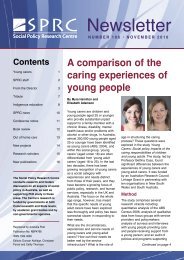
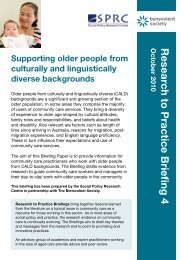
A visual example of the 1998 South Australian lifetable appears at Figure 1. It has a curve
typical of developed countries, with high survival until older ages. Males have death rates
higher than females from birth and this affects their surviving population, so that the male
survival curve is below that of the female.
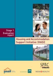
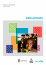
In Figure 2, the same 1998 life-table information is presented as deaths by single age,
rather than survivors, for these representative 100 000 populations. Here it can be seen
that, compared with female deaths, male infant deaths are higher, there is a rise in male
deaths in late teens, and deaths in older age begin to rise earlier for males. These
circumstances combine to give males a five-year reduction in the mean expectation of life
at birth compared to females. A formula that delivers more services to an increasingly
aged population size, as the current benchmark approach does, is a valuable and
accountable feature of the aged care program. Use of health services, however, is much
more closely related to time until death than time from birth (Fuchs 1984; van Weel and
Michels, 1997; Himsworth and Goldacre, 1999). One estimate is that health service
expenditure in the last year of life is 6.6 times (in the next to last year, 2.3 times) as large
as for those who survived at least two years (Fuchs, 1984). So aged care services may be
better targeted if based on years from death than years from birth, as is now the case.
5 Note this is the ‘current’ life table method. An alternative is the cohort life table method,
where the death rate experience of birth cohorts is used, see for example Armitage and
Berry, 1994: 470. Current life tables can also be produced for age groups and these are
referred to as abridged life tables. Life tables in this paper were produced by the Australian
Bureau of Statistics.
6 There are smoothing formulae applied in official tables to adjust for annual fluctuations. In
Australia that has meant using three years of data to produce life tables for the middle year.
157

BRIAN FLEMING
Figure 1: Lifetable Survival Curves, South Australia, Male and Female
100000
90000
80000
70000
60000
50000
40000
30000
20000
10000
Survivors
females
males
0
0 5 10 15 20 25 30 35 40 45 50 55 60 65 70 75 80 85 90 95 10
0
Age
10
5
11
0
Source: ABS, 1999, Catologue No. 3311.4
Figure 2: Lifetable Deaths Curves, South Australia, Male and Female
6000
5000
4000
3000
Deaths
females
males
2000
1000
0
1 6 11 16 21 26 31 36 41 46 51 56 61 66 71 76 81 86 91 96 10
1
Age
10
6
11
1
Source: ABS, 1999, Catalogue No. 3311.4
An approach based on years from death, or life expectancy, is supported by evidence that
the expected length of stay in residential aged care, in Australia, varies very little
compared with age at entry, see Table 1, (Australian Institute of Health and Welfare,
1999). Years to death is relatively constant at about one year for males and two years for
158

TARGETING AGED CARE TO PEOPLE WHO ARE DISADVANTAGED
females. If anything, the trend is that the younger the age at entry the shorter the length of
stay, contrary to what might be expected. 7
Table 1: Expected Length of Stay in Residential Care by Age, Compared with Life
Expectancy at that Age
Age ‘x’
Life expectancy at
age ‘x’
Expected length of stay
(years) at age ‘x’
Males 65 16.1 0.7
80 7.2 0.9
90 4.0 1.1
Females 65 19.8 1.9
80 9.0 2.2
90 4.6 2.1
Source: AIHW Australia’s Welfare 1999, Chapter 6; Gibson 1996.
Life Expectancy and Residential Aged Care
In this section I establish that information about the lifetable model of deaths offers a
reliable surrogate indicator for the pattern, by age, of entry to residential aged care.
The aim was to gain an understanding of relationships, between life expectancy and
residential care use. I obtained data from the Department of Health and Aged Care on the
current age, of all persons in residential aged care in South Australia, at 30 June 2000.
The age distribution of actual use of residential aged care in South Australia in June 2000
is shown in Figure 3 and Figure 4. Note that few people aged 70 years, the ‘planning age’,
use residential aged care. The median age at entry to residential care in South Australia is
about 82 years, so using the population 70+ includes the majority of people who use aged
care but the planning age itself is not a representative descriptor of the population using
aged care, in a statistical sense. This has led to suggestions that raising the planning age to
80+ years would make more sense, as this would be closer to the median age at entry and
an age more representative of the pattern of use – this idea is criticised later in the paper.
The lifetable deaths for South Australia, are the product of rising age-specific death rates
by age and a diminishing population by age. Similarly the population in aged care is a
product of rising age-specific risk of admission and a diminishing population by age. It is
likely that these are related as life expectancy in aged care is limited, see Table 1, and
most separations are due to death. Data on residents in aged care services were overlayed
with deaths data, and are discussed separately by sex.
For females the data were for current residents. According to Gibson, (see Table 1 1996,
5), female length of stay is about two years, independent of age. So, assuming an average
of one year in care for current female residents the deaths data were translated forward
7 While most departures will be due to death, this may be affected by transfers.
159

BRIAN FLEMING
one year so that the number of deaths relates to the age less one year. This puts the
‘deaths in two years’ data roughly in line with the resident data at entry to aged care, for
females. This results in Figure 4. The data are a very good visual match. Linear regresion
also confirms a very strong relationship: r-squared = 0.9623p

TARGETING AGED CARE TO PEOPLE WHO ARE DISADVANTAGED
In order to compare a years-from-death approach, with the current planning approach, the
South Australian lifetable was used to describe the pattern of survivors at aged 70 or
more. Given that the lifetable is based on current age-specific death rates, the shape of
this curve reflects the South Australian experience of survival at these ages; the actual
numbers are not relevant at this stage. It can be seen from Figure 5 that the current
method of counting the population aged 70 years or more is a poorer fit than deaths data,
r-squared = 0.3158, p70 1997-9 (schema life table)
and 2.residents (high and low care) 30 Jun 1999 (n=9612)
600
500
400
300
200
100
0
0 5 10 15 20 25 30 35 40 45 50 55 60 65 70 75 80 85 90 95 10
0
10
5
11
0
100000
90000
80000
70000
60000
50000
40000
30000
20000
10000
0
residents
survivors
Source: ABS (1999) Catalogue No. 3311.4
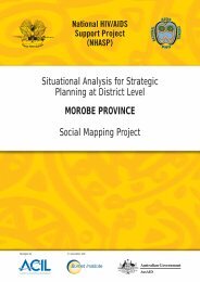
The exercise was repeated for data on males in residential care in South Australia,
without shifting the deaths data by one year. This is because the average length of stay is
only one year for males and the current age will already be roughly six months older than
age at entry (see Figure 6). The 70+ figure for males is similar to that of females but is not
shown; r-squared for deaths is 0.9285 p

BRIAN FLEMING
In Australia, and South Australia, a series of social atlases illustrate a variation of health
outcome by area, along with the spatial distribution of material and other resources, in
line with the expected pattern –the higher the material indicators the better the health
indicators, including mortality (Glover, Shand et al,. 1996; Glover and Tennant, 1999a
and 1999b).
Figure 6 The Distribution of Males in Residential Aged Care in South Australia by
Age, June 2000, and Deaths from South Australian Lifetable.
SA males by single age on two axes: 1. residents (high and low care) 30 Jun
2000 (n=3380) and 2. Deaths 1997-9 (life table n=100,000)
200
180
160
140
120
100
80
60
40
20
0
0 5 10 15 20 25 30 35 40 45 50 55 60 65 70 75 80 85 90 95 10
0
10
5
5900
4900
3900
2900
1900
900
-100
male residents
male deaths
If one area has lower life expectancy than another then its population will experience the
last two years of life at a lower age; the survivors at a given age will be fewer. So a
funding formula based on a particular age, say 70 years, will deliver greater resources to
areas that have a higher survival, other things, such as age structure, being equal.
For example, take two areas A and B with about a five-and-a-half year difference in life
expectancy; 81.5 and 75.9 years respectively. 8 Typical survival curves for the two areas
are shown at Figure 7. If the populations required care in the last two years of life, then on
average, population A would need care from 79.5 to 81.5 years and population B 74 to 76
years, with similar numbers of people requiring care. The population aged between 81
and 82 in Area A would be 62285 and between 79 and 80 in area B 62545. However,
under the present benchmark formula of 100/1000 70+, the difference in the suviving
population at age seventy is 85238 – 74697 = 10541. Under the benchmark formula for
aged care the Commonwealth would supply 8524 places in area A compared to 7470 in
area B, a difference of 1054 places.
8 This is about the size of the expected difference between the longest and shortest lived regions.
162

TARGETING AGED CARE TO PEOPLE WHO ARE DISADVANTAGED
Figure 7: Survival Curves for Two Populations Whose Life Expectancy is about 5
Years Different
Number surviving at
age x 100000
90000
80000
70000
60000
50000
40000
30000
20000
10000
0
Life Table survival curves
Life expectancy
at birth = 75.9
Survivors at
age = 70.0
Life expectancy
at birth = 81.5
x
Source ABS 3302.0
There are 11 South Australian planning regions, four metropolitan and seven nonmetropolitan,
used by the Commonwealth Department of Health and Aged Care. The four
metropolitan regions are, conveniently, North, South, East, and West. The consistent
overall pattern is that the East region experiences the best health and socioeconomic
circumstances, with the North the poorest, and West and South in between (Glover and
Woollacott, 1992). Life expectancy is therefore expected to reflect these general patterns.
However, regional and SLA life tables are not currently produced nationally. An
indication of what regional and SLA tables might reveal is given by some research in
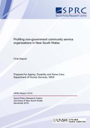
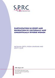
Victoria; a page extracted from the publication is at Figure 8. (Victoria, 1999, Burden of
Disease Study, http://www.dhs.vic.gov.au/phb/9903009/index) This shows the expected
regional variation in life expectancy, in this case for males by local government area. It
also shows a clustering of LGAs that are below, equal to or above the State averages,
particularly in the metropolitan area.
In the following pages I propose a method to distribute aged care resources using
information about the spatial distribution of life expectancy and show how it would
compare to the distribution based on the benchmark 100/1000 70+. In order to
demonstrate how a method based on deaths information might work, I have used median
age at death by SLA as a proxy measure for life expectancy. 9 The median age at death is
similar to life expectancy at birth, in most jurisdictions of Australia, but does not adjust
9 The ‘median age’ statistic does not standardise for the population structure, as life expectancy does,
and so will deliver a younger age where there is a younger age structure.
163

BRIAN FLEMING
Figure 8: Extract of Australian Example of Life Expectancy by Local Area
Source:Victoria, (1999) Burden of Disease
for age structure see Table 2 For example, younger age structures in the Northern
Territory and the ACT affect the size of the difference between life expectancy and
median age at death. 10 ABS supplied data on the average annual number of female
deaths, male deaths, male, female and person median age at death by SLA for the years
1997-99. 11 A wider range of years was not readily obtainable due to boundary changes.
Aggregates of those SLAs, however, were in current use in aged care planning aged care
through 1999.
10 The Northern Territory has a younger population and a relatively large indigenous population, which
has high standardised- mortality (2.2 for males and 1.5 females in 1997-98). The Australian Capital
Territory, the home of the national government, has a healthy, educated and young worker inmigration
effect.
11 SLAs were based on 1996 profiles.
164

TARGETING AGED CARE TO PEOPLE WHO ARE DISADVANTAGED
Table 2 Compare median age at death with expectation of life at birth, Australian
jurisdictions.
Median age death e 0 0 96/8 delta (LE-median)
Males Females Male Female Male Female
NSW 74.4 81 75.8 81.6 1.4 0.6
Vic 74.8 81.6 76.3 81.7 1.5 0.1
Qld 73.7 80.3 75.6 81.5 1.9 1.2
SA 75.3 81.7 76 81.6 0.7 -0.1
WA 73.6 80.8 76.1 81.9 2.5 1.1
Tas 75.1 80.5 75.1 80.4 0.0 -0.1
NT 53.7 57.7 70.6 75 16.9 17.3
ACT 72.6 78.8 77.5 81.6 4.9 2.8
Aust 74.3 81 75.9 81.5 1.6 0.5
Source: ABS, (1998:12) Table 1.1, 12 Catalogue No. 3302.0
Only SLAs with more than an average of 5 female deaths per year were used in the
subsequent analysis. 12 A scatter plot of median age at death by SLA appears at Figure 9.
Figure 9: Median Age at Death, Males, Females and Persons (ranked), by SLA
Median age at death, males, females, persons(ranked), by SLA deaths(f)>4
90.0
85.0
80.0
75.0
70.0
65.0
60.0
55.0
50.0
45.0
40.0
Persons
Males
Females
In Table 3, I have set out some basic features of the data. When separated into the
planning regions used by the Commonwealth, the metropolitan regions show the expected
relationship; the East has the highest group of median ages and the north the lowest, see
Figure 10.
12 The decision to use five deaths was based on discussion with ABS. Five female deaths was chosen as
the population in aged care is mainly female and it is a more conservative approach as male deaths
usually exceed female deaths.
165

BRIAN FLEMING
Table 3: Median Age at Death Data by SLA - Selected Features
SLA
Avg.
annual
male
deaths
Avg.
annual
female
deaths
Median
age death
male
Median
age death
female
Median
age death
persons
Lowest median age
at death persons 18 5.5 40.2 52.5 56.6
Highest median
age at death
persons 6 8 80.0 86.0 85.3
With most (male
and) female deaths 478.5 404.5 76.5 80.8 78.5
With largest
population
(111 910) 287 226.5 70.0 76.8 72.9
Figure 10: Median Age at Death, Persons, and Metropolitan Areas South Australia
(SLAs) Grouped into Commonwealth Planning Regions
Median age at death, deaths 1997-98, SLAs grouped into four urban planning regions, more than 5 female
deaths.
86.0
84.0
82.0
80.0
78.0
76.0
74.0
72.0
70.0
Gawler
T T Gully
Salisbury
Elizabeth
Munno
P
North
Glenelg Mitcham
Brighton
Onkaparing
Marion
Noarlunga
Happy
V ll
Willunga
South
West
THenley&Grang
Hindmarsh&Woodvill
Port
Ad l id
Thebarto
EnfieldB
West
Kensington
St Peters
Walkervill
Unley
Payneha
Adelaide
Burnside
East
Prospect
Cambelltow
Enfield
Stirling
East Torrens
Source: ABS (1999), Catalogue No. 3302.0
The non-metropolitan data is displayed at Figure 11.
166

TARGETING AGED CARE TO PEOPLE WHO ARE DISADVANTAGED
Figure 11: Median Age at Death, Persons, Non-metropolitan Areas South Australia
(SLAs) Grouped into Commonwealth Planning Regions
90.0
Median age at death, deaths 1997-98, SLAs grouped into seven non- urban
regions, more than 5 female deaths. Source ABS
85.0
80.0
75.0
70.0
Quorn
72.5
70.5
Cleve
80.9
Loxton 79.0
76.8 77.1
76.3
76.8 76.9 77.5 78.1
Berri
Tatiara
78.3
77.5
76.8
74.5
Mt Gambier
Tanunda
82.9
80.8 81.1 81.3
81.4 81.9
78.2 78.4 78.7 79.1 79.5
75.4
71.8 72.1
70.0
Mallala
Pinnaroo
80.9
80.1
78.3 78.9
77.3
76.2 76.3 76.4
74.4 75.0
Yankalilla
Orroroo
79.5
80.0
78.0
76.6 76.1
Pt Broughton
65.0
Ceduna
60.0
55.0
Uninc far north
Whyalla &
Far North Riverland Eyre South Yorke &
Hills
East
Barossa Mallee
Mid North
Source: ABS (1999), Catalogue No. 3302.0
In order to arrive at a representative median age at death by region the medians were
treated as means and population-weighted to arrive at the ‘medians’ in Table 4. I am well
aware of the arithmetical leap here but, while it would be a relatively straightforward
exercise for the ABS to make the calculations based on the original deaths data, it is
expensive for an individual to obtain this data, and not warranted as the exercise is
illustrative. The result is consistent with other spatial information and indicates clearly a
range of median age at death, by locality, for both Adelaide and the rest of South
Australia.
The analysis of deaths data and residents by age suggests that one possibility would be to
count the numbers of deaths and use the subsequent proportions by area to distribute aged
care. Note that the very strong correlation, between deaths data and resident data, is for
these two sets to move together by age. At SLA level, deaths are quite small in number,
and, while adequate to determine median age at death, are too unstable by single year to
discriminate well between SLAs for planning purposes. A surviving population measure
is more stable. What is needed is a distribution that matches the residential aged care
residents’ profile by SLA. The curve of survival above the life expectancy age is the
same shape as the last half of the curve of residents in aged care. If that last part of the
survival curve, by SLA, were mirrored about the vertical from the life expectancy age, the
resulting distribution would more closely match the residential distribution. This would
167

BRIAN FLEMING
Table 4: Median Age at Death, Persons, South Australian Areas (SLAs) Grouped
into Commonwealth Planning Regions
South Australian Region
Whyalla and far north Non-metropolitan 70.3
Riverland planning regions 76.3
Eyre 76.4
South East 76.6
Yorke &Barossa 77.4
Hills Mallee 77.4
Mid north
77.8
North Metropolitan regions 73.7
South 78.0
West 78.4
East
80.3
Median age at death
(yrs)
have the effect of doubling the population survival count at a given age. Since the
resulting count is to be used relatively, as it is distributional, the effect of doubling the
count and allocating proportions is the same as counting the original half and allocating
proportions.
ABS data was obtained on the population single ages from the 1996 census 13 . The
calculation is done for regions and the method is illustrated in Figure 12. Take the region
in the top row and the median age at death from the corresponding column in the second
row. The population greater than or equal to the median age at death is read from the first
column at the bottom of the table. The existing benchmark process reads the population
of each region from the 70+ row. So, for example for the northern metropolitan region,
the median age at death is 74 and the population is 9845, shown shaded in dark, rather
than the 70+ population of 15 410, unshaded.
A comparison of the proportion of places allocated to different regions using the
population over compared with the population older than the median age is shown at
Figure 13. The proportion of places that would ‘move’ is about 15 per cent; given 13 000
total places in South Australia, about 2 000 would move, summarised in Table 5.
13 ABS projected populations, for 1997-99, were only available in 5-year age groupings and
individual ages are necessary to plan at different ages. This is not important for the
comparison as the same population base is used, and individual age projections can be
sought from ABS.
168

TARGETING AGED CARE TO PEOPLE WHO ARE DISADVANTAGED
Figure 12: Determining the Population by Using a Life Expectancy Approach
Whyalla Yorke Lwr
Planning regionNorth South West East Eyre
Hills
Mallee
Flinders North
Mid NorthRiverlandSouth East Far NorthBarossa
Totals
Med age at
death - person
= 'X' 74 78 78 80 76 77 78 76 77 70 77
Population 'X' + 9845 13438 11030 12141 1521 4065 1302 1603 2292 3043 3684 63964
Region share
total based on
70+ pop 11.13% 22.78% 19.17% 22.81% 2.02% 6.31% 2.24% 2.25% 3.50% 2.20% 5.59% 1
Region share
based on
median age
"X"+ 15.39% 21.01% 17.24% 18.98% 2.38% 6.36% 2.04% 2.51% 3.58% 4.76% 5.76% 1
abs (med -70+) 4.26% 1.77% 1.93% 3.83% 0.35% 0.04% 0.20% 0.26% 0.08% 2.56% 0.17% 0.154688133
Population 65 + 24099 44037 36962 42721 4133 12711 4586 4610 7129 4881 11274
66+ 22208 41648 34927 40544 3842 11917 4277 4321 6658 4447 10534
67+ 20367 39199 32988 38290 3559 11085 3987 4032 6156 4099 9814
68+ 18671 36704 30899 36058 3298 10302 3686 3703 5710 3696 9110
69+ 17009 34134 28756 33886 3070 9524 3377 3410 5277 3362 8393
70+ 15410 31541 26547 31591 2802 8738 3101 3113 4850 3043 7734 138470
71+ 13887 29014 24294 29256 2573 7964 2824 2839 4422 2736 7020
72+ 12490 26566 22197 27096 2335 7220 2589 2612 4029 2469 6390
73+ 11128 24177 20038 24865 2122 6518 2315 2349 3657 2219 5841
74+ 9845 21734 18011 22703 1911 5874 2080 2078 3271 1954 5233
75+ 8631 19376 16033 20630 1727 5215 1870 1833 2943 1743 4704
76+ 7453 17095 14051 18591 1521 4645 1639 1603 2596 1520 4166
77+ 6341 15097 12319 16731 1370 4065 1452 1432 2292 1339 3684
78+ 5594 13438 11030 15198 1194 3611 1302 1266 2029 1186 3256
79+ 4876 11792 9754 13660 1052 3153 1140 1113 1778 1033 2866
80+ 4239 10223 8543 12141 916 2755 992 972 1548 861 2469
169

BRIAN FLEMING
Figure 13: Comparison of the Proportion of Aged Care Services by Region Using
Median Age at Death (+) versus 70 Years from Birth(+).
25.00%
Comparison between proportions of places by region using 70+ vs median age at death, SA planning
i
20.00%
15.00%
10.00%
5.00%
Sources
ABS data
1996 and 0.00%
1997/8
North South West East Eyre
Hills
Mallee
Mid North Riverland South
E t
Whyalla Yorke Lwr
Flinders North
Far North Barossa
70 + 11.13% 22.78% 19.17% 22.81% 2.02% 6.31% 2.24% 2.25% 3.50% 2.20% 5.59%
median age 15.39% 21.01% 17.24% 18.98% 2.38% 6.36% 2.04% 2.51% 3.58% 4.76% 5.76%
Source: ABS 1996 Census
Table 5: The Change in Service Distribution Using Median Age at Death
Pop 70+ Median age Change Absolute change
Percentages
North 11.13 14.10 2.97 2.97
South 22.78 24.66 1.88 1.88
West 19.17 15.93 -3.24 3.24
East 22.81 19.83 -2.98 2.98
Eyre 2.02 2.48 0.46 0.46
Hills Mallee 6.31 5.90 -0.41 0.41
Mid North 2.24 1.86 -0.38 0.38
Riverland 2.25 2.99 0.74 0.74
South East 3.50 3.74 0.24 0.24
Whyalla Flinders Far North 2.20 3.19 0.99 0.99
Yorke Lower North Barossa 5.59 5.32 -0.27 0.27
100.00% 0.00 14.56
The results are consistent with what one would expect from a distribution of services
based on life expectancy given the spatial segregation of South Australia shown in social
atlases (Glover, Shand et al., 1996; Glover and Tennant, 1999). The North Metropolitan
region ‘share’ of a given resource would rise, as the last two years of life would be
experienced at a younger age. The demonstration has been with median age, as a proxy
170

TARGETING AGED CARE TO PEOPLE WHO ARE DISADVANTAGED
for life expectancy, and so would distribute relatively more services to structurally
younger populations. A more sophisticated approach could be envisaged by calculating
male and female provision separately, based on a one- year expected residence for males
and two years for females, from Table 1. For policy purposes however, it may be
preferable to say simply that services are planned on known patterns of use.
It should be noted that, in South Australia, based on the current planning benchmark
100/1000 70+, there is a large ‘oversupply’ of places in the East region, a residential aged
care variant of the inverse care law. 14 Life expectancy, if calculated by region, or by
Statistical Local Area (SLA), uses deaths data and it is known that the calculation is
affected by the recorded ‘usual residence’ at death. So, if people from other regions, who
are likely to die younger, are unable to receive care, in the last two years of life, in their
home region and move to the East, to access the high supply, the life expectancy of the
East will reduce as an artefact. The effect will be to attenuate the differences between
regional life expectancy. So the method, if anything, will underestimate the size of the
redistribution required, at least at first.
Supporting Data on Actual Use
In the next section the theory, that there are spatial differences in the age at which
populations use aged care services, consistent with mortality experience, is confirmed in
two ways. One is that potential residents are assessed at different ages by region. Another
is that the actual use of residential aged care shows a variation of age by region.
Assessment
Assessment for entry to aged care is carried out independent of services by an Aged Care
Assessment Team (ACAT) in each planning region. The ACAT evaluation team report
shows a picture of assessments at higher ages in the east compared with other regions
(Basso, Pretreger et al., 1999: 22).
While the variation in age is small, it should be noted that ACATs assess for more than
residential aged care and the variation in age at assessment is consistent, for example,
with higher life expectancy in the east 15 .
The median age is higher than the mean age in each case indicating some skewness in
assessment age in the distribution.
14 ‘The availability of good medical care tends to vary inversely with the need for it in the population
served … This ... operates more completely where medical care is most exposed to market forces,
and less so where such exposure is reduced’ Hart, J. T. (1971), 405-12, 'Commentary: Three decades
of the inverse care law' Hart, 2000: 18-19.
15 A caution must be noted that this is assessment of eligibility for, not the same as admission to aged
care.
171

BRIAN FLEMING
Table 6: ACAT Client Age by Team(s) 1998
ACAT team(s) Median Mean
Northern 82 80.4
Western 82 80.6
Southern 83 81.8
Eastern 83 82.1
All Metropolitan 83 81.2
All Country 82 81.4
Source: ACAT Evaluation Unit Report Jan-Jun 1998.
Residential Aged Care
Data were obtained on the age at entry to residential aged care. A potential confounder is,
as noted above, that there is high supply in the East region and low supply in the North
region, against the benchmark. This means that the age of existing residents will not truly
reveal any pattern in the predicted direction, to the extent that younger residents move
from North to East to gain services. Accordingly, data were extracted on a cross section
of residents in permanent residential aged care at 31 December 2000 and divided into
regions based on the address recorded when the aged care assessment had been made.
The assessment form asks for ‘preferred contact address’ and it is possible that a
proportion of these will have the address of a friend or relative not in the same home
region as the resident. This is a limitation of the data collection. The results are shown in
Table 7 by sex, separately for metropolitan and non-metropolitan regions and ranked by
female mean age, females being the main users of residential aged care.
The age differences are notable. For comparison, a two-year difference in life expectancy
is the estimated impact of eliminating all cancer.
The use of contact address is unlikely to have an impact. There would have to be younger
aged care residents from higher socioeconomic areas systematically giving lower
socioeconomic area contact addresses, or older people from lower socioeconomic areas
systematically giving higher socioeconomic area contact addresses, for the result to be in
doubt. This may happen if the individual circumstances of the person were not that of the
area, the ecological fallacy, in which case the underlying association with socioeconomic
circumstances would, ironically, be confirmed. It seems more likely that the impact
would be to attenuate the real differences by younger people from lower socioeconomic
areas giving a higher socioeconomic area as the, say, child’s address.
Comparing The Ranking of Regions Using Median Age at Death and Age at Entry.
The ranking of the regions in Table 4 and Table 7 is similar, with an outlier of Eyre. The
median age at death of persons in Eyre is affected by the size of the indigenous population
relative to the non-indigenous population, with indigenous deaths at younger ages. The
172

TARGETING AGED CARE TO PEOPLE WHO ARE DISADVANTAGED
Table 7: Age at Admission by Region: SA Residents in Permanent Care by
Preferred Contact Address and Age at Date of Admissions: 31 December 2000
Ranked by female mean age.
Female
Male
Metro Mean Age Median Age Mean Age Median Age
MetroNorth 83.6 84 80.3 81
MetroWest 84.7 86 81.5 82
MetroSouth 85.3 86 82.3 83
MetroEast 85.4 87 81.5 83
Non-Metro
WhyallaFlindersFarNorth 81.4 83 78.8 80
Riverland 84.3 85 82.1 84
SouthEast 84.4 85 82.0 83
MidNorth 84.6 86 79.5 82
YorkeLwrNthBarossa 84.7 86 81.1 82
HillsMalleeSouthern 85.0 86 81.0 82
Eyre 87.4 88 80.3 81
residential aged care data are from non-indigenous providers obtained via the payments
system for standard, aged care services. Data were not obtained on the ages of people in
indigenous aged care programs in the Eyre region, which have a different funding
mechanism, where age is not recorded.
With Eyre excluded, the association between the rank of the planning region based on
median age at death (persons) and the rank of the region based on the mean female age at
entry to aged care is significant. 16 With Eyre included the rank correlation two tailed p=
0.117, and with Eyre excluded p = 0.009.
4 Discussion
This paper is not concerned with the overal quantum of places of aged care, rather their
distribution. Some caution would be necessary in the use of life expectancy for other than
16 Note that the deaths data were for persons as it is intended to use general population data as the
planning tool. The age at entry is for females, the main users of aged care.
173

BRIAN FLEMING
Table 8: The Ranking of South Australia Regions by Median Age at Death (Persons)
Compared with Age of Female Residents at Entry to Residential Care by Contract
Address
Including Eyre Excluding Eyre
Rank a Rank b Rank a Rank b
Whyalla, Flinders, Far North 1 1 1 1
North 2 2 2 2
Eyre 3 11
Riverland 4 3 3 3
Hills Mallee 5 8 4 8
South East 6 4 5 4
Yorke, Lower, North Barossa 7 6 6 6
South 8 9 7 9
West 9 7 8 7
Mid North 10 5 9 5
East 11 10 10 10
distributive effects. Life expectancy has increased since the 100/1000 70+ formula was
introduced in 1986, but the absolute period of life with a disability is either not changing
or may be slightly decreasing (Mathers and Robine 1998). 17 The disability-free years of
life are increasing, and increasing as a proportion of life, for disability requiring
residential care. People were not ‘sicker’ or more frail, for longer periods of their life, in
1997 than they were in 1985, when the formula was introduced. So if the formula,
100/1000 70+, described the ‘correct’ proportion of the 1985 population requiring
services, it now describes a greater proportion of the population, yet there is increasing
demand.
Table 9: Expectation of Life at Birth and at 65 Years: 1985 and 1997
c1985 1996-8
Expectation of life Male Female Male Female
At birth 71.2 78.2 75.86 81.52
At age 65 13.7 17.9 16.32 20.01
Source: ABS (1999), Catalogue No. 3302.0
Drivers of demand have had some scrutiny. High levels of personal care can be met by
committed and skilled carers, and carer support, or lack of it, is a critical factor in
admission to residential aged care, separate from clinical measures of the individual. Care
needs can be met at home; the majority of carers are spouses and the children of people
17 The compression of morbidity thesis was advanced by Fries in (1989: 205-28).
174

TARGETING AGED CARE TO PEOPLE WHO ARE DISADVANTAGED
entering aged care services are themselves nearing retirement ages (Gibson 1996). Gibson
and Liu (1995) suggest that structural ageing has an effect. This is to say that the need for
aged care increases with age, such that the portion of the population 80+ has a higher risk
of admission to aged care, and so an increasing proportion of people 80+ increases
demand, or ‘need’. This point was reiterated in an Australian Institute of Health and
Welfare (2000) paper on disability and ageing, which suggested a one in three chance of a
person over 65 years ever needing aged care compared with a population in aged care at
any one time aged 65 years being about three per cent (Australian Institute of Health and
Welfare 2000). However, it was acknowledged that this conclusion was drawn from
examining the existing population in residential care, and so could not be regarded as a
statement about any objective measure of need. It also did not take increases in life
expectancy into account. Gibson’s papers point to use of disability as a guide to demand,
but these measures are not available at SLA level so it is not yet feasible to use them for
these purposes
The fact that use of aged care services increases with age has contributed to calls for the
80+ population to be used as a better indicator of need. However, as has been
demonstrated, age-based formulae deliver a higher proportion of services to longer lived
populations, that is, to higher socioeconomic areas. The higher the age the greater that
distribution. To illustrate this effect, consider the following graph, Figure 14. It shows the
proportion of the metropolitan population above a particular age by region against the
proportion of the existing metropolitan aged care supply by region. The large movements
by age are in the North and East. The North share of population declines as the age
increases, and the East share rises. This is expected with lower life expectancy in the
North; the higher the age the fewer survivors. The aged care supply stays as horizontal
lines by age. The gap between the two lines is regarded as the ‘need’ - indicated by age, or
population share minus supply share. At lower ages the East supply substantially exceeds
population but this narrows as the age increases. In the North, supply is below population
at age 70+ but not at age 80+. A planning benchmark age of 80+ would see the current
distribution of supply as being appropriate, perversely, because there would be fewer
survivors in the North. 18 The main point from the graph is that the volatility of age based
planning makes it a poor indicator of need.
Certain conditions associated with residential aged care use may not be consistent with
planning based on mortality. The prevalence of dementia increases with age, and there
may not be as strong an association of that condition with socioeconomic circumstances
as there is of mortality. However, life expectancy with dementia, beyond age 65, for both
18 Note this is not adjusted for any cohort settlement effects.
175

BRIAN FLEMING
Figure 14: The Regional Proportion of the Metropolitan Population Above Ages
Compared with the Regional Proportion of Metropolitan Aged Care Supply in
South Australia
0.4
0.35
0.3
0.25
0.2
0.15
0.1
0.05
Eastern
Northern
Southern
Western
Eastern supply
Northern supply
Southern supply
Western supply
0
Sum of P65+ Sum of P70+ Sum of P80+ Sum of P85+
Source: ABS (middle projection of year 2001 population) and Department of Health and
Aged Care Supply tables 31 January 2001
sexes, has been estimated at one year, so the condition is feeding in to lifetables via agespecific
death rates (Ritchie 1994).
The current planning method, based on years from birth, also distributes services to areas
that were settled at particular times. As Australia’s population expanded, particularly over
the last 50 years, with post World War II migration, new housing areas were established
from greenfields. If, for example, most people settled in an area in 1955, when they were
25, they will turn 70 together in 2000 and be counted for planning purposes, while not
having the age distribution of longer settled areas. Planning based on mortality would
overcome this weakness.
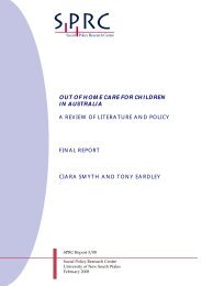
There is a spatial distribution of the sex ratio, the number of males to 100 females. In
metropolitan areas the number of females 65+ outnumbers males but this reverses in
remote and some rual regions in Australia (Haberkorn, Hugo et al. 1999, 116). This is
illustrated in Figure 15. Since men die younger than women, a fixed planning age delivers
more services to longer lived women and therefore disadvantages remote Australia for
aged care services, albeit at low numbers. Planning based on life expectancy would
incorporate adjustments for such populations.
176

TARGETING AGED CARE TO PEOPLE WHO ARE DISADVANTAGED
Figure 15 Sex Ratio, Australia Population 65+, 1996
Source: National Key Centre for Social Applications of GIS
5 Conclusion
The social gradient in health persists into old age, and there is a clear social gradient in
age at death. There is a spatial distribution of socioeconomic circumstances and therefore
of life expectancy. An age-based planning mechanism, that is, years from birth, therefore
distributes finite resources spatially to longer lived populations. Perversely, the older the
planning age, the greater the distribution of services would be to higher socioeconomic
areas. Choosing a planning age closer to the median age at entry to aged care services, say
80 years or more, an apparently more meaningful age statistically, would have a
distributive effect towards higher socioeconomic areas. 19
19 There are also cohort effects of areas settled at particular times.
177

BRIAN FLEMING
Aged care legislation includes the capacity to consider financial or social disadvantage
and there are no current mechanisms to address this special needs group. An approach
based on life expectancy, such as years to death or equal probability of death would better
predict the distributed use of residential aged care services. It would therefore better target
aged care resources.
There may be other distributive advantages. A life expectancy method can be applied to
particular populations other than spatially. So, for example, there need not be a different
planning approach to distributing services for indigenous populations. 20 Similarly for
rural areas, as the method adjusts for the sex ratio change that is experienced by remote
Australia, given the lower life expectancy of males. The method also adjusts for different
age structures.
The method requires the calculation of life tables by region and SLA and populations
projected by single age. While these are not routinely available, they do not require any
additional data collection by the ABS to be produced. Home address mobility, a potential
problem for such calculations, is lowest at age 65 years (Bell and Hugo 2000: 172).
Data on the age structure of persons in residential aged care confirms a spatial pattern of
use of aged care services consistent with the association between the expectation of life
and socioeconomic circumstances.
References
Armitage, P. and G. Berry (1994). Statistical Methods in Medical Research. Blackwell
Science Ltd, Oxford.
Australian Bureau of Statistics (ABS) (1999), Demography, South Australia, Catalogue
No. 3311.4, ABS, Canberra
Australian Bureau of Statistics (ABS) (1999), Deaths, Australia, Catalogue No. 3302.0
ABS, Australia.
Australian Institute of Health and Welfare (1999), Australia's Health 1999, Australian
Institute of Health and Welfare, Canberra.
Australian Institute of Health and Welfare (2000), Disability and Ageing: Australian
Population Patterns and Implications, Australian Institute of Health and Welfare,
Canberra
Basso, P., L. Pretreger et al. (1999), Aged Care Assessment Program South Australia
Evaluation Unit Report, Department of Human Services, South Australia, Adelaide.
Bell, M. and G. Hugo (2000), Internal Migration in Australia 1991-1996, Australian
Population, Immigration and Multicultural Research Program, Commonwealth of
Australia, Canberra.
20 Tacit acceptance of planning for aged care bearing some relationship to life expectancy has been the
different planning age used by the Commonwealth for Aboriginal and Torres Strait Islander
populations, that is, the population aged 50+ rather than 70+.
178

TARGETING AGED CARE TO PEOPLE WHO ARE DISADVANTAGED
Commonwealth of Australia (1986), Nursing Homes and Hostels Review, Department of
Community Services and Health, Canberra.
Fries, J. F. (1989), 'The compression of morbidity: near or far?, The Milbank Quarterly,
67 (2): 208-28.
Fuchs, V. R. (1984), '"Though much is taken": reflections on ageing, health, and medical
care', Milbank Memorial Fund Quarterly/Health and Society, 62 (2), 143-67.
Gibson, D. (1996), 'Reforming aged care in Australia: change and consequence', Journal
of Social Policy, 2, 157–79.
Gibson, D. and Z. Liu (1995), 'Planning ratios and population growth: will there be a
shortfall in residential aged care by 2021?' Australian Journal on Ageing, 14 (2),
57-62.
Glover, J., M. Shand, et al. (1996), A social health atlas of South Australia, South
Australian Health Commission, Commonwealth of Australia, Adelaide,.
Glover, J. and S. Tennant (1999a), A Social Health Atlas of Australia, Public Health
Information Development Unit, Commonwealth of Australia, Adelaide.
Glover, J. and S. Tennant (1999b), A Social Health Atlas of Australia, Public Health
Information Development Unit, Commonwealth of Australia, Canberra.
Glover, J. and T. Woollacott (1992), A Social Health Atlas of Australia, Commonwealth
of Australia, Adelaide.
Haberkorn, G., G. Hugo et al. (1999), Country Matters Social Atlas of Rural and
Regional Australia, Commonwealth of Australia Bureau of Rural Sciences,
Canberra.
Hart, J. T. (1971), 'The inverse care law', Lancet, i, 405-12.
Hart, J. T. (2000), 'Commentary: three decades of the inverse care law' British Medical
Care Journal, 320, 1 January, 18-19.
Himsworth, R. L. and M. J. Goldacre (1999), 'Does time spent in hospital in the final 15
years of life increase with age at death? A population based study', British Medical
Journal, 319, November, 1338-39.
Mathers, C. D. and J. M. Robine (1998), 'International trends in health expectancies: a
review', Australasian Journal on Ageing, 17, 1 Supplement, 51-5.
Ritchie, K. (1994), International comparisons of dementia-free life expectancy: a critical
review of the results obtained, Advances in Health Expectancies, Australian
Institute of Health and Welfare, Canberra.
van Weel, C. and J. Michels (1997), 'Dying, not old age, to blame for costs of health care',
Lancet, 350 (9085) 1159-60.
Victoria (1999), Burden of Disability Study,
http://www.dhs.vic.gov.au/phb/9903009/index
179