Fisher information matrix for Gaussian and categorical distributions
Fisher information matrix for Gaussian and categorical distributions
Fisher information matrix for Gaussian and categorical distributions

Create successful ePaper yourself
Turn your PDF publications into a flip-book with our unique Google optimized e-Paper software.
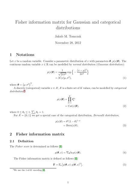
<strong>Fisher</strong> <strong>in<strong>for</strong>mation</strong> <strong>matrix</strong> <strong>for</strong> <strong>Gaussian</strong> <strong>and</strong> <strong>categorical</strong><br />
<strong>distributions</strong><br />
Jakub M. Tomczak<br />
November 28, 2012<br />
1 Notations<br />
Let x be a r<strong>and</strong>om variable. Consider a parametric distribution of x with parameters θ, p(x|θ). The<br />
contiuous r<strong>and</strong>om variable x ∈ R can be modelled by normal distribution (<strong>Gaussian</strong> distribution):<br />
1<br />
{<br />
p(x|θ) = √ exp (x −<br />
}<br />
µ)2<br />
−<br />
2πσ<br />
2 2σ 2<br />
= N (x|µ, σ 2 ), (1)<br />
where θ = ( µ σ 2) T<br />
.<br />
A discrete (<strong>categorical</strong>) variable x ∈ X , X is a finite set of K values, can be modelled by <strong>categorical</strong><br />
distribution: 1 p(x|θ) =<br />
K∏<br />
k=1<br />
θ x k<br />
k<br />
= Cat(x|θ), (2)<br />
where 0 ≤ θ k ≤ 1, ∑ k θ k = 1.<br />
For X = {0, 1} we get a special case of the <strong>categorical</strong> distribution, Bernoulli distribution,<br />
2 <strong>Fisher</strong> <strong>in<strong>for</strong>mation</strong> <strong>matrix</strong><br />
2.1 Definition<br />
The <strong>Fisher</strong> score is determined as follows [1]:<br />
p(x|θ) = θ x (1 − θ) 1−x<br />
The <strong>Fisher</strong> <strong>in<strong>for</strong>mation</strong> <strong>matrix</strong> is defined as follows [1]:<br />
1 We use the 1-of-K encoding [1].<br />
= Bern(x|θ). (3)<br />
g(θ, x) = ∇ θ ln p(x|θ). (4)<br />
F = E x<br />
[<br />
g(θ, x) g(θ, x)<br />
T ] . (5)<br />
1
2.2 Example 1: Bernoulli distribution<br />
Let us calculate the fisher <strong>matrix</strong> <strong>for</strong> Bernoulli distribution (3). First, we need to take the logarithm:<br />
Second, we need to calculate the derivative:<br />
ln Bern(x|θ) = x ln θ + (1 − x) ln(1 − θ). (6)<br />
d<br />
dθ ln Bern(x|θ) = x θ − 1 − x<br />
1 − θ<br />
= x − θ<br />
θ(1 − θ) . (7)<br />
Hence, we get the following <strong>Fisher</strong> score <strong>for</strong> the Bernoulli distribution:<br />
g(θ, x) =<br />
x − θ<br />
θ(1 − θ) . (8)<br />
The <strong>Fisher</strong> <strong>in<strong>for</strong>mation</strong> <strong>matrix</strong> (here it is a scalar) <strong>for</strong> the Bernoulli distribution is as follows:<br />
F = E x [g(θ, x) g(θ, x)]<br />
[ (x − θ)<br />
2 ]<br />
= E x<br />
(θ(1 − θ)) 2<br />
=<br />
=<br />
=<br />
=<br />
=<br />
1<br />
{<br />
E<br />
(θ(1 − θ)) 2 x [x 2 − 2xθ + θ 2 ]<br />
1<br />
{<br />
}<br />
E<br />
(θ(1 − θ)) 2 x [x 2 ] − 2θE x [x] + θ 2<br />
1<br />
{<br />
}<br />
θ − 2θ 2 + θ 2<br />
(θ(1 − θ)) 2<br />
2.3 Example 2: Categorical distribution<br />
}<br />
1<br />
θ(1 − θ)<br />
(θ(1 − θ))<br />
2<br />
1<br />
θ(1 − θ) . (9)<br />
Let us calculate the fisher <strong>matrix</strong> <strong>for</strong> <strong>categorical</strong> distribution (2). First, we need to take the logarithm:<br />
ln Cat(x|θ) =<br />
Second, we need to calculate partial derivatives:<br />
K∑<br />
x k ln θ k . (10)<br />
k=1<br />
∂<br />
∂θ k<br />
ln Cat(x|θ) = x k<br />
θ k<br />
. (11)<br />
Hence, we get the following <strong>Fisher</strong> score <strong>for</strong> the <strong>categorical</strong> distribution:<br />
⎡<br />
⎢<br />
g(θ, x) = ⎣<br />
x 1<br />
⎤<br />
θ ḳ<br />
.<br />
x K<br />
θK<br />
⎥<br />
⎦ . (12)<br />
2
Now, let us calculate the product of <strong>Fisher</strong> score <strong>and</strong> its transposition:<br />
⎡(<br />
)<br />
⎡<br />
x 1<br />
⎤<br />
2<br />
⎤<br />
x 1 x 1 x 2<br />
x<br />
θ ḳ<br />
⎢ ⎥<br />
⎣ . ⎦ [ x 1 x<br />
θ k<br />
· · · K<br />
] θ 1 θ 1 θ 2<br />
· · · 1 x K<br />
θ 1 θ K<br />
θK = ⎢<br />
x K<br />
⎣<br />
. . · · · . ⎥<br />
( ) 2<br />
⎦<br />
θK<br />
x K x 1 x K x 2<br />
x<br />
θ K θ 1 θ K θ 2<br />
· · · K<br />
θK<br />
⎡<br />
⎤<br />
g 11 g 12 · · · g 1K<br />
⎢<br />
⎥<br />
= ⎣ . . · · · . ⎦ . (13)<br />
g K1 g K2 · · · g KK<br />
There<strong>for</strong>e, <strong>for</strong> g kk we have:<br />
E x [g kk ] = E x<br />
[( xk<br />
θ k<br />
) 2 ]<br />
= 1 θ 2 k<br />
E x [x 2 ]<br />
= 1 θ k<br />
, (14)<br />
<strong>and</strong> <strong>for</strong> g ij , i ≠ j:<br />
Finally, we get:<br />
E x [g ij ] = E x<br />
[ xi x j<br />
θ i θ j<br />
]<br />
= 1<br />
θ i θ j<br />
E x [x i x j ]<br />
= 0. (15)<br />
F = diag{ 1<br />
θ 1<br />
, . . . ,<br />
1<br />
}<br />
. (16)<br />
θ K<br />
2.4 Example 3: Normal distribution<br />
Let us calculate the <strong>Fisher</strong> <strong>matrix</strong> <strong>for</strong> univariate normal distribution (1). First, we need to take the<br />
logarithm:<br />
ln N (x|µ, σ 2 ) = − 1 2 ln 2π − 1 2 ln σ2 − 1<br />
2σ 2 (x − µ)2 . (17)<br />
Second, we need to calculate the partial derivatives:<br />
∂<br />
∂µ N (x|µ, σ2 ) = 1 (x − µ)<br />
σ2 (18)<br />
∂<br />
∂σ N (x|µ, 2 σ2 ) = − 1<br />
2σ + 1<br />
2 2σ (x − 4 µ)2 . (19)<br />
Hence, we get the following <strong>Fisher</strong> score <strong>for</strong> normal distribution:<br />
[ ∂<br />
g(θ, x) =<br />
N (x|µ, ]<br />
∂µ σ2 )<br />
∂<br />
N (x|µ, σ 2 )<br />
∂σ<br />
[<br />
2 ]<br />
1<br />
(x − µ)<br />
=<br />
σ 2<br />
− 1 + 1 (x − µ) 2 . (20)<br />
2σ 2 2σ 4<br />
3
Now, let us calculate the product of <strong>Fisher</strong> score <strong>and</strong> its transposition:<br />
⎡<br />
⎤<br />
1<br />
(x − µ)<br />
σ<br />
⎣<br />
2 ⎦ [ 1<br />
(x − µ) − 1 + 1 (x − µ) 2] =<br />
− 1 + 1 (x − µ) 2 σ 2 2σ 2 2σ 4<br />
2σ 2 2σ 4<br />
⎡<br />
⎤<br />
1<br />
(x − µ) 2 − 1 (x − µ) + 1 (x − µ) 3<br />
σ<br />
⎣<br />
4 2σ 4 2σ 6 ⎦ = (21)<br />
− 1 (x − µ) + 1 (x − µ) 3 1 − 1 (x − µ) 2 + 1 (x − µ) 4 2σ 4 2σ 6 4σ 4 2σ 6 4σ<br />
⎡ ⎤<br />
8<br />
g 11 g 12<br />
⎣ ⎦ ,<br />
g 22<br />
g 21<br />
where g 12 = g 21 .<br />
In order to calculate the <strong>Fisher</strong> <strong>in<strong>for</strong>mation</strong> <strong>matrix</strong> we need to determine the expected value of<br />
all g ij . Hence, 2 <strong>for</strong> g 11 :<br />
<strong>and</strong> <strong>for</strong> g 12 :<br />
<strong>and</strong> <strong>for</strong> g 22 :<br />
E x [g 11 ] = E x<br />
( 1<br />
σ 4 (x − µ)2 )<br />
= 1 σ 2 (<br />
Ex [x 2 ] − 2µ 2 + µ 2)<br />
= 1 σ 2 (<br />
µ 2 + σ 2 − 2µ 2 + µ 2)<br />
= 1 σ 2 , (22)<br />
(<br />
E x [g 12 ] = E x − 1<br />
1<br />
)<br />
(x − µ) +<br />
2σ4 2σ (x − 6 µ)3<br />
= − 1<br />
( 1<br />
2σ (E x[x] − µ) + E 4 x<br />
)<br />
2σ 6 (x3 − 3x 2 µ + 3xµ 2 − µ 3 )<br />
)<br />
= 1<br />
2σ 6 (<br />
(E x [x 3 ] − 3µE x [x 2 ] + 3µ 2 E x [x] − µ 3 )<br />
E x [g 22 ] = E x<br />
( 1<br />
4σ 4 − 1<br />
2σ 6 (x − µ)2 + 1<br />
4σ 8 (x − µ)4 )<br />
= 1<br />
2σ 6 ( (µ 3 + 3µσ 2 − 3µ(µ 2 + σ 2 ) + 3µ 3 − µ 3))<br />
= 0, (23)<br />
= 1<br />
4σ 4 − 1<br />
2σ 6 E x[x 2 − 2xµ + µ 2 ] + 1<br />
4σ 8 E x[x 4 − 4x 3 µ + 6x 2 µ 2 − 4xµ 3 + µ 4 ]<br />
= 1<br />
4σ 4 − 1<br />
2σ 6 (<br />
E x [x 2 ] − 2E x [x]µ + µ 2 )<br />
+ 1<br />
4σ 8 (<br />
E x [x 4 ] − 4E x [x 3 ]µ + 6E x [x 2 ]µ 2 − 4E x [x]µ 3 + µ 4 )<br />
= 1<br />
4σ 4 − 1<br />
2σ 6 σ2 + 1<br />
4σ 8 3σ4<br />
= 1<br />
2σ 4 . (24)<br />
Finally, we get:<br />
F =<br />
2 See Section 3 <strong>for</strong> raw moments of univariate normal distribution.<br />
[ 1<br />
]<br />
0<br />
σ 2 1 . (25)<br />
0<br />
2σ 4<br />
4
2.5 Summary<br />
The <strong>Fisher</strong> <strong>in<strong>for</strong>mation</strong> <strong>matrix</strong> <strong>for</strong> given distribution:<br />
• Bernoulli distribution:<br />
• Categorical distribution:<br />
• Normal distribution:<br />
F =<br />
1<br />
θ(1 − θ) ,<br />
F = diag{ 1<br />
θ 1<br />
, . . . ,<br />
F =<br />
[ 1<br />
]<br />
0<br />
σ 2 1 .<br />
0<br />
2σ 4<br />
1<br />
}<br />
,<br />
θ K<br />
3 Appendix: Raw moments<br />
Table 1: The raw moments of univariate normal distribution.<br />
Order Expression Raw moment<br />
1 E x [x] µ<br />
2 E x [x 2 ] µ 2 + σ 2<br />
3 E x [x 3 ] µ 3 + 3µσ 2<br />
4 E x [x 4 ] µ 4 + 6µ 2 σ 2 + 3µ 4<br />
References<br />
[1] C. Bishop. Pattern Recognition <strong>and</strong> Machine Learning. Springer, 2006.<br />
5