Grand Challenges in Ocean and Climate Modelling - STFC's ...
Grand Challenges in Ocean and Climate Modelling - STFC's ...
Grand Challenges in Ocean and Climate Modelling - STFC's ...

Create successful ePaper yourself
Turn your PDF publications into a flip-book with our unique Google optimized e-Paper software.
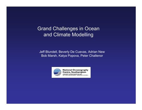
<strong>Gr<strong>and</strong></strong> <strong>Challenges</strong> <strong>in</strong> <strong>Ocean</strong><br />
<strong>and</strong> <strong>Climate</strong> Modell<strong>in</strong>g<br />
Jeff Blundell, Beverly De Cuevas, Adrian New<br />
Bob Marsh, Katya Popova, Peter Challenor
Challenge 1: Mix<strong>in</strong>g <strong>and</strong> Internal Waves<br />
The realistic representation of mix<strong>in</strong>g <strong>in</strong> ocean models is perhaps<br />
the biggest challenge fac<strong>in</strong>g physical oceanographers today<br />
1 cm 2 s -1<br />
0.1 cm 2 s -1<br />
This plot of zonal-mean vertical diffusivity (mix<strong>in</strong>g rate) from the OCCAM 1/12° model<br />
shows large diffusivities <strong>in</strong> the deep ocean, but the model does not resolve key processes,<br />
<strong>in</strong> particular <strong>in</strong>ternal waves.
Internal Wave Processes<br />
Internal waves are generated through the <strong>in</strong>teraction of surface tides (from the<br />
sun <strong>and</strong> moon) with topography, particularly steep shelf-slope<br />
topography <strong>and</strong> “rough” mid-ocean ridge topography <strong>in</strong> the deep ocean.<br />
Internal waves are an important mix<strong>in</strong>g process <strong>in</strong> the ocean but occur with<br />
length scales of typically a few km, so cannot be explicitly resolved <strong>in</strong><br />
today’s ocean models (i.e. the OCCAM 1/12° model has a resolution of<br />
order 10km horizontally).
Shelf Slope Generated Internal Waves (Bay of Biscay)<br />
Displacements<br />
Horizontal<br />
velocity<br />
Internal tides are order 30-50 km<br />
wavelength <strong>and</strong> are generated<br />
near the shelf break. They break<br />
down <strong>in</strong>to shorter 1-2 km <strong>in</strong>ternal<br />
waves shown here, through<br />
nonl<strong>in</strong>ear processes.<br />
Vertical<br />
velocity
Mix<strong>in</strong>g near the Shelf Break (Bay of Biscay)<br />
Surface chlorophyll on 4.9.99<br />
The <strong>in</strong>ternal tides <strong>and</strong> waves<br />
produce mix<strong>in</strong>g of the upper<br />
ocean near the shelf break.<br />
This <strong>in</strong>jects nutrients <strong>in</strong>to the<br />
well-lit layers <strong>and</strong> allows<br />
plant cells (phytoplankton/<br />
chlorophyll) to grow or<br />
“bloom” near the shelf break<br />
(200 m contour). So <strong>in</strong>ternal<br />
wave mix<strong>in</strong>g is important for<br />
biological growth <strong>in</strong> the<br />
ocean.
Internal Wave Mix<strong>in</strong>g <strong>in</strong> the Deep <strong>Ocean</strong><br />
Internal waves are thought to<br />
provide an important mix<strong>in</strong>g mechanism<br />
for stirr<strong>in</strong>g the deep ocean <strong>and</strong> upwell<strong>in</strong>g<br />
the deep waters to nearer the surface.<br />
This is an important route whereby waters<br />
which have left the surface can “overturn”<br />
<strong>and</strong> once more return to the surface. The<br />
mix<strong>in</strong>g is therefore critical to ma<strong>in</strong>ta<strong>in</strong><strong>in</strong>g the<br />
large-scale circulation <strong>in</strong> the ocean.<br />
The figure (from theory) shows that <strong>in</strong>ternal<br />
tides <strong>and</strong> waves provide 0.9 TW of energy<br />
to the deep ocean, nearly half of the total<br />
required (the rema<strong>in</strong>der be<strong>in</strong>g provided by<br />
the w<strong>in</strong>d).<br />
From Munk & Wunsch (1998)
Example from the Indian <strong>Ocean</strong>: Mascarene Plateau<br />
The topography west of the<br />
Plateau is relatively smooth<br />
<strong>and</strong> flat <strong>and</strong> does not produce<br />
<strong>in</strong>ternal waves.<br />
East of the Plateau the<br />
seafloor is highly canyonated<br />
due to the central Indian Ridge.<br />
The canyons (features runn<strong>in</strong>g<br />
NE to SW) are typically<br />
10-20 km across.
Mean Temperature Profiles<br />
The mean temperature profile East of the Plateau looks like a “mixed” version of the<br />
profile from West of the Plateau - as if <strong>in</strong>ternal waves were mix<strong>in</strong>g the deeper colder<br />
waters with lighter waters from above - upwell<strong>in</strong>g them several thous<strong>and</strong> metres.
Inferred Vertical Diffusivities (Mix<strong>in</strong>g Rates)<br />
Method of Polz<strong>in</strong> (1995) us<strong>in</strong>g ‘stra<strong>in</strong>’ (small scale variations <strong>in</strong> the vertical density gradient)<br />
<strong>in</strong>ferred from CTD measurements shows that mix<strong>in</strong>g is actually much<br />
higher East of the Plateau than West of it.<br />
Central<br />
West<br />
East<br />
K ρ ~ 10 -5 -10 -2<br />
m 2 s -1
Diffusivities over “Rough” Topography East of Mascarene Plateau<br />
Central<br />
West<br />
East<br />
In particular, diffusivities<br />
are much higher<br />
<strong>in</strong> topographic troughs or<br />
canyons than on ridges/<br />
crests.<br />
(The plots show mix<strong>in</strong>g<br />
estimates from 5 or 6<br />
“dips” with the CTD at each<br />
of two stations).<br />
Note the roughness of the<br />
topography - typical scales<br />
of 10-20 km.
Internal Waves at Station 17 (Trough)<br />
Internal waves of tidal period (<strong>and</strong> likely wavelengths of 10-20 km) are<br />
found above the rough topography (right-h<strong>and</strong> figure) <strong>and</strong> appear to be<br />
break<strong>in</strong>g <strong>in</strong> the canyons/ troughs (below 3500 m). The break<strong>in</strong>g of the waves is<br />
caus<strong>in</strong>g the mix<strong>in</strong>g of the deep ocean, <strong>and</strong> the upwell<strong>in</strong>g of the deep waters.
NEMO 1/4° global ocean model surface temperature<br />
Thus a global ocean model of order 1 km horizontal resolution would explicitly<br />
resolve a good part of the <strong>in</strong>ternal wave spectrum. The result<strong>in</strong>g mix<strong>in</strong>g could then<br />
be easily <strong>in</strong>cluded through (for example) a Richardson number dependent scheme.<br />
Improved parameterisations could also be developed for lower resolution models.<br />
This would be likely to cause a major change <strong>in</strong> the deep circulation patterns <strong>in</strong><br />
the global ocean, <strong>and</strong> <strong>in</strong> the upwell<strong>in</strong>g of the deep waters, <strong>and</strong> <strong>in</strong> the way <strong>in</strong> which<br />
the ocean circulation is ma<strong>in</strong>ta<strong>in</strong>ed. Such a model would therefore lead to major<br />
improvements <strong>in</strong> ocean <strong>and</strong> climate modell<strong>in</strong>g systems <strong>and</strong> predictions, <strong>and</strong> to<br />
our underst<strong>and</strong><strong>in</strong>g of how the ocean works.
Challenge 2: Global Carbon Cycle<br />
MesoZoo<br />
MicroZoo<br />
Diatoms<br />
NanoPhyto<br />
Si<br />
Fe<br />
N<br />
Slow<br />
detritus<br />
Fast particle<br />
flux<br />
Medusa: Model of Ecosystem Dynamics,<br />
nutrient Utilisation <strong>and</strong> SequestrAtion<br />
Chlorophyll from Medusa ecosystem model<br />
<strong>in</strong> global NEMO 1/4° model<br />
Models of upper ocean biology (eg the “Medusa” model at NOCS) can be easily built <strong>in</strong>to<br />
st<strong>and</strong>ard ocean models, eg the 1/4° NEMO model above. Upper ocean biology quickly comes<br />
<strong>in</strong>to a near-equilibrium, after less than a decade at most. It drives a carbon s<strong>in</strong>k<strong>in</strong>g flux or<br />
“pump” to the deeper ocean (a simple modification to Medusa would be needed for this),<br />
remov<strong>in</strong>g it from the atmosphere. However, it would take order 1000 years for the carbon <strong>in</strong> the<br />
deep ocean to come <strong>in</strong>to equilibrium (a typical “overturn<strong>in</strong>g” timescale for the ocean).<br />
Equilibration of the ocean carbon system is needed for a pre-<strong>in</strong>dustrial atmospheric CO2 level<br />
before studies can be made of how this “carbon pump” will change <strong>in</strong> the future <strong>and</strong> its role <strong>in</strong><br />
slow<strong>in</strong>g climate change. To date, this has only been achieved <strong>in</strong> models with 2° resolution.<br />
However, a 1/4° or 1/12° resolution is needed to adequately model the <strong>in</strong>teractions of eddies<br />
(which affect mixed layer depth <strong>and</strong> upwell<strong>in</strong>g of nutrients) with the biology.
Challenge 3: <strong>Climate</strong> Uncerta<strong>in</strong>ty<br />
AMOC simulated with GENIE-1<br />
(Marsh et al., 2007)<br />
How the climate will change <strong>in</strong> the future is far from certa<strong>in</strong>. For a particular<br />
model, different outcomes will be obta<strong>in</strong>ed for different parameter sett<strong>in</strong>gs <strong>in</strong><br />
the model (“parameter uncerta<strong>in</strong>ty”). The figure shows how the Atlantic<br />
Meridional Overturn<strong>in</strong>g Circulation (AMOC) might change <strong>in</strong> the future (for a<br />
given warm<strong>in</strong>g scenario) <strong>in</strong> the GENIE model, depend<strong>in</strong>g on how various<br />
parameters <strong>in</strong> the model are chosen. To properly assess the model’s<br />
response, about 10,000 – 100,000 runs would be needed to span the<br />
parameter space us<strong>in</strong>g naïve Monte Carlo methods.
Challenge 3: <strong>Climate</strong> Uncerta<strong>in</strong>ty<br />
Future AMOC simulated with<br />
GENIE-1<br />
(Challenor et al., 2008)<br />
If we build an “emulator” (a statistical approximation to the full climate model) we can reduce this number of<br />
runs to 0(100 - 1000) we can now apply statistical techniques, so that the probability of the collapse of the<br />
AMOC (for <strong>in</strong>stance) can be derived. (Such methods are be<strong>in</strong>g developed <strong>in</strong> the “Manag<strong>in</strong>g Uncerta<strong>in</strong>ty <strong>in</strong><br />
Complex Models” project, to m<strong>in</strong>imise the number of runs we do).<br />
For GENIE, the probability of AMOC collapse (with drastic implications for cool<strong>in</strong>g of European climate<br />
<strong>in</strong> the future) was estimated at about 30% (Challenor et al., 2006). However, GENIE has simplified physics<br />
(e.g. planetary geostrophic ocean) <strong>and</strong> a coarse resolution (3-10°, 8 ocean depth levels). The exercise should<br />
now be repeated for higher resolution full-physics GCMs which <strong>in</strong>clude more of the relevant processes. Such<br />
models have order 100 uncerta<strong>in</strong> parameters so our tra<strong>in</strong><strong>in</strong>g ensemble will need to be bigger.
Summary <strong>and</strong> Requirements<br />
Challenge 1: Internal Wave Mix<strong>in</strong>g<br />
Needs global or bas<strong>in</strong>-scale ocean model (physics only) of order<br />
1 km resolution, run for periods of order 30-40 years.<br />
Challenge 2: Global Carbon Cycle<br />
Needs global physics <strong>and</strong> biology ocean model, at highest achievable<br />
resolution (1/4 or 1/12°) run for periods of order 1,000 years or more.<br />
Challenge 3: <strong>Climate</strong> Uncerta<strong>in</strong>ty<br />
Needs coupled climate models at best possible resolution (e.g. 1 or 0.5°)<br />
run for periods of order 100-1000 years, but up to 1,000 times (or more).<br />
These challenges clearly have very different requirements <strong>in</strong> terms of<br />
number of po<strong>in</strong>ts per cpu node, amounts of data exchange between<br />
nodes, <strong>and</strong> amounts of IO etc. Also, critically, each challenge needs<br />
significant extra manpower, which is currently lack<strong>in</strong>g.<br />
Some may be more easily achievable than others - Discussion needed.
Practical Issues:<br />
1: Storage<br />
a) Performance – may need fast I/O for adequate model performance,<br />
so likely to want some specialised disk dur<strong>in</strong>g run<br />
b) Volume – Env. science has a particular requirement for large data volumes<br />
as an example, current ¼ degree NEMO requires (for 50 year run)<br />
7TBytes of raw output, <strong>and</strong> 18Tbytes of processed output for analysis<br />
Extrapolat<strong>in</strong>g from this:<br />
Challenge 1: 1,000 times larger -> 10's of Petabytes<br />
Challenge 2: 20 x longer, 3 x larger for extra fields -> 60 times larger<br />
Challenge 3: 1,000 runs, maybe some sav<strong>in</strong>gs -> several Petabytes<br />
So, Petascale means Petabytes as well as Petaflops<br />
c) Archive: want readily-accessible archive for the above data volumes,<br />
for a period of ~ 10 years (5 years of model runn<strong>in</strong>g + 5 years ongo<strong>in</strong>g analysis)
2: Computational environment<br />
Practical Issues:<br />
a) Associated comput<strong>in</strong>g – will need to perform large amounts of post-process<strong>in</strong>g<br />
(e.g. stitch<strong>in</strong>g together output from adjacent processors,<br />
plus computation of diagnostic quantities)<br />
Code less parallel <strong>and</strong> dem<strong>and</strong><strong>in</strong>g, so not favoured by<br />
schedul<strong>in</strong>g at major centres. But either need to do it there<br />
(for good access to data) or move vast volumes around<br />
JANET <strong>and</strong> have own significant HPC provision.<br />
b) Need own excellent <strong>in</strong>frastructure (much more widespread HPC)<br />
for analysis <strong>and</strong> visualisation<br />
c) Data serv<strong>in</strong>g – need to make post-processed data available to user community<br />
data portals served by major centres, or by home <strong>in</strong>stitute?<br />
d) However organised, will <strong>in</strong>volve massive transfer, <strong>and</strong> require excellent<br />
network<strong>in</strong>g to all relevant sites
Practical Issues:<br />
3: People<br />
a) Staff to run project – fund<strong>in</strong>g not guaranteed, lousy career structure,<br />
HPC skills appreciated <strong>in</strong> e.g. f<strong>in</strong>ancial modell<strong>in</strong>g<br />
b) Expert assistance at major HPC sites:<br />
knowledge of systems quirks, tun<strong>in</strong>g tools etc.<br />
Need specialised help with e.g. code scal<strong>in</strong>g<br />
c) User community – need HPC literate community of users to do the related<br />
science. They are start<strong>in</strong>g with ~no programm<strong>in</strong>g<br />
knowledge, but will need to use powerful // systems<br />
to make any progress with the data<br />
d) Trend <strong>in</strong> recent HPC projects to significant resource allocation for people
Practical Issues:<br />
Summary:<br />
No lack of science ideas<br />
(haven’t even discussed coupled modell<strong>in</strong>g)<br />
Pleased to see ambitions described as Petascale, not just Petaflop<br />
Many practical problems (even today) are not with the compute eng<strong>in</strong>e,<br />
but almost every other aspect of such projects.