Chapter 7 Local properties of plane algebraic curves - RISC
Chapter 7 Local properties of plane algebraic curves - RISC
Chapter 7 Local properties of plane algebraic curves - RISC

You also want an ePaper? Increase the reach of your titles
YUMPU automatically turns print PDFs into web optimized ePapers that Google loves.
<strong>Chapter</strong> 7<br />
<strong>Local</strong> <strong>properties</strong> <strong>of</strong> <strong>plane</strong> <strong>algebraic</strong><br />
<strong>curves</strong><br />
Throughout this chapter let K be an <strong>algebraic</strong>ally closed field <strong>of</strong> characteristic zero,<br />
and as usual let A 2 (K) be embedded into P 2 (K) by identifying the point (a, b) ∈ A 2 (K)<br />
with the point (a : b : 1) ∈ P 2 (K).<br />
7.1 Singularities and tangents<br />
Affine <strong>plane</strong> <strong>curves</strong><br />
An affine <strong>plane</strong> curve C over K is a hypersurface in A 2 (K). Thus, it is an affine<br />
<strong>algebraic</strong> set defined by a non-constant polynomial f in K[x, y]. By Hilbert’s Nullstellensatz<br />
the squarefree part <strong>of</strong> f defines the same curve C, so we might as well require<br />
the defining polynomial to be squarefree.<br />
Definition 7.1.1. An affine <strong>plane</strong> <strong>algebraic</strong> curve over K is defined as the set<br />
C = {(a, b) ∈ A 2 (K) | f(a, b) = 0}<br />
for a non-constant squarefree polynomial f(x, y) ∈ K[x, y].<br />
We call f the defining polynomial <strong>of</strong> C (<strong>of</strong> course, a polynomial g = c f, for some<br />
nonzero c ∈ K, defines the same curve, so f is unique only up to multiplication by<br />
nonzero constants).<br />
We will write f as<br />
f(x, y) = f d (x, y) + f d−1 (x, y) + · · · + f 0 (x, y)<br />
where f k (x, y) is a homogeneous polynomial (form) <strong>of</strong> degree k, and f d (x, y) is nonzero.<br />
The polynomials f k are called the homogeneous components <strong>of</strong> f, and d is called the<br />
85
degree <strong>of</strong> C. Curves <strong>of</strong> degree one are called lines, <strong>of</strong> degree two conics, <strong>of</strong> degree three<br />
cubics, etc.<br />
If f = ∏ n<br />
i=1 f i, where f i are the irreducible factors <strong>of</strong> f, we say that the affine curve<br />
defined by each polynomial f i is a component <strong>of</strong> C. Furthermore, the curve C is said to<br />
be irreducible if its defining polynomial is irreducible.<br />
Sometimes we need to consider <strong>curves</strong> with multiple components. This means that<br />
the given definition has to be extended to arbitrary polynomials f = ∏ n<br />
i=1 fe i<br />
i , where<br />
f i are the irreducible factors <strong>of</strong> f, and e i ∈ N are their multiplicities. In this situation,<br />
the curve defined by f is the curve defined by its squarefree part, but the component<br />
generated by f i carries multiplicity e i . Whenever we will use this generalization we will<br />
always explicitly say so.<br />
Definition 7.1.2. Let C be an affine <strong>plane</strong> curve over K defined by f(x, y) ∈ K[x, y],<br />
and let P = (a, b) ∈ C. The multiplicity <strong>of</strong> C at P (we denote it by mult P (C)) is defined<br />
as the order <strong>of</strong> the first non-vanishing term in the Taylor expansion <strong>of</strong> f at P, i.e.<br />
f(x, y) =<br />
∞∑<br />
n=0<br />
1<br />
n!<br />
n∑<br />
( n<br />
(x − a)<br />
k)<br />
k (y − b) n−k ∂ n f<br />
(a, b).<br />
∂x k ∂yn−k k=0<br />
Clearly P ∉ C if and only if mult P (C) = 0. P is called a simple point on C iff<br />
mult P (C) = 1. If mult P (C) = r > 1, then we say that P is a multiple or singular point<br />
(or singularity) <strong>of</strong> multiplicity r on C or an r-fold point; if r = 2, then P is called a<br />
double point, if r = 3 a triple point, etc. We say that a curve is non-singular if it has<br />
no singular point.<br />
The singularities <strong>of</strong> the curve C defined by f are the solutions <strong>of</strong> the affine <strong>algebraic</strong><br />
set V (f, ∂f , ∂f ). Later we will see that this set is 0-dimensional, i.e. every curve has<br />
∂x ∂y<br />
only finitely many singularities.<br />
Let P = (a, b) ∈ A 2 (K) be an r-fold point (r ≥ 1) on the curve C defined by the<br />
polynomial f. Then the first nonvanishing term in the Taylor expansion <strong>of</strong> f at P is<br />
T r (x, y) =<br />
r∑<br />
( ) r ∂ r f<br />
i ∂x i ∂y r−i(P)(x − a)i (y − b) r−i .<br />
i=0<br />
By a linear change <strong>of</strong> coordinates which moves P to the origin the polynomial T r is<br />
transformed into a homogeneous bivariate polynomial <strong>of</strong> degree r. Hence, since the<br />
number <strong>of</strong> factors <strong>of</strong> a polynomial is invariant under linear changes <strong>of</strong> coordinates, we<br />
get that all irreducible factors <strong>of</strong> T r are linear and they are the tangents to the curve<br />
at P.<br />
Definition 7.1.3. Let C be an affine <strong>plane</strong> curve with defining polynomial f, and<br />
P = (a, b) ∈ A 2 (K) such that mult P (C) = r ≥ 1. Then the tangents to C at P are the<br />
86
irreducible factors <strong>of</strong> the polynomial<br />
r∑<br />
i=0<br />
( r i ) ∂ r f<br />
∂x i ∂y r−i(P)(x − a)i (y − b) r−i<br />
and the multiplicity <strong>of</strong> a tangent is the multiplicity <strong>of</strong> the corresponding factor.<br />
Remark: We leave the pro<strong>of</strong> <strong>of</strong> these remarks as an exercise. Let C be an affine <strong>plane</strong><br />
curve defined by the polynomial f ∈ K[x, y]. Then the following hold:<br />
(1) The notion <strong>of</strong> multiplicity is invariant under linear changes <strong>of</strong> coordinates.<br />
(2) For every P ∈ A 2 (K), mult P (C) = r if and only if all the derivatives <strong>of</strong> f up to<br />
and including the (r − 1)-st vanish at P but at least one r-th derivative does not<br />
vanish at P.<br />
(3) The multiplicity <strong>of</strong> C at the origin <strong>of</strong> A 2 (K) is the minimum <strong>of</strong> the degrees <strong>of</strong> the<br />
non-zero homogeneous components <strong>of</strong> f. I.e. the origin (0, 0) is an m–fold point<br />
on C iff f is the sum <strong>of</strong> forms f = f m + f m+1 + . . . + f d , with deg(f i ) = i for all<br />
i. The tangents to C at the origin are the linear factors <strong>of</strong> f m , the form <strong>of</strong> lowest<br />
degree, with the corresponding multiplicities.<br />
(4) Let P = (a, b) be a point on C, and let T : (x, y) ↦→ (x − a, y − b) be the<br />
change <strong>of</strong> coordinates moving the origin to P. Let f T (x, y) = f(x − a, y − b).<br />
Then mult P (f) = mult (0,0) (f T ). If L(x, y) is a tangent to f T at the origin, then<br />
L(x − a, y − b) is a tangent to f at P with the same multiplicity.<br />
Hence, taking into account this remark, the multiplicity <strong>of</strong> P can also be determined<br />
by moving P to the origin by means <strong>of</strong> a linear change <strong>of</strong> coordinates and applying<br />
Remark (3).<br />
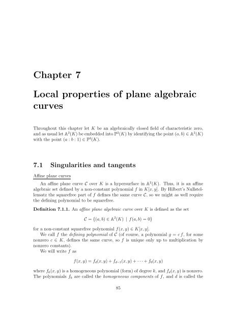
Example 7.1.1. Let the curve C be defined by the equation<br />
f(x, y) = 0, P = (a, b) a simple point on C. Consider<br />
the line L through P (with slope µ/λ) defined by µx−λy =<br />
µa − λb, or parametrically by x = a + λt, y = b + µt. We<br />
get the points <strong>of</strong> intersection <strong>of</strong> C and L as the solutions <strong>of</strong><br />
f(a + λt, b + µt) = 0.<br />
An expansion <strong>of</strong> this equation in a Taylor series around<br />
P yields (f(a, b) = 0):<br />
(f x λ + f y µ)t + 1 2! (f xxλ 2 + 2f x f y λµ + f yy µ 2 )t 2 + . . . = 0.<br />
We get “higher order” intersection at P if some <strong>of</strong> these terms vanish, i.e. if λ, µ are<br />
such that f x λ + f y µ = 0, . . . . The line which yields this higher order intersection is<br />
what we want to call the tangent to C at P.<br />
87
For analyzing a singular point P on a curve C we need to know its multiplicity but<br />
also the multiplicities <strong>of</strong> the tangents. If all the r tangents at the r-fold point P are<br />
different, then this singularity is <strong>of</strong> well-behaved type. For instance, when we trace the<br />
curve through P we can simply follow the tangent and then approximate back onto<br />
the curve. This is not possible any more when some <strong>of</strong> the tangents are the same.<br />
Definition 7.1.4. A singular point P <strong>of</strong> multiplicity r on an affine <strong>plane</strong> curve C is<br />
called ordinary iff the r tangents to C at P are distinct, and non-ordinary otherwise.<br />
non-ordinary. An ordinary double point is a node.<br />
Example 7.1.2. We consider the following <strong>curves</strong> in A 2 (C). Pictures <strong>of</strong> such <strong>curves</strong><br />
can be helpful, but we have to keep in mind that we can only plot the real components<br />
<strong>of</strong> such <strong>curves</strong>, i.e. the components in A 2 (R). Interesting phenomena, such as singular<br />
points etc., might not be visible in the real <strong>plane</strong>.<br />
A : a(x, y) = y−x 2 = 0 B : b(x, y) = y 2 −x 3 +x = 0 C : c(x, y) = y 2 −x 3<br />
D : d(x, y) = y 2 −x 3 −x 2 = 0 E : e(x, y) = (x 2 +y 2 ) 2 +3x 2 y−y 3 F : f(x, y) = (x 2 +y 2 ) 3 −4x 2 y 2<br />
The <strong>curves</strong> A, B are non-singular. The only singular point on C, D, E and F is the<br />
origin (0, 0).<br />
The linear forms in the equations for A and B define the tangents to these <strong>curves</strong><br />
at the origin.<br />
The forms <strong>of</strong> lowest degree in C, D, E and F are y 2 , y 2 −x 2 = (y −x)(y +x), 3x 2 y −<br />
y 3 = y( √ 3x − y)( √ 3x + y) and −4x 2 y 2 . The factors <strong>of</strong> these forms <strong>of</strong> lowest degree<br />
determine the tangents to these <strong>curves</strong> at the origin.<br />
Intersecting F by the line x = y we get the point P = ( √ 1 1<br />
2<br />
, √2 ).<br />
∂f<br />
∂x (P) = (6x5 + 12x 3 y 2 + 6xy 4 − 8xy 2 )(P) = √ 2,<br />
∂f<br />
∂y (P) = √ 2.<br />
88
So the tangent to F at P is defined by<br />
√<br />
2(x −<br />
1 √2 ) + √ 2(y − 1 √<br />
2<br />
) = 0 ∼ x + y − √ 2 = 0.<br />
D has a node at the origin. E has an ordinary 3–fold point at the origin. C and F both<br />
have a non–ordinary singular point at the origin.<br />
Lemma 7.1.1. Let C be an affine <strong>plane</strong> curve defined by the squarefree polynomial<br />
f = ∏ n<br />
i=1 f i where all the components f i are irreducible. Let P be a point in A 2 (K).<br />
Then the following holds:<br />
(1) mult P (C) = ∑ n<br />
i=1 mult P(C i ), where C i is the component <strong>of</strong> C defined by f i .<br />
(2) If L is a tangent to C i at P with multiplicity s i , then L is a tangent to C at P<br />
with multiplicity ∑ n<br />
i=1 s i.<br />
Pro<strong>of</strong>.<br />
(1) By the remark above we may assume that P is the origin. Let<br />
f i (x, y) =<br />
∑n i<br />
j=s i<br />
g i,j (x, y) for i = 1, . . .,n,<br />
where n i is the degree <strong>of</strong> C i , s i =mult P (C i ), and g i,j is the homogeneous component<br />
<strong>of</strong> f i <strong>of</strong> degree j. Then the lowest degree homogeneous component <strong>of</strong> f is ∏ n<br />
i=1 g i,s i<br />
.<br />
Hence, (1) follows from Remark (3).<br />
(2) follows directly from Remark (4) and from the expression <strong>of</strong> the lowest degree<br />
homogeneous component <strong>of</strong> f deduced in the pro<strong>of</strong> <strong>of</strong> statement (1).<br />
Example 7.1.3. Determine the singular points and the tangents at these singular<br />
points to the following <strong>curves</strong>:<br />
(a) f 1 = y 3 − y 2 + x 3 − x 2 + 3y 2 x + 3x 2 y + 2xy,<br />
(b) f 2 = x 4 + y 4 − x 2 y 2 ,<br />
(c) f 3 = x 3 + y 3 − 3x 2 − 3y 2 + 3xy + 1,<br />
(d) f 4 = y 2 + (x 2 − 5)(4x 4 − 20x 2 + 25).<br />
Plot the real components (i.e. in A 2 (R)) <strong>of</strong> these <strong>curves</strong>.<br />
Theorem 7.1.2. An affine <strong>plane</strong> curve has only finitely many singular points.<br />
Pro<strong>of</strong>: Let C be an affine <strong>plane</strong> curve with defining polynomial f, let f = f 1 · · ·f r<br />
be the irreducible factorization <strong>of</strong> f, and let C i be the component generated by f i<br />
(note that f is squarefree, so the f i ’s are pairwise relatively prime). Then, applying<br />
89
Lemma 7.1.1. one deduces that the singular points <strong>of</strong> C are the singular points <strong>of</strong> each<br />
component C i and the intersection points <strong>of</strong> all pairs <strong>of</strong> components (i.e. the points in<br />
the affine <strong>algebraic</strong> sets V (f i , f j ), i ≠ j). Hence the set W <strong>of</strong> singular points <strong>of</strong> C is:<br />
W = V<br />
(<br />
f, ∂f<br />
∂x , ∂f )<br />
=<br />
∂y<br />
r⋃<br />
V<br />
i=1<br />
(<br />
f i , ∂f i<br />
∂x , ∂f )<br />
i<br />
∪ ⋃ V (f i , f j ).<br />
∂y<br />
i≠j<br />
Now, observe that gcd(f i , f j ) = 1 for i ≠ j. Thus, applying Theorem 3.3.5., we get that,<br />
for i ≠ j, V (f i , f j ) is finite. Similarly, since f i is irreducible and deg( ∂f i<br />
), ∂x deg(∂f i<br />
) < ∂y<br />
deg(f), one deduces that gcd(f i , ∂f i<br />
, ∂f i) = 1. Therefore, again by Theorem 3.3.5, we<br />
∂x ∂y<br />
conclude that W is finite.<br />
Projective <strong>plane</strong> <strong>curves</strong><br />
A projective <strong>plane</strong> curve is a hypersurface in the projective <strong>plane</strong>.<br />
Definition 7.1.5. A projective <strong>plane</strong> <strong>algebraic</strong> curve over K is defined as the set<br />
C = {(a : b : c) ∈ P 2 (K) | F(a, b, c) = 0}<br />
for a non-constant squarefree homogeneous polynomial F(x, y, z) ∈ K[x, y, z].<br />
We call F the defining polynomial <strong>of</strong> C (<strong>of</strong> course, a polynomial G = c F, for some<br />
nonzero c ∈ K defines the same curve, so F is unique only up to multiplication by<br />
nonzero constants).<br />
Similarly as in Definition 7.1.1. the concepts <strong>of</strong> degree, components and irreducibility<br />
are introduced.<br />
Also, as in the case <strong>of</strong> affine <strong>curves</strong>, we will sometimes need to refer to multiple<br />
components <strong>of</strong> a projective <strong>plane</strong> curve. Again, one introduces this notion by extending<br />
the concept <strong>of</strong> curve to arbitrary forms. We will also always explicitly indicate when<br />
we make use <strong>of</strong> this generalization.<br />
As we saw in <strong>Chapter</strong> 5, there is a close relationship between affine and projective<br />
<strong>algebraic</strong> sets. Thus, associated to every affine curve there is a projective curve (its<br />
projective closure).<br />
Definition 7.1.6. The projective <strong>plane</strong> curve C ∗ corresponding to an affine <strong>plane</strong> curve<br />
C over K is the projective closure <strong>of</strong> C in P 2 (K).<br />
If the affine curve C is defined by the polynomial f(x, y), then from Section 5.2 we<br />
immediately get that the corresponding projective curve C ∗ is defined by the homogenization<br />
F(x, y, z) <strong>of</strong> f(x, y). Therefore, if f(x, y) = f d (x, y)+f d−1 (x, y)+· · ·+f 0 (x, y)<br />
is the decomposition <strong>of</strong> f into forms, then F(x, y, z) = f d (x, y) + f d−1 (x, y)z + · · · +<br />
f 0 (x, y)z d , and<br />
C ∗ = {(a : b : c) ∈ P 2 (K) | F(a, b, c) = 0}.<br />
90
Every point (a, b) on C corresponds to a point on (a : b : 1) on C ∗ , and every additional<br />
point on C ∗ is a point at infinity. In other words, the first two coordinates <strong>of</strong> the<br />
additional points are the nontrivial solutions <strong>of</strong> f d (x, y). Thus, the curve C ∗ has only<br />
finitely many points at infinity. Of course, a projective curve, not associated to an<br />
affine curve, could have z = 0 as a component and therefore have infinitely many<br />
points at infinity.<br />
On the other hand, associated to every projective curve there are infinitely many<br />
affine <strong>curves</strong>. We may take any line in P 2 (K) as the line at infinity, by a linear change<br />
<strong>of</strong> coordinates move it to z = 0, and then dehomogenize. But in practice we mostly<br />
use dehomogenizations provided by taking the axes as lines at infinity. More precisely,<br />
if C is the projective curve defined by the form F(x, y, z), we denote by C ∗,z the affine<br />
<strong>plane</strong> curve defined by F(x, y, 1). Similarly, we consider C ∗,y , and C ∗,x .<br />
So, any point P on a projective curve C corresponds to a point on a suitable affine<br />
version <strong>of</strong> C. The notions <strong>of</strong> multiplicity <strong>of</strong> a point and tangents at a point are local<br />
<strong>properties</strong>. So for determining the multiplicity <strong>of</strong> P at C and the tangents to C at<br />
P we choose a suitable affine <strong>plane</strong> (by dehomogenizing w.r.t to one <strong>of</strong> the projective<br />
variables) containing P, determine the multiplicity and tangents there, and afterwards<br />
homogenize the tangents to move them back to the projective <strong>plane</strong>. This process does<br />
not depend on the particular dehomogenizing variable (compare, for instance, [Ful69]<br />
Chap. 5).<br />
Theorem 7.1.3. P ∈ P 2 (K) is a singularity <strong>of</strong> the projective <strong>plane</strong> curve C defined<br />
by the homogeneous polynomial F(x, y, z) if and only if ∂F ∂F ∂F<br />
(P) = (P) = (P) = 0.<br />
∂x ∂y ∂z<br />
Pro<strong>of</strong>. Let d = deg(F). We may assume w.l.o.g. that P is not on the line at infinity<br />
z = 0, i.e. P = (a : b : 1). Let C ∗,z be the affine curve defined by f(x, y) = F(x, y, 1)<br />
and let P ∗ = (a, b) be the image <strong>of</strong> P in this affine version <strong>of</strong> the <strong>plane</strong>.<br />
P is a singular point <strong>of</strong> C if and only if P ∗ is a singular point <strong>of</strong> C ∗,z , i.e. if and only<br />
if<br />
f(P ∗ ) = ∂f<br />
∂x (P ∗) = ∂f<br />
∂y (P ∗) = 0.<br />
But<br />
∂f<br />
∂x (P ∗) = ∂F<br />
∂x (P),<br />
∂f<br />
∂y (P ∗) = ∂F<br />
∂y (P).<br />
Furthermore, by Euler’s Formula for homogeneous polynomials 1 we have<br />
The theorem now follows at once.<br />
x · ∂F ∂F ∂F<br />
(P) + y · (P) + z · (P) = d · F(P).<br />
∂x ∂y ∂z<br />
1 Euler’s formula for homogeneous polynomials F(x 1 , x 2 , x 3 ):<br />
deg(F)<br />
∑ 3<br />
i=1 x i · ∂F<br />
∂x i<br />
= n · F, where n =<br />
91
By an inductive argument this theorem can be extended to higher multiplicities.<br />
We leave the pro<strong>of</strong> as an exercise.<br />
Theorem 7.1.4. P ∈ P 2 (K) is a point <strong>of</strong> multiplicity at least r on the projective<br />
<strong>plane</strong> curve C defined by the homogeneous polynomial F(x, y, z) <strong>of</strong> degree d (where<br />
r ≤ d) if and only if all the (r − 1)-th partial derivatives <strong>of</strong> F vanish at P.<br />
We finish this section with an example where all these notions are illustrated.<br />
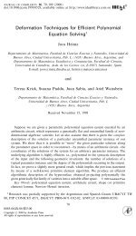
Example 7.1.4. Let C be the projective <strong>plane</strong> curve over C defined by the homogeneous<br />
polynomial:<br />
F(x, y, z) = −4 y 4 z 3 x 2 + 2 y 7 x 2 + y 9 + 3 y 7 z 2 − 9 y 6 x 2 z − 2 x 8 z + 2 x 8 y + 3 x 4 y 5<br />
−y 6 z 3 + 4 x 6 y 3 − 7 x 6 y 2 z + 5 x 6 y z 2 + 10 x 2 y 5 z 2 − 11 x 4 y 4 z<br />
+9 x 4 y 3 z 2 − 4 x 4 y 2 z 3 + y 3 z 4 x 2 − 3 y 8 z<br />
The degree <strong>of</strong> the curve is 9. In Figure 7.1. the real part <strong>of</strong> C ⋆,z is plotted.<br />
3<br />
y<br />
2<br />
1<br />
–3 –2 –1 0 1 x 2 3<br />
–1<br />
Figure 7.1: Real part <strong>of</strong> C ⋆,z<br />
First, we compute the finitely many points at infinity <strong>of</strong> the curve. We observe that<br />
F(x, y, 0) = y(2x 4 + y 4 )(y 2 + x 2 ) 2<br />
does not vanish identically, so the line z = 0 is not a component <strong>of</strong> C. In fact, the<br />
points at infinity are (1 : 0 : 0), (1 : α : 0) where α 4 + 2 = 0, and the cyclic points<br />
(1 : ±i : 0). Hence, the line at infinity intersects C at 7 points (compare to Bézout’s<br />
Theorem, in this chapter).<br />
92
Now, we proceed to determine and analyze the singularities. We apply Theorem<br />
7.1.3. Solving the system<br />
{ ∂F<br />
∂x<br />
= 0,<br />
∂F<br />
∂y<br />
= 0,<br />
∂F<br />
∂z = 0}<br />
we find that the singular points <strong>of</strong> C are<br />
(1 : ±i : 0), (0 : 0 : 1), (± 1<br />
3 √ 3 : 1 3 : 1), (±1 2 , 1 : 1), (0 : 1 : 1), and (±1 : α : 1)<br />
2<br />
where α 3 + α − 1 = 0. So C has 11 singular points.<br />
Now we compute the multiplicities and the tangents to C at each singular point. For<br />
this purpose, we determine the first non-vanishing term in the corresponding Taylor<br />
expansion. The result <strong>of</strong> this computation is shown in Table 7.1. In this table we<br />
denote the singularities <strong>of</strong> C as follows:<br />
P ± 1 := (1 : ±i : 0), P 2 := (0 : 0 : 1), P ± 3 := (± 1<br />
3 √ 3 : 1 3 : 1),<br />
P ± 4 := (±1 2 , 1 2 : 1), P 5 := (0 : 1 : 1), P ± α<br />
:= (±1 : α : 1)<br />
All these singular points are ordinary, except the affine origin (0 : 0 : 1). Factoring<br />
F over C we get<br />
F(x, y, z) = (x 2 + y 2 − yz)(y 3 + yz 2 − zx 2 )(y 4 − 2y 3 z + y 2 z 2 − 3yzx 2 + 2x 4 ).<br />
Therefore, C decomposes into a union <strong>of</strong> a conic, a cubic, and a quartic. Furthermore,<br />
(0 : 0 : 1) is a double point on the quartic, a double point on the cubic, and a simple<br />
point on the conic. Thus, applying Lemma 7.1.1, the multiplicity <strong>of</strong> C at (0 : 0 : 1) is<br />
5. (0 : 1 : 1) is a double point on the quartic and a simple point on the conic. Hence,<br />
the multiplicity <strong>of</strong> C at (0 : 1 : 1) is 3. (± 1 : 1 : 1) are simple points on the conic and<br />
2 2<br />
the cubic. (± 1<br />
3 √ : 1 : 1) are simple points on the quartic and the cubic. Similarly, the<br />
2 3<br />
points (±1 : α : 1) are also simple points on the quartic and the cubic (two <strong>of</strong> them<br />
are real, and four <strong>of</strong> them complex). Finally, the cyclic points are simple points on the<br />
cubic and the conic. Hence, all these singular points are double points on C.<br />
93
point tangents multiplicity<br />
P + 1 (2y − z − 2ix)(2y + z − 2ix) 2<br />
P − 1 (2y + z + 2ix)(2y − z + 2ix) 2<br />
P 2 y 3 x 2 5<br />
P + 3 (8x + √ 2z − 7 √ 2y)(28x − 5 √ 2z + √ 2y) 2<br />
P − 3 (8x − √ 2z + 7 √ 2y)(28x + 5 √ 2z − √ 2y) 2<br />
P + 4 (2x − z)(2x − 4y + z) 2<br />
P − 4 (2x + z)(2x + 4y − z) 2<br />
P 5 (y − z)(3x 2 + 2yz − y 2 − z 2 ) 3<br />
P + α ((1 + 1 2 α + 1 2 α2 )z + x + (− 5 2 − 1 2 α − 2α2 )y) 2<br />
((− 35<br />
146 − 23<br />
73 α + 1 73 α2 )z + x + (− 65<br />
146 − 1 73 α − 111<br />
146 α2 )y)<br />
P − α ((−1 − 1 2 α − 1 2 α2 )z + x + ( 5 2 + 1 2 α + 2α2 )y) 2<br />
(( 35<br />
146 + 23<br />
73 α − 1<br />
73 α2 )z + x + ( 65<br />
146 + 1<br />
73 α + 111<br />
146 α2 )y)<br />
Table 7.1.<br />
94
7.2 Intersection <strong>of</strong> Curves<br />
In this section we analyze the intersection <strong>of</strong> two <strong>plane</strong> <strong>curves</strong>. Since <strong>curves</strong> are <strong>algebraic</strong><br />
sets, and since the intersection <strong>of</strong> two <strong>algebraic</strong> sets is again an <strong>algebraic</strong> set, we<br />
see that the intersection <strong>of</strong> two <strong>plane</strong> <strong>curves</strong> is an <strong>algebraic</strong> set in the <strong>plane</strong> consisting<br />
<strong>of</strong> 0-dimensional and 1-dimensional components. The ground field K is <strong>algebraic</strong>ally<br />
closed, so the intersection <strong>of</strong> two <strong>curves</strong> is non-empty. In fact, the intersection <strong>of</strong> two<br />
<strong>curves</strong> contains a 1-dimensional component, i.e. a curve, if and only if the gcd <strong>of</strong> the<br />
corresponding defining polynomials is not constant, or equivalently if both <strong>curves</strong> have<br />
a common component. Hence, in this case the intersection is given by the gcd.<br />
Therefore, the problem <strong>of</strong> analyzing the intersection <strong>of</strong> <strong>curves</strong> is reduced to the case<br />
<strong>of</strong> two <strong>curves</strong> without common components. There are two questions which we need<br />
to answer. First, we want to compute the finitely many intersection points <strong>of</strong> the two<br />
<strong>curves</strong>. This means solving a zero dimensional system <strong>of</strong> two bivariate polynomials.<br />
Second, we also want to analyze the number <strong>of</strong> intersection points <strong>of</strong> the <strong>curves</strong> when<br />
the two <strong>curves</strong> do not have common components. This counting <strong>of</strong> intersections points<br />
with proper multiplicities is achieved by Bézout’s Theorem (in this section). For this<br />
purpose, one introduces the notion <strong>of</strong> multiplicity <strong>of</strong> intersection.<br />
We start with the problem <strong>of</strong> computing the intersection points. Let C and D be<br />
two projective <strong>plane</strong> <strong>curves</strong> defined by F(x, y, z) and G(x, y, z), respectively, such that<br />
gcd(F, G) = 1. We want to compute the finitely many points in V (F, G). Since we<br />
are working in the <strong>plane</strong>, the solutions <strong>of</strong> this system <strong>of</strong> <strong>algebraic</strong> equations can be<br />
determined by resultants.<br />
First, we observe that if both polynomials F and G are bivariate forms in the same<br />
variables, say F, G ∈ K[x, y] (similarly if F, G ∈ K[x, z] or F, G ∈ K[y, z]), then each<br />
curve is a finite union <strong>of</strong> lines passing through (0 : 0 : 1). Hence, since the <strong>curves</strong> do<br />
not have common components, one has that C and D intersect only in (0 : 0 : 1).<br />
So now let us assume that at least one <strong>of</strong> the defining polynomials is not a bivariate<br />
form in x and y, say F ∉ K[x, y]. Then, we consider the resultant R(x, y) <strong>of</strong> F and<br />
G with respect to z. Since C and D do not have common components, R(x, y) is not<br />
identically zero. Furthermore, since deg z (F) ≥ 1 and G is not constant, the resultant<br />
R is a non-constant bivariate homogeneous polynomial. Hence it factors as<br />
r∏<br />
R(x, y) = (b i x − a i y) n i<br />
i=1<br />
for some a i , b i ∈ K, and r i ∈ N. For every (a, b) ∈ K 2 such that R(a, b) = 0 there exists<br />
c ∈ K such that F(a, b, c) = G(a, b, c) = 0, and conversely. Therefore, the solutions<br />
<strong>of</strong> R provide the intersection points. Since (0 : 0 : 0) is not a point in P 2 (K), but<br />
it might be the formal result <strong>of</strong> extending the solution (0, 0) <strong>of</strong> R, we check whether<br />
(0 : 0 : 1) is an intersection point. The remaining intersection points are given by<br />
(a i : b i : c i,j ), where a i , b i are not simultaneously zero, and c i,j are the roots in K <strong>of</strong><br />
gcd(F(a i , b i , z), G(a i , b i , z)).<br />
95
Example 7.2.1. Let C and D be the projective <strong>plane</strong> <strong>curves</strong> defined by F(x, y, z) =<br />
x 2 + y 2 − yz and G(x, y, z) = y 3 + x 2 y − x 2 z, respectively. Observe that these <strong>curves</strong><br />
are the conic and cubic that appear in Example 7.1.4. Since gcd(F, G) = 1, C and D<br />
do not have common components. Obviously (0 : 0 : 1) is an intersection point. For<br />
determining the other intersection points, we compute<br />
R(x, y) = res z (F, G) = x 4 − y 4 = (x − y)(x + y)(x 2 + y 2 ).<br />
For extending the solutions <strong>of</strong> R to the third coordinate we compute<br />
gcd(F(1, 1, z), G(1, 1, z)) = z − 2, gcd(F(1, −1, z), G(1, −1, z)) = z + 2,<br />
gcd(F(1, ±i, z), G(1, ±i, z)) = z. So the intersection points <strong>of</strong> C and D are<br />
(0 : 0 : 1), ( 1 2 : 1 2 : 1), (1 2 : −1 2<br />
: 1), (1 : i : 0), (1 : −i : 0)<br />
We now proceed to the problem <strong>of</strong> analyzing the number <strong>of</strong> intersections <strong>of</strong> two<br />
projective <strong>curves</strong> without common components. For this purpose, we first study upper<br />
bounds, and then we see how these upper bounds can always be reached by a suitable<br />
definition <strong>of</strong> the notion <strong>of</strong> intersection multiplicity.<br />
Theorem 7.2.1. Let C and D be two projective <strong>plane</strong> <strong>curves</strong> without common components<br />
and degrees n and m, respectively. Then the number <strong>of</strong> intersection points <strong>of</strong><br />
C and D is at most n · m.<br />
Pro<strong>of</strong>: First observe that the number <strong>of</strong> intersection points is invariant under linear<br />
changes <strong>of</strong> coordinates. Let k be the number <strong>of</strong> intersection points <strong>of</strong> C and D. W.l.o.g<br />
we assume that (perhaps after a suitable linear change <strong>of</strong> coordinates) P = (0 : 0 : 1)<br />
is not a point on C or D and also not on a line connecting any pair <strong>of</strong> intersection<br />
points <strong>of</strong> C and D. Let F(x, y, z) and G(x, y, z) be the defining polynomials <strong>of</strong> C and<br />
D, respectively. Note that since (0 : 0 : 1) is not on the <strong>curves</strong>, we have<br />
F(x, y, z) = A 0 z n + A 1 z n−1 + · · · + A n ,<br />
G(x, y, z) = B 0 z m + B 1 z m−1 + · · · + B m ,<br />
where A 0 , B 0 are non-zero constants and A i , B j are homogeneous polynomials <strong>of</strong> degree<br />
i, j, respectively. Let R(x, y) be the resultant <strong>of</strong> F and G with respect to z. Since the<br />
<strong>curves</strong> do not have common components, R is a non-zero homogeneous polynomial in<br />
K[x, y] <strong>of</strong> degree n ·m (compare [Wal50], Theorem I.10.9 on p.30). Furthermore, as we<br />
have already seen, each linear factor <strong>of</strong> R generates a set <strong>of</strong> intersection points. Thus,<br />
if we can prove that each linear factor generates exactly one intersection point, we have<br />
shown that k ≤deg(R) = n · m. Let us assume that l(x, y) = bx − ay is a linear factor<br />
<strong>of</strong> R. l(x, y) generates the solution (a, b) <strong>of</strong> R, which by Theorem 4.3.3 in [Win96] can<br />
be extended to a common solution <strong>of</strong> F and G. So now let us assume that the partial<br />
solution (a, b) can be extended to at least two different intersection points P 1 and P 2<br />
96
<strong>of</strong> C and D. But this implies that the line bx −ay passes through P 1 , P 2 and (0 : 0 : 1),<br />
which we have excluded.<br />
Given two projective <strong>curves</strong> <strong>of</strong> degrees n and m, respectively, and without common<br />
components, one gets exactly n · m intersection points if the intersection points are<br />
counted properly. This leads to the definition <strong>of</strong> multiplicity <strong>of</strong> intersection. First<br />
we present the notion for <strong>curves</strong> such that the point (0 : 0 : 1) is not on any <strong>of</strong> the<br />
two <strong>curves</strong>, nor on any line connecting two <strong>of</strong> their intersection points. Afterwards,<br />
we observe that the concept can be extended to the general case by means <strong>of</strong> linear<br />
changes <strong>of</strong> coordinates.<br />
Definition 7.2.1. Let C and D be projective <strong>plane</strong> <strong>curves</strong>, without common components,<br />
such that (0 : 0 : 1) is not on C or D and such that it is not on any line<br />
connecting two intersection points <strong>of</strong> C and D. Let P = (a : b : c) ∈ C ∩ D, and let<br />
F(x, y, z) and G(x, y, z) be the defining polynomials <strong>of</strong> C and D, respectively. Then,<br />
the multiplicity <strong>of</strong> intersection <strong>of</strong> C and D at P (we denote it by mult P (C, D)) is defined<br />
as the multiplicity <strong>of</strong> the factor bx − ay in the resultant <strong>of</strong> F and G with respect to z.<br />
If P ∉ C ∩ D then we define the multiplicity <strong>of</strong> intersection at P as 0.<br />
We observe that the condition on (0 : 0 : 1), required in Definition 7.2.1, can<br />
be avoided by means <strong>of</strong> linear changes <strong>of</strong> coordinates. Moreover, the extension <strong>of</strong><br />
the definition to the general case does not depend on the particular linear change <strong>of</strong><br />
coordinates, as remarked in [Wal50], Sect. IV.5. Indeed, since C and D do not have<br />
common components the number <strong>of</strong> intersection points is finite. Therefore, there always<br />
exist linear changes <strong>of</strong> coordinates satisfying the required conditions in the definition.<br />
Furthermore, as we have remarked in the last part <strong>of</strong> the pro<strong>of</strong> <strong>of</strong> Theorem 7.2.1., if<br />
T is any linear change <strong>of</strong> coordinates satisfying the conditions <strong>of</strong> the definition, each<br />
factor <strong>of</strong> the corresponding resultant is generated by exactly one intersection point.<br />
Therefore, the multiplicity <strong>of</strong> the factors in the resultant is preserved by this type <strong>of</strong><br />
linear changes <strong>of</strong> coordinates.<br />
Theorem 7.2.2. (Bézout’s Theorem) Let C and D be two projective <strong>plane</strong> <strong>curves</strong><br />
without common components and degrees n and m, respectively. Then<br />
n · m = ∑<br />
mult P (C, D).<br />
P ∈C∩D<br />
Pro<strong>of</strong>: Let us assume w.l.o.g. that C and D are such that (0 : 0 : 1) is not on C<br />
or D nor on any line connecting two <strong>of</strong> their intersection points. Let F(x, y, z) and<br />
G(x, y, z) be the defining polynomials <strong>of</strong> C and D, respectively. Then the resultant<br />
R(x, y) <strong>of</strong> F and G with respect to z is a non-constant homogeneous polynomial <strong>of</strong><br />
degree n·m (compare the pro<strong>of</strong> <strong>of</strong> Theorem 7.2.1). Furthermore, if {(a i : b i : c i )} i=1,...,r<br />
are the intersection points <strong>of</strong> C and D (note that (0 : 0 : 1) is not one <strong>of</strong> them) then<br />
97
we get<br />
R(x, y) =<br />
r∏<br />
(b i x − a i y) n i<br />
,<br />
i=1<br />
where n i is, by definition, the multiplicity <strong>of</strong> intersection <strong>of</strong> C and D at (a i : b i : c i ).<br />
Therefore, the formula holds.<br />
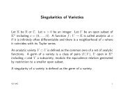
Example 7.2.2. We consider the two cubics C and D <strong>of</strong> Figure 7.2 defined by the<br />
polynomials<br />
F(x, y, z) = 516<br />
85 z3 − 352<br />
85 yz2 − 7 17 y2 z+ 41<br />
85 y3 + 172<br />
85 xz2 − 88<br />
85 xyz+ 1 85 y2 x−3x 2 z+x 2 y−x 3 ,<br />
G(x, y, z) = −132z 3 +128yz 2 −29y 2 z−y 3 +28xz 2 −76xyz+31y 2 x+75x 2 z−41x 2 y+17x 3 ,<br />
respectively.<br />
4<br />
y<br />
2<br />
4<br />
y<br />
2<br />
–4 –2 0 2 x 4<br />
–2<br />
–4 –2 0 2 x 4<br />
–2<br />
–4<br />
–4<br />
Figure 7.2: Real part <strong>of</strong> C ⋆,z (Left), Real part <strong>of</strong> D ⋆,z (Right)<br />
Let us determine the intersection points <strong>of</strong> these two cubics and their corresponding<br />
multiplicities <strong>of</strong> intersection. For this purpose, we first compute the resultant<br />
R(x, y) = res z (F, G) = − 5474304 x 4 y (3x + y) (x + 2y) (x + y) (x − y).<br />
25<br />
For each factor (ax − by) <strong>of</strong> the resultant R(x, y) we obtain the polynomial D(z) =<br />
gcd(F(a, b, z), G(a, b, z)) in order to find the intersection points generated by this factor.<br />
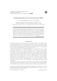
The next table shows the results <strong>of</strong> this computation (compare to Figure 7.3.):<br />
98
factor D(z) intersection point multipl. <strong>of</strong> intersection<br />
x 4 (2z − 1) 2 P 1 = (0 : 2 : 1) 4<br />
y z + 1/3 P 2 = (−3 : 0 : 1) 1<br />
3x + y z − 1 P 3 = (1 : −3 : 1) 1<br />
x + 2y z + 1 P 4 = (−2 : 1 : 1) 1<br />
x + y z + 1 P 5 = (−1 : 1 : 1) 1<br />
x − y z − 1 P 6 = (1 : 1 : 1) 1<br />
Table 7.2.<br />
4<br />
y<br />
2<br />
–4 –2 0 2 x 4<br />
–2<br />
–4<br />
Figure 7.3: Joint picture <strong>of</strong> the real parts <strong>of</strong> C ⋆,z and D ⋆,z<br />
Furthermore, since (0 : 0 : 1) is not on the cubics nor on any line connecting their<br />
intersection points, the multiplicity <strong>of</strong> intersection is 4 for P 1 , and 1 for the other<br />
points. It is also interesting to observe that P 1 is a double point on each cubic (compare<br />
Theorem 7.2.3. (5)).<br />
Some authors introduce the notion <strong>of</strong> multiplicity <strong>of</strong> intersection axiomatically (see,<br />
for instance, [Ful69], Sect. 3.3). The following theorem shows that these axioms are<br />
satified for our definition.<br />
Theorem 7.2.3. Let C and D be two projective <strong>plane</strong> <strong>curves</strong>, without common components,<br />
defined by the polynomials F and G, respectively, and let P ∈ P 2 (K). Then<br />
the following holds:<br />
(1) mult P (C, D) ∈ N.<br />
(2) mult P (C, D) = 0 if and only if P ∉ C ∩ D. Furthermore, mult P (C, D) depends<br />
only on those components <strong>of</strong> C and D containing P.<br />
99
(3) If T is a linear change <strong>of</strong> coordinates, and C ′ , D ′ , P ′ are the imagines <strong>of</strong> C, D,<br />
and P under T, respectively, then mult P (C, D) = mult P ′(C ′ , D ′ ).<br />
(4) mult P (C, D) = mult P (D, C).<br />
(5) mult P (C, D) ≥ mult P (C) · mult P (D). Furthermore, equality holds if and only C<br />
and D intersect transversally at P (i.e. if the <strong>curves</strong> have no common tangents<br />
at P).<br />
(6) Let C 1 , . . .,C r and D 1 , . . .,D s be the irreducible components <strong>of</strong> C and D respectively.<br />
Then<br />
r∑ s∑<br />
mult P (C, D) = mult P (C i , D j ).<br />
i=1<br />
(7) mult P (C, D) = mult P (C, D H ), where D H is the curve defined by G + HF for an<br />
arbitrary form H ∈ K[x, y, z] (i.e. the intersection multiplicity does not depend<br />
on the particular representative G in the coordinate ring <strong>of</strong> C).<br />
Pro<strong>of</strong>: We have already remarked above that the intersection multiplicity is independent<br />
<strong>of</strong> a particular linear change <strong>of</strong> coordinates. Statements (1),(2),and (4) can be<br />
easily deduced from the definition <strong>of</strong> multiplicity <strong>of</strong> intersection, and we leave them to<br />
the reader.<br />
A pro<strong>of</strong> <strong>of</strong> (5) can be found for instance in [Wal50], Chap. IV.5, Theorem 5.10.<br />
(6) Let us assume without loss <strong>of</strong> generality that C and D satisfy the requirements <strong>of</strong><br />
Definition 7.2.1. That is, (0 : 0 : 1) is not on the <strong>curves</strong> nor on any line connecting<br />
their intersection points. Let F i , i = 1, . . ., r, and G j , j = 1 . . .,s, be the defining polynomials<br />
<strong>of</strong> C i and D j , respectively. Then we use the following fact: if A, B, C ∈ D[x],<br />
where D is an integral domain, then res x (A, B · C) = res x (A, B) · res x (A, C) (see, for<br />
instance, [BCL83] Theorem 3 p. 178). Hence, (6) follows immediately from<br />
j=1<br />
r∏ s∏<br />
res z ( F i , G j ) =<br />
i=1 j=1<br />
r∏ s∏<br />
res z (F i , G j ) =<br />
i=1 j=1<br />
r∏ s∏<br />
res z (F i , G j ).<br />
i=1 j=1<br />
(7) Let H ∈ K[x, y, z] be a form. Obviously P ∈ C ∩ D if and only if P ∈ C ∩<br />
D H . We assume without loss <strong>of</strong> generality that C and D satisfy the conditions <strong>of</strong> the<br />
Definition 7.2.1, and also C and D H satisfy these conditions. Then, mult P (C, D) and<br />
mult P (C, D H ) are given by the multiplicities <strong>of</strong> the corresponding factors in res z (F, G)<br />
and res z (F, G + H F), respectively. Now, we use the following property <strong>of</strong> resultants:<br />
if A, B, C ∈ D[x], where D is an integral domain, and a is the leading coefficient <strong>of</strong><br />
A, then res x (A, B) = a deg x (B)−deg x (A C+B) res x (A, A C + B) (see, for instance, [BCL83]<br />
Theorem 4, p. 178). (7) follows directly from this fact, since the leading coefficient <strong>of</strong><br />
F in z is a non-zero constant (note that (0 : 0 : 1) is not on C).<br />
100
From Theorem 7.2.3 one can extract an alternative algorithm for computing the<br />
intersection multiplicity:<br />
Because <strong>of</strong> (3) we may assume that P = (0, 0).<br />
Since the intersection multiplicity is a local property, we may work in the affine<br />
<strong>plane</strong>. Consider the <strong>curves</strong> defined by f(x, y) and g(x, y). We check whether P lies<br />
on a common component <strong>of</strong> f and g, i.e. whether gcd(f, g)(P) = 0. If this is the<br />
case we set mult P (f ∩ g) = ∞, because <strong>of</strong> (1). Otherwise we continue to determine<br />
mult P (f ∩ g) ∈ N 0 .<br />
We proceed inductively. The base case mult P (f ∩ g) = 0 is covered by (2). Our<br />
induction hypothesis is<br />
mult P (a ∩ b) can be determined for mult P (a ∩ b) < n.<br />
So now let mult P (f ∩ g) = n > 0.<br />
Let f(x, 0), g(x, 0) ∈ K[x] be <strong>of</strong> degrees r, s, respectively. Because <strong>of</strong> (4) we can<br />
assume that r ≤ s.<br />
Case 1, r = −1: I.e. f(x, 0) = 0. In this case f = y · h for some h ∈ K[x, y], and<br />
because <strong>of</strong> (6)<br />
mult P (f ∩ g) = mult P (y ∩ g) + mult P (h ∩ g).<br />
Let m be such that g(x, 0) = x m (a 0 + a 1 x + . . .), a 0 ≠ 0. Note that g(x, 0) = 0 is<br />
impossible, since otherwise f and g would have the common component y, which we<br />
have excluded.<br />
mult P (y ∩ g) = (7) mult P (y ∩ g(x, 0)) = (2) mult P (y ∩ x m ) = (6) m · mult P (y ∩ x) = (5) m.<br />
Since P ∈ g, we have m > 0, so mult P (h ∩ g) < n. By the induction hypothesis, this<br />
implies that mult P (h ∩ g) can be determined.<br />
Case 2, r > −1: We assume that f(x, 0), g(x, 0) are monic. Otherwise we multiply f<br />
and g by suitable constants to make them monic. Let<br />
Because <strong>of</strong> (7) we have<br />
h = g − x s−r · f.<br />
mult P (f ∩ g) = mult P (f ∩ h) and deg(h(x, 0)) = t < s.<br />
Continuing this process (we might have to interchange f and h, if t < r) eventually,<br />
after finitely many steps, we reach a pair <strong>of</strong> <strong>curves</strong> a, b which can be handled by Case<br />
1.<br />
From these considerations we can immediately extract the following algorithm for<br />
computing intersection multiplicities.<br />
101
Algorithm INT MULT<br />
in: f, g ∈ K[x, y], P = (a, b) ∈ A 2 (K);<br />
out: M = mult P (f ∩ g);<br />
(1) if P ≠ (0, 0)<br />
then { P := (0, 0); f := f(x + a, y + b); g := g(x + a, y + b) };<br />
(2) if gcd(f, g)(P) = 0 then { M := ∞;return };<br />
(3) f 0 := f(x, 0); r := deg(f 0 );<br />
g 0 := g(x, 0); s := deg(g 0 );<br />
if r > s then interchange (f, f 0 , r) and (g, g 0 , s);<br />
while r > −1 do<br />
{ g := 1<br />
lc(g 0 ) · g − xs−r ·<br />
1<br />
lc(f 0 ) · f;<br />
g 0 := g(x, 0); s := deg(g 0 );<br />
if r > s then interchange (f, f 0 , r) and (g, g 0 , s) } ;<br />
(4) [r = −1]<br />
h := f/y; m := exponent <strong>of</strong> lowest term in g 0 ;<br />
M := m + INT MULT(h, g, P)<br />
Example 7.2.3. We determine the intersection multiplicity at the origin O = (0, 0)<br />
<strong>of</strong> the affine <strong>curves</strong> E, F defined by<br />
E : e(x, y) = (x 2 + y 2 ) 2 + 3x 2 y − y 3 , F : f(x, y) = (x 2 + y 2 ) 3 − 4x 2 y 2 .<br />
For ease <strong>of</strong> notation we don’t distinguish between the <strong>curves</strong> and their defining polynomials.<br />
We replace f by the following curve g:<br />
f(x, y) − (x 2 + y 2 )e(x, y) = y · ((x 2 + y 2 )(y 2 − 3x 2 ) − 4x 2 y) = y · g(x, y).<br />
Now we have<br />
We replace g by h:<br />
mult O (e ∩ f) = mult O (e ∩ y) + mult O (e ∩ g).<br />
g + 3e = y · (5x 2 − 3y 2 + 4y 3 + 4x 2 y) = y · h(x, y).<br />
So<br />
mult O (e ∩ f) = 2 · mult O (e ∩ y) + mult O (e ∩ h).<br />
102
mult O (e ∩ y) = (4),(7) mult O (x 4 ∩ y) = (6),(5) 4,<br />
mult O (e ∩ h) = (5) mult O (e) · mult O (h) = 6.<br />
Thus, mult O (E, F) = mult O (e ∩ f) = 14.<br />
Theorem 7.2.4. The line l is tangent to the curve f at the point P if and only if<br />
mult P (f ∩ l) > mult P (f).<br />
Pro<strong>of</strong>: By the property (5), l is tangent to f at P if and only if mult P (f ∩ l) ><br />
mult P (f) · mult P (l) = mult P (f).<br />
Theorem 7.2.5. If the line l is not a component <strong>of</strong> the curve f, then<br />
∑<br />
P ∈A 2 mult P (f ∩ l) ≤ deg(f).<br />
Pro<strong>of</strong>: Only points in f ∩ l can contribute to the sum. Let l be parametrized as<br />
{x = a + tb, y = c + td}. Let<br />
g(t) = f(a + tb, c + td) = α ·<br />
r∏<br />
(t − λ i ) e i<br />
,<br />
for α, e i ∈ K. g ≠ 0, since l is not a component <strong>of</strong> f.<br />
P ∈ f ∩ l if and only if P = P i = (a + λ i b, c + λ i d) for some 1 ≤ i ≤ r.<br />
If all the partial derivatives <strong>of</strong> f <strong>of</strong> order n vanish at P i , then by the chain rule also<br />
∂ n g<br />
∂t n (λ i) =<br />
So mult Pi (f) ≤ e i .<br />
Summarizing we get<br />
i=0<br />
i=1<br />
n∑<br />
( ) n ∂ n f<br />
i ∂x i ∂y n−1(a + λ ib, c + λ i d) · b i · d n−i = 0.<br />
∑<br />
P ∈A 2 mult P (f∩l) =<br />
r∑<br />
mult Pi (f∩l) = (5)<br />
i=1<br />
r∑<br />
i=1<br />
mult Pi (f)·mult Pi (l)<br />
} {{ }<br />
=1<br />
≤<br />
r∑<br />
e i ≤ deg(f).<br />
i=1<br />
103
7.3 Linear Systems <strong>of</strong> Curves<br />
Throughout this section we take into account the multiplities <strong>of</strong> components in <strong>algebraic</strong><br />
<strong>curves</strong>, i.e. the equations x 2 y = 0 and xy 2 = 0 determine two different <strong>curves</strong>.<br />
As always, we assume that the underlying field K is <strong>algebraic</strong>ally closed.<br />
A projective curve C <strong>of</strong> degree n is defined by a polynomial equation <strong>of</strong> the form<br />
∑<br />
a ijk x i y j z k = 0.<br />
i+j+k=n<br />
The number <strong>of</strong> coefficients a ijk in this homogeneous equation is (n + 1)(n + 2)/2 2 .<br />
The curve C is defined uniquely by these coefficients, and conversely the coefficients are<br />
determined uniquely by the curve C, up to a constant factor. Therefore, the coefficients<br />
can be regarded as projective coordinates <strong>of</strong> the curve C, and the set S n <strong>of</strong> projective<br />
<strong>curves</strong> <strong>of</strong> degree n can be regarded as points in a projective space P N , where<br />
N = (# <strong>of</strong> coeff.) − 1 = n(n + 3)/2.<br />
Definition 7.3.1. The <strong>curves</strong>, which constitute an r–dimensional subspace P r <strong>of</strong><br />
S n = P N , form a linear system <strong>of</strong> <strong>curves</strong> <strong>of</strong> dimension r. Such a system S is determined<br />
by r +1 independent <strong>curves</strong> F 0 , F 1 , . . .,F r in the system. The defining equation <strong>of</strong> any<br />
curve in S can be written in the form<br />
r∑<br />
λ i F i (x, y, z) = 0.<br />
i=0<br />
Since P r is also determined by N −r hyper<strong>plane</strong>s containing P r , the linear systems<br />
S can also be written as the intersection <strong>of</strong> these N − r hyper<strong>plane</strong>s. The equation <strong>of</strong><br />
such a hyper<strong>plane</strong> in P N is called a linear condition on the <strong>curves</strong> in S n , and a curve<br />
satisfies the linear condition iff it is a point in the hyper<strong>plane</strong>.<br />
Since N hyper<strong>plane</strong>s always have at least one point in common, we can always find<br />
a curve satisfying N or fewer linear conditions. In general, in an r–dimensional linear<br />
system <strong>of</strong> <strong>curves</strong> we can always find a curve satisfying r or fewer (additional) linear<br />
conditions.<br />
Example 7.3.1. We consider the system S 2 <strong>of</strong> quadratic <strong>curves</strong> (conics) over C. In<br />
S 2 we choose two <strong>curves</strong>, a circle F 0 and a parabola F 1 :<br />
F 0 (x, y, z) = x 2 + y 2 − z 2 , F 1 (x, y, z) = yz − x 2 .<br />
2 f(x, y) = a 0 (x)y n + a 1 (x)y n−1 + · · · + a n (x); so the number <strong>of</strong> terms is 1 + 2 + · · · + (n + 1) =<br />
(n + 1)(n + 2)/2<br />
104
F 0 and F 1 determine a 1–dimensional linear subsystem <strong>of</strong> S 2 . The defining equation <strong>of</strong><br />
a general curve in this subsystem is <strong>of</strong> the form<br />
or<br />
λ 0 F 0 + λ 1 F 1 = 0,<br />
(λ 0 − λ 1 )x 2 + λ 0 y 2 − λ 0 z 2 + λ 1 yz = 0.<br />
We get a linear condition by requiring that the point (1 : 2 : 1) should be a point on<br />
any curve. This forces λ 1 = −4λ 0 . The following curve (λ 0 = 1, λ 1 = −4) satisfies the<br />
condition:<br />
5x 2 + y 2 − z 2 − 4yz = 0.<br />
It is very common for linear conditions to arise from requirements such as “all<br />
<strong>curves</strong> in the subsystem should contain the point P as a point <strong>of</strong> multiplicity at least<br />
r, r ≥ 1.” This means that all the partial derivatives <strong>of</strong> order < r <strong>of</strong> the defining<br />
equation have to vanish at P. There are exactly r(r + 1)/2 such derivations, and they<br />
are homegeneous linear polynomials in the coefficients a ijk . Thus, such a requirement<br />
induces r(r + 1)/2 linear conditions on the <strong>curves</strong> <strong>of</strong> the subsystem.<br />
Definition 7.3.2. A point P <strong>of</strong> multiplicity ≥ r on all the <strong>curves</strong> in a linear system is<br />
called a base point <strong>of</strong> multiplicity r <strong>of</strong> the system. In particular, the linear subsystem <strong>of</strong><br />
S n which has the different points P 1 , . . .,P m as base points <strong>of</strong> multiplicity 1, is denoted<br />
by S n (P 1 , . . .,P m ).<br />
Definition 7.3.3. A divisor is a formal expression <strong>of</strong> the type<br />
m∑<br />
r i P i ,<br />
i=1<br />
where r i ∈ Z, and the P i are different points in P 2 (K). If all integers r i are non-negative<br />
we say that the divisor is effective or positive.<br />
We define the linear system <strong>of</strong> <strong>curves</strong> <strong>of</strong> degree d generated by the effective divisor<br />
D = r 1 P 1 + · · · + r m P m as the set <strong>of</strong> all <strong>curves</strong> C <strong>of</strong> degree d such that mult Pi (C) ≥ r i ,<br />
for i = 1, . . ., m, and we denote it by H(d, D).<br />
Example 7.3.2. We compute the linear system <strong>of</strong> quintics generated by the effective<br />
divisor D = 3P 1 +2 P 2 +P 3 , where P 1 = (0 : 0 : 1), P 2 = (0 : 1 : 1), and P 3 = (1 : 1 : 1).<br />
For this purpose, we consider the generic form <strong>of</strong> degree 5:<br />
H(x, y, z) = a 0 z 5 + a 1 yz 4 + a 2 y 2 z 3 + a 3 y 3 z 2 + a 4 y 4 z + a 5 y 5 + a 6 xz 4 + a 7 xyz 3<br />
+a 8 xy 2 z 2 + a 9 xy 3 z + a 10 xy 4 + a 11 x 2 z 3 + a 12 x 2 yz 2 + a 13 x 2 y 2 z<br />
+a 14 x 2 y 3 + a 15 x 3 z 2 + a 16 x 3 yz + a 17 x 3 y 2 + a 18 x 4 z + a 19 x 4 y + a 20 x 5<br />
The linear conditions that we have to impose are:<br />
∂ 2 H<br />
∂x 2−i−j ∂y i ∂z j (P 1) = 0, i + j ≤ 2,<br />
∂H<br />
∂x (P 2) = ∂H<br />
∂y (P 2) = ∂H<br />
∂z (P 2) = 0, H(P 3 ) = 0<br />
105
Solving them one gets that the linear system is defined by:<br />
H(x, y, z) = a 3 y 3 z 2 − 2a 3 y 4 z + a 3 y 5 + (−a 9 − a 10 ) xy 2 z 2 + a 9 xy 3 z + a 10 xy 4 +<br />
(−a 13 − a 14 − a 15 − a 16 − a 17 − a 18 − a 19 − a 20 ) x 2 yz 2 + a 13 x 2 y 2 z+<br />
a 14 x 2 y 3 + a 15 x 3 z 2 + a 16 x 3 yz + a 17 x 3 y 2 + a 18 x 4 z + a 19 x 4 y + a 20 x 5<br />
4<br />
3<br />
y2<br />
1<br />
–4 –3 –2 –1 0 1 2 3 4<br />
x<br />
–1<br />
–2<br />
–3<br />
–4<br />
4<br />
y<br />
2<br />
–4 –2 0 2 x 4<br />
–2<br />
–4<br />
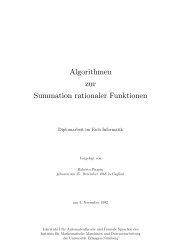
Figure 7.4: real part <strong>of</strong> C 1⋆,z (left),<br />
real part <strong>of</strong> C 2⋆,z (right)<br />
Hence, the dimension <strong>of</strong> the system is 10. Finally, we take two particular <strong>curves</strong> in<br />
the system, C 1 and C 2 , defined by the polynomials:<br />
H 1 (x, y, z) = 3 y 3 z 2 − 6 y 4 z + 3 y 5 − xy 3 z + xy 4 − 5 x 2 y z 2 + 2 x 2 y 2 z + x 3 y 2<br />
+x 4 z + y x 4 ,<br />
H 2 (x, y, z) = y 3 z 2 − 2 y 4 z + y 5 − 8 3 z2 xy 2 + 3 xy 3 z − 1 3 xy4 − 8 x 2 y z 2 + 2 x 2 y 2 z<br />
+y 3 x 2 + 2 y x 3 z + x 3 y 2 − x 4 z + 2 y x 4 + x 5 ,<br />
respectively. In the figure the real part <strong>of</strong> the affine <strong>curves</strong> C 1⋆,z and C 2⋆,z are plotted,<br />
respectively.<br />
Theorem 7.3.1. If two <strong>curves</strong> F 1 , F 2 ∈ S n have n 2 points in common, and exactly<br />
mn <strong>of</strong> these lie on an irreducible curve <strong>of</strong> degree m, then the other n(n − m) common<br />
points lie on a curve <strong>of</strong> degree n − m.<br />
Pro<strong>of</strong>: Let G be an irreducible curve <strong>of</strong> degree m containing exactly mn <strong>of</strong> the n 2<br />
common points <strong>of</strong> F 1 and F 2 . We choose an additional point P on G and determine a<br />
curve F in the system<br />
λ 1 F 1 + λ 2 F 2 = 0<br />
containing P. So F = λ 1 F 1 +λ 2 F 2 , for some λ 1 , λ 2 ∈ K. G and F have at least mn+1<br />
points in common, so by Theorem 7.2.2 (Bézout’s Theorem) they must have a common<br />
106
component, which must be G, since G is irreducible. F = G ·H contains the n 2 points,<br />
so the curve H ∈ S n−m contains the n(n − m) points not on G.<br />
As a special case we get Pascal’s Theorem.<br />
Theorem 7.3.2. (Pascal’s Theorem) Let C be an irreducible conic (curve <strong>of</strong> degree<br />
2). The opposite sides <strong>of</strong> a hexagon inscribed in C meet in 3 collinear points.<br />
Pro<strong>of</strong>: Let P 1 , . . ., P 6 be different points on C. Let L i be the line through P i and P i+1<br />
for 1 ≤ i ≤ 6 (for this we set P 7 = P 1 ). The 2 cubic <strong>curves</strong> L 1 L 3 L 5 and L 2 L 4 L 6 meet<br />
in the 6 vertices <strong>of</strong> the hexagon and in the 3 intersection points <strong>of</strong> opposite sides. The<br />
6 vertices lie on an irreducible conic, so by Theorem 7.3.1 the remaining 3 points must<br />
lie on a line.<br />
Example 7.3.3. Consider the following particular example <strong>of</strong> Pascal’s Theorem:<br />
Now we want to apply these results for deriving bounds for the number <strong>of</strong> singularities<br />
on <strong>plane</strong> <strong>algebraic</strong> <strong>curves</strong>.<br />
Theorem 7.3.3. Let F, G be <strong>curves</strong> <strong>of</strong> degree m, n, respectively, having no common<br />
components and having the multiplicities r 1 , . . .,r k and s 1 , . . ., s k in their common<br />
points P 1 , . . ., P k , respectively. Then<br />
k∑<br />
r i s i ≤ mn.<br />
i=1<br />
Pro<strong>of</strong>: The statement follows from Theorem 7.2.2 (Bézout’s Theorem) and proposition<br />
(5) in Theorem 7.2.3.<br />
107
Theorem 7.3.4. Let the curve F <strong>of</strong> degree n have no multiple components and let<br />
P 1 , . . .,P m be the singularities <strong>of</strong> F with multiplicities r 1 , . . .,r m , respectively. Then<br />
n(n − 1) ≥<br />
m∑<br />
r i (r i − 1).<br />
i=1<br />
Pro<strong>of</strong>: Choose the coordinate system such that the point (0 : 0 : 1) is not contained<br />
in F (i.e. the term z n occurs with non-zero coefficient in F). Then<br />
F z (x, y, z) := ∂F<br />
∂z ≠ 0.<br />
Moreover, F does not have a factor independent <strong>of</strong> z. Since F is squarefree, F can<br />
have no factor in common with F z .<br />
The curve F z has every point P i as a point <strong>of</strong> multiplicity at least r i −1, since every<br />
j–th derivative <strong>of</strong> F z is a (j + 1)-st derivative <strong>of</strong> F. Thus, by application <strong>of</strong> Theorem<br />
7.3.3 we get the result.<br />
This bound can be sharpened even more for irreducible <strong>curves</strong>.<br />
Theorem 7.3.5. Let the irreducible curve F <strong>of</strong> degree n have the singularities<br />
P 1 , . . .,P m <strong>of</strong> multiplicities r 1 , . . ., r m , respectively. Then<br />
(n − 1)(n − 2) ≥<br />
m∑<br />
r i (r i − 1).<br />
i=1<br />
Pro<strong>of</strong>: From Theorem 7.3.4 we get<br />
∑<br />
ri (r i − 1)<br />
≤<br />
2<br />
n(n − 1)<br />
2<br />
≤<br />
(n − 1)(n + 2)<br />
.<br />
2<br />
(Note: one can always determine a curve <strong>of</strong> degree n − 1 satisfying (n − 1)(n + 2)/2<br />
linear conditions. By r(r − 1)/2 linear conditions we can force a point P to be an<br />
(r − 1)–fold point on a curve.)<br />
So, there is a curve G <strong>of</strong> degree n − 1 having P i as (r i − 1)–fold point, 1 ≤ i ≤ m,<br />
and additionally passing through<br />
(n − 1)(n + 2)<br />
2<br />
−<br />
∑<br />
ri (r i − 1)<br />
simple points <strong>of</strong> F. Since F is irreducible and deg(G) < deg(F), the <strong>curves</strong> F and G<br />
can have no common component. Therefore, by Theorem 7.3.3,<br />
2<br />
n(n − 1) ≥ ∑ r i (r i − 1) +<br />
(n − 1)(n + 2)<br />
2<br />
−<br />
∑<br />
ri (r i − 1)<br />
,<br />
2<br />
108
and consequently<br />
(n − 1)(n − 2) ≥ ∑ r i (r i − 1).<br />
Indeed, the bound in Theorem 7.3.5 is sharp, i.e. it is actually achieved by a certain<br />
class <strong>of</strong> irreducible <strong>curves</strong>. These are the <strong>curves</strong> <strong>of</strong> genus 0.<br />
Definition 7.3.4. Let F be an irreducible curve <strong>of</strong> degree n, having only ordinary<br />
singularities <strong>of</strong> multiplicities r 1 , . . .,r m . The genus <strong>of</strong> F, genus(F), is defined as<br />
genus(F) = 1 m<br />
[(n − 1)(n − 2) −<br />
2<br />
∑<br />
r i (r i − 1)].<br />
i=1<br />
Example 7.3.4. Every irreducible conic has genus 0. An irreducible cubic has genus<br />
0 if and only if it has a double point.<br />
For <strong>curves</strong> with non-ordinary singularities the formula<br />
m<br />
1<br />
2 [(n − 1)(n − 2) − ∑<br />
r i (r i − 1)]<br />
is just an upper bound for the genus. Compare the tacnode curve <strong>of</strong> Example 1.3,<br />
which is a curve <strong>of</strong> genus 0. We will see this in the chapter on parametrization.<br />
i=1<br />
109