Advances in Intelligent Systems Research - of Marcus Hutter
Advances in Intelligent Systems Research - of Marcus Hutter
Advances in Intelligent Systems Research - of Marcus Hutter

Create successful ePaper yourself
Turn your PDF publications into a flip-book with our unique Google optimized e-Paper software.
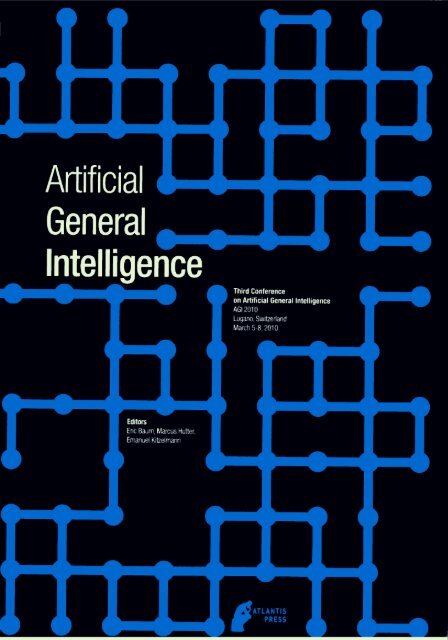
Eric Baum, <strong>Marcus</strong> <strong>Hutter</strong>, Emanuel Kitzelmann (Editors)<br />
Artificial General Intelligence<br />
Proceed<strong>in</strong>gs <strong>of</strong> the Third Conference on Artificial General<br />
Intelligence, AGI 2010, Lugano, Switzerland, March 5-8, 2010<br />
Amsterdam-Beij<strong>in</strong>g-Paris<br />
ISBN: 978-90-78677-36-9
________________________________________________________________________<br />
<strong>Advances</strong> <strong>in</strong> <strong>Intelligent</strong> <strong>Systems</strong> <strong>Research</strong><br />
volume 10<br />
________________________________________________________________________
In Memoriam<br />
Ray Solomon<strong>of</strong>f (1926-2009)<br />
The Great Ray Solomon<strong>of</strong>f, pioneer <strong>of</strong> Mach<strong>in</strong>e Learn<strong>in</strong>g, founder <strong>of</strong> Algorithmic Probability<br />
Theory, father <strong>of</strong> the Universal Probability Distribution, creator <strong>of</strong> the Universal Theory <strong>of</strong> Inductive<br />
Inference, passed away on Monday 30 November 2009, from complications <strong>in</strong> the wake <strong>of</strong> a broken<br />
aneurism <strong>in</strong> his head. He is survived by his lov<strong>in</strong>g wife, Grace.<br />
Ray Solomon<strong>of</strong>f was the first to describe the fundamental concept <strong>of</strong> Algorithmic Information or<br />
Kolmogorov Complexity, and the first to prove the celebrated Invariance Theorem. In the new millennium<br />
his work became the foundation <strong>of</strong> the first mathematical theory <strong>of</strong> Optimal Universal Artificial Intelligence.<br />
Ray <strong>in</strong>tended to deliver an <strong>in</strong>vited lecture at AGI 2010, the Conference on Artificial General<br />
Intelligence (March 5-8, 2010) <strong>in</strong> Lugano (where he already spent time <strong>in</strong> 2001 as a visit<strong>in</strong>g pr<strong>of</strong>essor at the<br />
Swiss AI Lab IDSIA). The AGI conference series would not even exist without his essential theoretical<br />
contributions. With great sadness AGI 2010 was held «In Memoriam Ray Solomon<strong>of</strong>f».<br />
Ray will live on <strong>in</strong> the many m<strong>in</strong>ds shaped by his revolutionary ideas.<br />
Eulogy by Jürgen Schmidhuber
This book is part <strong>of</strong> the series <strong>Advances</strong> <strong>in</strong> <strong>Intelligent</strong> <strong>Systems</strong> <strong>Research</strong> (ISSN: 1951-6851) published by<br />
Atlantis Press.<br />
Aims and scope <strong>of</strong> the series<br />
Dur<strong>in</strong>g the past decade computer science research <strong>in</strong> understand<strong>in</strong>g and reproduc<strong>in</strong>g human <strong>in</strong>telligence has<br />
expanded from the more traditional approaches like psychology, logics and artificial <strong>in</strong>telligence <strong>in</strong>to<br />
multiple other areas, <strong>in</strong>clud<strong>in</strong>g neuroscience research. Moreover, new results <strong>in</strong> biology, chemistry, (surface)<br />
physics and gene technology, but also <strong>in</strong> network technology are greatly affect<strong>in</strong>g current research <strong>in</strong><br />
computer science, <strong>in</strong>clud<strong>in</strong>g the development <strong>of</strong> <strong>in</strong>telligent systems. At the same time, computer science’s<br />
new results are <strong>in</strong>creas<strong>in</strong>gly be<strong>in</strong>g applied <strong>in</strong> these fields allow<strong>in</strong>g for important cross-fertilisations. This<br />
series aims at publish<strong>in</strong>g proceed<strong>in</strong>gs from all discipl<strong>in</strong>es deal<strong>in</strong>g with and affect<strong>in</strong>g the issue <strong>of</strong><br />
understand<strong>in</strong>g and reproduc<strong>in</strong>g <strong>in</strong>telligence <strong>in</strong> artificial systems. Also, the series is open for publications<br />
concern<strong>in</strong>g the application <strong>of</strong> <strong>in</strong>telligence <strong>in</strong> networked or any other environment and the extraction <strong>of</strong><br />
mean<strong>in</strong>gful data from large data sets.<br />
<strong>Research</strong> fields covered by the series <strong>in</strong>clude: * Fuzzy sets * Mach<strong>in</strong>e learn<strong>in</strong>g * Autonomous agents *<br />
Evolutionary systems * Robotics and autonomous systems * Semantic web, <strong>in</strong>cl. web services, ontologies<br />
and grid comput<strong>in</strong>g * Biological systems * Artificial Intelligence, <strong>in</strong>cl. knowledge representation, logics *<br />
Neural networks * Constra<strong>in</strong>t satisfaction * Computational biology * Information sciences * Computer<br />
vision, pattern recognition * Computational neuroscience * Datam<strong>in</strong><strong>in</strong>g, knowledge discovery and modell<strong>in</strong>g<br />
for e.g. life sciences.<br />
© ATLANTIS PRESS, 2010<br />
http://www.atlantis-press.com<br />
ISBN: 978-90-78677-36-9<br />
This book is published by Atlantis Press, scientific publish<strong>in</strong>g, Paris, France.<br />
All rights reserved for this book. No part <strong>of</strong> this book may be reproduced, translated, stored or transmitted <strong>in</strong><br />
any form or by any means, <strong>in</strong>clud<strong>in</strong>g electronic, mechanical, photocopy<strong>in</strong>g, record<strong>in</strong>g or otherwise, without<br />
prior permission from the publisher.<br />
Atlantis Press adheres to the creative commons policy, which means that authors reta<strong>in</strong> the copyright <strong>of</strong> their<br />
article.
Artificial General Intelligence<br />
Volume Editors<br />
<strong>Marcus</strong> <strong>Hutter</strong><br />
CSL@RSISE and SML@NICTA<br />
Australian National University<br />
Room B259, Build<strong>in</strong>g 115<br />
Corner <strong>of</strong> North and Daley Road<br />
Canberra ACT 0200, Australia<br />
Email: marcus.hutter@gmx.net<br />
WWW: http://www.hutter1.net<br />
Eric B. Baum<br />
Azure Sky <strong>Research</strong> Inc.<br />
386 Riverside Drive<br />
Pr<strong>in</strong>ceton NJ 08540 USA<br />
Email: ebaum@fastmail.fm<br />
WWW: http://whatisthought.com/<br />
Emanuel Kitzelmann<br />
Cognitive <strong>Systems</strong> Group, WIAI<br />
University <strong>of</strong> Bamberg<br />
Feldkirchenstrasse 21<br />
D-96052 Bamberg, Germany<br />
Email: emanuel.kitzelmann@uni-bamberg.de<br />
WWW: http://www.uni-bamberg.de/kogsys/members/kitzelmann/
Preface<br />
Artificial General Intelligence (AGI) research focuses on the orig<strong>in</strong>al and ultimate goal <strong>of</strong> AI - to create<br />
broad human-like and transhuman <strong>in</strong>telligence, by explor<strong>in</strong>g all available paths, <strong>in</strong>clud<strong>in</strong>g theoretical and<br />
experimental computer science, cognitive science, neuroscience, and <strong>in</strong>novative <strong>in</strong>terdiscipl<strong>in</strong>ary<br />
methodologies. Due to the difficulty <strong>of</strong> this task, for the last few decades the majority <strong>of</strong> AI researchers have<br />
focused on what has been called narrow AI - the production <strong>of</strong> AI systems display<strong>in</strong>g <strong>in</strong>telligence regard<strong>in</strong>g<br />
specific, highly constra<strong>in</strong>ed tasks. In recent years, however, more and more researchers have recognized the<br />
necessity - and feasibility - <strong>of</strong> return<strong>in</strong>g to the orig<strong>in</strong>al goals <strong>of</strong> the field. Increas<strong>in</strong>gly, there is a call for a<br />
transition back to confront<strong>in</strong>g the more difficult issues <strong>of</strong> human level <strong>in</strong>telligence and more broadly<br />
artificial general <strong>in</strong>telligence.<br />
The Conference on Artificial General Intelligence is the only major conference series devoted wholly<br />
and specifically to the creation <strong>of</strong> AI systems possess<strong>in</strong>g general <strong>in</strong>telligence at the human level and<br />
ultimately beyond. Its third <strong>in</strong>stallation, AGI-10, <strong>in</strong> Lugano, Switzerland, March 5-8, 2010, attracted 66<br />
paper submissions. Of these submissions, 29 (i.e., 44%) were accepted as full papers, additional 12 were<br />
accepted as short position papers, which was a more selective choice than for AGI-09 <strong>in</strong> Arl<strong>in</strong>gton, Virg<strong>in</strong>ia.<br />
Both full and short papers are <strong>in</strong>cluded <strong>in</strong> this collection. The papers presented at the conference and<br />
collected <strong>in</strong> these proceed<strong>in</strong>gs address a wide range <strong>of</strong> AGI-related topics such as Universal Search,<br />
Cognitive and AGI Architectures, Adaptive Agents, special aspects <strong>of</strong> reason<strong>in</strong>g, the formalization <strong>of</strong> AGI,<br />
the evaluation <strong>of</strong> AGI systems, mach<strong>in</strong>e learn<strong>in</strong>g for AGI, and implications <strong>of</strong> AGI. The contributions range<br />
from proven theoretical results to system descriptions, implementations, and experiments to general ideas<br />
and visions.<br />
The conference program also <strong>in</strong>cluded a keynote address by Richard Sutton and an <strong>in</strong>vited lecture by<br />
Randal Koene. Richard Sutton is a Pr<strong>of</strong>essor at the University <strong>of</strong> Alberta. The co-author <strong>of</strong> the textbook<br />
«Re<strong>in</strong>forcement Learn<strong>in</strong>g: an Introduction», has made numerous contributions to the fields <strong>of</strong> AI and<br />
learn<strong>in</strong>g. His talk was on Reduc<strong>in</strong>g Knowledge to Prediction. The idea is to formalize and reduce knowledge<br />
about the world to predictive statements <strong>of</strong> a particular form that is particularly well suited for learn<strong>in</strong>g and<br />
reason<strong>in</strong>g. He presented new learn<strong>in</strong>g algorithms <strong>in</strong> this framework that his research group has developed.<br />
Randal Koene is the Director <strong>of</strong> the Department <strong>of</strong> Neuroeng<strong>in</strong>eer<strong>in</strong>g at Tecnalia. His talk was on Whole<br />
Bra<strong>in</strong> Emulation: Issues <strong>of</strong> scope and resolution, and the need for new methods <strong>of</strong> <strong>in</strong>-vivo record<strong>in</strong>g.<br />
F<strong>in</strong>ally, the conference program <strong>in</strong>cluded a number <strong>of</strong> workshops on topics such as formaliz<strong>in</strong>g AGI<br />
and the future <strong>of</strong> AI, pre-conference tutorials on various AGI-related topics, and an AGI-systems<br />
demonstration.<br />
Produc<strong>in</strong>g such a highly pr<strong>of</strong>iled program would not have been possible without the support <strong>of</strong> the<br />
community. We thank the (local) organiz<strong>in</strong>g committee members for their advise and their help <strong>in</strong> all matters<br />
<strong>of</strong> actually prepar<strong>in</strong>g and runn<strong>in</strong>g the event. We thank the program committee members for a smooth review<br />
process and for the high quality <strong>of</strong> the reviews - despite the tight review phase and the fact that due to the<br />
high number <strong>of</strong> submissions the review load per PC member was considerably higher than orig<strong>in</strong>ally<br />
expected. And we thank all participants for submitt<strong>in</strong>g and present<strong>in</strong>g <strong>in</strong>terest<strong>in</strong>g and stimulat<strong>in</strong>g work,<br />
which is the key <strong>in</strong>gredient needed for a successful conference. We also gratefully acknowledge the support<br />
<strong>of</strong> a number <strong>of</strong> sponsors:<br />
• Association for the Advancement <strong>of</strong> Artificial Intelligence (AAAI)<br />
• KurzweilAI.net (Kurzweil Best Paper Prize and Kurzweil Best Idea Prize)<br />
• The University <strong>of</strong> Lugano, Faculty <strong>of</strong> Informatics (scientifically endorses AGI-10)<br />
March 2010<br />
<strong>Marcus</strong> <strong>Hutter</strong> (Conference Chair)<br />
Eric Baum, Emanuel Kitzelmann (Program Committee Chairs)
Conference Organization<br />
Chairs<br />
<strong>Marcus</strong> <strong>Hutter</strong> (Conference Chair)<br />
Jürgen Schmidhuber (Local Chair)<br />
Eric Baum (Program Chair)<br />
Emanuel Kitzelmann (Program Chair)<br />
Australian National University, Australia<br />
IDSIA, Switzerland<br />
Azure Sky <strong>Research</strong> Inc., USA<br />
University <strong>of</strong> Bamberg, Germany<br />
Program Committee<br />
Igor Aleksander<br />
Imperial College London, UK<br />
Lee Altenberg<br />
University <strong>of</strong> Hawaii at Manoa, USA<br />
Itamar Arel<br />
University <strong>of</strong> Tennessee, Knoxville, USA<br />
Sebastian Bader<br />
Rostock University, Germany<br />
Eric Baum<br />
Azure Sky <strong>Research</strong> Inc., USA<br />
Anselm Blumer<br />
Tufts University, USA<br />
Hugo de Garis<br />
Xiamen University, Ch<strong>in</strong>a<br />
Wlodek Duch<br />
Nicolaus Copernicus University, Poland<br />
Artur Garcez<br />
City University London, UK<br />
J. Storrs Hall Institute for Molecular Manufactur<strong>in</strong>g, USA<br />
Benjam<strong>in</strong> Johnston<br />
University <strong>of</strong> Technology, Sydney, Australia<br />
Bert Kappen<br />
Radboud University, The Netherlands<br />
Emanuel Kitzelmann<br />
University <strong>of</strong> Bamberg, Germany<br />
Kai-Uwe Kühnberger<br />
University <strong>of</strong> Osnabrück, Germany<br />
Christian Lebiere<br />
Carnegie Mellon University, USA<br />
Shane Legg<br />
University College London, UK<br />
Moshe Looks<br />
Google <strong>Research</strong>, USA<br />
András Lör<strong>in</strong>cz<br />
Eötvös Loránd University, Hungary<br />
Hassan Mahmud<br />
Australian National University, Australia<br />
Eric Nivel<br />
Reykjavik University, Iceland<br />
Jan Poland<br />
ABB <strong>Research</strong>, Zurich, Switzerland<br />
Brandon Rohrer<br />
Sandia National Laboratory, USA<br />
Sebastian Rudolph<br />
University <strong>of</strong> Karlsruhe, Germany<br />
Robert Schapire<br />
Pr<strong>in</strong>ceton University, USA<br />
Lokendra Shastri<br />
Infosys Technologies Ltd, India<br />
Ray Solomono<br />
Oxbridge <strong>Research</strong>, Cambridge, USA<br />
Rich Sutton<br />
University <strong>of</strong> Alberta, Canada<br />
Krist<strong>in</strong>n Thorisson<br />
Reykjavik University, Iceland
Lyle Ungar<br />
Les Valiant<br />
Marco Wier<strong>in</strong>g<br />
Mary-Anne Williams<br />
David Wolpert<br />
University <strong>of</strong> Pennsylvania, USA<br />
Harvard University, USA<br />
University <strong>of</strong> Gron<strong>in</strong>gen, The Netherlands<br />
University <strong>of</strong> Technology, Sydney, Australia<br />
NASA, USA<br />
Organiz<strong>in</strong>g Committee<br />
Tsvi Achler<br />
Eric Baum<br />
Sarah Bull<br />
Ben Goertzel<br />
<strong>Marcus</strong> <strong>Hutter</strong><br />
Emanuel Kitzelmann<br />
David Orban<br />
Stephen Reed<br />
University <strong>of</strong> Ill<strong>in</strong>ois at Urbana Champaign, USA<br />
Azure Sky <strong>Research</strong> Inc., USA<br />
NICTA, Australia<br />
Novamente LLC, USA<br />
Australian National University, Australia<br />
University <strong>of</strong> Bamberg, Germany<br />
S<strong>in</strong>gularity University, USA<br />
Texai.org, USA<br />
Local Organiz<strong>in</strong>g Committee<br />
Carlo Lepori<br />
Mauro Pezze<br />
Jürgen Schmidhuber<br />
Alb<strong>in</strong>o Zgraggen<br />
CFO <strong>of</strong> IDSIA<br />
Dean <strong>of</strong> the Faculty <strong>of</strong> Informatics <strong>of</strong> USI<br />
IDSIA<br />
CFO <strong>of</strong> the University <strong>of</strong> Lugano/USI<br />
External Reviewers<br />
Subhadip Bandyopadhyay<br />
Arijit Laha<br />
Sr<strong>in</strong>ivas Narasimhamurthy<br />
B<strong>in</strong>tu Vasudevan
Table <strong>of</strong> Contents<br />
Full Articles.<br />
Efficient Constra<strong>in</strong>t-Satisfaction <strong>in</strong> Doma<strong>in</strong>s with Time . . . . . . . . . . . . . . . . . . . . . . . . . . . . . . 1<br />
Perr<strong>in</strong> Bignoli, Nicholas Cassimatis, Arthi Murugesan<br />
The CHREST Architecture <strong>of</strong> Cognition: The Role <strong>of</strong> Perception <strong>in</strong> General Intelligence . 7<br />
Fernand Gobet, Peter Lane<br />
A General Intelligence Oriented Architecture for Embodied Natural Language Process<strong>in</strong>g 13<br />
Ben Goertzel, Cassio Pennach<strong>in</strong>, Samir Araujo, Ruit<strong>in</strong>g Lian, Fabricio Silva, Murilo<br />
Queiroz, Welter Silva, Mike Ross, L<strong>in</strong>as Vepstas, Andre Senna<br />
Toward a Formal Characterization <strong>of</strong> Real-World General Intelligence . . . . . . . . . . . . . . . . . 19<br />
Ben Goertzel<br />
On Evaluat<strong>in</strong>g Agent Performance <strong>in</strong> a Fixed Period <strong>of</strong> Time . . . . . . . . . . . . . . . . . . . . . . . . . 25<br />
Jose Hernandez-Orallo<br />
Artificial General Segmentation . . . . . . . . . . . . . . . . . . . . . . . . . . . . . . . . . . . . . . . . . . . . . . . . . . . 31<br />
Daniel Hewlett, Paul Cohen<br />
Ground<strong>in</strong>g Possible Worlds Semantics <strong>in</strong> Experiential Semantics . . . . . . . . . . . . . . . . . . . . . . 37<br />
Matthew Ikle, Ben Goertzel<br />
The Toy Box Problem (and a Prelim<strong>in</strong>ary Solution) . . . . . . . . . . . . . . . . . . . . . . . . . . . . . . . . . 43<br />
Benjam<strong>in</strong> Johnston<br />
Play<strong>in</strong>g General Structure Rewrit<strong>in</strong>g Games . . . . . . . . . . . . . . . . . . . . . . . . . . . . . . . . . . . . . . . . 49<br />
Lukasz Kaiser, Lukasz Staf<strong>in</strong>iak<br />
Towards Automated Code Generation for Autonomous Mobile Robots . . . . . . . . . . . . . . . . . 55<br />
Dermot Kerr, Ulrich Nehmzow, Stephen A. Bill<strong>in</strong>gs<br />
Search<strong>in</strong>g for M<strong>in</strong>imal Neural Networks <strong>in</strong> Fourier Space . . . . . . . . . . . . . . . . . . . . . . . . . . . . . 61<br />
Jan Koutnik, Faust<strong>in</strong>o Gomez, Juergen Schmidhuber<br />
Remarks on the Mean<strong>in</strong>g <strong>of</strong> Analogical Relations. . . . . . . . . . . . . . . . . . . . . . . . . . . . . . . . . . . . 67<br />
Ulf Krumnack, Helmar Gust, Angela Schwer<strong>in</strong>g, Kai-Uwe Kuehnberger<br />
Quantitative Spatial Reason<strong>in</strong>g for General Intelligence . . . . . . . . . . . . . . . . . . . . . . . . . . . . . . 73<br />
Unmesh Kurup, Nicholas Cassimatis<br />
Cognitive Architecture Requirements for Achiev<strong>in</strong>g AGI . . . . . . . . . . . . . . . . . . . . . . . . . . . . . 79<br />
John Laird, Robert Wray<br />
Sketch <strong>of</strong> an AGI Architecture with Illustration . . . . . . . . . . . . . . . . . . . . . . . . . . . . . . . . . . . . . 85<br />
Andras Lor<strong>in</strong>cz, Zoltan Bardosi, Daniel Takacs
GQ(λ): A General Gradient Algorithm for Temporal-Difference Prediction Learn<strong>in</strong>g<br />
with Eligibility Traces . . . . . . . . . . . . . . . . . . . . . . . . . . . . . . . . . . . . . . . . . . . . . . . . . . . . . . . . . . . 91<br />
Hamid Maei, Richard Sutton<br />
A Generic Adaptive Agent Architecture Integrat<strong>in</strong>g Cognitive and Affective States and<br />
their Interaction . . . . . . . . . . . . . . . . . . . . . . . . . . . . . . . . . . . . . . . . . . . . . . . . . . . . . . . . . . . . . . . . 97<br />
Zulfiqar A. Memon, Jan Treur<br />
A Cognitive Architecture for Knowledge Exploitation . . . . . . . . . . . . . . . . . . . . . . . . . . . . . . . . 103<br />
Gee Wah Ng, Yuan S<strong>in</strong> Tan, Loo N<strong>in</strong> Teow, Kh<strong>in</strong> Hua Ng, Kheng Hwee Tan, Rui Zhong<br />
Chan<br />
An Artificial Intelligence Model that Comb<strong>in</strong>es Spatial and Temporal Perception . . . . . . . . 109<br />
Jianglong Nan, F<strong>in</strong>tan Costello<br />
A Conversion Between Utility and Information . . . . . . . . . . . . . . . . . . . . . . . . . . . . . . . . . . . . . 115<br />
Pedro Ortega, Daniel Braun<br />
A Bayesian Rule for Adaptive Control based on Causal Interventions . . . . . . . . . . . . . . . . . . 121<br />
Pedro Ortega, Daniel Braun<br />
Discover<strong>in</strong>g and Characteriz<strong>in</strong>g Hidden Variables . . . . . . . . . . . . . . . . . . . . . . . . . . . . . . . . . . . 127<br />
Soumi Ray, Tim Oates<br />
What we Might Look for <strong>in</strong> an AGI Benchmark . . . . . . . . . . . . . . . . . . . . . . . . . . . . . . . . . . . . . 133<br />
Brandon Rohrer<br />
Towards Practical Universal Search . . . . . . . . . . . . . . . . . . . . . . . . . . . . . . . . . . . . . . . . . . . . . . . 139<br />
Tom Schaul, Juergen Schmidhuber<br />
Artificial Scientists & Artists Based on the Formal Theory <strong>of</strong> Creativity . . . . . . . . . . . . . . . 145<br />
Juergen Schmidhuber<br />
Algorithmic Probability, Heuristic Programm<strong>in</strong>g and AGI . . . . . . . . . . . . . . . . . . . . . . . . . . . . 151<br />
Ray Solomon<strong>of</strong>f<br />
Frontier Search . . . . . . . . . . . . . . . . . . . . . . . . . . . . . . . . . . . . . . . . . . . . . . . . . . . . . . . . . . . . . . . . . 158<br />
Yi Sun, Tobias Glasmachers, Tom Schaul, Juergen Schmidhuber<br />
The Evaluation <strong>of</strong> AGI <strong>Systems</strong> . . . . . . . . . . . . . . . . . . . . . . . . . . . . . . . . . . . . . . . . . . . . . . . . . . . 164<br />
Pei Wang<br />
Design<strong>in</strong>g a Safe Motivational System for <strong>Intelligent</strong> Mach<strong>in</strong>es . . . . . . . . . . . . . . . . . . . . . . . . 170<br />
Mark Waser<br />
Position Statements.<br />
S<strong>of</strong>tware Design <strong>of</strong> an AGI System Based on Perception Loop . . . . . . . . . . . . . . . . . . . . . . . . 176<br />
Antonio Chella, Massimo Cossent<strong>in</strong>o, Valeria Seidita<br />
A Theoretical Framework to Formalize AGI-Hard Problems . . . . . . . . . . . . . . . . . . . . . . . . . . 178<br />
Pedro Demasi, Jayme Szwarcfiter, Adriano Cruz
Uncerta<strong>in</strong> Spatiotemporal Logic for General Intelligence . . . . . . . . . . . . . . . . . . . . . . . . . . . . . 180<br />
Nil Geisweiller, Ben Goertzel<br />
A (hopefully) Unbiased Universal Environment Class for Measur<strong>in</strong>g Intelligence <strong>of</strong><br />
Biological and Artificial <strong>Systems</strong> . . . . . . . . . . . . . . . . . . . . . . . . . . . . . . . . . . . . . . . . . . . . . . . . . . 182<br />
Jose Hernandez-Orallo<br />
Neuroethological Approach to Understand<strong>in</strong>g Intelligence . . . . . . . . . . . . . . . . . . . . . . . . . . . . 184<br />
DaeEun Kim<br />
Compression Progress, Pseudorandomness, and Hyperbolic Discount<strong>in</strong>g . . . . . . . . . . . . . . . . 186<br />
Moshe Looks<br />
Relational Local Iterative Compression . . . . . . . . . . . . . . . . . . . . . . . . . . . . . . . . . . . . . . . . . . . . 188<br />
Laurent Orseau<br />
Stochastic Grammar Based Incremental Mach<strong>in</strong>e Learn<strong>in</strong>g Us<strong>in</strong>g Scheme . . . . . . . . . . . . . . 190<br />
Eray Ozkural, Cevdet Aykanat<br />
Compression-driven Progress <strong>in</strong> Science . . . . . . . . . . . . . . . . . . . . . . . . . . . . . . . . . . . . . . . . . . . . 192<br />
Leo Pape<br />
Concept Formation <strong>in</strong> the Ouroboros Model . . . . . . . . . . . . . . . . . . . . . . . . . . . . . . . . . . . . . . . . 194<br />
Knud Thomsen<br />
On Super-Tur<strong>in</strong>g Comput<strong>in</strong>g Power and Hierarchies <strong>of</strong> Artificial General Intelligence<br />
<strong>Systems</strong> . . . . . . . . . . . . . . . . . . . . . . . . . . . . . . . . . . . . . . . . . . . . . . . . . . . . . . . . . . . . . . . . . . . . . . . 196<br />
Jiri Wiedermann<br />
A M<strong>in</strong>imum Relative Entropy Pr<strong>in</strong>ciple for AGI . . . . . . . . . . . . . . . . . . . . . . . . . . . . . . . . . . . . 198<br />
Anto<strong>in</strong>e van de Ven, Ben Schouten<br />
Author Index . . . . . . . . . . . . . . . . . . . . . . . . . . . . . . . . . . . . . . . . . . . . . . . . . . . . . . . . . . . . . . . . . 200
Efficient Constra<strong>in</strong>t-Satisfaction <strong>in</strong> Doma<strong>in</strong>s with Time<br />
Perr<strong>in</strong> G. Bignoli, Nicholas L. Cassimatis, Arthi Murugesan<br />
Department <strong>of</strong> Cognitive Science<br />
Rensselaer Polytechnic Institute<br />
Troy, NY 12810<br />
{bignop, cass<strong>in</strong>, muruga}@rpi.edu<br />
Abstract<br />
Satisfiability (SAT) test<strong>in</strong>g methods have been used<br />
effectively <strong>in</strong> many <strong>in</strong>ference, plann<strong>in</strong>g and constra<strong>in</strong>t<br />
satisfaction tasks and thus have been considered a<br />
contribution towards artificial general <strong>in</strong>telligence.<br />
However, s<strong>in</strong>ce SAT constra<strong>in</strong>ts are def<strong>in</strong>ed over atomic<br />
propositions, doma<strong>in</strong>s with state variables that change over<br />
time can lead to extremely large search spaces. This poses<br />
both memory- and time-efficiency problems for exist<strong>in</strong>g<br />
SAT algorithms. In this paper, we propose to address these<br />
problems by <strong>in</strong>troduc<strong>in</strong>g a language that encodes the<br />
temporal <strong>in</strong>tervals over which relations occur and an<br />
<strong>in</strong>tegrated system that satisfies constra<strong>in</strong>ts formulated <strong>in</strong> this<br />
language. Temporal <strong>in</strong>tervals are presented as a compressed<br />
method <strong>of</strong> encod<strong>in</strong>g time that results <strong>in</strong> significantly smaller<br />
search spaces. However, <strong>in</strong>tervals cannot be used efficiently<br />
without significant modifications to traditional SAT<br />
algorithms. Us<strong>in</strong>g the Polyscheme cognitive architecture,<br />
we created a system that <strong>in</strong>tegrates a DPLL-like SATsolv<strong>in</strong>g<br />
algorithm with a rule matcher <strong>in</strong> order to support<br />
<strong>in</strong>tervals by allow<strong>in</strong>g new constra<strong>in</strong>ts and objects to be<br />
lazily <strong>in</strong>stantiated throughout <strong>in</strong>ference. Our system also<br />
<strong>in</strong>cludes constra<strong>in</strong>t graphs to compactly store <strong>in</strong>formation<br />
about temporal and identity relationships between objects.<br />
In addition, a memory retrieval subsystem was utilized to<br />
guide <strong>in</strong>ference towards m<strong>in</strong>imal models <strong>in</strong> common sense<br />
reason<strong>in</strong>g problems <strong>in</strong>volv<strong>in</strong>g time and change. We<br />
performed two sets <strong>of</strong> evaluations to isolate the<br />
contributions <strong>of</strong> the system‟s <strong>in</strong>dividual components. These<br />
tests demonstrate that both the ability to add new objects<br />
dur<strong>in</strong>g <strong>in</strong>ference and the use <strong>of</strong> smart memory retrieval<br />
result <strong>in</strong> a significant <strong>in</strong>crease <strong>in</strong> performance over pure<br />
satisfiability algorithms alone and <strong>of</strong>fer solutions to some<br />
problems on a larger scale than what was possible before.<br />
Introduction<br />
Many AI applications have been successfully framed as<br />
SAT problems: plann<strong>in</strong>g (Kautz and Selman 1999),<br />
computer-aided design (Marques-Silva and Sakallah 2000),<br />
diagnosis (Smith and Veneris 2005), and schedul<strong>in</strong>g<br />
(Feldman and Golumbic 1990). Although SAT-solvers<br />
have successfully handled problems with millions <strong>of</strong><br />
clauses, tasks that require an explicit representation <strong>of</strong> time<br />
can exceed their capacities.<br />
Add<strong>in</strong>g a temporal dimension to a problem space has the<br />
potential to greatly expand search space sizes because SAT<br />
algorithms propositionalize relational constra<strong>in</strong>ts. The most<br />
direct way to <strong>in</strong>corporate time is to have a copy <strong>of</strong> each<br />
state variable for every time po<strong>in</strong>t over which the system<br />
reasons. This <strong>in</strong>creases the number <strong>of</strong> propositions by a<br />
factor equal to the number <strong>of</strong> time po<strong>in</strong>ts <strong>in</strong>volved. S<strong>in</strong>ce<br />
SAT algorithms generally become slower as the size <strong>of</strong> a<br />
problem <strong>in</strong>creases, add<strong>in</strong>g a temporal dimension to even<br />
relatively simple problems can make them <strong>in</strong>tractable.<br />
Although problems with time require more space to<br />
encode, the true expense <strong>of</strong> <strong>in</strong>troduc<strong>in</strong>g time stems from<br />
the additional cost required to f<strong>in</strong>d a SAT solution.<br />
Consider a task that requires the comparison <strong>of</strong> all the<br />
possible ways that a car can visit three locations <strong>in</strong> order. If<br />
the problem has no reference to time po<strong>in</strong>ts, there is only<br />
one solution: the car just moves from a to b to c. On the<br />
other hand, there are clearly more possibilities, s<strong>in</strong>ce the<br />
car could potentially move or not move at every time.<br />
Compared to other SAT-solvers, LazySAT (S<strong>in</strong>gla and<br />
Dom<strong>in</strong>gos 2006), which lazily <strong>in</strong>stantiates constra<strong>in</strong>ts, is<br />
less affected by the <strong>in</strong>creased memory demands <strong>of</strong> larger<br />
search spaces. Unfortunately, lazy <strong>in</strong>stantiation will not<br />
<strong>in</strong>crease the tractability <strong>of</strong> larger problems with respect to<br />
runtime.<br />
There is, however, a more efficient way <strong>of</strong> represent<strong>in</strong>g<br />
time. S<strong>in</strong>ce it is unlikely that the truth value <strong>of</strong> a<br />
proposition will change at every time po<strong>in</strong>t, temporal<br />
<strong>in</strong>tervals can be used to denote segments <strong>of</strong> contiguous<br />
time po<strong>in</strong>ts over which its value is constant. This practice<br />
alleviates the need to duplicate all propositions at every<br />
time po<strong>in</strong>t for most problem <strong>in</strong>stances, thus significantly<br />
reduc<strong>in</strong>g the search space size. Intervals also mitigate the<br />
arbitrary granularity <strong>of</strong> time because they are cont<strong>in</strong>uous<br />
and scale <strong>in</strong>dependent.<br />
However, exist<strong>in</strong>g SAT solvers cannot process <strong>in</strong>tervals<br />
efficiently because they do not allow new objects to be<br />
<strong>in</strong>troduced dur<strong>in</strong>g the course <strong>of</strong> <strong>in</strong>ference. It is clearly<br />
impossible to know exactly which temporal <strong>in</strong>tervals will<br />
be required. Therefore, every possible <strong>in</strong>terval must be<br />
( n 1)(<br />
n 2)<br />
def<strong>in</strong>ed <strong>in</strong> advance. S<strong>in</strong>ce<br />
2<br />
unique <strong>in</strong>tervals can be<br />
def<strong>in</strong>ed over n times, there would be little advantage to use<br />
them with current search<strong>in</strong>g methods.<br />
To capture the benefits <strong>of</strong> SAT while support<strong>in</strong>g the use<br />
<strong>of</strong> <strong>in</strong>tervals, we created an <strong>in</strong>tegrated system that comb<strong>in</strong>es<br />
a DPLL-like search with several specialized forms <strong>of</strong><br />
<strong>in</strong>ference: a rule matcher, constra<strong>in</strong>t graphs, and memory<br />
retrieval. Rule match<strong>in</strong>g allows our system to both lazily<br />
<strong>in</strong>stantiate constra<strong>in</strong>ts and <strong>in</strong>troduce new objects dur<strong>in</strong>g<br />
1
<strong>in</strong>ference. Constra<strong>in</strong>t graphs compactly store temporal and<br />
identity relationships between objects. Memory retrieval<br />
supports common sense reason<strong>in</strong>g about time. Although<br />
SAT has previously been applied to plann<strong>in</strong>g (Shanahan<br />
and Witkowski 2004) and reason<strong>in</strong>g (Mueller 2004) with<br />
the event calculus, we present a novel approach.<br />
Language<br />
We have specified a language that can express<br />
relationships between objects at different po<strong>in</strong>ts <strong>in</strong> time.<br />
This language <strong>in</strong>corporates temporal <strong>in</strong>tervals and a<br />
mechanism for <strong>in</strong>troduc<strong>in</strong>g new objects dur<strong>in</strong>g <strong>in</strong>ference.<br />
For example, <strong>in</strong> path plann<strong>in</strong>g tasks, it is <strong>of</strong>ten useful to<br />
have a condition such as: If at location p1 and must be at<br />
location p2, which is not adjacent to p1, then move to some<br />
location px that is adjacent to p1 at the next possible time.<br />
We write this constra<strong>in</strong>t as:<br />
Location (? x,?<br />
p1,?<br />
t1)<br />
Location (? x,?<br />
p2,?<br />
t2)<br />
Same(?<br />
p1,?<br />
p2,<br />
E)<br />
<br />
Adjacent (? p1,?<br />
px,<br />
E)<br />
Meets (? t1,?<br />
tx,<br />
E)<br />
Note that we prefix arguments with a „?‟ to denote<br />
variables. Variables permit this one constra<strong>in</strong>t to apply to<br />
all locations <strong>in</strong> the system. Additionally, we can assign<br />
weights to constra<strong>in</strong>ts as a measure <strong>of</strong> their importance.<br />
Because this constra<strong>in</strong>t holds for any path, it is given an<br />
<strong>in</strong>f<strong>in</strong>ite weight to <strong>in</strong>dicate that it must be satisfied.<br />
Formally, constra<strong>in</strong>ts have the form<br />
A1 <br />
Am ( w)<br />
C1<br />
C n<br />
, where w is a positive rational<br />
number, ≥ 0 and n ≥ 1. A i and C j are first order literals.<br />
Literals have the form P(arg 1 , …, arg n ), where P is a<br />
predicate, arg i is a term, and arg n must be a time po<strong>in</strong>t or<br />
<strong>in</strong>terval. Terms that are prefixed with a „?‟ are variables;<br />
others are constant “objects.” A grounded predicate is one<br />
<strong>in</strong> which no term is a variable. Predicates specify relations<br />
over the first n-1 terms, which hold at time arg n . There is a<br />
special type <strong>of</strong> relation called an attribute. Attributes are<br />
predicates, P, with three terms, o, v, and t, such that only<br />
one relation <strong>of</strong> the form P(o, v, t) holds for each o at every<br />
t. The negation <strong>of</strong> a literal is expressed with the ¬ operator.<br />
Every literal is mapped to a truth value.<br />
If all <strong>of</strong> the literals <strong>in</strong> a constra<strong>in</strong>t are grounded, then the<br />
constra<strong>in</strong>t itself is grounded. Only grounded constra<strong>in</strong>ts<br />
can be satisfied or broken, accord<strong>in</strong>g to the truth value <strong>of</strong><br />
its component literals. A constra<strong>in</strong>t is broken iff every<br />
antecedent literal is assigned to true and every consequent<br />
literal is assigned to false. The cost <strong>of</strong> break<strong>in</strong>g a constra<strong>in</strong>t<br />
is given by w, which is <strong>in</strong>f<strong>in</strong>ite if the constra<strong>in</strong>t is hard.<br />
Some predicates and objects are <strong>in</strong>cluded <strong>in</strong> the<br />
language. For <strong>in</strong>stance, Meets, Before, and Includes are<br />
temporal relations that are similar to the predicates <strong>in</strong><br />
Allen‟s <strong>in</strong>terval calculus (Allen 1981). We reserve a set <strong>of</strong><br />
objects <strong>of</strong> the form {t1, …, tn}, where n is the number <strong>of</strong><br />
times <strong>in</strong> the system. This set is known as the native times.<br />
Another time, E, denotes eternity and is used <strong>in</strong> literals<br />
whose assignments do not change over time.<br />
<br />
A model <strong>of</strong> a theory <strong>in</strong> this language consists <strong>of</strong> a<br />
complete assignment, which is a mapp<strong>in</strong>g <strong>of</strong> every literal<br />
to a truth value. Valid models are those such that their<br />
assignment permits all hard constra<strong>in</strong>ts to be satisfied. All<br />
models have an associated cost equal to the cost <strong>of</strong> its<br />
broken constra<strong>in</strong>ts. Each theory has many valid models,<br />
but it is <strong>of</strong>ten useful to f<strong>in</strong>d one <strong>of</strong> the models with the<br />
m<strong>in</strong>imum cost. For <strong>in</strong>stance, this process can perform<br />
change m<strong>in</strong>imization, a form <strong>of</strong> commonsense reason<strong>in</strong>g<br />
motivated by the frame problem (Shanahan 1997).<br />
System Architecture<br />
We created an <strong>in</strong>tegrated system us<strong>in</strong>g the Polyscheme<br />
cognitive architecture (Cassimatis 2002) <strong>in</strong> order to<br />
efficiently solve problems with time. This approach<br />
allowed us to glean the benefits <strong>of</strong> SAT while capitaliz<strong>in</strong>g<br />
on the properties <strong>of</strong> specialized forms <strong>of</strong> <strong>in</strong>ference. It is<br />
easiest to describe how our system works by fram<strong>in</strong>g it as a<br />
DPLL-like search. DPLL (Davis, Logemann et al. 1962)<br />
performs a branch-and-bound depth first search that is<br />
guaranteed to be complete for f<strong>in</strong>ite search spaces. The<br />
algorithm searches for the best assignment by mak<strong>in</strong>g<br />
assumptions about the literals that appear <strong>in</strong> its constra<strong>in</strong>t<br />
set. An assumption consists <strong>of</strong> select<strong>in</strong>g an unassigned<br />
literal, sett<strong>in</strong>g it to true or false, and then perform<strong>in</strong>g<br />
<strong>in</strong>ference based on this assignment. When necessary, the<br />
search backtracks to previous decision po<strong>in</strong>ts to explore the<br />
ramifications <strong>of</strong> mak<strong>in</strong>g the opposite assumption.<br />
The DPLL-FIRST procedure <strong>in</strong> Algorithm 1 takes a set<br />
<strong>of</strong> constra<strong>in</strong>ts, c, as <strong>in</strong>put and outputs an assignment <strong>of</strong><br />
literals to truth values that m<strong>in</strong>imizes the cost <strong>of</strong> broken<br />
constra<strong>in</strong>ts. In the <strong>in</strong>put constra<strong>in</strong>t set, there must be at<br />
least one fully grounded constra<strong>in</strong>t with a s<strong>in</strong>gle literal.<br />
Such constra<strong>in</strong>ts are called facts. With<strong>in</strong> the DPLL-FIRST<br />
procedure, several data structures are declared and passed<br />
to DPLL-RECUR, which is illustrated <strong>in</strong> Algorithm 2.<br />
First, there is a structure, assign, which stores the current<br />
assignment <strong>of</strong> literals to truth values. The facts specified <strong>in</strong><br />
the <strong>in</strong>put are stored <strong>in</strong> assign with an assignment that<br />
corresponds to the valence <strong>of</strong> the fact‟s literal. Second,<br />
there is a queue, q, which stores the literals that have been<br />
deemed relevant by the system <strong>in</strong> order to perform<br />
<strong>in</strong>ference after the previous assumption. At the beg<strong>in</strong>n<strong>in</strong>g,<br />
q conta<strong>in</strong>s the facts <strong>in</strong> the <strong>in</strong>put. Third, b stores the best<br />
total assignment that has been found so far. Fourth, the cost<br />
<strong>of</strong> b is stored <strong>in</strong> o. Initially, b is empty and o is <strong>in</strong>f<strong>in</strong>ite.<br />
Algorithm 1. DPLL-FIRST(c):<br />
return DPLL-RECUR(c, assign, q, o, b)<br />
Each time DPLL_RECUR is called, it performs an<br />
elaboration step that <strong>in</strong>fers new assignments based on the<br />
current assumption. Initially, when there is no assumption,<br />
the elaboration step attempts to <strong>in</strong>fer new <strong>in</strong>formation from<br />
the constra<strong>in</strong>ts specified <strong>in</strong> the <strong>in</strong>put. After elaboration, the<br />
current assignment is exam<strong>in</strong>ed to determ<strong>in</strong>e if one <strong>of</strong> the<br />
2
three term<strong>in</strong>ation conditions is met. The first condition is if<br />
the assignment is contradictory because the same literal has<br />
been assigned to both true and false. The second condition<br />
is if the cost <strong>of</strong> the current assignment exceeds the lowest<br />
cost <strong>of</strong> a complete assignment that has been discovered <strong>in</strong><br />
previous iterations. S<strong>in</strong>ce new assignments can never<br />
reduce the total cost, it is unnecessary to cont<strong>in</strong>ue<br />
search<strong>in</strong>g. The third condition is if the current assignment<br />
is complete. In all <strong>of</strong> these cases, the search backtracks to a<br />
previous assumption and <strong>in</strong>vestigates any rema<strong>in</strong><strong>in</strong>g<br />
unexplored possibilities. Afterwards, the search selects an<br />
unassigned literal and creates two new branches <strong>in</strong> the<br />
search tree: one where the literal is assumed to be true and<br />
one where it is assumed to be false. DPLL-RECUR is then<br />
<strong>in</strong>voked on those subtrees and the assignment from the<br />
branch with the lower cost is returned.<br />
Algorithm 2. DPLL-RECUR(c, assign, q, o, b)<br />
call ELABORATION(c, assign, q)<br />
if Contradictory(assign) then<br />
return Fail<br />
else if Cost(assign) > o<br />
return Fail<br />
else if Complete(assign)<br />
return assign<br />
end if<br />
u ← next element <strong>of</strong> q<br />
newassign ← assign with u assigned to true<br />
b1 ← call DPLL-RECUR(c, newassign, o, b)<br />
newassign ← assign with u assigned to false<br />
b2 ← call DPLL-RECUR(c, newassign, o, b)<br />
if Cost(b1) < Cost(b2) then<br />
return b1<br />
else<br />
return b2<br />
end if<br />
The elaboration step <strong>in</strong> basic DPLL is called unitpropagation.<br />
Unit-propagation exam<strong>in</strong>es the current<br />
assignment to determ<strong>in</strong>e if there are any constra<strong>in</strong>ts that<br />
have exactly one literal unassigned. If such constra<strong>in</strong>ts<br />
exist and exactly one assignment (i.e., true or false) for that<br />
literal satisfies the constra<strong>in</strong>t, then DPLL makes that<br />
assignment immediately <strong>in</strong>stead <strong>of</strong> through a later<br />
assumption. Our system augments this basic technique by<br />
<strong>in</strong>troduc<strong>in</strong>g several more specialized forms <strong>of</strong> <strong>in</strong>ference.<br />
To understand the importance <strong>of</strong> elaboration, consider<br />
that all <strong>of</strong> the best available complete SAT-solvers are<br />
based on some version <strong>of</strong> DPLL (Moskewicz, Madigan et<br />
al. 2001; Een and Sorensson 2005). DPLL is so effective<br />
because its elaboration step elim<strong>in</strong>ates the need to explore<br />
large numbers <strong>of</strong> unnecessary assumptions. It is more<br />
efficient to <strong>in</strong>fer assignments directly rather than to make<br />
assumptions, because each assumption is equivalent to<br />
creat<strong>in</strong>g a new branch <strong>in</strong> DPLL‟s abstract search tree.<br />
Elaboration also allows early detection <strong>of</strong> contradictions <strong>in</strong><br />
the current assignment.<br />
Despite its elaboration step, DPLL is unable to handle<br />
the large search spaces that occur when time is explicitly<br />
represented. The goal <strong>of</strong> our approach is to improve<br />
elaboration by us<strong>in</strong>g a comb<strong>in</strong>ation <strong>of</strong> specialized<br />
<strong>in</strong>ference rout<strong>in</strong>es. Previous work (Cassimatis, Bugjaska et<br />
al. 2007) has outl<strong>in</strong>ed the implementation <strong>of</strong> SAT solvers<br />
<strong>in</strong> Polyscheme. Follow<strong>in</strong>g that approach, we implemented<br />
DPLL us<strong>in</strong>g Polyscheme‟s focus <strong>of</strong> attention. One call to<br />
DPLL-RECUR is implemented by one focus <strong>of</strong> attention <strong>in</strong><br />
Polyscheme. Logical worlds are used to manage DPLL<br />
assumptions. For each assumption, an alternative world is<br />
created <strong>in</strong> which the literal <strong>in</strong> question is either true or<br />
false. Once Polyscheme focuses on an assumption literal, it<br />
is elaborated by poll<strong>in</strong>g the op<strong>in</strong>ions <strong>of</strong> several specialists.<br />
These specialists implement the specialized <strong>in</strong>ference<br />
rout<strong>in</strong>es upon which our system relies. One <strong>of</strong> these<br />
specialists, the rule matcher, lazily <strong>in</strong>stantiates grounded<br />
constra<strong>in</strong>ts that <strong>in</strong>volve the current assumption. The<br />
assignment <strong>of</strong> a literal is given by Polyscheme‟s f<strong>in</strong>al<br />
consensus on the correspond<strong>in</strong>g proposition. This<br />
elaboration constitutes the ma<strong>in</strong> difference between our<br />
system and standard DPLL.<br />
Our elaboration step, which is illustrated <strong>in</strong> Algorithm 3,<br />
loops over the literals that have been added to the queue<br />
because their assignments were modified by previous<br />
<strong>in</strong>ference. Two procedures are performed on each <strong>of</strong> these<br />
literals. First, a rule matcher is used to lazily <strong>in</strong>stantiate<br />
grounded constra<strong>in</strong>ts from relevant variable constra<strong>in</strong>ts<br />
provided <strong>in</strong> the <strong>in</strong>put. Relevant constra<strong>in</strong>ts are those that<br />
conta<strong>in</strong> a term that corresponds to the current literal <strong>in</strong><br />
focus. These constra<strong>in</strong>ts are “fired” to propagate truth<br />
value from the antecedent terms to the consequent terms.<br />
Newly grounded literals, which may conta<strong>in</strong> new objects,<br />
are <strong>in</strong>troduced dur<strong>in</strong>g this process. Any such literals are<br />
added to the assignment store and the queue.<br />
The second procedure <strong>in</strong>volves formulat<strong>in</strong>g an<br />
assignment for the current proposition based on<br />
suggestions from the various components <strong>of</strong> the system.<br />
For <strong>in</strong>stance, the temporal constra<strong>in</strong>t graph is queried here<br />
<strong>in</strong> the case that the proposition be<strong>in</strong>g exam<strong>in</strong>ed describes a<br />
temporal relationship. Likewise, the identity constra<strong>in</strong>t<br />
graph would be queried if the exam<strong>in</strong>ed proposition was an<br />
identity relationship. In the extended system, this is the<br />
step at which the memory retrieval mechanism would be<br />
utilized. These op<strong>in</strong>ions are comb<strong>in</strong>ed with the old<br />
assignment <strong>of</strong> the proposition to produce a new<br />
assignment. If the new assignment differs from the old one,<br />
the literal is placed back on the queue.<br />
Algorithm 3. ELABORATION(c, assign, q):<br />
while q is not empty do<br />
l ← the next element <strong>in</strong> q<br />
ris ← call Match(l, c, q)<br />
delta ← <br />
for each ri <strong>in</strong> ris do<br />
delta ← delta call Propagate(ri, assign)<br />
end for<br />
3
s ← the rule system‟s op<strong>in</strong>ion on l<br />
tc ← the temporal constra<strong>in</strong>t graph‟s op<strong>in</strong>ion on l<br />
ic ← the identity constra<strong>in</strong>t graph‟s op<strong>in</strong>ion on l<br />
mr ← the memory retrieval system‟s op<strong>in</strong>ion on l<br />
c ← call Comb<strong>in</strong>e(rs, tc, ic, mr)<br />
if c ≠ l‟s assignment <strong>in</strong> assign then<br />
delta ← delta l<br />
end if<br />
q ← q delta<br />
end while<br />
return<br />
Rule Match<strong>in</strong>g Component<br />
Lazy <strong>in</strong>stantiation is efficient because it avoids the creation<br />
<strong>of</strong> constra<strong>in</strong>ts that do not need to be considered to produce<br />
an acceptable assignment. We accomplish lazy<br />
<strong>in</strong>stantiation by treat<strong>in</strong>g constra<strong>in</strong>ts with open variables as<br />
templates that can be passed to a rule matcher. The rule<br />
match<strong>in</strong>g component (RMC) attempts to b<strong>in</strong>d the<br />
arguments <strong>of</strong> the last dequeued literal to variables <strong>in</strong> the<br />
constra<strong>in</strong>t rules. A b<strong>in</strong>d<strong>in</strong>g is valid if it allows all variables<br />
<strong>in</strong> the antecedent terms <strong>of</strong> a constra<strong>in</strong>t to be bound to<br />
objects <strong>in</strong> the arguments <strong>of</strong> literals that are stored <strong>in</strong> the<br />
system‟s memory. All valid b<strong>in</strong>d<strong>in</strong>gs are evaluated as<br />
constra<strong>in</strong>ts by propagat<strong>in</strong>g truth value from the antecedents<br />
to the consequents. A constra<strong>in</strong>t is considered broken only<br />
if the grounded literals <strong>in</strong> its antecedent terms have been<br />
assigned to true and the propositions <strong>in</strong> its consequent<br />
terms have been assigned to false.<br />
A simple example will illustrate the b<strong>in</strong>d<strong>in</strong>g process. Let<br />
the literal currently be<strong>in</strong>g assigned be Location ( car1,<br />
road,<br />
t1)<br />
.<br />
If Location (? x,?<br />
y,?<br />
t1)<br />
(10) Location (? x,?<br />
y,?<br />
t2)<br />
Meets (? t1,?<br />
t2,<br />
E)<br />
appears as a constra<strong>in</strong>t, then the follow<strong>in</strong>g fully grounded<br />
<strong>in</strong>stance is created:<br />
Location ( car1,<br />
road,<br />
t1)<br />
(10) Location ( car1,<br />
road,<br />
tnew ) Meets ( t1,<br />
tnew , E)<br />
In this case, ?x b<strong>in</strong>ds to car1, ?y b<strong>in</strong>ds to road, ?t1 b<strong>in</strong>ds to<br />
t1, and ?t2 b<strong>in</strong>ds to a new object, tnew. If Location(car1,<br />
road, t1) is assigned to true and Location(car1, road,<br />
t_new) is later assigned to false, then any models that<br />
conta<strong>in</strong> that assignment will accrue a cost <strong>of</strong> 10.<br />
Temporal Constra<strong>in</strong>t Graph Component<br />
As the number <strong>of</strong> objects <strong>in</strong> a problem <strong>in</strong>stance <strong>in</strong>crease, so<br />
do the number <strong>of</strong> literals and constra<strong>in</strong>ts. For <strong>in</strong>stance,<br />
when time objects are <strong>in</strong>troduced, it is <strong>of</strong>ten necessary to<br />
know how those times are ordered. If there are n times <strong>in</strong><br />
2<br />
n<br />
the system, approximately 2 literals are required to<br />
represent all <strong>of</strong> the values <strong>of</strong> a b<strong>in</strong>ary relation over those<br />
times. Usually, only a small portion <strong>of</strong> these literals<br />
provide useful <strong>in</strong>formation for solv<strong>in</strong>g the problem. Instead<br />
<strong>of</strong> eagerly encod<strong>in</strong>g all temporal relations, we created a<br />
component that could be queried on demand to determ<strong>in</strong>e<br />
if a given relation holds accord<strong>in</strong>g to the current<br />
knowledge <strong>of</strong> the system. This component represents<br />
relations <strong>in</strong> graphical form.<br />
Us<strong>in</strong>g a graph enables the system to derive new entailed<br />
relations without stor<strong>in</strong>g them explicitly as propositions.<br />
All <strong>of</strong> the fundamental temporal relationships described by<br />
Allen can be represented <strong>in</strong> the follow<strong>in</strong>g way. Whenever a<br />
literal that <strong>in</strong>volves such a relationship is encountered, the<br />
temporal constra<strong>in</strong>t graph (TCGC) decomposes the time<br />
object arguments <strong>in</strong>to three parts: the start po<strong>in</strong>t, the<br />
midpo<strong>in</strong>ts, and the end po<strong>in</strong>t. These parts form the nodes <strong>of</strong><br />
the graph. Edges are created between two nodes <strong>in</strong> the<br />
graph if their temporal relationship is known.<br />
Every <strong>in</strong>terval relationship can be derived from only two<br />
types <strong>of</strong> relationships on the parts <strong>of</strong> times: Before and<br />
Equals. A time object‟s start po<strong>in</strong>t is def<strong>in</strong>ed to be before<br />
its midpo<strong>in</strong>ts and its midpo<strong>in</strong>ts are before its end po<strong>in</strong>t. By<br />
creat<strong>in</strong>g edges between the parts <strong>of</strong> different time objects,<br />
it is possible to record relationships between the objects<br />
themselves. For <strong>in</strong>stance, to encode Meets(t1, t2, E) <strong>in</strong> the<br />
graph, one would use the relationship: Equals(end-t1,<br />
start-t2, E). To illustrate why the graph is an efficient way<br />
to store this <strong>in</strong>formation, consider the follow<strong>in</strong>g example.<br />
If it is known that Meets(t1, t2, E) and Meets(t2, t3, E),<br />
then the graph can be traversed to f<strong>in</strong>d Before(t1, t3, E),<br />
among other relationships. Thus, these propositions are<br />
stored implicitly and do not need to be assigned unless they<br />
are present <strong>in</strong> a grounded constra<strong>in</strong>t.<br />
Identity Constra<strong>in</strong>t Graph Component<br />
The identity constra<strong>in</strong>t graph component (ICGC) is similar<br />
to the TCGC, but it handles propositions about the identity<br />
<strong>of</strong> objects. This graph consists <strong>of</strong> nodes that represent<br />
objects and edges that represent either equality or<br />
<strong>in</strong>equality. By travers<strong>in</strong>g the graph, it is possible to capture<br />
the transitivity <strong>of</strong> the identity relation. Although a rule<br />
could be used to generate the transitivity property, do<strong>in</strong>g so<br />
has the potential to drastically <strong>in</strong>crease the number <strong>of</strong><br />
propositions over which DPLL must search.<br />
Another important use for the ICGC is that it can detect<br />
<strong>in</strong>consistencies <strong>in</strong> truth assignments to identity<br />
propositions. Consider that the follow<strong>in</strong>g set <strong>of</strong> identity<br />
propositions is known: Same(a, b), Same(b, c). Then, the<br />
proposition, ¬Same(a, c), is exam<strong>in</strong>ed and assumed to be<br />
true. Clearly this is <strong>in</strong>consistent, but without <strong>in</strong>clud<strong>in</strong>g a<br />
rule that def<strong>in</strong>es the properties <strong>of</strong> identity, the system will<br />
cont<strong>in</strong>ue to perform <strong>in</strong>ference based on these facts until an<br />
explicit contradiction is encountered. Travers<strong>in</strong>g the edges<br />
connect<strong>in</strong>g a, b, and c <strong>in</strong> the graph will <strong>in</strong>dicate that this<br />
scenario is contradictory. This <strong>in</strong>formation can be reported<br />
to the system as a whole dur<strong>in</strong>g elaboration.<br />
Memory Retrieval Component<br />
<strong>Systems</strong> that explicitly represent time <strong>of</strong>ten also have to<br />
reason about change. However, <strong>in</strong> situations with imperfect<br />
knowledge, reason<strong>in</strong>g about change can be difficult.<br />
Consider the follow<strong>in</strong>g <strong>in</strong>formation about the color <strong>of</strong> a<br />
car, assum<strong>in</strong>g that Location is an attribute: Color(car, red,<br />
t1), Color(car, blue, t6), Color(car, green, t11). In between<br />
t1 and t6 and t6 and t11, it is consistent for the car to be<br />
4
any color. However, <strong>in</strong> many scenarios, the car would<br />
rema<strong>in</strong> red until it was pa<strong>in</strong>ted blue and then blue until it<br />
was pa<strong>in</strong>ted green. Although the world is dynamic, it also<br />
exhibits <strong>in</strong>ertia. The pr<strong>in</strong>ciple <strong>of</strong> change m<strong>in</strong>imization<br />
states that changes to particular objects are relatively<br />
<strong>in</strong>frequent and when changes do occur, they will be salient.<br />
It is worthwhile for a reason<strong>in</strong>g system to bet on such<br />
recurr<strong>in</strong>g patterns, because do<strong>in</strong>g so significantly reduces<br />
the complexity <strong>of</strong> many problems.<br />
We can frame the change m<strong>in</strong>imization problem as a<br />
weighted SAT problem as follows. Given a set <strong>of</strong> attribute<br />
literals that <strong>in</strong>volve the same first term, but whose second<br />
term changes over time, determ<strong>in</strong>e the m<strong>in</strong>imum number<br />
<strong>of</strong> changes required to expla<strong>in</strong> the data. To this end,<br />
constra<strong>in</strong>ts can be def<strong>in</strong>ed so that the least costly models<br />
will be those that exhibit the smallest possible number <strong>of</strong><br />
attribute value changes. The memory retrieval component<br />
(MRC) is designed to accommodate this procedure by<br />
regulat<strong>in</strong>g which attribute values appear <strong>in</strong> grounded<br />
constra<strong>in</strong>ts. Only attribute values with some prior evidence<br />
<strong>in</strong> memory are considered. As an example, the car could<br />
have been purple at t2 and brown at t3, but models that<br />
conta<strong>in</strong> such literals are automatically excluded.<br />
To control which values are considered, the MRC makes<br />
a copy <strong>of</strong> each literal that encodes an attribute with a native<br />
time <strong>in</strong>dex. This copy is modified to conta<strong>in</strong> a time <strong>in</strong>dex<br />
that corresponds to an open-ended <strong>in</strong>terval. Only when<br />
new attribute values are observed will that <strong>in</strong>terval‟s<br />
endpo<strong>in</strong>ts be constra<strong>in</strong>ed. For <strong>in</strong>stance, when the system<br />
elaborates Color(car, red, t1), a new literal Color(car, red,<br />
t-car-red) will be <strong>in</strong>troduced. Because it uses a contentaddressable<br />
retrieval system, the MRC will henceforth<br />
report that the color <strong>of</strong> the car is likely to be red at every<br />
time po<strong>in</strong>t until new <strong>in</strong>formation is discovered. If the literal<br />
Color(car, blue, t6) is observed, then the literal Color(car,<br />
blue, t-car-blue) will be <strong>in</strong>troduced. Also, constra<strong>in</strong>ts will<br />
be added to limit the right side <strong>of</strong> the t-car-red <strong>in</strong>terval at<br />
t6 and the left side <strong>of</strong> the t-car-blue <strong>in</strong>terval at t1.<br />
Even with this optimization, change m<strong>in</strong>imization is<br />
expensive if performed naively, s<strong>in</strong>ce there are<br />
( n 1)(<br />
n)<br />
2<br />
possible transitions between n attribute values if<br />
noth<strong>in</strong>g is known about when the values hold relative to<br />
each other. For <strong>in</strong>stance, if a car is seen to be red, then<br />
blue, then green, the naïve formulation will consider such<br />
possibilities as a change from green to red even though this<br />
is clearly impossible. The change detection mechanism <strong>in</strong><br />
the MRC utilizes the TCGC <strong>in</strong> conjunction with contentaccessible<br />
memory to significantly reduce the number <strong>of</strong><br />
impossible changes that are considered by the system.<br />
When an attribute literal conta<strong>in</strong><strong>in</strong>g an <strong>in</strong>terval is<br />
elaborated, the only values that are adjacent <strong>in</strong> time to the<br />
current <strong>in</strong>terval will be considered. S<strong>in</strong>ce the <strong>in</strong>tervals do<br />
not have completely fixed endpo<strong>in</strong>ts, these neighbor<strong>in</strong>g<br />
times can be detected by look<strong>in</strong>g at what times the current<br />
<strong>in</strong>terval could possibly <strong>in</strong>clude. For <strong>in</strong>stance, once it has<br />
been established that there is a change between t1 and t6,<br />
the <strong>in</strong>terval created around t1 can no longer <strong>in</strong>clude t11, so<br />
the location t1 will not appear as a possible previous state<br />
<strong>of</strong> the location at t11.<br />
Results<br />
Our system was designed to improve the efficiency <strong>of</strong><br />
apply<strong>in</strong>g SAT-solv<strong>in</strong>g to problems that <strong>in</strong>volve an explicit<br />
representation <strong>of</strong> time. In order to accomplish this goal, we<br />
used Polyscheme to implement a DPLL-like algorithm<br />
with specialized forms <strong>of</strong> <strong>in</strong>ference that permitted the<br />
creation <strong>of</strong> new objects. The ability to <strong>in</strong>troduce new<br />
objects allowed us to use <strong>in</strong>tervals to reduce the search<br />
space <strong>of</strong> these problems.<br />
In order to test the level <strong>of</strong> improvement ga<strong>in</strong>ed by the<br />
ability to add new objects <strong>in</strong>dependently <strong>of</strong> other<br />
techniques, we ran an evaluation with the memory retrieval<br />
component deactivated. The task we selected was optimal<br />
path plann<strong>in</strong>g through space. We represented this space as<br />
a graph. Although the particular problem we used did not<br />
model a chang<strong>in</strong>g environment, an explicit represent <strong>of</strong><br />
time would be required if actions had side effects or if<br />
objects <strong>in</strong> the environment had chang<strong>in</strong>g states. For<br />
<strong>in</strong>stance, a particular environment might conta<strong>in</strong> walls that<br />
crumble over time. We asked the system to f<strong>in</strong>d the<br />
shortest valid path between two particular locations on the<br />
graph. Valid paths consisted <strong>of</strong> movements between<br />
adjacent locations that did not conta<strong>in</strong> active obstacles.<br />
These types <strong>of</strong> problems are important to the object<br />
track<strong>in</strong>g and motion plann<strong>in</strong>g doma<strong>in</strong>s.<br />
We <strong>in</strong>itially compared our system aga<strong>in</strong>st LazySAT<br />
because it is similar to our approach <strong>in</strong> that it also supports<br />
the lazy <strong>in</strong>stantiation <strong>of</strong> constra<strong>in</strong>ts. Through<br />
experimentation, we determ<strong>in</strong>ed what values <strong>of</strong><br />
LazySAT‟s parameters enabled high performance on this<br />
task. LazySAT, however, is based on a randomized local<br />
search, which is <strong>in</strong>efficient for many structured doma<strong>in</strong>s.<br />
Therefore, we ran the same set <strong>of</strong> tests on M<strong>in</strong>iMaxSAT<br />
(Heras, Larrrosa et al. 2007), which is one <strong>of</strong> the best<br />
DPLL-based systematic SAT-solvers. Because Markov<br />
logic is not complete and cannot report unsatisfiability, we<br />
were forced to select a configuration <strong>of</strong> space <strong>in</strong> which a<br />
valid path existed.<br />
The evaluation problem <strong>in</strong>volved a 9-location graph<br />
with one obstacle, which had to be circumvented. We were<br />
limited to 9 locations because the performance <strong>of</strong> the<br />
systems degraded on larger problems. To determ<strong>in</strong>e how<br />
well each system handled time, we created ten versions <strong>of</strong><br />
the problem from 5 to 50 time po<strong>in</strong>ts <strong>in</strong> <strong>in</strong>crements <strong>of</strong> 5.<br />
For each condition and each system, we ran 10 trials and<br />
recorded the average runtime. These results are displayed<br />
<strong>in</strong> Figure 1. While our system was consistently better than<br />
LazySAT, M<strong>in</strong>iMaxSAT outperformed both until it had to<br />
contend with more than 30 time po<strong>in</strong>ts. Our system<br />
required approximately constant time to solve the problem<br />
due to the fact that <strong>in</strong>tervals make this task equivalent to<br />
the case <strong>of</strong> plann<strong>in</strong>g without explicit time po<strong>in</strong>ts.<br />
A second evaluation was conducted to show that the<br />
memory retrieval subsystem allowed change m<strong>in</strong>imization<br />
5
Run Time (sec)<br />
Run Time (sec)<br />
problems to be solved efficiently. We ran these tests on the<br />
system with and without the MRC activated. These<br />
problems consisted <strong>of</strong> a number <strong>of</strong> attribute value<br />
observations that <strong>in</strong>volved the color <strong>of</strong> an object. For<br />
<strong>in</strong>stance, suppose the follow<strong>in</strong>g facts were given as <strong>in</strong>put:<br />
Color(car, red, t1), Color(car, blue, t6), and Color(car,<br />
green, t11). The system would then be tasked with f<strong>in</strong>d<strong>in</strong>g<br />
the least costly model that expla<strong>in</strong>ed this data, namely that<br />
the color changed from red to blue and then from blue to<br />
green.<br />
The results from this evaluation are depicted <strong>in</strong> Figure 2.<br />
Not only does enabl<strong>in</strong>g the MRC permit the change<br />
m<strong>in</strong>imization problems to be solved <strong>in</strong> less time than with<br />
the basic system, but it also <strong>in</strong>creases the upper limit on<br />
problem size. Without the MRC, our system ran for over<br />
50,000 seconds attempt<strong>in</strong>g to solve the 5 attribute value<br />
problem. These results demonstrate that the elim<strong>in</strong>ation <strong>of</strong><br />
irrelevant constra<strong>in</strong>ts is a powerful technique for<br />
improv<strong>in</strong>g the performance <strong>of</strong> SAT-solvers.<br />
500<br />
450<br />
400<br />
350<br />
300<br />
250<br />
200<br />
150<br />
100<br />
50<br />
0<br />
Figure 1: Path plann<strong>in</strong>g problem results<br />
9000<br />
8000<br />
7000<br />
6000<br />
5000<br />
4000<br />
3000<br />
2000<br />
1000<br />
0<br />
GenDPLL<br />
M<strong>in</strong>iMaxSAT<br />
LazySAT<br />
5 10 15 20 25 30 35 40 45 50<br />
No. Time Po<strong>in</strong>ts<br />
Figure 2: Change m<strong>in</strong>imization results<br />
Conclusion<br />
Without MRC<br />
With MRC<br />
1 2 3 4 5 6 7<br />
No. Attribute Values<br />
Although SAT is <strong>in</strong> some cases an efficient approach to<br />
doma<strong>in</strong>-general problem solv<strong>in</strong>g, it does not scale well to<br />
the large search spaces that result from tasks that require an<br />
explicit representation <strong>of</strong> time. Temporal <strong>in</strong>tervals help to<br />
reduce the size <strong>of</strong> such problems, but can be used<br />
effectively only with SAT-solvers that permit the<br />
<strong>in</strong>troduction <strong>of</strong> novel objects throughout <strong>in</strong>ference. Hence,<br />
we created a system that comb<strong>in</strong>es specialized <strong>in</strong>ference<br />
techniques with a DPLL-like algorithm. This system was<br />
shown to outperform M<strong>in</strong>iMaxSAT and LazySAT <strong>in</strong> a<br />
series <strong>of</strong> evaluations <strong>in</strong>volv<strong>in</strong>g a simple path plann<strong>in</strong>g<br />
doma<strong>in</strong>.<br />
When time is represented explicitly, it is also beneficial<br />
to <strong>in</strong>corporate common sense reason<strong>in</strong>g that exploits<br />
common patterns <strong>in</strong> real-world problem <strong>in</strong>stances.<br />
Towards this end, a memory retrieval subsystem was<br />
developed that prevented the exploration <strong>of</strong> fruitless paths<br />
<strong>in</strong> the DPLL search tree under certa<strong>in</strong> conditions. This<br />
technique was demonstrated to <strong>in</strong>crease the efficiency <strong>of</strong><br />
how our system solves the change m<strong>in</strong>imization problem.<br />
References<br />
Allen, J. (1981). Ma<strong>in</strong>ta<strong>in</strong><strong>in</strong>g knowledge about temporal <strong>in</strong>tervals. TR-86,<br />
Computer Science Department, University <strong>of</strong> Rochester, Rochester, NY.<br />
Cassimatis, N. L. (2002). Polyscheme: A Cognitive Architecture for<br />
Integrat<strong>in</strong>g Multiple Representation and Inference Schemes. Media<br />
Laboratory. Cambridge, MA, Massachusetts Institute <strong>of</strong> Technology.<br />
Cassimatis, N. L., M. Bugjaska, et al. (2007). An Architecture for<br />
Adaptive Algorithmic Hybrids. AAAI-07, Vancouver, BC.<br />
Davis, M., G. Logemann, et al. (1962). "A Mach<strong>in</strong>e Program for Theorem<br />
Prov<strong>in</strong>g." Communications <strong>of</strong> the ACM 5(7): 394–397.<br />
Een, N. and N. Sorensson (2005). M<strong>in</strong>iSat-A SAT solver with conflictclause<br />
m<strong>in</strong>imization. SAT 2005 Competition.<br />
Feldman, R. and M. C. Golumbic (1990). "Optimization algorithms for<br />
student schedul<strong>in</strong>g via constra<strong>in</strong>t satisfiability." Computer Journal 33:<br />
356-364.<br />
Heras, F., J. Larrrosa, et al. (2007). "M<strong>in</strong>iMaxSAT: a new weight Max-<br />
SAT solver." International Conference on Theory and Application <strong>of</strong><br />
Satisfiability Test<strong>in</strong>g: 41-55.<br />
Kautz, H. and B. Selman (1999). Unify<strong>in</strong>g SAT-based and Graph-based<br />
Plann<strong>in</strong>g. IJCAI-99.<br />
Marques-Silva, J. P. and K. A. Sakallah (2000). "Boolean satisfiability <strong>in</strong><br />
electronic design automation." Proc., IEEE/ACM Design Automation<br />
Conference (DAC '00).<br />
Moskewicz, M., C. Madigan, et al. (2001). Chaff: Eng<strong>in</strong>eer<strong>in</strong>g an<br />
Efficient SAT Solver 39th Design Automation Conference, Las Vegas.<br />
Mueller, E. T. (2004). "Event calculus reason<strong>in</strong>g through satisfiability."<br />
Journal <strong>of</strong> Logic and Computation 14(5): 703-730.<br />
Russell, S. and P. Norvig (1995). Artificial Intelligence:<br />
Approach, Prentice Hall.<br />
A Modern<br />
Shanahan, M. (1997). Solv<strong>in</strong>g the Frame Problem, a mathematical<br />
<strong>in</strong>vestigation <strong>of</strong> the common sense law <strong>of</strong> <strong>in</strong>ertia, M.I.T. Press.<br />
Shanahan, M. and M. Witkowski (2004). "Event calculus plann<strong>in</strong>g<br />
through satisfiability." Journal <strong>of</strong> Logic and Computation 14(5): 731-745.<br />
S<strong>in</strong>gla, P. and P. Dom<strong>in</strong>gos (2006). Memory-efficient <strong>in</strong>ference <strong>in</strong><br />
relational doma<strong>in</strong>s. Proceed<strong>in</strong>gs <strong>of</strong> the Twenty-First National Conference<br />
on Artificial Intelligence, Boston, MA.<br />
Smith, A. and A. Veneris (2005). "Fault diagnosis and logic debugg<strong>in</strong>g<br />
us<strong>in</strong>g boolean satsifiability." IEEE Transactions on Computer-Aided<br />
Design <strong>of</strong> Integrated Circuits and <strong>Systems</strong> 24.<br />
6
The CHREST Architecture <strong>of</strong> Cognition<br />
The Role <strong>of</strong> Perception <strong>in</strong> General Intelligence<br />
Fernand Gobet<br />
Centre for the Study <strong>of</strong> Expertise<br />
Brunel University<br />
Uxbridge Middlesex, UB8 3PH<br />
fernand.gobet@brunel.ac.uk<br />
Peter C.R. Lane<br />
School <strong>of</strong> Computer Science<br />
University <strong>of</strong> Hertfordshire<br />
Hatfield, Hertfordshire, AL10 9AB<br />
peter.lane@bcs.org.uk<br />
Abstract<br />
This paper argues that the CHREST architecture <strong>of</strong> cognition<br />
can shed important light on develop<strong>in</strong>g artificial general<br />
<strong>in</strong>telligence. The key theme is that “cognition is perception.”<br />
The description <strong>of</strong> the ma<strong>in</strong> components and mechanisms <strong>of</strong><br />
the architecture is followed by a discussion <strong>of</strong> several doma<strong>in</strong>s<br />
where CHREST has already been successfully applied, such<br />
as the psychology <strong>of</strong> expert behaviour, the acquisition <strong>of</strong><br />
language by children, and the learn<strong>in</strong>g <strong>of</strong> multiple<br />
representations <strong>in</strong> physics. The characteristics <strong>of</strong> CHREST<br />
that enable it to account for empirical data <strong>in</strong>clude: selforganisation,<br />
an emphasis on cognitive limitations, the<br />
presence <strong>of</strong> a perception-learn<strong>in</strong>g cycle, and the use <strong>of</strong><br />
naturalistic data as <strong>in</strong>put for learn<strong>in</strong>g. We argue that some <strong>of</strong><br />
these characteristics can help shed light on the hard questions<br />
fac<strong>in</strong>g theorists develop<strong>in</strong>g artificial general <strong>in</strong>telligence, such<br />
as <strong>in</strong>tuition, the acquisition and use <strong>of</strong> concepts, and the role<br />
<strong>of</strong> embodiment.<br />
Introduction<br />
There are two ma<strong>in</strong> broad approaches for develop<strong>in</strong>g general<br />
artificial <strong>in</strong>telligence. The first is to use whatever techniques<br />
are <strong>of</strong>fered by computer science and artificial <strong>in</strong>telligence,<br />
<strong>in</strong>clud<strong>in</strong>g brute force, to create artefacts that behave <strong>in</strong> an<br />
<strong>in</strong>telligent way. The second is to develop computational<br />
architectures that closely simulate human behaviour <strong>in</strong> a<br />
variety <strong>of</strong> doma<strong>in</strong>s. Examples <strong>of</strong> this approach <strong>in</strong>clude ACT-<br />
R (Anderson and Lebière, 1998), Soar (Newell, 1990), and<br />
EPAM (Feigenbaum and Simon, 1984). More recently, the<br />
computational architecture CHREST (Chunk Hierarchy and<br />
REtrieval Structures) (Gobet et al., 2001; Gobet and Simon,<br />
2000; Lane, Cheng, and Gobet, 2000) has simulated data <strong>in</strong> a<br />
number <strong>of</strong> doma<strong>in</strong>s, <strong>in</strong>clud<strong>in</strong>g expert behaviour <strong>in</strong> board<br />
games, problem solv<strong>in</strong>g <strong>in</strong> physics, first language<br />
acquisition, and implicit learn<strong>in</strong>g.<br />
The strength <strong>of</strong> cognitive architectures is that their<br />
implementation as computer programs ensures a high degree<br />
<strong>of</strong> precision, and <strong>of</strong>fers a sufficiency pro<strong>of</strong> that the<br />
mechanisms proposed can carry out the tasks under study –<br />
someth<strong>in</strong>g obviously desirable if artificial general<br />
<strong>in</strong>telligence is the goal. The extent to which success is<br />
reached <strong>in</strong> simulat<strong>in</strong>g actual human behaviour can be<br />
assessed by us<strong>in</strong>g measures such as eye movements, reaction<br />
times, and error patterns.<br />
The aim <strong>of</strong> this paper is to <strong>in</strong>troduce CHREST, to<br />
illustrate the k<strong>in</strong>d <strong>of</strong> phenomena it has already been able to<br />
successfully simulate, and to show what <strong>in</strong>sight it <strong>of</strong>fers on<br />
the creation <strong>of</strong> AI systems display<strong>in</strong>g general <strong>in</strong>telligence.<br />
The claim made here is that develop<strong>in</strong>g a cognitive<br />
architecture – and thus understand<strong>in</strong>g human <strong>in</strong>telligence –<br />
provides critical <strong>in</strong>sight for develop<strong>in</strong>g general artificial<br />
<strong>in</strong>telligence.<br />
The CHREST Architecture<br />
Just like its predecessor, EPAM (Elementary Memorizer and<br />
Perceiver) (Feigenbaum and Simon, 1984), CHREST<br />
assumes the presence <strong>of</strong> short-term memory (STM) and<br />
long-term memory (LTM) structures, and models cognition<br />
as the product <strong>of</strong> the <strong>in</strong>teraction <strong>of</strong> perceptual learn<strong>in</strong>g,<br />
memory retrieval, and decision-mak<strong>in</strong>g processes. A central<br />
theme is that “cognition is perception” (De Groot and Gobet,<br />
1996). Thus, the architecture postulates a close <strong>in</strong>teraction<br />
between perception, learn<strong>in</strong>g, and memory: CHREST’s<br />
knowledge directs attention and perception, and, <strong>in</strong> turn,<br />
perception directs the learn<strong>in</strong>g <strong>of</strong> new knowledge.<br />
Another essential aspect <strong>of</strong> the architecture is that<br />
Simon’s assumption <strong>of</strong> bounded rationality (Simon, 1969) is<br />
taken very seriously. For example, CHREST’s behaviour is<br />
constra<strong>in</strong>ed by the limited capacity <strong>of</strong> visual short-term<br />
memory (3 chunks), the relatively slow rate at which new<br />
elements can be learned (8 seconds to create a new chunk),<br />
and the time it takes to transfer <strong>in</strong>formation from LTM to<br />
STM (50 ms). Just like the human cognitive system,<br />
CHREST satisfices, and this might be a key condition for<br />
display<strong>in</strong>g general <strong>in</strong>telligence. All cognitive operations<br />
carried out by the system have a cost, which is <strong>in</strong>dicated with<br />
approximate but fixed time parameters. The presence <strong>of</strong><br />
these parameters enables close comparison between human<br />
and simulated behaviour (see De Groot and Gobet, 1996, for<br />
details; a technical specification <strong>of</strong> CHREST can be found at<br />
www.CHREST.<strong>in</strong>fo).<br />
The emphasis on cognitive limitations is <strong>in</strong> stark contrast<br />
with architectures such as Soar, where the stress is on<br />
carry<strong>in</strong>g out complex <strong>in</strong>telligent behaviour without impos<strong>in</strong>g<br />
many constra<strong>in</strong>ts on the architecture (for example, Soar<br />
enjoys an unlimited capacity for its work<strong>in</strong>g memory).<br />
Compared to other architectures, CHREST might thus appear<br />
as a very austere system. However, it is also a powerful<br />
dynamic system governed not only by built-<strong>in</strong> capabilities<br />
7
ut also, more importantly, by the complexities <strong>of</strong> its<br />
<strong>in</strong>teraction with the environment. Together, these features<br />
enable it to cover a wide range <strong>of</strong> behaviours.<br />
Components<br />
The three ma<strong>in</strong> components <strong>of</strong> CHREST are shown <strong>in</strong> Figure<br />
1: (a) mechanisms and structures for <strong>in</strong>teract<strong>in</strong>g with the<br />
external world; (b) multiple STMs that hold <strong>in</strong>formation<br />
from varied <strong>in</strong>put modalities; and (c) an LTM, which holds<br />
<strong>in</strong>formation is <strong>in</strong> a “chunk<strong>in</strong>g network.” A chunk<strong>in</strong>g network<br />
is a discrim<strong>in</strong>ation network whose dynamic growth is a jo<strong>in</strong>t<br />
function <strong>of</strong> the previous states <strong>of</strong> the system and the <strong>in</strong>puts<br />
from the environment. The visual <strong>in</strong>put-output channels (and<br />
the STM associated with them) have been <strong>in</strong>vestigated <strong>in</strong><br />
models <strong>of</strong> chess expertise where the actual eye movements <strong>of</strong><br />
masters and novices have been simulated (De Groot and<br />
Gobet, 1996). In general, this simulated eye is crucial <strong>in</strong><br />
understand<strong>in</strong>g the <strong>in</strong>teraction between low-level <strong>in</strong>formation,<br />
such as visual stimuli, and high-level cognition, such as<br />
concepts. The auditory channels have been <strong>in</strong>vestigated <strong>in</strong> a<br />
model <strong>of</strong> vocabulary acquisition (Jones, Gobet and P<strong>in</strong>e,<br />
2007, 2008), which simulates the way children learn words<br />
us<strong>in</strong>g phonemic <strong>in</strong>formation.<br />
Input/Output module<br />
Eye<br />
Ear<br />
Hand<br />
Short-term memories<br />
Feature<br />
extraction<br />
mechanisms<br />
Long-term memory<br />
Chunks (patterns)<br />
High-level concepts<br />
Schemata and<br />
productions, etc<br />
Figure 1. Key components <strong>of</strong> the CHREST architecture<br />
Learn<strong>in</strong>g Mechanisms<br />
Chunk<strong>in</strong>g networks are grown by mechanisms similar to<br />
those used <strong>in</strong> EPAM. A process called discrim<strong>in</strong>ation creates<br />
new nodes and a process called familiarisation <strong>in</strong>crementally<br />
adds <strong>in</strong>formation to exist<strong>in</strong>g nodes. An important extension,<br />
compared to EPAM, is a mechanism for creat<strong>in</strong>g high-level<br />
structures from perceptual <strong>in</strong>formation, by a process called<br />
template formation. The creation <strong>of</strong> a template, which is a<br />
k<strong>in</strong>d <strong>of</strong> schema, uses both stable <strong>in</strong>formation (for creat<strong>in</strong>g its<br />
core) and variable <strong>in</strong>formation (for creat<strong>in</strong>g its slots).<br />
Templates are essential for expla<strong>in</strong><strong>in</strong>g how chess Masters<br />
can recall briefly presented positions relatively well, even<br />
with a presentation time as short as 1 or 2 seconds (Gobet<br />
and Simon, 2000). They are also important for expla<strong>in</strong><strong>in</strong>g<br />
how chess masters carry out plann<strong>in</strong>g – that is search at a<br />
level higher than that <strong>of</strong> moves. Another important novelty is<br />
the creation <strong>of</strong> lateral l<strong>in</strong>ks (similarity l<strong>in</strong>ks, production<br />
l<strong>in</strong>ks, equivalence l<strong>in</strong>ks, and generative l<strong>in</strong>ks) between nodes<br />
(see Gobet et al., 2001, for detail). It is important to po<strong>in</strong>t out<br />
that all these mechanisms are carried out automatically.<br />
Much more than with previous chunk<strong>in</strong>g models (for<br />
example, Simon and Gilmart<strong>in</strong>, 1973), CHREST expla<strong>in</strong>s the<br />
development <strong>of</strong> expertise by both acquir<strong>in</strong>g a large number<br />
<strong>of</strong> knowledge structures and build<strong>in</strong>g connections between<br />
them.<br />
Eye Movements and the Perception-Learn<strong>in</strong>g Cycle<br />
The frame problem is a central issue <strong>in</strong> cognitive science and<br />
artificial <strong>in</strong>telligence: How can a system notice the relevant<br />
changes <strong>in</strong> the environment <strong>in</strong> real time whilst ignor<strong>in</strong>g the<br />
<strong>in</strong>def<strong>in</strong>ite number <strong>of</strong> changes that are irrelevant? CHREST’s<br />
solution consists <strong>of</strong> three parts, which all lead to a reduction<br />
<strong>in</strong> <strong>in</strong>formation. First, the limited capacity <strong>of</strong> the visual field<br />
elim<strong>in</strong>ates a considerable amount <strong>of</strong> <strong>in</strong>formation com<strong>in</strong>g<br />
from the environment. Second, the knowledge that the<br />
system br<strong>in</strong>gs to bear – and sometimes the lack <strong>of</strong> such<br />
knowledge – further constra<strong>in</strong>s the amount <strong>of</strong> <strong>in</strong>formation<br />
processed. Third, the limited memory capacity we have<br />
mentioned earlier causes a further reduction <strong>of</strong> <strong>in</strong>formation.<br />
Thus, CHREST is highly selective, as presumably is the<br />
human cognitive system. This is consistent with research on<br />
perception and evolution, which has shown that animals and<br />
humans <strong>in</strong> particular have evolved powerful perceptual<br />
mechanisms for extract<strong>in</strong>g key features from sensations <strong>in</strong><br />
order to survive complex and dangerous environments.<br />
Indeed, with CHREST, the l<strong>in</strong>k between perception and<br />
cognition is so tight that the dist<strong>in</strong>ction between these two<br />
sets <strong>of</strong> mechanisms all but disappears. To beg<strong>in</strong> with, the<br />
focus <strong>of</strong> attention determ<strong>in</strong>es what <strong>in</strong>formation will be<br />
learned. Then, when possible, eye movements and thus<br />
attention will be directed by previous knowledge, mak<strong>in</strong>g it<br />
more likely that the system pays attention to critical<br />
<strong>in</strong>formation. The key assumption here is that features that<br />
were important <strong>in</strong> the past – to the po<strong>in</strong>t that they led to<br />
learn<strong>in</strong>g – should be important <strong>in</strong> the future as well. This<br />
perception-learn<strong>in</strong>g-perception cycle is another way by<br />
which CHREST addresses the frame problem, as it leads to a<br />
selectivity <strong>of</strong> attention that further reduces the amount <strong>of</strong><br />
<strong>in</strong>formation extracted from the environment and makes it<br />
possible to respond <strong>in</strong> real time.<br />
Some Doma<strong>in</strong>s Modelled by CHREST<br />
Chess Expertise<br />
Historically, chess has been a standard doma<strong>in</strong> for study<strong>in</strong>g<br />
cognition, <strong>in</strong>clud<strong>in</strong>g <strong>in</strong>telligence, both for humans and<br />
computers. Chess was the first doma<strong>in</strong> <strong>of</strong> application <strong>of</strong><br />
CHREST, a doma<strong>in</strong> that turned out to be excellent as it<br />
engages various cognitive abilities <strong>in</strong>clud<strong>in</strong>g perception,<br />
memory, decision mak<strong>in</strong>g, and problem solv<strong>in</strong>g. It turns out<br />
that CHREST can simulate a large number <strong>of</strong> phenomena<br />
related to chess expertise. These <strong>in</strong>clude: the eye movements<br />
<strong>of</strong> novices and chess Masters (see Figure 2); recall<br />
performance <strong>in</strong> numerous memory experiments (<strong>in</strong>clud<strong>in</strong>g<br />
errors and the detail <strong>of</strong> the piece placements); and evolution<br />
8
<strong>of</strong> look-ahead search as a function <strong>of</strong> skill (De Groot and<br />
Gobet, 1996; Gobet, 1997; Gobet and Simon, 1996, 2000).<br />
The ma<strong>in</strong> mechanism expla<strong>in</strong><strong>in</strong>g these phenomena is the<br />
acquisition <strong>of</strong> a large number <strong>of</strong> chunks (more than 300,000<br />
for simulat<strong>in</strong>g Grandmasters) and templates, which are<br />
autonomously acquired from scann<strong>in</strong>g master-level games.<br />
an implicit-learn<strong>in</strong>g experiment, stimuli generated from an<br />
artificial grammar are first shown to the subjects, and then<br />
subjects have to classify new str<strong>in</strong>gs as well-formed or not.<br />
The debate <strong>in</strong> this literature is whether subjects learn<br />
anyth<strong>in</strong>g <strong>in</strong> these experiments, and, if so, what k<strong>in</strong>d <strong>of</strong> th<strong>in</strong>gs<br />
are learnt: rules, fragments, or exemplars? Unpublished work<br />
with Daniel Freudenthal <strong>in</strong>dicates that CHREST can simulate<br />
some <strong>of</strong> the key results very well, suggest<strong>in</strong>g that subjects <strong>in</strong><br />
these experiments learn implicitly and unconsciously small<br />
fragments <strong>of</strong> stimuli that become <strong>in</strong>crementally larger with<br />
additional learn<strong>in</strong>g.<br />
100<br />
Human Master<br />
CHREST Master<br />
260 msec mean 272 msec<br />
100 msec<br />
sd<br />
97 msec<br />
Figure 2. Example <strong>of</strong> a Master’s eye movements (left) and their<br />
simulations by CHREST (right). The mean and the standard<br />
deviation <strong>of</strong> fixation times are across all positions and all master<br />
subjects. (After De Groot and Gobet, 1996.)<br />
Computational modell<strong>in</strong>g is <strong>of</strong>ten criticised by describ<strong>in</strong>g<br />
it as only some k<strong>in</strong>d <strong>of</strong> curve-fitt<strong>in</strong>g exercise, without new<br />
predictions and thus without real understand<strong>in</strong>g. CHREST<br />
does not suffer from this weakness, as it has made a number<br />
<strong>of</strong> new predictions, some <strong>of</strong> which have been later confirmed<br />
by empirical data. A good example <strong>of</strong> this is the recall <strong>of</strong><br />
random chess positions, which are constructed by<br />
haphazardly replac<strong>in</strong>g the pieces <strong>of</strong> a game position on the<br />
board. When these simulations were carried out, the<br />
universal belief, based on research by Chase and Simon<br />
(1973) with a small sample, was that there was no skill<br />
difference <strong>in</strong> the recall <strong>of</strong> random positions, while <strong>of</strong> course<br />
Masters vastly outperform weaker players with game<br />
positions. The simulations repeatedly showed that there<br />
should also be a skill effect with this type <strong>of</strong> positions – for<br />
the simple reason that CHREST could recognize some<br />
chunks <strong>in</strong> random positions, just by chance, and that this was<br />
more likely with large networks <strong>of</strong> chunks. This prediction<br />
was verified by a re-analysis <strong>of</strong> all studies carried out with<br />
this type <strong>of</strong> material and by collect<strong>in</strong>g new data (Gobet and<br />
Simon, 1996). Figure 3 shows the predictions <strong>of</strong> CHREST<br />
and the human data, for both game and random positions.<br />
(Please note the close fit between CHREST and the human<br />
data.) CHREST’s predictions were also supported when<br />
random positions were created us<strong>in</strong>g different procedures<br />
(Gobet and Waters, 2003).<br />
These results <strong>in</strong>dicate that Masters perceive patterns <strong>in</strong><br />
spite <strong>of</strong> the fact that the positions do not conta<strong>in</strong> much<br />
structure, a further <strong>in</strong>dication, if necessary, that chunk<strong>in</strong>g<br />
mechanisms are automatic and implicit. If this is the case,<br />
CHREST should be able to simulate the k<strong>in</strong>d <strong>of</strong> phenomena<br />
observed <strong>in</strong> the implicit learn<strong>in</strong>g literature (Reber, 1967). In<br />
Percentage correct<br />
80<br />
60<br />
40<br />
20<br />
0<br />
Class A Expert s Mast ers<br />
1,000 chunks 10,000 chu nks 100,000 chunks<br />
Skill level<br />
Human, Game<br />
CHREST, Game<br />
Human, Random<br />
CHREST, Random<br />
Figure 3. Memory for game and random positions as a function <strong>of</strong><br />
skill level. The human data are the average results aggregated<br />
across 13 studies. (After Gobet and Simon, 1996.)<br />
Of course, the essence <strong>of</strong> chess skill is not to memorize<br />
chess positions, but to f<strong>in</strong>d good moves. Work has also been<br />
done with CHREST to understand how human masters are<br />
able to f<strong>in</strong>d good moves despite search<strong>in</strong>g only one very<br />
small subset <strong>of</strong> the search space. A first program <strong>in</strong>spired by<br />
CHREST, CHUMP (CHUnk<strong>in</strong>g <strong>of</strong> Moves and Patterns;<br />
Gobet and Jansen, 1994), was able to learn an association <strong>of</strong><br />
chess moves to perceptual patterns. It is <strong>in</strong>terest<strong>in</strong>g that<br />
CHUMP, while play<strong>in</strong>g at a fairly low level, performed<br />
better <strong>in</strong> positions requir<strong>in</strong>g a ‘positional judgement’ than <strong>in</strong><br />
tactical positions, which engage more look-ahead search. As<br />
positional judgment <strong>in</strong> chess is seen as a clear-cut example <strong>of</strong><br />
<strong>in</strong>tuition (e.g., Dreyfus & Dreyfus, 1986), it could be argued<br />
that CHUMP captures this aspect <strong>of</strong> human <strong>in</strong>telligence (see<br />
also Simon, 1979). A second program, SEARCH (Gobet,<br />
1997), simulated key parameters <strong>of</strong> the way human <strong>of</strong><br />
different levels search a position. These parameters <strong>in</strong>cluded<br />
depth <strong>of</strong> search, width <strong>of</strong> search, and rate at which moves<br />
were generated. More recent work with CHREST has added<br />
mechanisms comb<strong>in</strong><strong>in</strong>g look-ahead search and pattern<br />
recognition, pav<strong>in</strong>g the way to complete simulation <strong>of</strong><br />
expertise <strong>in</strong> chess.<br />
Other Doma<strong>in</strong>s <strong>of</strong> Expertise<br />
An application <strong>of</strong> CHREST to the African game <strong>of</strong> Awele<br />
(Gobet, 2009) shows that it can play at a fairly good level by<br />
9
pattern recognition only, while at the same time simulat<strong>in</strong>g<br />
several results from memory-recall experiments. Simulations<br />
have also been carried out on memory for computer<br />
programs and the acquisition <strong>of</strong> multiple representations <strong>in</strong><br />
physics. In this latter work, the aim was to study the<br />
acquisition <strong>of</strong> multiple diagrammatic representations, and the<br />
comb<strong>in</strong>ation <strong>of</strong> these multiple representations to form<br />
problem-solv<strong>in</strong>g stages. The representations were, first, the<br />
classic circuit-style <strong>of</strong> representation, found <strong>in</strong> textbooks, and<br />
second, a specialized problem-solv<strong>in</strong>g representation,<br />
conta<strong>in</strong><strong>in</strong>g quantitative properties <strong>of</strong> the doma<strong>in</strong> (see Lane et<br />
al., 2000 for details). The essential elements <strong>of</strong> the model<br />
here were the movements <strong>of</strong> the eye and visual short-term<br />
memory; some chunks were learnt for each representation,<br />
and they were comb<strong>in</strong>ed with<strong>in</strong> short-term memory us<strong>in</strong>g<br />
lateral l<strong>in</strong>ks. These l<strong>in</strong>ks are used <strong>in</strong> solv<strong>in</strong>g new problems,<br />
to retrieve known components <strong>of</strong> a problem.<br />
Although simple <strong>in</strong> comparison to the abilities <strong>of</strong> ACT-R<br />
or Soar, this work provides CHREST with a rather unique<br />
form <strong>of</strong> problem solv<strong>in</strong>g, based around perceptual chunks.<br />
The idea is that problem solutions are planned, at a high<br />
level, by retriev<strong>in</strong>g familiar chunks; these familiar chunks<br />
have been acquired by solv<strong>in</strong>g smaller problems <strong>in</strong> isolation.<br />
The solution process <strong>in</strong>volves a form <strong>of</strong> composition, guided<br />
by the perceived separation <strong>of</strong> the problem <strong>in</strong>to chunks. The<br />
decomposition used by CHREST corresponds with that used<br />
and drawn by human participants, provid<strong>in</strong>g empirical<br />
support for the role <strong>of</strong> perceptual chunks <strong>in</strong> problem solv<strong>in</strong>g.<br />
L<strong>in</strong>k<strong>in</strong>g Perception to Expectations<br />
Perception <strong>in</strong> CHREST is seen as a cycle, with the eye<br />
guided to look at parts <strong>of</strong> the scene or image where useful<br />
<strong>in</strong>formation is expected to lie. With human, and perhaps<br />
animal, cognition, it is expected that such expectations would<br />
be formed from <strong>in</strong>formation <strong>in</strong> more than one modality. For<br />
example, know<strong>in</strong>g a sequence <strong>of</strong> verbal statements may help<br />
guide the location <strong>of</strong> a sequence <strong>of</strong> perceptual icons.<br />
Lane, Sykes and Gobet (2003) explored this aspect <strong>of</strong><br />
cognition by tra<strong>in</strong><strong>in</strong>g CHREST to encode <strong>in</strong>formation <strong>in</strong><br />
more than one modality: visual and verbal. The process is<br />
illustrated by Figure 4. Here, one visual and one verbal<br />
stimulus are separately experienced and sorted through the<br />
long-term memory. Po<strong>in</strong>ters to the retrieved chunks are<br />
placed <strong>in</strong>to short-term memory. Because short-term memory<br />
is separated for each modality, the <strong>in</strong>formation about visual<br />
and verbal chunks is kept dist<strong>in</strong>ct. An association is then<br />
made between the visual and verbal memories.<br />
The <strong>in</strong>teraction between the two memories produces<br />
various measurable effects. For <strong>in</strong>stance, prior expectations<br />
can improve the speed and accuracy with which unclear<br />
stimuli are recognised. The ultimate aim is to understand<br />
how low-level and high-level knowledge <strong>in</strong>teract to produce<br />
<strong>in</strong>telligent behaviour, a question that has nagged cognitive<br />
science for decades (for example, Neisser, 1966).<br />
Current work is look<strong>in</strong>g to apply chunk<strong>in</strong>g mechanisms to<br />
bitmap-level data, whilst ma<strong>in</strong>ta<strong>in</strong><strong>in</strong>g <strong>in</strong>teractions between<br />
verbal and visuo-spatial <strong>in</strong>formation. One technique for<br />
do<strong>in</strong>g so lies <strong>in</strong> employ<strong>in</strong>g techniques from component-based<br />
vision, where one layer <strong>of</strong> feature detectors seeks out<br />
symbolic features to pass to a second layer. For example,<br />
Han et al. (2009) employ support-vector mach<strong>in</strong>es to locate<br />
components <strong>of</strong> a human face, which are then classified by a<br />
separate classifier. A natural extension is to use CHREST as<br />
the second layer, and so ga<strong>in</strong> the benefits both <strong>of</strong> low-level<br />
pixel analysis and high-level symbolic pattern match<strong>in</strong>g<br />
across multiple representations.<br />
Figure 4. Learn<strong>in</strong>g to l<strong>in</strong>k <strong>in</strong>formation across two modalities. (1)<br />
The visual pattern is sorted through LTM, and a po<strong>in</strong>ter to the node<br />
retrieved placed <strong>in</strong>to visual STM. (2) The verbal pattern is sorted<br />
through LTM, and a po<strong>in</strong>ter to the node retrieved placed <strong>in</strong>to verbal<br />
STM. (3) A nam<strong>in</strong>g l<strong>in</strong>k is formed between the two nodes at the top<br />
<strong>of</strong> the STMs. (After Lane, Sykes and Gobet, 2003.)<br />
Acquisition <strong>of</strong> Language<br />
Language is uniquely human, and understand<strong>in</strong>g how<br />
children acquire their first language will tell us someth<strong>in</strong>g<br />
important about <strong>in</strong>telligence <strong>in</strong> general. We see language<br />
acquisition as one type <strong>of</strong> expertise, and argue that children<br />
become experts <strong>in</strong> their native language through implicitly<br />
acquir<strong>in</strong>g a large number <strong>of</strong> chunks and l<strong>in</strong>ks between them.<br />
A first variation <strong>of</strong> CHREST has studied the acquisition <strong>of</strong><br />
vocabulary (Jones et al., 2007). The <strong>in</strong>terest has been on how<br />
mechanisms <strong>in</strong> short-term memory and long-term memory<br />
<strong>in</strong>teract through the creation and use <strong>of</strong> chunks. A second<br />
variation <strong>of</strong> CHREST, known as MOSAIC (Model <strong>of</strong> Syntax<br />
Acquisition In Children), has simulated with great success a<br />
number <strong>of</strong> empirical phenomena <strong>in</strong> the early acquisition <strong>of</strong><br />
syntactic categories (Freudenthal et al., 2008, 2009). Our<br />
attention has focused on the “optional <strong>in</strong>f<strong>in</strong>itive”<br />
phenomenon and related phenomena, such as the misuse <strong>of</strong><br />
pronouns. The “optional <strong>in</strong>f<strong>in</strong>itive” phenomenon concerns<br />
typical errors made by children <strong>in</strong> their use <strong>of</strong> f<strong>in</strong>ite (for<br />
example, goes, went) and non-f<strong>in</strong>ite verb forms (for example,<br />
go, go<strong>in</strong>g). For example, a child would say “her do it”<br />
<strong>in</strong>stead <strong>of</strong> “she does it.” A comb<strong>in</strong>ation <strong>of</strong> four features<br />
makes the MOSAIC project unique with<strong>in</strong> cognitive science:<br />
(a) it uses naturalistic <strong>in</strong>put (utterances spoken by parents<br />
<strong>in</strong>teract<strong>in</strong>g with their children <strong>in</strong> a play sett<strong>in</strong>g); (b) it can<br />
simulate <strong>in</strong> detail the pattern and developmental trend <strong>of</strong><br />
errors; (c) it uses exactly the same model for reproduc<strong>in</strong>g a<br />
number <strong>of</strong> empirical phenomena; and (d) it carries out<br />
simulations <strong>in</strong> several languages (so far, English, Dutch,<br />
German, French, Spanish; and Q'anjobalan, a Mayan<br />
language) with exactly the same model – the only difference<br />
10
e<strong>in</strong>g the maternal <strong>in</strong>put used for tra<strong>in</strong><strong>in</strong>g. Compared to<br />
other approaches <strong>in</strong> the field (e.g., connectionism), the extent<br />
<strong>of</strong> MOSAIC’s coverage is strik<strong>in</strong>g, <strong>in</strong> particular when one<br />
considers that only simple and local learn<strong>in</strong>g mechanisms are<br />
used. In a nutshell, three <strong>in</strong>teract<strong>in</strong>g factors are essential for<br />
expla<strong>in</strong><strong>in</strong>g MOSAIC’s behaviour: rote learn<strong>in</strong>g, the creation<br />
and use <strong>of</strong> generative l<strong>in</strong>ks, and the statistical structure <strong>of</strong> the<br />
<strong>in</strong>put.<br />
General Intelligence: Some Central Questions<br />
Although CHREST does not yet show fully general<br />
<strong>in</strong>telligence, it <strong>of</strong>fers a cognitive architecture whose<br />
comb<strong>in</strong>ed components have proved sufficient to exhibit<br />
behaviour that is, <strong>in</strong> several doma<strong>in</strong>s, remarkably close to<br />
human behaviour. In this f<strong>in</strong>al section, we explore some<br />
central questions <strong>in</strong> artificial <strong>in</strong>telligence and cognitive<br />
science for which, we believe, CHREST provides important<br />
<strong>in</strong>sight.<br />
The Role <strong>of</strong> Concepts<br />
It is generally accepted that acquir<strong>in</strong>g and us<strong>in</strong>g concepts is<br />
essential for the survival <strong>of</strong> organisms and their successful<br />
<strong>in</strong>teraction with the environment. Without concepts,<br />
organisms can show only primitive behaviour, as the lack <strong>of</strong><br />
generalization means that each new exemplar must be treated<br />
separately. A considerable amount <strong>of</strong> experimental research<br />
has been carried out on concept formation and categorization<br />
<strong>in</strong> psychology over the last decades. We know a great deal<br />
about how people acquire and utilise concepts, with a<br />
number <strong>of</strong> computational models account<strong>in</strong>g for different<br />
aspects <strong>of</strong> these empirical data. For example, Gobet et al.<br />
(1997) used a model close to CHREST to <strong>in</strong>vestigate the role<br />
<strong>of</strong> strategies <strong>in</strong> concept formation, and the suitability <strong>of</strong><br />
CHREST for simulat<strong>in</strong>g categorization experiments was<br />
further established by Lane and Gobet (2005).<br />
The previous simulations with CHREST have essentially<br />
relied on <strong>in</strong>dividual nodes to account for the concepts used<br />
by humans. However, the type <strong>of</strong> chunk<strong>in</strong>g networks created<br />
by CHREST suggests other possibilities as well. A natural<br />
<strong>in</strong>terpretation <strong>of</strong> these networks is that concepts do not map<br />
<strong>in</strong>to s<strong>in</strong>gle chunks (or even s<strong>in</strong>gle templates), but rather<br />
correspond to a subset <strong>of</strong> nodes <strong>in</strong>terl<strong>in</strong>ked, to vary<strong>in</strong>g<br />
degrees, by lateral l<strong>in</strong>ks. In this view, concepts are much<br />
more distributed than <strong>in</strong> standard symbolic models, and take<br />
on some <strong>of</strong> the flavour <strong>of</strong> how concepts are represented <strong>in</strong><br />
connectionist networks; this idea is expanded upon <strong>in</strong> Lane,<br />
Gobet and Cheng (2000). While this idea is not new, the<br />
advantage <strong>of</strong> us<strong>in</strong>g CHREST is to provide mechanisms<br />
expla<strong>in</strong><strong>in</strong>g how nodes and the l<strong>in</strong>ks between them are<br />
acquired autonomously and <strong>in</strong> real time, how they relate to<br />
perceptual <strong>in</strong>put, how they are <strong>in</strong>fluenced by the structure <strong>of</strong><br />
the environment, and how they may <strong>in</strong>tegrate <strong>in</strong>formation<br />
across different modalities.<br />
Embodiment<br />
Although the first experiments with autonomous robots are<br />
fairly old, go<strong>in</strong>g back to Grey Walter’s (1953) sem<strong>in</strong>al work,<br />
it is only <strong>in</strong> the last twenty years or so that the field <strong>of</strong><br />
embodied cognition has been taken up. A number <strong>of</strong> mobile<br />
robots have been created that are able to carry out fairly<br />
simple tasks (Pfeifer and Scheier, 1999). However, as we<br />
have argued elsewhere (Lane and Gobet, 2001), a limitation<br />
<strong>of</strong> current research <strong>in</strong> this field is that it does not provide<br />
mechanisms for how simple behaviours can be l<strong>in</strong>ked with<br />
more complex behaviours. The limitation is serious, as it is<br />
obvious that systems show<strong>in</strong>g general <strong>in</strong>telligence must have<br />
(at least) these two levels <strong>of</strong> complexity. Specifically, the<br />
lack <strong>of</strong> symbolic process<strong>in</strong>g <strong>in</strong> current embodied-cognition<br />
systems means that there are important limits <strong>in</strong> the k<strong>in</strong>d <strong>of</strong><br />
behaviours that can be addressed.<br />
As soon as one tries to l<strong>in</strong>k simple behaviours with<br />
symbolic processes, the question <strong>of</strong> symbol ground<strong>in</strong>g arises.<br />
The CHREST framework provides a fairly simple<br />
explanation for this: as noted above, symbols, that is chunks,<br />
are grounded through perception. Importantly, as mentioned<br />
above, this idea goes much beyond that <strong>of</strong> simply l<strong>in</strong>k<strong>in</strong>g<br />
symbols to external objects, through perception. Chunks also<br />
shape how the world is perceived, <strong>in</strong> two important ways.<br />
First, they determ<strong>in</strong>e how percepts will be organized. The<br />
way former world chess champion Gary Kasparov<br />
perceptually groups <strong>in</strong>formation <strong>of</strong> a chess position is<br />
different from the way an amateur does. Second, chunks<br />
actively direct eye movements and thus determ<strong>in</strong>e to which<br />
part <strong>of</strong> the display attention will be heeded.<br />
To show how such an <strong>in</strong>tegrated system would work, we<br />
are currently work<strong>in</strong>g to implement CHREST <strong>in</strong>to a mobile<br />
robot. Our first aim is to show that a chunk<strong>in</strong>g-based<br />
architecture can replicate some <strong>of</strong> the 'classic' simulations <strong>in</strong><br />
the literature, such as the avoidance <strong>of</strong> obstacles and the<br />
emergence <strong>of</strong> complex behaviour. Our belief is that<br />
comb<strong>in</strong><strong>in</strong>g symbolic and non-symbolic approaches with<strong>in</strong> an<br />
embodied system is likely to have important consequences,<br />
both for theory and application. In particular, symbolic<br />
<strong>in</strong>formation will enable the robot to be 'articulate',<br />
expla<strong>in</strong><strong>in</strong>g, verbally, what and why it takes particular<br />
decisions.<br />
Conclusion<br />
We have argued that progress towards understand<strong>in</strong>g general<br />
<strong>in</strong>telligence requires an <strong>in</strong>tegrated approach: not just<br />
<strong>in</strong>tegrat<strong>in</strong>g perception with learn<strong>in</strong>g, but also <strong>in</strong>tegrat<strong>in</strong>g<br />
high-level and low-level modes <strong>of</strong> process<strong>in</strong>g. It is unlikely<br />
that a satisfactory theory <strong>of</strong> human <strong>in</strong>telligence will be<br />
developed from a s<strong>in</strong>gle explanatory framework, so we<br />
expect an artificial system with claims to general <strong>in</strong>telligence<br />
to be a unification <strong>of</strong> diverse approaches.<br />
In this paper, we have set out the case for a symbolic<br />
system, which <strong>in</strong>tegrates perception with learn<strong>in</strong>g. We have<br />
shown how the system captures many details <strong>of</strong> high-level<br />
process<strong>in</strong>g <strong>in</strong> human cognition, and also how it captures<br />
physical behaviours, such as details <strong>of</strong> eye fixations. These<br />
successes allow us to propose some ideas <strong>of</strong> how a complete<br />
model <strong>of</strong> the m<strong>in</strong>d may look.<br />
11
Central would be a two-way <strong>in</strong>teraction between<br />
perception and cognition. This <strong>in</strong>teraction must be coupled<br />
with an <strong>in</strong>cremental learn<strong>in</strong>g system, capable <strong>of</strong> acquir<strong>in</strong>g a<br />
vast and coherent structure <strong>of</strong> nodes and l<strong>in</strong>ks. But also,<br />
paradoxically perhaps, the architecture should exhibit strong<br />
constra<strong>in</strong>ts, such as limited process<strong>in</strong>g time or short-term<br />
memory capacities. These limits lie beh<strong>in</strong>d some <strong>of</strong> the key<br />
empirical challenges to computational theories <strong>of</strong><br />
psychological behaviour.<br />
Acknowledgements<br />
This research was supported by the Economics and Social<br />
<strong>Research</strong> Council under grant number RES-000-23-1601.<br />
References<br />
Anderson, J. R., and Lebière, C. (Eds.). (1998). The atomic<br />
components <strong>of</strong> thought. Mahwah, NJ: Erlbaum.<br />
Chase, W. G., and Simon, H. A. (1973). Perception <strong>in</strong><br />
chess. Cognitive Psychology, 4, 55-81.<br />
De Groot, A. D., and Gobet, F. (1996). Perception and<br />
memory <strong>in</strong> chess: Heuristics <strong>of</strong> the pr<strong>of</strong>essional eye. Assen:<br />
Van Gorcum.<br />
Dreyfus, H., and Dreyfus, S. (1986). M<strong>in</strong>d over mach<strong>in</strong>e.<br />
New York: Free Press.<br />
Feigenbaum, E. A., and Simon, H. A. (1984). EPAM-like<br />
models <strong>of</strong> recognition and learn<strong>in</strong>g. Cognitive Science, 8,<br />
305-336.<br />
Freudenthal, D., P<strong>in</strong>e, J. M., Aguado-Orea, J. & Gobet, F.<br />
(2007). Modell<strong>in</strong>g the developmental pattern<strong>in</strong>g <strong>of</strong> f<strong>in</strong>iteness<br />
mark<strong>in</strong>g <strong>in</strong> English, Dutch, German and Spanish us<strong>in</strong>g<br />
MOSAIC. Cognitive Science, 31, 311-341.<br />
Freudenthal, D., P<strong>in</strong>e, J. M., & Gobet, F. (2009).<br />
Simulat<strong>in</strong>g the referential properties <strong>of</strong> Dutch, German and<br />
English Root Inf<strong>in</strong>itives <strong>in</strong> MOSAIC. Language Learn<strong>in</strong>g<br />
and Development, 5, 1-29.<br />
Gobet, F. (1997). A pattern-recognition theory <strong>of</strong> search <strong>in</strong><br />
expert problem solv<strong>in</strong>g. Th<strong>in</strong>k<strong>in</strong>g and Reason<strong>in</strong>g, 3, 291-313.<br />
Gobet, F. (2009). Us<strong>in</strong>g a cognitive architecture for<br />
address<strong>in</strong>g the question <strong>of</strong> cognitive universals <strong>in</strong> crosscultural<br />
psychology: The example <strong>of</strong> awalé. Journal <strong>of</strong><br />
Cross-Cultural Psychology, 40, 627-648.<br />
Gobet, F., and Jansen, P. (1994). Towards a chess program<br />
based on a model <strong>of</strong> human memory. In H. J. van den Herik,<br />
I. S. Herschberg and J. E. Uiterwijk (Eds.), <strong>Advances</strong> <strong>in</strong><br />
Computer Chess 7 (pp. 35-60). Maastricht: University <strong>of</strong><br />
Limburg Press.<br />
Gobet, F., Lane, P. C. R., Croker, S., Cheng, P. C.-H.,<br />
Jones, G., Oliver, I., and P<strong>in</strong>e, J. M. (2001). Chunk<strong>in</strong>g<br />
mechanisms <strong>in</strong> human learn<strong>in</strong>g. Trends <strong>in</strong> Cognitive<br />
Sciences, 5, 236-243.<br />
Gobet, F., Richman, H., Staszewski, J., and Simon, H. A.<br />
(1997). Goals, representations, and strategies <strong>in</strong> a concept<br />
atta<strong>in</strong>ment task: The EPAM model. The Psychology <strong>of</strong><br />
Learn<strong>in</strong>g and Motivation, 37, 265-290.<br />
Gobet, F., and Simon, H. A. (1996). Recall <strong>of</strong> rapidly<br />
presented random chess positions is a function <strong>of</strong> skill.<br />
Psychonomic Bullet<strong>in</strong> and Review, 3, 159-163.<br />
Gobet, F., and Simon, H. A. (2000). Five seconds or sixty?<br />
Presentation time <strong>in</strong> expert memory. Cognitive Science, 24,<br />
651-682.<br />
Gobet, F., and Waters, A. J. (2003). The role <strong>of</strong> constra<strong>in</strong>ts<br />
<strong>in</strong> expert memory. Journal <strong>of</strong> Experimental Psychology:<br />
Learn<strong>in</strong>g, Memory and Cognition, 29, 1082-1094.<br />
Grey Walter, W. The liv<strong>in</strong>g bra<strong>in</strong> (1953). London, UK:<br />
Pengu<strong>in</strong>.<br />
Han, J.W., Lane, P.C.R., Davey, N. and Sun Y. (2009).<br />
Attention mechanisms and component-based face detection.<br />
Proceed<strong>in</strong>gs <strong>of</strong> the International Conference on Methods and<br />
Models <strong>in</strong> Computer Science (IEEE Computer Society).<br />
Jones, G., Gobet, F., & P<strong>in</strong>e, J. M. (2007). L<strong>in</strong>k<strong>in</strong>g<br />
work<strong>in</strong>g memory and long-term memory: A computational<br />
model <strong>of</strong> the learn<strong>in</strong>g <strong>of</strong> new words. Developmental Science,<br />
10, 853-873.<br />
Jones, G., Gobet, F., & P<strong>in</strong>e, J. M. (2008). Computer<br />
simulations <strong>of</strong> developmental change: The contributions <strong>of</strong><br />
work<strong>in</strong>g memory capacity and long-term knowledge.<br />
Cognitive Science,32, 1148-1176.<br />
Lane, P. C. R., Cheng, P. C.-H., and Gobet, F. (2000).<br />
CHREST+: Investigat<strong>in</strong>g how humans learn to solve<br />
problems us<strong>in</strong>g diagrams. AISB Quarterly, 103, 24-30.<br />
Lane, P. C. R., and Gobet, F. (2001). Simple environments<br />
fail as illustrations <strong>of</strong> <strong>in</strong>telligence: A review <strong>of</strong> R. Pfeifer and<br />
C. Scheier: 'Understand<strong>in</strong>g Intelligence'. Artificial<br />
Intelligence, 127, 261-267.<br />
Lane, P. C. R., & Gobet, F. (2005). Discover<strong>in</strong>g predictive<br />
variables when evolv<strong>in</strong>g cognitive models. Third<br />
International Conference on <strong>Advances</strong> <strong>in</strong> Pattern<br />
Recognition.<br />
Lane, P.C.R., Gobet, F. & Cheng, P.C-H. (2000). Learn<strong>in</strong>gbased<br />
constra<strong>in</strong>ts on schemata. Proceed<strong>in</strong>gs <strong>of</strong> the Twenty-<br />
Second Annual Conference <strong>of</strong> the Cognitive Science Society,<br />
pp. 776-81.<br />
Lane, P. C. R., Sykes, A. K., and Gobet, F. (2003).<br />
Comb<strong>in</strong><strong>in</strong>g low-level perception with expectations <strong>in</strong><br />
CHREST. In F. Schmalh<strong>of</strong>er, R. M. Young and G. Katz<br />
(Eds.), Proceed<strong>in</strong>gs <strong>of</strong> EuroCogSci 03: The European<br />
Cognitive Science Conference 2003 (pp. 205-210). Mahwah,<br />
NJ: Erlbaum.<br />
Newell, A. (1990). Unified theories <strong>of</strong> cognition.<br />
Cambridge, MA: Harvard University Press.<br />
Pfeifer, R., and Scheier, C. (1999). Understand<strong>in</strong>g<br />
<strong>in</strong>telligence. Cambridge: MIT Press.<br />
Reber, A. S. (1967). Implicit learn<strong>in</strong>g <strong>of</strong> artificial<br />
grammars. Journal <strong>of</strong> Verbal Learn<strong>in</strong>g and Verbal<br />
Behaviour, 6, 855-863.<br />
Simon, H. A. (1969). The sciences <strong>of</strong> the artificial.<br />
Cambridge, MA: MIT Press.<br />
Simon, H. A. (1979). Models <strong>of</strong> thought (Vol. 1). New<br />
Haven, CT: Yale University Press.<br />
Simon, H. A., and Gilmart<strong>in</strong>, K. J. (1973). A simulation <strong>of</strong><br />
memory for chess positions. Cognitive Psychology, 5, 29-46.<br />
12
A General Intelligence Oriented Architecture for Embodied Natural<br />
Language Process<strong>in</strong>g<br />
Ben Goertzel 1 & Cassio Pennach<strong>in</strong> 1 & Samir Araujo 1 & Fabricio Silva 1<br />
& Murilo Queiroz 1 & Ruit<strong>in</strong>g Lian 2 & Welter Silva 1 &Michael Ross & L<strong>in</strong>as Vepstas 1 & Andre Senna 1<br />
1 Novamente LLC<br />
1405 Bernerd Place, Rockville MD 20851<br />
2 Artificial Bra<strong>in</strong> Laboratory<br />
Xiamen University, Xiamen, Ch<strong>in</strong>a<br />
Abstract<br />
A s<strong>of</strong>tware architecture is described which enables a<br />
virtual agent <strong>in</strong> an onl<strong>in</strong>e virtual world to carry out<br />
simple English language <strong>in</strong>teractions grounded <strong>in</strong> its<br />
perceptions and actions. The use <strong>of</strong> perceptions to<br />
guide anaphor resolution is discussed, along with the<br />
use <strong>of</strong> natural language generation to answer simple<br />
questions about the observed world. This architecture<br />
has been implemented with<strong>in</strong> the larger PetBra<strong>in</strong><br />
system, which is built on the OpenCog open-source<br />
AI s<strong>of</strong>tware framework and architected based on the<br />
OpenCogPrime design for <strong>in</strong>tegrative AGI, and has<br />
previously been used for nonl<strong>in</strong>guistic <strong>in</strong>telligent behaviors<br />
such as imitation and re<strong>in</strong>forcement learn<strong>in</strong>g.<br />
Introduction<br />
One key requirement <strong>of</strong> a humanlike AGI is the ability<br />
to communicate l<strong>in</strong>guistically about the world it experiences,<br />
and to use its world-experience to understand<br />
the language others produce. We describe here an approach<br />
to achiev<strong>in</strong>g these abilities, which has been implemented<br />
with<strong>in</strong> the PetBra<strong>in</strong> s<strong>of</strong>tware system. After<br />
review<strong>in</strong>g the current version, we discuss extend<strong>in</strong>g it<br />
<strong>in</strong>to a more powerful AGI system.<br />
The PetBra<strong>in</strong> implements a portion <strong>of</strong> OpenCog-<br />
Prime (Goe09), an <strong>in</strong>tegrated conceptual and s<strong>of</strong>tware<br />
design aimed at achiev<strong>in</strong>g roughly humanlike AGI at<br />
the human level and ultimately beyond. It is implemented<br />
with<strong>in</strong> the OpenCog open-source AI s<strong>of</strong>tware<br />
framework (GH08); and its purpose is to control a virtual<br />
pet (currently a dog) <strong>in</strong> the Multiverse or RealX-<br />
Tend virtual worlds. Previous papers have described<br />
the PetBra<strong>in</strong>’s capability for imitative and re<strong>in</strong>forcement<br />
learn<strong>in</strong>g (GPG08) and its personality and emotion<br />
model (GPGA08); here we focus on its capability<br />
for l<strong>in</strong>guistic <strong>in</strong>teraction, with a focus on the way its<br />
virtual embodiment allows it to resolve l<strong>in</strong>guistic ambiguity<br />
and answer questions about itself and its life.<br />
The paper is best read <strong>in</strong> conjunction with two onl<strong>in</strong>e<br />
videos illustrat<strong>in</strong>g the phenomena described 1 , 2 .<br />
1 http://novamente.net/example/grab ball.html<br />
2 http://novamente.net/example/nlp.html<br />
Figure 1: High-level overview <strong>of</strong> PetBra<strong>in</strong> s<strong>of</strong>tware architecture<br />
OpenCog and the PetBra<strong>in</strong><br />
OpenCogPrime is a cognitive architecture <strong>in</strong>tended<br />
for implementation with<strong>in</strong> the OpenCog AGI s<strong>of</strong>tware<br />
framework, motivated by human cognitive science and<br />
overlapp<strong>in</strong>g significantly with Stan Frankl<strong>in</strong>’s LIDA<br />
(FF08) and Joscha Bach’s MicroPsi (Bac09) architectures.<br />
The architecture consists <strong>of</strong> a division <strong>in</strong>to a<br />
number <strong>of</strong> <strong>in</strong>terconnected functional units correspond<strong>in</strong>g<br />
to different specialized capabilities such as perception,<br />
motor control and language, and also an attentional<br />
focus unit correspond<strong>in</strong>g to <strong>in</strong>tensive <strong>in</strong>tegrative<br />
process<strong>in</strong>g. With<strong>in</strong> each functional unit, knowledge<br />
representation is enabled via an Atomspace s<strong>of</strong>tware<br />
object that conta<strong>in</strong>s nodes and l<strong>in</strong>ks (collectively called<br />
Atoms) <strong>of</strong> various types represent<strong>in</strong>g declarative, procedural<br />
and episodic knowledge both symbolically and<br />
subsymbolically. (For a description <strong>of</strong> the node and<br />
l<strong>in</strong>k types typically utilized <strong>in</strong> OpenCog, the reader is<br />
referred to (GP06); here we will mention a few node and<br />
l<strong>in</strong>k types <strong>in</strong> pass<strong>in</strong>g, assum<strong>in</strong>g the essential semantics<br />
will be clear from context.) Each unit also conta<strong>in</strong>s<br />
a collection <strong>of</strong> M<strong>in</strong>dAgent objects implement<strong>in</strong>g cognitive,<br />
perception or action processes that act on this<br />
Atomspace, and/or <strong>in</strong>teract with the outside world.<br />
The PetBra<strong>in</strong>, roughly depicted <strong>in</strong> Figure 1, is a sub-<br />
13
set <strong>of</strong> the OpenCogPrime architecture, implemented<br />
with<strong>in</strong> OpenCog. Currently it is used to control virtual<br />
pets, but <strong>in</strong> fact it could be used more generally<br />
to control various <strong>in</strong>telligent virtual agents; and work<br />
is underway to customize it to control humanoid robots<br />
as well (GdG98). The PetBra<strong>in</strong> stores all its knowledge<br />
<strong>in</strong>side the Atomspace. Part <strong>of</strong> this knowledge<br />
is produced by the agent’s (pet’s) sensors (exteroceptive<br />
and proprioceptive) and handled by the Perception<br />
Manager component. The agent’s knowledge about the<br />
whole environment is used by the Language Comprehension<br />
component to l<strong>in</strong>k the elements, mentioned <strong>in</strong><br />
the sentences heard by the agent, to the objects observed<br />
by the agent <strong>in</strong> the virtual world. An agent can<br />
recognize and execute commands requested by another<br />
agent/avatar, besides answer<strong>in</strong>g questions.<br />
Most <strong>of</strong> our work with the PetBra<strong>in</strong> to date has <strong>in</strong>volved<br />
the Multiverse 3 virtual world, though we have<br />
also worked with RealXTend. We’ve customized the<br />
Multiverse Server and created a Multiverse Proxy to<br />
mediate communication between the Virtual World and<br />
the PetBra<strong>in</strong>. The Multiverse Proxy sends perceptual<br />
data from Multiverse to the PetBra<strong>in</strong>, and <strong>in</strong> the current<br />
system it also sends l<strong>in</strong>guistic relationship. The<br />
RelEx language comprehension system is used by the<br />
Multiverse Proxy to parse the sentences given by the<br />
user, via the Multiverse Client, and only the Relation<br />
objects produced by RelEx are then sent to the Pet-<br />
Bra<strong>in</strong>. Conversely, the PetBra<strong>in</strong> sends Relation objects<br />
based on conceptual Atoms to the Multiverse Proxy,<br />
which <strong>in</strong>vokes the NLGen system to transform these<br />
<strong>in</strong>to English to be conveyed to the user.<br />
The current PetBra<strong>in</strong> architecture is not <strong>in</strong>tended as<br />
a human(or animal)-level AGI but rather as an <strong>in</strong>terest<strong>in</strong>g<br />
proto-AGI s<strong>of</strong>tware system <strong>in</strong>corporat<strong>in</strong>g multiple<br />
components designed with human-level AGI <strong>in</strong><br />
m<strong>in</strong>d. Strategies for <strong>in</strong>crementally modify<strong>in</strong>g the Pet-<br />
Bra<strong>in</strong> <strong>in</strong>to a human-level AGI will be discussed below.<br />
Natural Language Process<strong>in</strong>g with RelEx<br />
and NLGen<br />
OpenCog’s current Natural Language Process<strong>in</strong>g subsystem<br />
(<strong>in</strong>voked by the PetBra<strong>in</strong> but also heavily used<br />
outside it) conta<strong>in</strong>s two ma<strong>in</strong> components: RelEx<br />
(GGP + 06), which is the natural language comprehension<br />
eng<strong>in</strong>e, takes sentences and maps them <strong>in</strong>to abstract<br />
logical relations which can be represented <strong>in</strong> the<br />
OpenCog Atomspace; and NLGen, a natural language<br />
generation eng<strong>in</strong>e, that translates Atoms embody<strong>in</strong>g<br />
logical relations <strong>in</strong>to English sentences.<br />
RelEx itself conta<strong>in</strong>s multiple components, only the<br />
largest or most pert<strong>in</strong>ent <strong>of</strong> which will be reviewed<br />
here. RelEx carries out syntactic pars<strong>in</strong>g via the opensource<br />
L<strong>in</strong>k Parser created at Carnegie-Mellon University<br />
(ST91) 4 . It then conta<strong>in</strong>s semantic <strong>in</strong>terpretation<br />
code that converts the L<strong>in</strong>k Parser output to a feature<br />
3 http://www.multiverse.net<br />
4 http://www.l<strong>in</strong>k.cs.cmu.edu/l<strong>in</strong>k/<br />
structure representation (a directed graph), and uses<br />
a series <strong>of</strong> hand-coded rules (“sentence algorithms”)<br />
to modify the feature structure. The modified feature<br />
structures are used to generate the RelEx semantic relationships<br />
correspond<strong>in</strong>g to a sentence, which bear some<br />
resemblance to the output <strong>of</strong> the Stanford dependency<br />
parser 5 , but <strong>of</strong>ten conta<strong>in</strong> significant additional semantic<br />
<strong>in</strong>formation. F<strong>in</strong>ally, the RelEx2Frame component<br />
uses additional hand-coded rules to map RelEx semantic<br />
relationships <strong>in</strong>to sets <strong>of</strong> more abstract logical relationships,<br />
constructed utiliz<strong>in</strong>g the FrameNet (BFL98)<br />
ontology and other similar semantic resources (Goe08);<br />
and the Frame2Atom component translates these relationships<br />
<strong>in</strong>to OpenCogAtoms Thus, RelEx translates<br />
English <strong>in</strong>to Atoms. Among the many details we have<br />
left out <strong>in</strong> this precis are the rank<strong>in</strong>g <strong>of</strong> multiple outputs<br />
(parses and FrameNet <strong>in</strong>terpretations are ranked<br />
us<strong>in</strong>g a comb<strong>in</strong>ation <strong>of</strong> <strong>in</strong>ference and heuristics) and the<br />
handl<strong>in</strong>g <strong>of</strong> ambiguity (e.g. anaphor resolution which<br />
will be discussed below).<br />
NLGen is a sentence generation system which is used<br />
to generate sentences from RelEx semantic relationships<br />
– which <strong>in</strong> turn may be produced by apply<strong>in</strong>g a<br />
component called Frames2RelEx to appropriate Atoms<br />
<strong>in</strong> the OpenCog Atomspace. One <strong>of</strong> the core ideas underly<strong>in</strong>g<br />
NLGen is that most language generation may<br />
be done by revers<strong>in</strong>g previously executed language comprehension<br />
processes (GPI + 10),(LGL + 10). Given a set<br />
<strong>of</strong> <strong>in</strong>terconnected Atoms to express, NLGen iterates<br />
through the predicates P <strong>in</strong> this set, and for each one it<br />
produces a graph G P <strong>of</strong> associated RelEx semantic relationships,<br />
and then matches this graph aga<strong>in</strong>st its memory<br />
(which stores previously perceived sentences and<br />
their semantic <strong>in</strong>terpretations) via the SAGA match<strong>in</strong>g<br />
algorithm (TMS + 07), look<strong>in</strong>g for remembered sentences<br />
that gave rise to semantic relationship-sets similar<br />
to G P . The results from do<strong>in</strong>g this match<strong>in</strong>g for different<br />
graphs G P are then merged, and some rules are<br />
applied for handl<strong>in</strong>g phenomena like tense and determ<strong>in</strong>ers,<br />
ultimately yield<strong>in</strong>g one or more sentences based<br />
on comb<strong>in</strong><strong>in</strong>g (<strong>in</strong>stantiated abstractions <strong>of</strong>) pieces <strong>of</strong><br />
the remembered sentences correspond<strong>in</strong>g to selected<br />
predicates P . F<strong>in</strong>ally, while this similarity match<strong>in</strong>g<br />
approach has quite broad applicability, for deal<strong>in</strong>g with<br />
complex sentences it must be augmented by additional<br />
mechanisms, and a prototype exists that uses an implementation<br />
<strong>of</strong> Chomsky’s Merge operator for this purpose<br />
(operat<strong>in</strong>g on the same RelEx relationships as the<br />
primary NLGen system).<br />
Embodiment-Based Anaphor Resolution<br />
One <strong>of</strong> the two ways the PetBra<strong>in</strong> currently relates language<br />
process<strong>in</strong>g to embodied experience is via us<strong>in</strong>g<br />
the latter to resolve anaphoric references <strong>in</strong> text produced<br />
by human-controlled avatars.<br />
In our current work, the PetBra<strong>in</strong> controlled agent<br />
lives <strong>in</strong> a world with many objects, each one with their<br />
5 http://nlp.stanford.edu/s<strong>of</strong>tware/lex-parser.shtml<br />
14
own characteristics. For example, we can have multiple<br />
balls, with vary<strong>in</strong>g colors and sizes. We represent this<br />
<strong>in</strong> the OpenCog Atomspace via us<strong>in</strong>g multiple nodes:<br />
a s<strong>in</strong>gle ConceptNode to represent the concept ”ball”,<br />
a WordNode associated with the word ”ball”, and numerous<br />
SemeNodes represent<strong>in</strong>g particular balls. There<br />
may <strong>of</strong> course also be ConceptNodes represent<strong>in</strong>g ballrelated<br />
ideas not summarized <strong>in</strong> any natural language<br />
word, e.g. ”big fat squishy balls,” ”balls that can usefully<br />
be hit with a bat”, etc.<br />
As the agent <strong>in</strong>teracts with the world, it acquires <strong>in</strong>formation<br />
about the objects it f<strong>in</strong>ds, through perceptions.<br />
The perceptions associated with a given object<br />
are stored as other nodes l<strong>in</strong>ked to the node represent<strong>in</strong>g<br />
the specific object <strong>in</strong>stance. All this <strong>in</strong>formation<br />
is represented <strong>in</strong> the Atomspace us<strong>in</strong>g FrameNet-style<br />
relationships (exemplified <strong>in</strong> the next section).<br />
When the user says, e.g., ”Grab the red ball”, the<br />
agent needs to figure out which specific ball the user<br />
is referr<strong>in</strong>g to – i.e. it needs to <strong>in</strong>voke the Reference<br />
Resolution (RR) process. RR uses the <strong>in</strong>formation <strong>in</strong><br />
the sentence to select <strong>in</strong>stances and also a few heuristic<br />
rules. Broadly speak<strong>in</strong>g, Reference Resolution maps<br />
nouns <strong>in</strong> the user’s sentences to actual objects <strong>in</strong> the<br />
virtual world, based on world-knowledge obta<strong>in</strong>ed by<br />
the agent through perceptions.<br />
In this example, first the bra<strong>in</strong> selects the ConceptNodes<br />
related to the word ”ball”. Then it exam<strong>in</strong>es all<br />
<strong>in</strong>dividual <strong>in</strong>stances associated with these concepts, us<strong>in</strong>g<br />
the determ<strong>in</strong>ers <strong>in</strong> the sentence along with other appropriate<br />
restrictions (<strong>in</strong> this example the determ<strong>in</strong>er is<br />
the adjective ”red”; and s<strong>in</strong>ce the verb is ”grab” it also<br />
looks for objects that can be fetched). If it f<strong>in</strong>ds more<br />
than one ”fetchable red ball”, an heuristic is used to select<br />
one (<strong>in</strong> this case, it chooses the nearest <strong>in</strong>stance).<br />
The agent also needs to map pronouns <strong>in</strong> the sentences<br />
to actual objects <strong>in</strong> the virtual world. For example,<br />
if the user says ”I like the red ball. Grab it,” the<br />
agent must map the pronoun ”it” to a specific red ball.<br />
This process is done <strong>in</strong> two stages: first us<strong>in</strong>g anaphor<br />
resolution to associate the pronoun ”it” with the previously<br />
heard noun ”ball”; then us<strong>in</strong>g reference resolution<br />
to associate the noun ”ball” with the actual object.<br />
The subtlety <strong>of</strong> anaphor resolution is that there may<br />
be more than one plausible ”candidate” noun correspond<strong>in</strong>g<br />
to a given pronouns. RelEx’s standard<br />
anaphor resolution system is based on the classical<br />
Hobbs algorithm(Hob78). Basically, when a pronoun<br />
(it, he, she, they and so on) is identified <strong>in</strong> a sentence,<br />
the Hobbs algorithm searches through recent sentences<br />
to f<strong>in</strong>d the nouns that fit this pronoun accord<strong>in</strong>g<br />
to number, gender and other characteristics. The<br />
Hobbs algorithm is used to create a rank<strong>in</strong>g <strong>of</strong> candidate<br />
nouns, ordered by time.<br />
We improve the Hobbs algorithm results by us<strong>in</strong>g the<br />
agent’s world-knowledge to help choose the best candidate<br />
noun. Suppose the agent heard the sentences:<br />
"The ball is red."<br />
"The stick is brown."<br />
and then it receives a third sentence<br />
"Grab it.".<br />
the anaphor resolver will build a list conta<strong>in</strong><strong>in</strong>g two<br />
options for the pronoun ”it” <strong>of</strong> the third sentence: ball<br />
and stick. Given that the stick corresponds to the most<br />
recently mentioned noun, the agent will grab it <strong>in</strong>stead<br />
<strong>of</strong> (as Hobbs would suggest) the ball.<br />
Similarly, if the agent’s history conta<strong>in</strong>s<br />
"From here I can see a tree and a ball."<br />
"Grab it."<br />
Hobbs algorithm returns as candidate nouns ”tree”<br />
and ”ball”, <strong>in</strong> this order. But us<strong>in</strong>g our <strong>in</strong>tegrative<br />
Reference Resolution process, the agent will conclude<br />
that a tree cannot be grabbed, so ”ball” is chosen.<br />
Embodiment-Based Question Answer<strong>in</strong>g<br />
Our agent is also capable <strong>of</strong> answer<strong>in</strong>g simple questions<br />
about its feel<strong>in</strong>gs/emotions (happ<strong>in</strong>ess, fear, etc.)<br />
and about the environment <strong>in</strong> which it lives. After a<br />
question is asked to the agent, it is parsed by RelEx<br />
and classified as either a truth question or a discursive<br />
one. After that, RelEx rewrites the given question<br />
as a list <strong>of</strong> Frames (based on FrameNet 6 with some<br />
customizations), which represent its semantic content.<br />
The Frames version <strong>of</strong> the question is then processed<br />
by the agent and the answer is also written <strong>in</strong> Frames.<br />
The answer Frames are then sent to a module that converts<br />
it back to the RelEx format. F<strong>in</strong>ally the answer,<br />
<strong>in</strong> RelEx format, is processed by the NLGen module,<br />
that generates the text <strong>of</strong> the answer <strong>in</strong> English. We<br />
will discuss this process here <strong>in</strong> the context <strong>of</strong> the simple<br />
question ”What is next to the tree?”, which <strong>in</strong> an<br />
appropriate environment receives the answer ”The red<br />
ball is next to the tree.”<br />
Question answer<strong>in</strong>g (QA) <strong>of</strong> course has a long history<br />
<strong>in</strong> AI (Zhe09), and our approach fits squarely <strong>in</strong>to the<br />
tradition <strong>of</strong> “deep semantic QA systems”; however it<br />
is <strong>in</strong>novative <strong>in</strong> its comb<strong>in</strong>ation <strong>of</strong> dependency pars<strong>in</strong>g<br />
with FrameNet and most importantly <strong>in</strong> the manner <strong>of</strong><br />
its <strong>in</strong>tegration <strong>of</strong> QA with an overall cognitive architecture<br />
for agent control.<br />
Prepar<strong>in</strong>g/Match<strong>in</strong>g Frames<br />
In order to answer an <strong>in</strong>com<strong>in</strong>g question, the agent tries<br />
to match the Frames list, created by RelEx, aga<strong>in</strong>st<br />
the Frames stored <strong>in</strong> its own memory. In general these<br />
Frames could come from a variety <strong>of</strong> sources, <strong>in</strong>clud<strong>in</strong>g<br />
<strong>in</strong>ference, concept creation and perception; but <strong>in</strong> the<br />
current PetBra<strong>in</strong> they primarily come from perception,<br />
and simple transformations <strong>of</strong> perceptions.<br />
However, the agent cannot use the <strong>in</strong>com<strong>in</strong>g perceptual<br />
Frames <strong>in</strong> their orig<strong>in</strong>al format because they lack<br />
ground<strong>in</strong>g <strong>in</strong>formation (<strong>in</strong>formation that connects the<br />
6 http://framenet.icsi.berkeley.edu<br />
15
mentioned elements to the real elements <strong>of</strong> the environment).<br />
So, two steps are then executed before try<strong>in</strong>g<br />
to match the Frames: Reference Resolution (described<br />
above) and Frames Rewrit<strong>in</strong>g. Frames Rewrit<strong>in</strong>g is a<br />
process that changes the values <strong>of</strong> the <strong>in</strong>com<strong>in</strong>g Frames<br />
elements <strong>in</strong>to grounded values. Here is an example, us<strong>in</strong>g<br />
the standard Novamente/OpenCog <strong>in</strong>dent notation<br />
described <strong>in</strong> (GP06) (<strong>in</strong> which <strong>in</strong>dentation denotes the<br />
function-argument relation, as <strong>in</strong> Python, and RAB denotes<br />
the relation R with arguments A and B):<br />
Incom<strong>in</strong>g Frame (Generated by RelEx)<br />
EvaluationL<strong>in</strong>k<br />
Def<strong>in</strong>edFrameElementNode Color:Color<br />
WordInstanceNode "red@aaa"<br />
EvaluationL<strong>in</strong>k<br />
Def<strong>in</strong>edFrameElementNode Color:Entity<br />
WordInstanceNode "ball@bbb"<br />
ReferenceL<strong>in</strong>k<br />
WordInstanceNode "red@aaa"<br />
WordNode "red"<br />
After Reference Resolution<br />
ReferenceL<strong>in</strong>k<br />
WordInstanceNode "ball@bbb"<br />
SemeNode "ball_99"<br />
Grounded Frame (After Rewrit<strong>in</strong>g)<br />
EvaluationL<strong>in</strong>k<br />
Def<strong>in</strong>edFrameElementNode Color:Color<br />
ConceptNode "red"<br />
EvaluationL<strong>in</strong>k<br />
Def<strong>in</strong>edFrameElementNode Color:Entity<br />
SemeNode "ball_99"<br />
Frame Rewrit<strong>in</strong>g serves to convert the <strong>in</strong>com<strong>in</strong>g<br />
Frames to the same structure used by the Frames stored<br />
<strong>in</strong>to the agent’s memory. After Rewrit<strong>in</strong>g, the new<br />
Frames are then matched aga<strong>in</strong>st the agent’s memory<br />
and if all Frames were found <strong>in</strong> it, the answer is known<br />
by the agent, otherwise it is unknown.<br />
Currently if a truth question was posed and all<br />
Frames were matched successfully, the answer will be<br />
”yes”; otherwise ”no”. Mapp<strong>in</strong>g <strong>of</strong> ambiguous matches<br />
<strong>in</strong>to ambiguous responses is left for a later version.<br />
If the question requires a discursive answer the process<br />
is slightly different. For known answers the<br />
matched Frames are converted <strong>in</strong>to RelEx format by<br />
Frames2RelEx and then sent to NLGen, which prepares<br />
the f<strong>in</strong>al English text to be answered. There are two<br />
types <strong>of</strong> unknown answers. The first one is when at<br />
least one Frame cannot be matched aga<strong>in</strong>st the agent’s<br />
memory and the answer is ”I don’t know”. And the<br />
second type <strong>of</strong> unknown answer occurs when all Frames<br />
were matched successfully they cannot be correctly converted<br />
<strong>in</strong>to RelEx format or NLGen cannot identify the<br />
<strong>in</strong>com<strong>in</strong>g relations. In this case the answer is ”I know<br />
the answer, but I don’t know how to say it”.<br />
Figure 2: Overview <strong>of</strong> language comprehension process<br />
Frames2RelEx<br />
As mentioned above, this module is responsible for receiv<strong>in</strong>g<br />
a list <strong>of</strong> grounded Frames and return<strong>in</strong>g another<br />
list conta<strong>in</strong><strong>in</strong>g the relations, <strong>in</strong> RelEx format, which<br />
represents the grammatical form <strong>of</strong> the sentence described<br />
by the given Frames. That is, the Frames list<br />
represents a sentence that the agent wants to say to another<br />
agent. NLGen needs an <strong>in</strong>put <strong>in</strong> RelEx Format<br />
<strong>in</strong> order to generate an English version <strong>of</strong> the sentence;<br />
Frames2RelEx does this conversion.<br />
Currently, Frames2RelEx is implemented as a rulebased<br />
system <strong>in</strong> which the preconditions are the required<br />
frames and the output is one or more RelEx<br />
relations e.g.<br />
#Color(Entity,Color) =><br />
present($2) .a($2) adj($2) _predadj($1, $2)<br />
def<strong>in</strong>ite($1) .n($1) noun($1) s<strong>in</strong>gular($1)<br />
.v(be) verb(be) punctuation(.) det(the)<br />
where the precondition comes before the symbol =><br />
and Color is a frame which has two elements: Entity<br />
and Color. Each element is <strong>in</strong>terpreted as a variable<br />
Entity = $1 and Color = $2. The effect, or output <strong>of</strong><br />
the rule, is a list <strong>of</strong> RelEx relations. As <strong>in</strong> the case <strong>of</strong><br />
RelEx2Frame, the use <strong>of</strong> hand-coded rules is considered<br />
a stopgap, and for a powerful AGI system based on<br />
this framework such rules will need to be learned via<br />
experience (a topic beyond the scope <strong>of</strong> this paper).<br />
Example <strong>of</strong> the Question Answer<strong>in</strong>g<br />
Pipel<strong>in</strong>e<br />
Turn<strong>in</strong>g to the example ”What is next to the tree?”,<br />
Figure illustrates the processes <strong>in</strong>volved:<br />
The question is parsed by RelEx, which creates the<br />
frames <strong>in</strong>dicat<strong>in</strong>g that the sentence is a question regard<strong>in</strong>g<br />
a location reference (next) relative to an object<br />
(tree). The frame that represents questions is called<br />
16
Question<strong>in</strong>g and it conta<strong>in</strong>s the elements Manner that<br />
<strong>in</strong>dicates the k<strong>in</strong>d <strong>of</strong> question (truth-question, what,<br />
where, and so on), Message that <strong>in</strong>dicates the ma<strong>in</strong><br />
term <strong>of</strong> the question and Addressee that <strong>in</strong>dicates the<br />
target <strong>of</strong> the question. To <strong>in</strong>dicate that the question is<br />
related to a location, the Locative relation frame is also<br />
created with a variable <strong>in</strong>serted <strong>in</strong> its element Figure,<br />
which represents the expected answer (<strong>in</strong> this specific<br />
case, the object that is next to the tree).<br />
The question-answer module tries to match the question<br />
frames <strong>in</strong> the Atomspace to fit the variable element.<br />
Suppose that the object that is next to the tree is the<br />
red ball. In this way, the module will match all the<br />
frames requested and realize that the answer is the value<br />
<strong>of</strong> the element Figure <strong>of</strong> the frame Locative relation<br />
stored <strong>in</strong> the Atom Table. Then, it creates location<br />
frames <strong>in</strong>dicat<strong>in</strong>g the red ball as the answer. These<br />
frames will be converted <strong>in</strong>to RelEx format by the<br />
RelEx2Frames rule based system as described above,<br />
and NLGen will generate the expected sentence ”the<br />
red ball is next to the tree”.<br />
Example <strong>of</strong> the Language Generation<br />
Pipel<strong>in</strong>e<br />
To illustrate the process <strong>of</strong> language generation us<strong>in</strong>g<br />
NLGen, as utilized <strong>in</strong> the context <strong>of</strong> query response,<br />
consider the sentence ”The red ball is near the tree”.<br />
When parsed by RelEx, this sentence is converted to:<br />
_obj(near, tree)<br />
_subj(near, ball)<br />
imperative(near)<br />
hyp(near)<br />
def<strong>in</strong>ite(tree)<br />
s<strong>in</strong>gular(tree)<br />
_to-do(be, near)<br />
_subj(be, ball)<br />
present(be)<br />
def<strong>in</strong>ite(ball)<br />
s<strong>in</strong>gular(ball)<br />
So, if sentences with this format are <strong>in</strong> the system’s<br />
experience, these relations are stored by NLGen and<br />
will used to match future relations that must be converted<br />
<strong>in</strong>to natural language. NLGen matches at an<br />
abstract level, so sentences like ”The stick is next to<br />
the founta<strong>in</strong>” will also be matched even if the corpus<br />
conta<strong>in</strong> only the sentence ”The ball is near the tree”.<br />
If the agent wants to say that ”The red ball is near<br />
the tree”, it must <strong>in</strong>voke NLGen with the above RelEx<br />
contents as <strong>in</strong>put. However, the knowledge that the<br />
red ball is near the tree is stored as frames, and not as<br />
RelEx format. More specifically, <strong>in</strong> this case the related<br />
frame stored is the Locative relation one, conta<strong>in</strong><strong>in</strong>g<br />
the follow<strong>in</strong>g elements and respective values: Figure →<br />
red ball, Ground → tree, Relation type → near.<br />
So we must convert these frames and their elements’<br />
values <strong>in</strong>to the RelEx format accept by NLGen. For<br />
AGI purposes, a system must learn how to perform this<br />
conversion appropriately; currently, however, we have<br />
implemented a temporary short-cut: a system <strong>of</strong> handcoded<br />
rules, <strong>in</strong> which the preconditions are the required<br />
frames and the output is the RelEx format that will<br />
generate the sentence that represents the frames. The<br />
output <strong>of</strong> a rule may conta<strong>in</strong>s variables that must be<br />
replaced by the frame elements’ values. For the example<br />
above, the output subj(be, ball) is generated from the<br />
rule output subj(be, $var1) with the $var1 replaced by<br />
the Figure element value.<br />
Consider<strong>in</strong>g specifically question-answer<strong>in</strong>g (QA),<br />
the PetBra<strong>in</strong>’s Language Comprehension module represents<br />
the answer to a question as a list <strong>of</strong> frames. In<br />
this case, we may have the follow<strong>in</strong>g situations:<br />
• The frames match a precondition and the RelEx output<br />
is correctly recognized by NLGen, which generates<br />
the expected sentence as the answer;<br />
• The frames match a precondition, but NLGen did not<br />
recognize the RelEx output generated. In this case,<br />
the answer will be ”I know the answer, but I don’t<br />
know how to say it”, which means that the question<br />
was answered correctly by the Language Comphrehension,<br />
but the NLGen could not generate the correct<br />
sentence;<br />
• The frames didn’t match any precondition; also ”I<br />
know the answer, but I don’t know how to say it” ;<br />
• F<strong>in</strong>ally, if no frames are generated as answer by the<br />
Language Comprehension module, the agent’s answer<br />
will be ”I don’t know”.<br />
If the question is a truth-question, then NLGen is<br />
not required: the answer is ”Yes” if and only if it was<br />
possible to create frames constitut<strong>in</strong>g an answer.<br />
From Today’s PetBra<strong>in</strong> to Tomorrow’s<br />
Embodied AGI<br />
The current PetBra<strong>in</strong> system displays a variety <strong>of</strong> <strong>in</strong>terest<strong>in</strong>g<br />
behaviors, but is not yet a powerful AGI system.<br />
It comb<strong>in</strong>es a simple framework for emotions and<br />
motivations with the ability to learn via imitation, re<strong>in</strong>forcement<br />
and exploration, and the ability to understand<br />
and produce simple English perta<strong>in</strong><strong>in</strong>g to its observations<br />
and experiences; and shortly it will be able<br />
to carry out simple <strong>in</strong>ferences based on its observations<br />
and experiences. Assum<strong>in</strong>g the underly<strong>in</strong>g theory is<br />
correct, what needs to be done to transform the current<br />
PetBra<strong>in</strong> <strong>in</strong>to an AGI system with, say, the rough<br />
general <strong>in</strong>telligence level <strong>of</strong> a young child?<br />
Firstly, the current PetBra<strong>in</strong> QA system has one major<br />
and obvious shortcom<strong>in</strong>g: it can only answer questions<br />
whose answer is directly given by its experience.<br />
To answer questions whose answers are <strong>in</strong>directly given<br />
by experience, some sort <strong>of</strong> <strong>in</strong>ference process must be <strong>in</strong>tegrated<br />
<strong>in</strong>to the system. OpenCog already has a probabilistic<br />
eng<strong>in</strong>e, PLN (Probabilistic Logic Networks),<br />
and one <strong>of</strong> our next steps will be to <strong>in</strong>tegrate it with<br />
the PetBra<strong>in</strong>. For <strong>in</strong>stance, suppose the agent is <strong>in</strong> a<br />
scenario that has many balls <strong>in</strong> it, <strong>of</strong> different colors.<br />
17
Suppose it has previously been shown many objects,<br />
and has been told th<strong>in</strong>gs like ”The ball near the tree is<br />
Bob’s”, ”the stick next to Jane is Jane’s”, etc. Suppose<br />
that from its previous experience, the agent has enough<br />
data to <strong>in</strong>fer that Jane tends to own a lot <strong>of</strong> red th<strong>in</strong>gs.<br />
Suppose f<strong>in</strong>ally that the agent is asked ”Which ball is<br />
Bob’s.” The current agent will say ”I don’t know,” unless<br />
someone has told it which ball is Bob’s before, or<br />
it has overheard someone referr<strong>in</strong>g to a particular ball<br />
as Bob’s. But with PLN <strong>in</strong>tegrated, then the agent will<br />
be able look around, f<strong>in</strong>d a red ball and say (for <strong>in</strong>stance)<br />
”The ball near the founta<strong>in</strong>” (if the ball near<br />
the founta<strong>in</strong> is <strong>in</strong> fact red).<br />
Next, there are known shortcom<strong>in</strong>gs <strong>in</strong> the NLP <strong>in</strong>frastructure<br />
we have used <strong>in</strong> the PetBra<strong>in</strong>, some <strong>of</strong><br />
which have been mentioned above, e.g. the use <strong>of</strong> hardcoded<br />
rules <strong>in</strong> places where there should be experientially<br />
adaptable rules. Remedy<strong>in</strong>g these shortcom<strong>in</strong>gs<br />
is relatively straightforward with<strong>in</strong> the OpenCog architecture,<br />
the ma<strong>in</strong> step be<strong>in</strong>g to move all <strong>of</strong> these hardcoded<br />
rules <strong>in</strong>to the Atomspace, replac<strong>in</strong>g their <strong>in</strong>terpreters<br />
with the PLN cha<strong>in</strong>er, and then allow<strong>in</strong>g PLN<br />
<strong>in</strong>ference to modify the rules based on experience.<br />
Apart from NLP improvements and PLN <strong>in</strong>tegration,<br />
what else is miss<strong>in</strong>g <strong>in</strong> the PetBra<strong>in</strong>, restrict<strong>in</strong>g its level<br />
<strong>of</strong> general <strong>in</strong>telligence? It is miss<strong>in</strong>g a number <strong>of</strong> important<br />
cognition components identified <strong>in</strong> the OpenCog-<br />
Prime AGI design. Adaptive attention allocation is<br />
prime among these: the ECAN framework (GPI + 10)<br />
provides a flexible capability for assignment <strong>of</strong> credit<br />
and resource allocation, but needs to be <strong>in</strong>tegrated with<br />
and adapted to the virtual agent control context. Concept<br />
creation is another: <strong>in</strong>ference about objects and<br />
l<strong>in</strong>guistic terms is important, but <strong>in</strong>ference becomes<br />
more powerful when used <strong>in</strong> synchrony with methods<br />
for creat<strong>in</strong>g new concepts to be <strong>in</strong>ferred about. F<strong>in</strong>ally<br />
the PetBra<strong>in</strong>’s motivational architecture is overly specialized<br />
for the ”virtual dog” context and we <strong>in</strong>tend<br />
to replace it with a new architecture based on Joscha<br />
Bach’s MicroPsi (Bac09).<br />
There is also the question <strong>of</strong> whether virtual worlds<br />
like Multiverse are sufficiently rich to enable a young<br />
artificial m<strong>in</strong>d to learn to be a powerful AGI. We<br />
consider this non-obvious at present, and <strong>in</strong> parallel<br />
with our virtual-worlds work we have been <strong>in</strong>volved<br />
with us<strong>in</strong>g the PetBra<strong>in</strong> to control a Nao humanoid<br />
robot (GdG98). The OpenCog framework is flexible<br />
enough that <strong>in</strong>tricate feedback between robotic sensorimotor<br />
modules and cognitive/l<strong>in</strong>guistic modules (such<br />
as those described here) can be <strong>in</strong>troduced without<br />
chang<strong>in</strong>g the operation <strong>of</strong> the latter.<br />
References<br />
Joscha Bach. Pr<strong>in</strong>ciples <strong>of</strong> Synthetic Intelligence. Oxford<br />
University Press, 2009.<br />
Coll<strong>in</strong> F. Baker, Charles J. Fillmore, and John B.<br />
Lowe. The berkeley framenet project. In In Proc.<br />
<strong>of</strong> COLING-ACL, pages 86–90, 1998.<br />
Stan Frankl<strong>in</strong> and David Friedlander. Lida and a theory<br />
<strong>of</strong> m<strong>in</strong>d. In Proc. <strong>of</strong> AGI-08, 2008.<br />
Ben Goertzel and Hugo de Garis. Xia-man: An extensible,<br />
<strong>in</strong>tegrative architecture for <strong>in</strong>telligent humanoid<br />
robotics. In IIn Proc. <strong>of</strong> BICA-08, pages 86–90, 1998.<br />
Ben Goertzel, Izabela Freire Goertzel, Hugo P<strong>in</strong>to,<br />
Mike Ross, Ari Heljakka, and Cassio Pennach<strong>in</strong>. Us<strong>in</strong>g<br />
dependency pars<strong>in</strong>g and probabilistic <strong>in</strong>ference to extract<br />
relationships between genes, prote<strong>in</strong>s and malignancies<br />
implicit among multiple biomedical research<br />
abstracts. In BioNLP ’06: Proc. <strong>of</strong> the Workshop<br />
on L<strong>in</strong>k<strong>in</strong>g Natural Language Process<strong>in</strong>g and Biology,<br />
pages 104–111, 2006.<br />
Ben Goertzel and David Hart. Opencog: An opensource<br />
platform for agi. In Proc. <strong>of</strong> AGI-08, 2008.<br />
Ben Goertzel. A pragmatic path toward endow<strong>in</strong>g<br />
virtually-embodied ais with human-level l<strong>in</strong>guistic capability.<br />
In Proc. <strong>of</strong> IJCNN 2008, 2008.<br />
Ben Goertzel. Opencogprime: A cognitive synergy<br />
based architecture for embodied general <strong>in</strong>telligence.<br />
In Y<strong>in</strong>gxu Wang and George Baciu (eds), Proc. <strong>of</strong><br />
ICCI-09, Hong Kong, 2009.<br />
Ben Goertzel and Cassio Pennach<strong>in</strong>. The novamente<br />
cognition eng<strong>in</strong>e. In Artificial General Intelligence.<br />
Spr<strong>in</strong>ger, 2006.<br />
Ben Goertzel, Cassio Pennach<strong>in</strong>, and Nil Geisweiller.<br />
An <strong>in</strong>tegrative methodology for teach<strong>in</strong>g embodied<br />
non-l<strong>in</strong>guistic agents, applied to virtual animals <strong>in</strong> second<br />
life. In Proc. <strong>of</strong> AGI-08, 2008.<br />
Ben Goertzel, Cassio Pennach<strong>in</strong>, Nil Geisweiller, and<br />
Samir Araujo. An <strong>in</strong>ferential dynamics approach to<br />
personality and. emotion driven behavior determ<strong>in</strong>ation<br />
for virtual animals. In Proc. <strong>of</strong> Catz and Dogz<br />
2008 (AISB) Symposium, 2008.<br />
Ben Goertzel, Joel Pitt, Matthew Ikle, Cassio Pennach<strong>in</strong>,<br />
and Rui Liu. Glocal memory: a design pr<strong>in</strong>ciple<br />
for artificial bra<strong>in</strong>s and m<strong>in</strong>ds. Neurocomput<strong>in</strong>g,<br />
Special Issue <strong>of</strong> Artificial Bra<strong>in</strong>, 2010.<br />
Jerry R. Hobbs. Resolv<strong>in</strong>g pronom<strong>in</strong>al references. L<strong>in</strong>gua,<br />
44:311–338, 1978.<br />
Ruit<strong>in</strong>g Lian, Ben Goertzel, Rui Liu, Michael Ross,<br />
Murilo Queiroz, and L<strong>in</strong>as Vepstas. Sentence geration<br />
for artificial bra<strong>in</strong>s: a glocal similarity match<strong>in</strong>g<br />
approach. Neurocomput<strong>in</strong>g, Special Issue <strong>of</strong> Artificial<br />
Bra<strong>in</strong>, 2010.<br />
Daniel D. K. Sleator and Davy Temperley. Pars<strong>in</strong>g<br />
english with a l<strong>in</strong>k grammar. In In Third International<br />
Workshop on Pars<strong>in</strong>g Technologies, 1991.<br />
Yuanyuan Tian, Richard C. McEach<strong>in</strong>, Carlos Santos,<br />
David J. States, and Jignesh M. Patel. Saga: a subgraph<br />
match<strong>in</strong>g tool for biological graphs. Bio<strong>in</strong>formatics<br />
(Oxford, England), 23(2):232–239, Jan. 2007.<br />
Zhip<strong>in</strong>g Zheng. Bibliography on automated<br />
question answer<strong>in</strong>g, May 2009.<br />
http://www.answerbus.com/bibliography/<strong>in</strong>dex.shtml.<br />
18
Toward a Formal Characterization <strong>of</strong> Real-World General Intelligence<br />
Ben Goertzel<br />
Novamente LLC<br />
1405 Bernerd Place<br />
Rockville MD 20851<br />
Abstract<br />
Two new formal def<strong>in</strong>itions <strong>of</strong> <strong>in</strong>telligence are presented,<br />
the ”pragmatic general <strong>in</strong>telligence” and ”efficient<br />
pragmatic general <strong>in</strong>telligence.” Largely <strong>in</strong>spired<br />
by Legg and <strong>Hutter</strong>’s formal def<strong>in</strong>ition <strong>of</strong> ”universal<br />
<strong>in</strong>telligence,” the goal <strong>of</strong> these def<strong>in</strong>itions is to capture<br />
a notion <strong>of</strong> general <strong>in</strong>telligence that more closely<br />
models that possessed by humans and practical AI systems,<br />
which comb<strong>in</strong>e an element <strong>of</strong> universality with a<br />
certa<strong>in</strong> degree <strong>of</strong> specialization to particular environments<br />
and goals. Pragmatic general <strong>in</strong>telligence measures<br />
the capability <strong>of</strong> an agent to achieve goals <strong>in</strong> environments,<br />
relative to prior distributions over goal and<br />
environment space. Efficient pragmatic general <strong>in</strong>telligences<br />
measures this same capability, but normalized<br />
by the amount <strong>of</strong> computational resources utilized <strong>in</strong><br />
the course <strong>of</strong> the goal-achievement. A methodology<br />
is described for estimat<strong>in</strong>g these theoretical quantities<br />
based on observations <strong>of</strong> a real biological or artificial<br />
system operat<strong>in</strong>g <strong>in</strong> a real environment. F<strong>in</strong>ally, a measure<br />
<strong>of</strong> the ”degree <strong>of</strong> generality” <strong>of</strong> an <strong>in</strong>telligent system<br />
is presented, allow<strong>in</strong>g a rigorous dist<strong>in</strong>ction between<br />
”general AI” and ”narrow AI.”<br />
Introduction<br />
”Intelligence” is a commonsense, ”folk psychology” concept,<br />
with all the imprecision and contextuality that<br />
this entails. One cannot expect any compact, elegant<br />
formalism to capture all <strong>of</strong> its mean<strong>in</strong>gs. Even <strong>in</strong> the<br />
psychology and AI research communities, divergent def<strong>in</strong>itions<br />
abound; Legg and <strong>Hutter</strong> (LH07a) lists and organizes<br />
70+ def<strong>in</strong>itions from the literature.<br />
Practical study <strong>of</strong> natural <strong>in</strong>telligence <strong>in</strong> humans and<br />
other organisms, and practical design, creation and <strong>in</strong>struction<br />
<strong>of</strong> artificial <strong>in</strong>telligences, can proceed perfectly<br />
well without an agreed-upon formalization <strong>of</strong> the ”<strong>in</strong>telligence”<br />
concept. Some researchers may conceive their<br />
own formalisms to guide their own work, others may<br />
feel no need for any such th<strong>in</strong>g.<br />
But nevertheless, it is <strong>of</strong> <strong>in</strong>terest to seek formalizations<br />
<strong>of</strong> the concept <strong>of</strong> <strong>in</strong>telligence, which capture useful<br />
fragments <strong>of</strong> the commonsense notion <strong>of</strong> <strong>in</strong>telligence,<br />
and provide guidance for practical research <strong>in</strong> cognitive<br />
science and AI. A number <strong>of</strong> such formalizations<br />
have been given <strong>in</strong> recent decades, with vary<strong>in</strong>g degrees<br />
<strong>of</strong> mathematical rigor. Perhaps the most carefullywrought<br />
formalization <strong>of</strong> <strong>in</strong>telligence so far is the theory<br />
<strong>of</strong> ”universal <strong>in</strong>telligence” presented by Shane Legg and<br />
<strong>Marcus</strong> <strong>Hutter</strong> <strong>in</strong> (LH07b), which draws on ideas from<br />
algorithmic <strong>in</strong>formation theory.<br />
Universal <strong>in</strong>telligence captures a certa<strong>in</strong> aspect <strong>of</strong> the<br />
”<strong>in</strong>telligence” concept very well, and has the advantage<br />
<strong>of</strong> connect<strong>in</strong>g closely with ideas <strong>in</strong> learn<strong>in</strong>g theory, decision<br />
theory and computation theory. However, the<br />
k<strong>in</strong>d <strong>of</strong> general <strong>in</strong>telligence it captures best, is a k<strong>in</strong>d<br />
which is <strong>in</strong> a sense more general <strong>in</strong> scope than humanstyle<br />
general <strong>in</strong>telligence. Universal <strong>in</strong>telligence does<br />
capture the sense <strong>in</strong> which humans are more <strong>in</strong>telligent<br />
than worms, which are more <strong>in</strong>telligent than rocks; and<br />
the sense <strong>in</strong> which theoretical AGI systems like <strong>Hutter</strong>’s<br />
AIXI or AIXI tl (Hut05) would be much more <strong>in</strong>telligent<br />
than humans. But it misses essential aspects <strong>of</strong><br />
the <strong>in</strong>telligence concept as it is used <strong>in</strong> the context <strong>of</strong><br />
<strong>in</strong>telligent natural systems like humans or real-world AI<br />
systems.<br />
Our ma<strong>in</strong> goal here is to present variants <strong>of</strong> universal<br />
<strong>in</strong>telligence that better capture the notion <strong>of</strong> <strong>in</strong>telligence<br />
as it is typically understood <strong>in</strong> the context <strong>of</strong><br />
real-world natural and artificial systems. The first variant<br />
we describe is pragmatic general <strong>in</strong>telligence, which<br />
is <strong>in</strong>spired by the <strong>in</strong>tuitive notion <strong>of</strong> <strong>in</strong>telligence as ”the<br />
ability to achieve complex goals <strong>in</strong> complex environments,”<br />
given <strong>in</strong> (Goe93). After assum<strong>in</strong>g a prior distribution<br />
over the space <strong>of</strong> possible environments, and<br />
one over the space <strong>of</strong> possible goals, one then def<strong>in</strong>es the<br />
pragmatic general <strong>in</strong>telligence as the expected level <strong>of</strong><br />
goal-achievement <strong>of</strong> a system relative to these distributions.<br />
Rather than measur<strong>in</strong>g truly broad mathematical<br />
general <strong>in</strong>telligence, pragmatic general <strong>in</strong>telligence<br />
measures <strong>in</strong>telligence <strong>in</strong> a way that’s specifically biased<br />
toward certa<strong>in</strong> environments and goals.<br />
Another variant def<strong>in</strong>ition is then presented, the efficient<br />
pragmatic general <strong>in</strong>telligence, which takes <strong>in</strong>to<br />
account the amount <strong>of</strong> computational resources utilized<br />
by the system <strong>in</strong> achiev<strong>in</strong>g its <strong>in</strong>telligence. Some argue<br />
that mak<strong>in</strong>g efficient use <strong>of</strong> available resources is a<br />
def<strong>in</strong><strong>in</strong>g characteristic <strong>of</strong> <strong>in</strong>telligence, see e.g. (Wan06).<br />
A critical question left open is the characterization<br />
<strong>of</strong> the prior distributions correspond<strong>in</strong>g to everyday hu-<br />
19
man reality; we have given a semi-formal sketch <strong>of</strong> some<br />
ideas on this <strong>in</strong> a prior conference paper (Goe09), where<br />
we present the notion <strong>of</strong> a ”communication prior,”<br />
which assigns a probability weight to a situation S<br />
based on the ease with which one agent <strong>in</strong> a society<br />
can communicate S to another agent <strong>in</strong> that society,<br />
us<strong>in</strong>g multimodal communication (<strong>in</strong>clud<strong>in</strong>g verbalization,<br />
demonstration, dramatic and pictorial depiction,<br />
etc.). We plan to develop this and related notions further.<br />
F<strong>in</strong>ally, we present a formal measure <strong>of</strong> the ”generality”<br />
<strong>of</strong> an <strong>in</strong>telligence, which precisiates the <strong>in</strong>formal<br />
dist<strong>in</strong>ction between ”general AI” and ”narrow AI.”<br />
Legg and <strong>Hutter</strong>’s Def<strong>in</strong>ition <strong>of</strong> General<br />
Intelligence<br />
First we review the def<strong>in</strong>ition <strong>of</strong> general <strong>in</strong>telligence<br />
given <strong>in</strong> (LH07b), as the formal sett<strong>in</strong>g they provide<br />
will also serve as the basis for our work here.<br />
We consider a class <strong>of</strong> active agents which observe<br />
and explore their environment and also take actions <strong>in</strong><br />
it, which may affect the environment. Formally, the<br />
agent sends <strong>in</strong>formation to the environment by send<strong>in</strong>g<br />
symbols from some f<strong>in</strong>ite alphabet called the action<br />
space Σ; and the environment sends signals to the agent<br />
with symbols from an alphabet called the perception<br />
space, denoted P. Agents can also experience rewards,<br />
which lie <strong>in</strong> the reward space, denoted R, which for each<br />
agent is a subset <strong>of</strong> the rational unit <strong>in</strong>terval.<br />
The agent and environment are understood to take<br />
turns send<strong>in</strong>g signals back and forth, yield<strong>in</strong>g a history<br />
<strong>of</strong> actions, observations and rewards, which may be denoted<br />
or else<br />
a 1 o 1 r 1 a 2 o 2 r 2 ...<br />
a 1 x 1 a 2 x 2 ...<br />
if x is <strong>in</strong>troduced as a s<strong>in</strong>gle symbol to denote both<br />
an observation and a reward. The complete <strong>in</strong>teraction<br />
history up to and <strong>in</strong>clud<strong>in</strong>g cycle t is denoted ax 1:t ; and<br />
the history before cycle t is denoted ax
and the prov<strong>in</strong>g <strong>of</strong> <strong>in</strong>terest<strong>in</strong>g theorems – then these<br />
goals are def<strong>in</strong>ed by the human herself, and only she<br />
knows if she’s achieved them. An externally-provided<br />
reward signal doesn’t capture the nature <strong>of</strong> this k<strong>in</strong>d<br />
<strong>of</strong> goal-seek<strong>in</strong>g behavior, which characterizes much human<br />
goal-seek<strong>in</strong>g activity (and will presumably characterize<br />
much <strong>of</strong> the goal-seek<strong>in</strong>g activity <strong>of</strong> advanced<br />
eng<strong>in</strong>eered <strong>in</strong>telligences also) ... let alone human behavior<br />
that is spontaneous and unrelated to explicit goals,<br />
yet may still appear commonsensically <strong>in</strong>telligent.<br />
One could seek to bypass this compla<strong>in</strong>t about the<br />
reward mechanisms via a sort <strong>of</strong> ”neo-Freudian” argument,<br />
via<br />
• associat<strong>in</strong>g the reward signal, not with the ”external<br />
environment” as typically conceived, but rather<br />
with a portion <strong>of</strong> the <strong>in</strong>telligent agent’s bra<strong>in</strong> that is<br />
separate from the cognitive component<br />
• view<strong>in</strong>g complex goals like true love, world peace<br />
and prov<strong>in</strong>g <strong>in</strong>terest<strong>in</strong>g theorems as <strong>in</strong>direct ways <strong>of</strong><br />
achiev<strong>in</strong>g the agent’s ”basic goals”, created with<strong>in</strong><br />
the agent’s memory via subgoal<strong>in</strong>g mechanisms<br />
but it seems to us that a general formalization <strong>of</strong> <strong>in</strong>telligence<br />
should not rely on such strong assumptions about<br />
agents’ cognitive architectures. So below, after <strong>in</strong>troduc<strong>in</strong>g<br />
the pragmatic and efficient pragmatic general<br />
<strong>in</strong>telligence measures, we will propose an alternate <strong>in</strong>terpretation<br />
where<strong>in</strong> the mechanism <strong>of</strong> external rewards<br />
is viewed as a theoretical test framework for assess<strong>in</strong>g<br />
agent <strong>in</strong>telligence, rather than a hypothesis about <strong>in</strong>telligent<br />
agent architecture.<br />
In this alternate <strong>in</strong>terpretation, formal measures like<br />
the universal, pragmatic and efficient pragmatic general<br />
<strong>in</strong>telligence are viewed as not be<strong>in</strong>g directly applicable<br />
to real-world <strong>in</strong>telligences, because they <strong>in</strong>volve<br />
the behaviors <strong>of</strong> agents over a wide variety <strong>of</strong> goals and<br />
environments, whereas <strong>in</strong> real life the opportunity to<br />
observe an agent’s activities are much more limited.<br />
However, they are viewed as be<strong>in</strong>g <strong>in</strong>directly applicable<br />
to real-world agents, <strong>in</strong> the sense that an external<br />
<strong>in</strong>telligence can observe an agent’s real-world behavior<br />
and then <strong>in</strong>fer its likely <strong>in</strong>telligence accord<strong>in</strong>g to these<br />
measures.<br />
In a sense, this <strong>in</strong>terpretation makes our formalized<br />
measures <strong>of</strong> <strong>in</strong>telligence the opposite <strong>of</strong> real-world IQ<br />
tests. An IQ test is a quantified, formalized test which<br />
is designed to approximately predict the <strong>in</strong>formal, qualitative<br />
achievement <strong>of</strong> humans <strong>in</strong> real life. On the other<br />
hand, the formal def<strong>in</strong>itions <strong>of</strong> <strong>in</strong>telligence we present<br />
here are quantified, formalized tests that are designed<br />
to capture abstract notions <strong>of</strong> <strong>in</strong>telligence, but which<br />
can be approximately evaluated on a real-world <strong>in</strong>telligent<br />
system by observ<strong>in</strong>g what it does <strong>in</strong> real life.<br />
Pragmatic General Intelligence<br />
To formalize pragmatic general <strong>in</strong>telligence, the first<br />
modification we need to <strong>in</strong>troduce to Legg and <strong>Hutter</strong>’s<br />
framework is to allow agents to ma<strong>in</strong>ta<strong>in</strong> memories (<strong>of</strong><br />
f<strong>in</strong>ite size), and at each time step to carry out <strong>in</strong>ternal<br />
actions on their memories as well as external actions<br />
<strong>in</strong> the environment. Legg and <strong>Hutter</strong>, <strong>in</strong> their theory<br />
<strong>of</strong> universal <strong>in</strong>telligence, don’t need to worry about<br />
memory, because their def<strong>in</strong>ition <strong>of</strong> <strong>in</strong>telligence doesn’t<br />
take <strong>in</strong>to account the computational resource usage <strong>of</strong><br />
agents. Thus, <strong>in</strong> their framework, it’s acceptable for<br />
an agent to determ<strong>in</strong>e its actions based on the entire<br />
past history <strong>of</strong> perceptions, actions and rewards. On<br />
the other hand, if an agent needs to conserve memory<br />
and/or memory access time, it may not be practical for<br />
it to store its entire history, so it may need to store<br />
a sample there<strong>of</strong>, and/or a set <strong>of</strong> memory items represent<strong>in</strong>g<br />
useful abstractions <strong>of</strong> its history. If one is<br />
gaug<strong>in</strong>g <strong>in</strong>telligence us<strong>in</strong>g a measure that <strong>in</strong>corporates<br />
space and time resource utilization, then the size and<br />
organization <strong>of</strong> this memory become important aspects<br />
<strong>of</strong> the system’s <strong>in</strong>telligence.<br />
Further extend<strong>in</strong>g the Legg and <strong>Hutter</strong> framework,<br />
we <strong>in</strong>troduce the notion <strong>of</strong> a goal-seek<strong>in</strong>g agent. We def<strong>in</strong>e<br />
goals as mathematical functions (to be specified below)<br />
associated with symbols drawn from the alphabet<br />
G; and we consider the environment as send<strong>in</strong>g goalsymbols<br />
to the agent along with regular observationsymbols.<br />
(Note however that the presentation <strong>of</strong> a goalsymbol<br />
to an agent does not necessarily entail the explicit<br />
communication to the agent <strong>of</strong> the contents <strong>of</strong> the<br />
goal function. This must be provided by other, correlated<br />
observations.) We also <strong>in</strong>troduce a conditional<br />
distribution γ(g, µ) that gives the weight <strong>of</strong> a goal g <strong>in</strong><br />
the context <strong>of</strong> a particular environment µ.<br />
In this extended framework, an <strong>in</strong>teraction sequence<br />
looks like<br />
or else<br />
m 1 a 1 o 1 g 1 r 1 m 2 a 2 o 2 g 2 r 2 ...<br />
w 1 y 1 w 2 y 2 ...<br />
if w is <strong>in</strong>troduced as a s<strong>in</strong>gle symbol to denote the comb<strong>in</strong>ation<br />
<strong>of</strong> a memory action and an external action,<br />
and y is <strong>in</strong>troduced as a s<strong>in</strong>gle symbol to denote the<br />
comb<strong>in</strong>ation <strong>of</strong> an observation, a reward and a goal.<br />
Each goal function maps each f<strong>in</strong>ite <strong>in</strong>teraction sequence<br />
I g,s,t = ay s:t with g s correspond<strong>in</strong>g to g, <strong>in</strong>to<br />
a value r g (I g,s,t ) ∈ [0, 1] <strong>in</strong>dicat<strong>in</strong>g the value or “raw<br />
reward” <strong>of</strong> achiev<strong>in</strong>g the goal dur<strong>in</strong>g that <strong>in</strong>teraction<br />
sequence. The total reward r t obta<strong>in</strong>ed by the agent is<br />
the sum <strong>of</strong> the raw rewards obta<strong>in</strong>ed at time t from all<br />
goals whose symbols occur <strong>in</strong> the agent’s history before<br />
t. We will use “context” to denote the comb<strong>in</strong>ation <strong>of</strong><br />
an environment, a goal function and a reward function.<br />
If the agent is act<strong>in</strong>g <strong>in</strong> environment µ, and is provided<br />
with g s correspond<strong>in</strong>g to g at the start <strong>of</strong> the<br />
time-<strong>in</strong>terval T = {i ∈ (s, ..., t)}, then the expected<br />
goal-achievement <strong>of</strong> the agent, relative to g, dur<strong>in</strong>g the<br />
<strong>in</strong>terval is the expectation<br />
21
t∑<br />
Vµ,g,T π ≡ E( r g (I g,s,i ))<br />
i=s<br />
where the expectation is taken over all <strong>in</strong>teraction sequences<br />
I g,s,i drawn accord<strong>in</strong>g to µ. We then propose<br />
Def<strong>in</strong>ition 2. The pragmatic general <strong>in</strong>telligence<br />
<strong>of</strong> an agent π, relative to the distribution ν over environments<br />
and the distribution γ over goals, is its expected<br />
performance with respect to goals drawn from γ<br />
<strong>in</strong> environments drawn from ν; that is,<br />
Π(π) ≡<br />
∑<br />
µ∈E,g∈G,T<br />
ν(µ)γ(g, µ)V π µ,g,T<br />
(<strong>in</strong> those cases where this sum is convergent).<br />
This def<strong>in</strong>ition formally captures the notion that ”<strong>in</strong>telligence<br />
is achiev<strong>in</strong>g complex goals <strong>in</strong> complex environments,”<br />
where ”complexity” is gauged by the assumed<br />
measures ν and γ.<br />
If ν is taken to be the universal distribution, and γ is<br />
def<strong>in</strong>ed to weight goals accord<strong>in</strong>g to the universal distribution,<br />
then pragmatic general <strong>in</strong>telligence reduces<br />
to universal <strong>in</strong>telligence.<br />
Furthermore, it is clear that a universal algorithmic<br />
agent like AIXI (Hut05) would also have a high pragmatic<br />
general <strong>in</strong>telligence, under fairly broad conditions.<br />
As the <strong>in</strong>teraction history grows longer, the pragmatic<br />
general <strong>in</strong>telligence <strong>of</strong> AIXI would approach the<br />
theoretical maximum; as AIXI would implicitly <strong>in</strong>fer<br />
the relevant distributions via experience. However, if<br />
significant reward discount<strong>in</strong>g is <strong>in</strong>volved, so that nearterm<br />
rewards are weighted much higher than long-term<br />
rewards, then AIXI might compare very unfavorably <strong>in</strong><br />
pragmatic general <strong>in</strong>telligence, to other agents designed<br />
with prior knowledge <strong>of</strong> ν and γ <strong>in</strong> m<strong>in</strong>d.<br />
The most <strong>in</strong>terest<strong>in</strong>g case to consider is where ν and<br />
γ are taken to embody some particular bias <strong>in</strong> a realworld<br />
space <strong>of</strong> environments and goals, and this biases<br />
is appropriately reflected <strong>in</strong> the <strong>in</strong>ternal structure <strong>of</strong> an<br />
<strong>in</strong>telligent agent. Note that an agent need not lack universal<br />
<strong>in</strong>telligence <strong>in</strong> order to possess pragmatic general<br />
<strong>in</strong>telligence with respect to some non-universal distribution<br />
over goals and environments. However, <strong>in</strong> general,<br />
given limited resources, there may be a trade<strong>of</strong>f between<br />
universal <strong>in</strong>telligence and pragmatic <strong>in</strong>telligence.<br />
Which leads to the next po<strong>in</strong>t: how to encompass resource<br />
limitations <strong>in</strong>to the def<strong>in</strong>ition.<br />
One might argue that the def<strong>in</strong>ition <strong>of</strong> Pragmatic<br />
General Intelligence is already encompassed by Legg<br />
and <strong>Hutter</strong>’s def<strong>in</strong>ition because one may bias the distribution<br />
<strong>of</strong> environments with<strong>in</strong> the latter by consider<strong>in</strong>g<br />
different Tur<strong>in</strong>g mach<strong>in</strong>es underly<strong>in</strong>g the Kolmogorov<br />
complexity. However this is not a general equivalence<br />
because the Solomon<strong>of</strong>f-Lev<strong>in</strong> measure <strong>in</strong>tr<strong>in</strong>sically decays<br />
exponentially, whereas an assumptive distribution<br />
over environments might decay at some other rate. This<br />
issue seems to merit further mathematical <strong>in</strong>vestigation.<br />
Incorporat<strong>in</strong>g Computational Cost<br />
Let η π,µ,g,T be a probability distribution describ<strong>in</strong>g<br />
the amount <strong>of</strong> computational resources consumed by<br />
an agent π while achiev<strong>in</strong>g goal g over time-scale T .<br />
This is a probability distribution because we want to<br />
account for the possibility <strong>of</strong> nondeterm<strong>in</strong>istic agents.<br />
So, η π,µ,g,T (Q) tells the probability that Q units <strong>of</strong> resources<br />
are consumed. For simplicity we amalgamate<br />
space and time resources, energetic resources, etc. <strong>in</strong>to<br />
a s<strong>in</strong>gle number Q, which is assumed to live <strong>in</strong> some<br />
subset <strong>of</strong> the positive reals. Space resources <strong>of</strong> course<br />
have to do with the size <strong>of</strong> the system’s memory, briefly<br />
discussed above. Then we may def<strong>in</strong>e<br />
Def<strong>in</strong>ition 3. The efficient pragmatic general <strong>in</strong>telligence<br />
<strong>of</strong> an agent π with resource consumption<br />
η π,µ,g,T , relative to the distribution ν over environments<br />
and the distribution γ over goals, is its expected performance<br />
with respect to goals drawn from γ <strong>in</strong> environments<br />
drawn from ν, normalized by the amount <strong>of</strong><br />
computational effort expended to achieve each goal; that<br />
is,<br />
Π Eff (π) ≡<br />
∑<br />
µ∈E,g∈G,Q,T<br />
ν(µ)γ(g, µ)η π,µ,g,T (Q)<br />
Vµ,g,T<br />
π Q<br />
(<strong>in</strong> those cases where this sum is convergent).<br />
Efficient pragmatic general <strong>in</strong>telligence is a measure<br />
that rates an agent’s <strong>in</strong>telligence higher if it uses fewer<br />
computational resources to do its bus<strong>in</strong>ess.<br />
Note that, by abandon<strong>in</strong>g the universal prior, we have<br />
also abandoned the pro<strong>of</strong> <strong>of</strong> convergence that comes<br />
with it. In general the sums <strong>in</strong> the above def<strong>in</strong>itions<br />
need not converge; and exploration <strong>of</strong> the conditions<br />
under which they do converge is a complex matter.<br />
Assess<strong>in</strong>g the Intelligence <strong>of</strong> Real-World<br />
Agents<br />
The pragmatic and efficient pragmatic general <strong>in</strong>telligence<br />
measures are more ”realistic” than the Legg and<br />
<strong>Hutter</strong> universal <strong>in</strong>telligence measure, <strong>in</strong> that they take<br />
<strong>in</strong>to account the <strong>in</strong>nate bias<strong>in</strong>g and computational resource<br />
restrictions that characterize real-world <strong>in</strong>telligence.<br />
But as discussed earlier, they still live <strong>in</strong><br />
”fantasy-land” to an extent – they gauge the <strong>in</strong>telligence<br />
<strong>of</strong> an agent via a weighted average over a wide<br />
variety <strong>of</strong> goals and environments; and they presume a<br />
simplistic relationship between agents and rewards that<br />
does not reflect the complexities <strong>of</strong> real-world cognitive<br />
architectures. It is not obvious from the forego<strong>in</strong>g how<br />
to apply these measures to real-world <strong>in</strong>telligent systems,<br />
which lack the ability to exist <strong>in</strong> such a wide variety<br />
<strong>of</strong> environments with<strong>in</strong> their <strong>of</strong>ten brief lifespans,<br />
and mostly go about their lives do<strong>in</strong>g th<strong>in</strong>gs other than<br />
pursu<strong>in</strong>g quantified external rewards. In this brief section<br />
we describe an approach to bridg<strong>in</strong>g this gap. The<br />
treatment is left-semi-formal <strong>in</strong> places.<br />
22
We suggest to view the def<strong>in</strong>itions <strong>of</strong> pragmatic and<br />
efficient pragmatic general <strong>in</strong>telligence <strong>in</strong> terms <strong>of</strong> a<br />
”possible worlds” semantics – i.e. to view them as ask<strong>in</strong>g,<br />
counterfactually, how an agent would perform, hypothetically,<br />
on a series <strong>of</strong> tests (the tests be<strong>in</strong>g goals,<br />
def<strong>in</strong>ed <strong>in</strong> relation to environments and reward signals).<br />
Real-world <strong>in</strong>telligent agents don’t normally operate<br />
<strong>in</strong> terms <strong>of</strong> explicit goals and rewards; these are abstractions<br />
that we use to th<strong>in</strong>k about <strong>in</strong>telligent agents.<br />
However, this is no objection to characteriz<strong>in</strong>g various<br />
sorts <strong>of</strong> <strong>in</strong>telligence <strong>in</strong> terms <strong>of</strong> counterfactuals like: how<br />
would system S operate if it were try<strong>in</strong>g to achieve this<br />
or that goal, <strong>in</strong> this or that environment, <strong>in</strong> order to<br />
seek reward? We can characterize various sorts <strong>of</strong> <strong>in</strong>telligence<br />
<strong>in</strong> terms <strong>of</strong> how it can be <strong>in</strong>ferred an agent<br />
would perform on certa<strong>in</strong> tests, even though the agent’s<br />
real life does not consist <strong>of</strong> tak<strong>in</strong>g these tests.<br />
This conceptual approach may seem a bit artificial,<br />
but, we don’t currently see a better alternative, if one<br />
wishes to quantitatively gauge <strong>in</strong>telligence (which is, <strong>in</strong><br />
a sense, an ”artificial” th<strong>in</strong>g to do <strong>in</strong> the first place).<br />
Given a real-world agent X and a mandate to assess<br />
its <strong>in</strong>telligence, the obvious alternative to look<strong>in</strong>g at<br />
possible worlds <strong>in</strong> the manner <strong>of</strong> the above def<strong>in</strong>itions,<br />
is just look<strong>in</strong>g directly at the properties <strong>of</strong> the th<strong>in</strong>gs<br />
X has achieved <strong>in</strong> the real world dur<strong>in</strong>g its lifespan.<br />
But this isn’t an easy solution, because it doesn’t disambiguate<br />
which aspects <strong>of</strong> X’s achievements were due<br />
to its own actions versus due to the rest <strong>of</strong> the world<br />
that X was <strong>in</strong>teract<strong>in</strong>g with when it made its achievements.<br />
To dist<strong>in</strong>guish the amount <strong>of</strong> achievement that<br />
X ”caused” via its own actions requires a model <strong>of</strong><br />
causality, which is a complex can <strong>of</strong> worms <strong>in</strong> itself;<br />
and, critically, the standard models <strong>of</strong> causality also <strong>in</strong>volve<br />
counterfactuals (ask<strong>in</strong>g ”what would have been<br />
achieved <strong>in</strong> this situation if the agent X hadn’t been<br />
there”, etc.) (MW07). Regardless <strong>of</strong> the particulars,<br />
it seems impossible to avoid counterfactual realities <strong>in</strong><br />
assess<strong>in</strong>g <strong>in</strong>telligence.<br />
The approach we suggest – given a real-world agent<br />
X with a history <strong>of</strong> actions <strong>in</strong> a particular world, and<br />
a mandate to assess its <strong>in</strong>telligence – is to <strong>in</strong>troduce<br />
an additional player, an <strong>in</strong>ference agent δ, <strong>in</strong>to the picture.<br />
The agent π modeled above is then viewed as<br />
π X : the model <strong>of</strong> X that δ constructs, <strong>in</strong> order to explore<br />
X’s <strong>in</strong>ferred behaviors <strong>in</strong> various counterfactual<br />
environments. In the test situations embodied <strong>in</strong> the<br />
def<strong>in</strong>itions <strong>of</strong> pragmatic and efficient pragmatic general<br />
<strong>in</strong>telligence, the environment gives π X rewards, based<br />
on specifically configured goals. In X’s real life, the relation<br />
between goals, rewards and actions will generally<br />
be significantly subtler and perhaps quite different.<br />
We model the real world similarly to the ”fantasy<br />
world” <strong>of</strong> the previous section, but with the omission<br />
<strong>of</strong> goals and rewards. We def<strong>in</strong>e a naturalistic context<br />
as one <strong>in</strong> which all goals and rewards are constant, i.e.<br />
g i = g 0 and r i = r 0 for all i. This is just a mathematical<br />
convention for stat<strong>in</strong>g that there are no preciselydef<strong>in</strong>ed<br />
external goals and rewards for the agent. In<br />
a naturalistic context, we then have a situation where<br />
agents create actions based on the past history <strong>of</strong> actions<br />
and perceptions, and if there is any relevant notion<br />
<strong>of</strong> reward or goal, it is with<strong>in</strong> the cognitive mechanism<br />
<strong>of</strong> some agent. A naturalistic agent X is then an agent<br />
π which is restricted to one particular naturalistic context,<br />
<strong>in</strong>volv<strong>in</strong>g one particular environment µ (formally,<br />
we may achieve this with<strong>in</strong> the framework <strong>of</strong> agents describe<br />
above via dictat<strong>in</strong>g that X issues constant ”null<br />
actions” a 0 <strong>in</strong> all environments except µ).<br />
Next, we posit a metric space (Σ µ , d) <strong>of</strong> naturalistic<br />
agents def<strong>in</strong>ed on a naturalistic context <strong>in</strong>volv<strong>in</strong>g environment<br />
µ, and a subspace ∆ ∈ Σ µ <strong>of</strong> <strong>in</strong>ference agents,<br />
which are naturalistic agents that output predictions<br />
<strong>of</strong> other agents’ behaviors (a notion we will not fully<br />
formalize here). If agents are represented as program<br />
trees, then d may be taken as edit distance on tree space<br />
(Bil05). Then, for each agent δ ∈ ∆, we may assess<br />
• the prior probability θ(δ) accord<strong>in</strong>g to some assumed<br />
distribution θ<br />
• the effectiveness p(δ, X) <strong>of</strong> δ at predict<strong>in</strong>g the actions<br />
<strong>of</strong> an agent X ∈ Σ µ<br />
We may then def<strong>in</strong>e<br />
Def<strong>in</strong>ition 4. The <strong>in</strong>ference ability <strong>of</strong> the agent δ,<br />
relative to µ and X, is<br />
∑<br />
Y ∈Σ<br />
q µ,X (δ) = θ(δ)<br />
µ<br />
sim(X, Y )p(δ, Y )<br />
∑<br />
Y ∈Σ µ<br />
sim(X, Y )<br />
where sim is a specified decreas<strong>in</strong>g function <strong>of</strong> d(X, Y ),<br />
1<br />
such as sim(X, Y ) =<br />
1+d(X,Y ) .<br />
To construct π X , we may then use the model <strong>of</strong> X<br />
created by the agent δ ∈ ∆ with the highest <strong>in</strong>ference<br />
ability relative to µ and X (us<strong>in</strong>g some specified order<strong>in</strong>g,<br />
<strong>in</strong> case <strong>of</strong> a tie). Hav<strong>in</strong>g constructed π X , we can<br />
then say that<br />
Def<strong>in</strong>ition 5. The <strong>in</strong>ferred pragmatic general <strong>in</strong>telligence<br />
(relative to ν and γ) <strong>of</strong> a naturalistic agent X<br />
def<strong>in</strong>ed relative to an environment µ, is def<strong>in</strong>ed as the<br />
pragmatic general <strong>in</strong>telligence <strong>of</strong> the model π X <strong>of</strong> X<br />
produced by the agent δ ∈ ∆ with maximal <strong>in</strong>ference<br />
ability relative to µ (and <strong>in</strong> the case <strong>of</strong> a tie, the first<br />
<strong>of</strong> these <strong>in</strong> the order<strong>in</strong>g def<strong>in</strong>ed over ∆). The <strong>in</strong>ferred<br />
efficient pragmatic general <strong>in</strong>telligence <strong>of</strong> X relative to<br />
µ is def<strong>in</strong>ed similarly.<br />
This provides a precise characterization <strong>of</strong> the pragmatic<br />
and efficient pragmatic <strong>in</strong>telligence <strong>of</strong> real-world<br />
systems, based on their observed behaviors. It’s a bit<br />
messy; but the real world tends to be like that.<br />
Intellectual Breadth: Quantify<strong>in</strong>g the<br />
Generality <strong>of</strong> an Agent’s Intelligence<br />
We turn f<strong>in</strong>ally to a related question: How can one<br />
quantify the degree <strong>of</strong> generality that an <strong>in</strong>telligent<br />
agent possesses? There has been much qualitative discussion<br />
<strong>of</strong> ”General AI” or ”Artificial General Intelligence,”<br />
versus ”Narrow AI” (GP05), and <strong>in</strong>telligence<br />
23
as we have formalized it here is specifically a variety <strong>of</strong><br />
general <strong>in</strong>telligence, but we have not yet tried to quantify<br />
the notion <strong>of</strong> generality versus narrowness.<br />
Given a triple (µ, g, T ), and a set Σ <strong>of</strong> agents, one may<br />
construct a fuzzy set Ag µ,g,T gather<strong>in</strong>g those agents<br />
that are <strong>in</strong>telligent relative to the triple ; and given a<br />
set <strong>of</strong> triples, one may also also def<strong>in</strong>e a fuzzy set Con π<br />
gather<strong>in</strong>g those triples with respect to which a given<br />
agent π is <strong>in</strong>telligent. The relevant formulas are:<br />
χ Agµ,g,T (π) = χ Conπ (µ, g, T ) = ∑ Q<br />
η µ,g,T (Q)V π µ,g,T<br />
Q<br />
One could make similar def<strong>in</strong>itions leav<strong>in</strong>g out the computational<br />
cost factor Q, but we suspect that <strong>in</strong>corporat<strong>in</strong>g<br />
Q is a more promis<strong>in</strong>g direction. We then propose<br />
Def<strong>in</strong>ition 6. The <strong>in</strong>tellectual breadth <strong>of</strong> an agent<br />
π, relative to the distribution ν over environments and<br />
the distribution γ over goals, is<br />
H(χ P Con π<br />
(µ, g, T ))<br />
where H is the entropy and<br />
χ P Con π<br />
(µ, g, T ) =<br />
ν(µ)γ(g, µ)χ Conπ (µ, g, T )<br />
∑<br />
(µ ′ ,g ′ ,T ′ ) ν(µ α)γ(g ′ , µ ′ )χ Conπ (µ ′ , g ′ , T ′ )<br />
is the probability distribution formed by normaliz<strong>in</strong>g the<br />
fuzzy set χ Conπ ((µ, g.T )).<br />
A similar def<strong>in</strong>ition <strong>of</strong> the <strong>in</strong>tellectual breadth <strong>of</strong> a<br />
context (µ, g, T ), relative to the distribution σ over<br />
agents, may be posited. A weakness <strong>of</strong> these def<strong>in</strong>itions<br />
is that they don’t try to account for dependencies<br />
between agents or contexts; perhaps more ref<strong>in</strong>ed formulations<br />
may be developed that account explicitly for<br />
these dependencies.<br />
Note that the <strong>in</strong>tellectual breadth <strong>of</strong> an agent as def<strong>in</strong>ed<br />
here is largely <strong>in</strong>dependent <strong>of</strong> the (efficient or not)<br />
pragmatic general <strong>in</strong>telligence <strong>of</strong> that agent. One could<br />
have a rather (efficiently or not) pragmatically generally<br />
<strong>in</strong>telligent system with little breadth: this would<br />
be a system very good at solv<strong>in</strong>g a fair number <strong>of</strong> hard<br />
problems, yet wholly <strong>in</strong>competent on a larger number<br />
<strong>of</strong> hard problems. On the other hand, one could also<br />
have a terribly (efficiently or not) pragmatically generally<br />
stupid system with great <strong>in</strong>tellectual breadth: this<br />
would be a system that was roughly equally dumb <strong>in</strong><br />
all the contexts under study.<br />
Thus, one can characterize an <strong>in</strong>telligent agent as<br />
”narrow” with respect to distribution ν over environments<br />
and the distribution γ over goals, based on evaluat<strong>in</strong>g<br />
it as hav<strong>in</strong>g low <strong>in</strong>tellectual breadth. A ”narrow<br />
AI” relative to ν and γ would then be an AI agent with<br />
a relatively high efficient pragmatic general <strong>in</strong>telligence<br />
but a relatively low <strong>in</strong>tellectual breadth.<br />
Conclusion<br />
Our goal here has been to push the formal understand<strong>in</strong>g<br />
<strong>of</strong> <strong>in</strong>telligence <strong>in</strong> a more pragmatic direction. More<br />
work rema<strong>in</strong>s to be done, e.g. <strong>in</strong> specify<strong>in</strong>g the environment,<br />
goal and efficiency distributions relevant to<br />
real-world systems, but we believe that the ideas presented<br />
here constitute nontrivial progress.<br />
If the l<strong>in</strong>e <strong>of</strong> research pursued here succeeds, then<br />
eventually, one will be able to do AGI research as follows:<br />
Specify an AGI architecture formally, and then<br />
use the mathematics <strong>of</strong> general <strong>in</strong>telligence to derive<br />
<strong>in</strong>terest<strong>in</strong>g results about the environments, goals and<br />
hardware platforms relative to which the AGI architecture<br />
will display significant pragmatic or efficient pragmatic<br />
general <strong>in</strong>telligence, and <strong>in</strong>tellectual breadth.<br />
References<br />
Philip Bille. A survey on tree edit distance and related<br />
problems. Theoretical Computer Science, 337, 2005.<br />
Ben Goertzel. The Structure <strong>of</strong> Intelligence. Spr<strong>in</strong>ger,<br />
1993.<br />
Ben Goertzel. The embodied communication prior. In<br />
Y<strong>in</strong>gxu Wang and George Baciu (eds), Proceed<strong>in</strong>gs <strong>of</strong><br />
ICCI-09, Hong Kong, 2009.<br />
Ben Goertzel and Cassio Pennach<strong>in</strong>. Artificial General<br />
Intelligence. Spr<strong>in</strong>ger, 2005.<br />
<strong>Marcus</strong> <strong>Hutter</strong>. Universal AI. Spr<strong>in</strong>ger, 2005.<br />
Shane Legg and <strong>Marcus</strong> <strong>Hutter</strong>. A collection <strong>of</strong> def<strong>in</strong>itions<br />
<strong>of</strong> <strong>in</strong>telligence. In Ben Goertzel and Pei Wang<br />
(eds), <strong>Advances</strong> <strong>in</strong> Artificial General Intelligence. IOS,<br />
2007.<br />
Shane Legg and <strong>Marcus</strong> <strong>Hutter</strong>. A formal measure<br />
<strong>of</strong> mach<strong>in</strong>e <strong>in</strong>telligence. In Proceed<strong>in</strong>gs <strong>of</strong> Benelaam-<br />
2006, Ghent, 2007.<br />
Stephen Morgan and Christopher W<strong>in</strong>ship. Counterfactuals<br />
and Causal Inference. Cambridge University<br />
Press, 2007.<br />
Pei Wang. Rigid Flexibility: The Logic <strong>of</strong> Intelligence.<br />
Spr<strong>in</strong>ger, 2006.<br />
24
On Evaluat<strong>in</strong>g Agent Performance <strong>in</strong> a Fixed Period <strong>of</strong> Time<br />
José Hernández-Orallo<br />
DSIC, Univ. Politècnica de València,<br />
Camí de Vera s/n, 46020 Valencia, Spa<strong>in</strong>. jorallo@dsic.upv.es<br />
Abstract<br />
The evaluation <strong>of</strong> several agents over a given task <strong>in</strong><br />
a f<strong>in</strong>ite period <strong>of</strong> time is a very common problem <strong>in</strong><br />
experimental design, statistics, computer science, economics<br />
and, <strong>in</strong> general, any experimental science. It<br />
is also crucial for <strong>in</strong>telligence evaluation. In re<strong>in</strong>forcement<br />
learn<strong>in</strong>g, the task is formalised as an <strong>in</strong>teractive<br />
environment with observations, actions and rewards.<br />
Typically, the decision that has to be made by the<br />
agent is a choice among a set <strong>of</strong> actions, cycle after<br />
cycle. However, <strong>in</strong> real evaluation scenarios, the time<br />
can be <strong>in</strong>tentionally modulated by the agent. Consequently,<br />
agents not only choose an action but they also<br />
choose the time when they want to perform an action.<br />
This is natural <strong>in</strong> biological systems but it is also an<br />
issue <strong>in</strong> control. In this paper we revisit the classical<br />
reward aggregat<strong>in</strong>g functions which are commonly<br />
used <strong>in</strong> re<strong>in</strong>forcement learn<strong>in</strong>g and related areas, we<br />
analyse their problems, and we propose a modification<br />
<strong>of</strong> the average reward to get a consistent measurement<br />
for cont<strong>in</strong>uous time.<br />
Introduction<br />
Measur<strong>in</strong>g agent <strong>in</strong>telligence is one <strong>of</strong> the pend<strong>in</strong>g subtasks<br />
(or requirements) <strong>in</strong> the goal <strong>of</strong> construct<strong>in</strong>g general<br />
<strong>in</strong>telligent artefacts. (LH07) presents a formal def<strong>in</strong>ition<br />
<strong>of</strong> <strong>in</strong>telligence as the evaluated performance <strong>in</strong><br />
a broad range <strong>of</strong> contexts or environments. However,<br />
time is disregarded <strong>in</strong> their def<strong>in</strong>ition. In (HOD09), an<br />
implementation <strong>of</strong> an anytime <strong>in</strong>telligence test is endeavoured,<br />
where time is considered. The <strong>in</strong>troduction<br />
<strong>of</strong> time <strong>in</strong> the evaluation has much more implications<br />
than it might seem at first glance. We do not only face<br />
the issue that fast agents score better than slow agents,<br />
but we also need to assess other problems: how can we<br />
evaluate fast and slow agents <strong>in</strong> the same sett<strong>in</strong>g? How<br />
can we deal with <strong>in</strong>telligent agents that make a shrewd<br />
use <strong>of</strong> response times to score better?<br />
These problems have not been solved <strong>in</strong> AI areas<br />
where agent evaluation is custom. For <strong>in</strong>stance, evaluat<strong>in</strong>g<br />
decision-mak<strong>in</strong>g agents <strong>in</strong> <strong>in</strong>teractive environments<br />
where observations, actions and rewards take<br />
place has been a well-studied problem <strong>in</strong> the area <strong>of</strong><br />
re<strong>in</strong>forcement learn<strong>in</strong>g (SB98). But, <strong>in</strong> general, time<br />
(either discrete or cont<strong>in</strong>uous) is understood as a virtual<br />
time. Even <strong>in</strong> real applications, where cont<strong>in</strong>uous<br />
time appears, any performance evaluation based on rewards<br />
typically does not consider the decision-mak<strong>in</strong>g<br />
time <strong>of</strong> the agents and, to our knowledge, never considers<br />
extreme speed differences between the agents.<br />
In order to illustrate the problem, imag<strong>in</strong>e that a test<br />
(composed <strong>of</strong> several exercises is passed to several students.<br />
All exercises deal about the same (previously<br />
unknown) subject, so typically a good student would<br />
improve as s/he does more exercises. Each student receives<br />
the first exercise, works on it and writes the result<br />
and gets an evaluation score or po<strong>in</strong>ts (e.g. between 0<br />
and 1). Immediately a second exercise is given and the<br />
student works on it similarly. The test goes on until a<br />
(previously unknown) time limit τ is reached.<br />
Consider a test taken <strong>in</strong> half an hour, where several<br />
students have got different results, as shown <strong>in</strong> Figure<br />
1. Who is best? We can say that s 1 usually scores<br />
better than s 2 does but s 2 is faster. Let us make the<br />
question a little bit more difficult. What about a third<br />
student s 3 only be<strong>in</strong>g able to complete five exercises?<br />
From the figure, we can say that it has done all <strong>of</strong> them<br />
right from almost the beg<strong>in</strong>n<strong>in</strong>g. We can also say it is<br />
very slow, but with only two attempts she or he has<br />
been able to f<strong>in</strong>d the way to solve the rest <strong>of</strong> exercises.<br />
And now a more <strong>in</strong>cisive question: what about a fourth<br />
student s 4 , who does exercises very fast, but at random,<br />
and, eventually, <strong>in</strong> a series <strong>of</strong> 5,000 exercises done <strong>in</strong> the<br />
half an hour is able to score well on 50 <strong>of</strong> them?<br />
In the previous example we can either accumulate<br />
the results (so students s 1 , s 2 , s 3 and s 4 would get a<br />
total return <strong>of</strong> 10, 18, 4, 50 respectively) or average the<br />
results by the number <strong>of</strong> exercises (so we would get an<br />
average return <strong>of</strong> 2 3 , 3<br />
7 , 4<br />
5 , 1<br />
100<br />
respectively). We can<br />
also consider the physical time (which is equal for all),<br />
and average the results by time, gett<strong>in</strong>g a scal<strong>in</strong>g <strong>of</strong> the<br />
total returns, i.e., 20, 36, 8, 100 po<strong>in</strong>ts per hour.<br />
An op<strong>in</strong>ion here would be to say that speed and performance<br />
are two different th<strong>in</strong>gs that we should weight<br />
<strong>in</strong>to an equation which matches the context <strong>of</strong> application.<br />
In the previous case, if the average by exercises is<br />
v, the number <strong>of</strong> exercises is n and τ is the total time a<br />
possible formula might be v ′ = v × √ n/τ, giv<strong>in</strong>g values<br />
25
s1<br />
s2<br />
s3<br />
s4<br />
s5<br />
s6<br />
s7<br />
1<br />
0<br />
1<br />
0<br />
1<br />
0<br />
1<br />
0<br />
1<br />
0<br />
1<br />
0<br />
1<br />
0<br />
τ<br />
10<br />
5<br />
18<br />
24<br />
4<br />
1<br />
50<br />
4950<br />
4000<br />
3996000<br />
Figure 1: Several students evaluated <strong>in</strong> a fixed time.<br />
2.3, 2.26, 1.6 and 1 for students s 1 , s 2 , s 3 and s 4 .<br />
The problem is that there is no formula which is<br />
valid <strong>in</strong> general, for different tasks and k<strong>in</strong>ds <strong>of</strong> agents.<br />
Consequently, <strong>in</strong> this sett<strong>in</strong>g, the way <strong>in</strong> which performance<br />
is measured is always task-dependent. But<br />
worse, the compensation between v, n and τ is typically<br />
non-l<strong>in</strong>ear, mak<strong>in</strong>g different choices when units<br />
change, or the measure gives too much weight to speed.<br />
Additionally, when τ → ∞ the measure goes to 0 (or<br />
diverges), aga<strong>in</strong>st the <strong>in</strong>tuition that the larger the time<br />
given the better the evaluation. But the ma<strong>in</strong> problem<br />
<strong>of</strong> us<strong>in</strong>g time is that for every function which is<br />
<strong>in</strong>creas<strong>in</strong>g on speed (n/τ), there is always a very fast<br />
agent with a very small average reward, such that it<br />
gets better and better scores. Consider, for <strong>in</strong>stance, a<br />
student s 5 who does 4,000,000 exercises at random <strong>in</strong><br />
the half an hour, and is able to score 1 <strong>in</strong> 4,000 <strong>of</strong> them<br />
1<br />
and 0 for the rest. The value would be<br />
1000 × 2000<br />
0.5 = 4.<br />
With a very low average performance ( 1<br />
1000<br />
), this student<br />
gets the best result.<br />
To make th<strong>in</strong>gs still worse, compare s 3 with s 6 as<br />
shown <strong>in</strong> Figure 1. The speed <strong>of</strong> s 6 is more than six<br />
times greater than s 3 ’s, but s 3 reaches a state where<br />
results are always 1 <strong>in</strong> about 10 m<strong>in</strong>utes, while s 6 requires<br />
about 17 m<strong>in</strong>utes. But if we consider speed, s 6<br />
has a value v ′ = 16<br />
25 × 5<br />
0.5 = 5.2 (while it was 1.6 for s 3).<br />
But <strong>in</strong> order to realise that this apparently trivial<br />
problem is a challeng<strong>in</strong>g one, consider another case.<br />
Student s 7 acts randomly but she or he modulates time<br />
<strong>in</strong> the follow<strong>in</strong>g way: whenever the result is 1 then she<br />
or he stops do<strong>in</strong>g exercises. If the result is 0 then more<br />
exercises are performed very quickly until a 1 is obta<strong>in</strong>ed.<br />
Note that this strategy scores much better than<br />
random <strong>in</strong> the long term. This means that an opportunistic<br />
use <strong>of</strong> the times could mangle the measurement<br />
and convey wrong results.<br />
The previous example tries to <strong>in</strong>formally illustrate<br />
the goal and the many problems which arise around<br />
agent evaluation <strong>in</strong> a f<strong>in</strong>ite time τ. Simple alternatives<br />
such as us<strong>in</strong>g fixed time slots are not reasonable,<br />
s<strong>in</strong>ce we want to evaluate agents <strong>of</strong> virtually any speed,<br />
without mak<strong>in</strong>g them wait. A similar (and simpler) approach<br />
is to set a maximum <strong>of</strong> cycles n <strong>in</strong>stead <strong>of</strong> a time<br />
13<br />
12<br />
1<br />
4<br />
τ, but this makes test<strong>in</strong>g almost unfeasible if we do not<br />
know the speed <strong>of</strong> the agent <strong>in</strong> advance (the test could<br />
last miliseconds or years).<br />
As apparently there is no trivial solution, <strong>in</strong> this paper<br />
we want to address the general problem <strong>of</strong> measur<strong>in</strong>g<br />
performance <strong>in</strong> a time τ under the follow<strong>in</strong>g sett<strong>in</strong>g:<br />
• The overall allotted evaluation time τ is variable and<br />
<strong>in</strong>dependent <strong>of</strong> the environment and agent.<br />
• Agents can take a variable time to make an action,<br />
which can also be part <strong>of</strong> their policy.<br />
• The environment must react immediately (no delay<br />
time computed on its side).<br />
• The larger the time τ the better the assessment<br />
should be (<strong>in</strong> terms <strong>of</strong> reliability). This would allow<br />
the evaluation to be anytime.<br />
• A constant rate random agent πrand r should have the<br />
same expected valued for every τ and rate r.<br />
• The evaluation must be fair, avoid<strong>in</strong>g opportunistic<br />
agents, which start with low performance to show an<br />
impressive improvement later on, or that stop act<strong>in</strong>g<br />
when they get good results (by chance or not).<br />
The ma<strong>in</strong> contribution <strong>of</strong> this work is that we revisit the<br />
classical reward aggregation (pay<strong>of</strong>f) functions which<br />
are commonly used <strong>in</strong> re<strong>in</strong>forcement learn<strong>in</strong>g and related<br />
areas for our sett<strong>in</strong>g (cont<strong>in</strong>uous time on the<br />
agent, discrete on the environment), we analyse the<br />
problems <strong>of</strong> each <strong>of</strong> them and we propose a new modification<br />
<strong>of</strong> the average reward to get a consistent measurement<br />
for this case, where the agent not only decides<br />
an action to perform but also decides the time the decision<br />
is go<strong>in</strong>g to take.<br />
Sett<strong>in</strong>g Def<strong>in</strong>ition and Notation<br />
An environment is a world where an agent can <strong>in</strong>teract<br />
through actions, rewards and observations. The set <strong>of</strong><br />
<strong>in</strong>teractions between the agent and the environment is a<br />
decision process. Decision processes can be considered<br />
discrete or cont<strong>in</strong>uous, and stochastic or determ<strong>in</strong>istic.<br />
In our case, the sequence <strong>of</strong> events is exactly the same<br />
as discrete-time decision process. Actions are limited by<br />
a f<strong>in</strong>ite set <strong>of</strong> symbols A, (e.g. {left, right, up, down}),<br />
rewards are taken from any subset R <strong>of</strong> rational numbers,<br />
and observations are also limited by a f<strong>in</strong>ite set<br />
O <strong>of</strong> possibilities. We will use a i , r i and o i to (respectively)<br />
denote action, reward and observation at <strong>in</strong>teraction<br />
or cycle (or, more loosely, state) i, with i be<strong>in</strong>g a<br />
positive natural number. The order <strong>of</strong> events is always:<br />
reward, observation and action. A sequence <strong>of</strong> k <strong>in</strong>teractions<br />
is then a str<strong>in</strong>g such as r 1 o 1 a 1 r 2 o 2 a 2 . . . r k o k a k .<br />
We call these sequence histories, and we will use the<br />
notation ˜roa ≤k , ˜roa ′ ≤k, . . ., to refer to any <strong>of</strong> these sequences<br />
<strong>of</strong> k <strong>in</strong>teractions and ˜ro ≤k , ˜ro ′ ≤k, . . ., to refer<br />
to any <strong>of</strong> these sequences just before the action, i.e.<br />
r 1 o 1 a 1 r 2 o 2 a 2 . . . r k o k . Physical time is measured <strong>in</strong> seconds.<br />
We denote by t i the total physical time elapsed<br />
until a i is performed by the agent.<br />
26
Both the agent and the environment are def<strong>in</strong>ed as<br />
a probabilistic measure. In this way, an environment µ<br />
is a probabilistic measure which assigns probabilities to<br />
each possible pair <strong>of</strong> observation and reward. For <strong>in</strong>stance,<br />
µ(r k o k |˜roa ≤k−1 ) denotes the probability <strong>in</strong> environment<br />
µ <strong>of</strong> outputt<strong>in</strong>g r k o k after the sequence <strong>of</strong><br />
events ˜roa ≤k−1 . For the agent, though, this is now different<br />
to the typical re<strong>in</strong>forcement learn<strong>in</strong>g sett<strong>in</strong>g (and<br />
more similar to control problems). Given an agent, denoted<br />
by π, the term π(d, a k | ˜ro ≤k ) denotes the probability<br />
<strong>of</strong> π to execute action a k before a time delay d<br />
after the sequence <strong>of</strong> events or history ˜ro ≤k . Note that<br />
the probability on d is cumulative. Agents can stop,<br />
i.e., there might be some event sequence ˜ro ≤k such that<br />
p(d, a k | ˜ro ≤k ) = 0 for all d and a k . Agents, <strong>in</strong> general,<br />
can use <strong>in</strong>formation from its previous rewards and observations<br />
to determ<strong>in</strong>e its future actions and times, i.e.<br />
t i+1 − t i can depend on the previous experience.<br />
Interactions between environments and agents can be<br />
<strong>in</strong>terrupted at any time τ, known as the “overall or total<br />
test time”. The value τ is unknown for any agent at any<br />
moment. With n π τ µ (or just n τ ) we denote the number<br />
<strong>of</strong> <strong>in</strong>teractions or cycles performed by π <strong>in</strong> µ <strong>in</strong> time τ.<br />
Let us see a very simple environment and agent:<br />
Example Consider a test sett<strong>in</strong>g where a robot<br />
(the agent) can press one <strong>of</strong> three possible buttons<br />
(A = {B 1 , B 2 , B 3 }), rewards are just a variable<br />
score (R = [0 . . . 1]) and the observation is two<br />
cells where a ball must be <strong>in</strong>side one <strong>of</strong> them (O =<br />
{C 1 , C 2 }). Given the sequence <strong>of</strong> events so far is<br />
r 1 o 1 a 1 r 2 o 2 a 2 . . . r k−1 o k−1 a k−1 , we def<strong>in</strong>e the environment<br />
behaviour as follows:<br />
• If (a k−1 = B 1 and o k−1 = C 1 ) or (a k−1 = B 2 and<br />
o k−1 = C 2 ) then we generate a raw reward <strong>of</strong> +0.1.<br />
• Otherwise the raw reward is 0.<br />
The observation o k <strong>in</strong> both cases above is generated<br />
with the follow<strong>in</strong>g simple rule: if k is even then o k = C 2 .<br />
Otherwise, o k = C 1 . The first reward (r 1 ) is 0.<br />
From the previous example, a robot π 1 always<br />
press<strong>in</strong>g button B 1 at a rate <strong>of</strong> three times<br />
per second would have the follow<strong>in</strong>g <strong>in</strong>teraction:<br />
0C 1 B 1 0.1C 2 B 1 0C 1 B 1 0.1 . . . with times t i = 1 3 i. A<br />
second robot π rand presses buttons at random among<br />
{B 1 , B 2 , B 3 } at a rate t i = 1 10 i.<br />
Pay<strong>of</strong>f and Environment Classes<br />
Let us give the simplest notion <strong>of</strong> pay<strong>of</strong>f:<br />
Def<strong>in</strong>ition The total reward sum <strong>of</strong> agent π <strong>in</strong> environment<br />
µ <strong>in</strong> a fixed time τ is def<strong>in</strong>ed as follows 1 :<br />
(<br />
nτ<br />
)<br />
∑<br />
⇑ τ := E r i<br />
V π µ<br />
i=1<br />
1 E(·) denotes the expected value, which is only necessary<br />
<strong>in</strong> the def<strong>in</strong>ition when either (or both) the agent or the<br />
environment are non-determ<strong>in</strong>istic.<br />
For the previous example, the total reward for π 1 <strong>in</strong> 30<br />
seconds would be 1 2 × 30 × 3 × 0.1 + 1 2 × 30 × 3 × 0 =<br />
4.5. The total reward for π rand <strong>in</strong> 30 seconds would be<br />
1<br />
3 × 30 × 10 × 0.1 + 2 3<br />
× 30 × 10 × 0 = 10.<br />
One <strong>of</strong> the problems <strong>of</strong> a cumulative reward function<br />
is that the greater the time τ the greater the expected<br />
value. More precisely, this is always the case only when<br />
rewards are positive. Consequently, the previous measure<br />
cannot be used as a value <strong>in</strong> an anytime test where<br />
the larger the time τ the better the assessment.<br />
One attempt to solve this problem without abandon<strong>in</strong>g<br />
the idea <strong>of</strong> summ<strong>in</strong>g rewards is the notion <strong>of</strong> rewardbounded<br />
(or summable) environment (LH07).<br />
Def<strong>in</strong>ition An environment µ is reward-bounded if ∀i :<br />
0 ≤ r i ≤ 1 and for every agent π:<br />
∞∑<br />
lim τ→∞ Vµ π ⇑ τ = r i ≤ 1<br />
i=1<br />
The idea is motivated by the issue that pay<strong>of</strong>f functions<br />
based on weighted or discounted rewards usually<br />
require the arbitrary choice <strong>of</strong> a discount<strong>in</strong>g function<br />
and a parameter. However, the previous idea has several<br />
problems. First, it is clear that it is easy to make<br />
any environment reward-bounded, by just divid<strong>in</strong>g raw<br />
rewards by expressions such as 2 i or any other k<strong>in</strong>d<br />
<strong>of</strong> discount<strong>in</strong>g function whose total sum is lower than 1<br />
(see (Hut06) for an extensive list <strong>of</strong> possible discount<strong>in</strong>g<br />
functions). But this implies that the discount function<br />
is hardwired <strong>in</strong> the environment. We can make this<br />
depend on a universal distribution over the universal<br />
mach<strong>in</strong>e which generates the environments, but <strong>in</strong> the<br />
end this is basically the same as not sett<strong>in</strong>g the rewardbounded<br />
condition and choose the discount function externally<br />
with a universal distribution over a universal<br />
mach<strong>in</strong>e generat<strong>in</strong>g discount functions.<br />
In any case, be it <strong>in</strong>ternally hardwired <strong>in</strong> the environment<br />
or chosen externally there is another problem<br />
with discount functions. For the overwhelm<strong>in</strong>g majority<br />
<strong>of</strong> reward-bounded environments, the first actions<br />
are typically astronomically more important than the<br />
rest. This can be s<strong>of</strong>tened with discount functions that<br />
approach a uniform distribution or that depend on the<br />
agent’s age, but <strong>in</strong> the end, as the number <strong>of</strong> <strong>in</strong>teractions<br />
grow, the first actions (dozens or millions) get<br />
most <strong>of</strong> the distribution and hence most <strong>of</strong> the total reward.<br />
And, typically the first actions take place when<br />
the agent explores the environment. This is related to<br />
a similar problem for discounted rewards 2 .<br />
There is still another (more serious) problem. With<br />
reward-bounded environments, random agents typically<br />
<strong>in</strong>crease their return as τ grows (this also happens for<br />
non-random agents, but this is somehow expected).<br />
This is aga<strong>in</strong>st the natural constra<strong>in</strong>t that a constantrate<br />
random agent πrand r should have the same expected<br />
2 In fact, <strong>in</strong> order to show the equivalence <strong>in</strong> the limit<br />
<strong>of</strong> the average reward and the discounted reward, (Hut06)<br />
<strong>in</strong>f<strong>in</strong>ite many cycles have to be removed from the start.<br />
27
valued for every τ and this value should also be the same<br />
for every rate r.<br />
And, f<strong>in</strong>ally, consider the previous aggregated function<br />
applied to biological systems (e.g. a child or a<br />
chimpanzee). S<strong>in</strong>ce all the rewards are always positive,<br />
the subject will strive to accumulate as much reward as<br />
possible, generally act<strong>in</strong>g fast but rashly (hyperactive).<br />
As an alternative to discount<strong>in</strong>g and also to rewardbounded<br />
environments, and especially conceived to<br />
work well with any agent, <strong>in</strong> (HOD09) we propose this:<br />
Def<strong>in</strong>ition An environment µ is balanced if ∀i : −1 ≤<br />
r i ≤ 1 and for a constant-rate random agent πrand r at<br />
any rate r then<br />
( )<br />
∀τ > 0 : E V πr rand<br />
µ ⇑ τ<br />
⎛<br />
∑<br />
= E ⎝<br />
⌊r×τ⌋<br />
i=1<br />
r i<br />
⎞<br />
⎠ = 0<br />
The construction <strong>of</strong> balanced environments is not difficult,<br />
even universal ones, as shown <strong>in</strong> (HO09a). It<br />
is clear to see that chang<strong>in</strong>g rewards from the <strong>in</strong>terval<br />
[0, 1] to the <strong>in</strong>terval [−1, 1] creates a phenomenon<br />
which is frequently ignored <strong>in</strong> re<strong>in</strong>forcement learn<strong>in</strong>g<br />
but is omnipresent <strong>in</strong> economics: “everyth<strong>in</strong>g that has<br />
been earned <strong>in</strong> previous cycles can be lost afterwards”.<br />
As mentioned <strong>in</strong> the <strong>in</strong>troduction, the goal was to<br />
measure the performance <strong>of</strong> an agent <strong>in</strong> an environment<br />
<strong>in</strong> a given time τ. Apart from the unweighted<br />
sum, there are many different ways to compute the<br />
pay<strong>of</strong>f (or aggregated reward, or return value) <strong>of</strong> a set<br />
<strong>of</strong> <strong>in</strong>teractions aga<strong>in</strong>st an environment. In re<strong>in</strong>forcement<br />
learn<strong>in</strong>g there are two ma<strong>in</strong> approaches for do<strong>in</strong>g<br />
that: the cumulative reward (with weights, typically<br />
known as discount<strong>in</strong>g) and the average reward<br />
(Mah96)(Ber95)(KLM96)(SB98).<br />
Let us see some <strong>of</strong> them adapted to our cont<strong>in</strong>uous<br />
time limit sett<strong>in</strong>g. For <strong>in</strong>stance, reward can be averaged<br />
<strong>in</strong> two different ways, by the number <strong>of</strong> cycles <strong>of</strong> the<br />
agent (average reward per cycle), or by the physical<br />
elapsed time (average reward per second). S<strong>in</strong>ce the<br />
second boils down to 1 τ V µ<br />
π ⇑ τ (so <strong>in</strong>herit<strong>in</strong>g most <strong>of</strong><br />
the problems <strong>of</strong> Vµ<br />
π ⇑ τ), we will just analyse the first.<br />
Def<strong>in</strong>ition The average reward per cycle <strong>of</strong> agent π <strong>in</strong><br />
environment µ <strong>in</strong> a fixed time τ is def<strong>in</strong>ed as follows:<br />
( )<br />
vµ||τ π 1 ∑n τ<br />
:= E r i<br />
n τ<br />
i=1<br />
If n τ = 0, then v π µ||τ is def<strong>in</strong>ed to be 0.<br />
Let us also revisit the most popular aggregated measure<br />
<strong>in</strong> re<strong>in</strong>forcement learn<strong>in</strong>g, known as discounted reward,<br />
which is just a weighted sum. We will see a generalised<br />
version <strong>of</strong> discounted reward, follow<strong>in</strong>g (Hut06).<br />
Accord<strong>in</strong>gly, we def<strong>in</strong>e γ = (γ 1 , γ 2 , . . .) with γ k be<strong>in</strong>g<br />
positive real numbers (typically with γ i > γ i+1 ),<br />
as a summable discount sequence <strong>in</strong> the sense that<br />
Γ n k := ∑ n<br />
i=k γ i < ∞. If k = 1 we simply use Γ n .<br />
Hence, the discounted reward (per cycle) is:<br />
Def<strong>in</strong>ition The discounted reward <strong>of</strong> agent π <strong>in</strong> environment<br />
µ <strong>in</strong> a fixed time τ is def<strong>in</strong>ed as follows:<br />
(<br />
)<br />
Vµ π 1 ∑n τ<br />
|γ|τ := E γ i r i<br />
Γ nτ<br />
i=1<br />
A typical choice for γ is the geometric discount<strong>in</strong>g<br />
(γ k = λ k , 0 ≤ λ < 1). For a more exhaustive list<br />
see (Hut06). As the very name says, all <strong>of</strong> them are<br />
discount<strong>in</strong>g, so the first rewards contribute to the aggregated<br />
value much stronger than the rest. How much?<br />
That depends on the choice <strong>of</strong> γ. In any case, the result<br />
very dependent on the rate. For <strong>in</strong>stance, agents<br />
<strong>in</strong>crease their values with <strong>in</strong>creas<strong>in</strong>g values <strong>of</strong> τ if the<br />
environment is not balanced. And even a slightly better<br />
than random agent can have better results (although<br />
not very good) than a slower but competent agent. An<br />
alternative is to def<strong>in</strong>e γ as a function <strong>of</strong> t i , but <strong>in</strong> general<br />
this has the same behaviour but additionally this<br />
creates other problems (stopp<strong>in</strong>g policy problems, as<br />
we will see <strong>in</strong> the follow<strong>in</strong>g section).<br />
The Problem <strong>of</strong> Time Modulation<br />
The time taken by each agent to perform each action is<br />
not necessarily constant. It might depend on the cost<br />
<strong>of</strong> the computation. But, more importantly, it can be<br />
<strong>in</strong>tentionally modulated by the agent. Thus, agents not<br />
only choose an action but they also choose the time they<br />
want to devote to an action. This is natural <strong>in</strong> biological<br />
systems but it is also an issue <strong>in</strong> control. More generally,<br />
an agent could decide to stop, which implies stopp<strong>in</strong>g<br />
any further exploration but also any further reward.<br />
First, we see the notion <strong>of</strong> “time modulation policy”:<br />
Def<strong>in</strong>ition A reasonable time modulation policy for<br />
agent π <strong>in</strong> environment µ evaluated <strong>in</strong> a fixed time τ is<br />
any <strong>in</strong>tentional (or not) assignment for values t 1 , t 2 , . . .<br />
where ∀i t i > t i−1 , such that every t i can depend on<br />
previous t 1 , t 2 , . . . , t i−1 and also on previous rewards<br />
and observations, but never on τ (s<strong>in</strong>ce τ is not known).<br />
A time modulation policy can make the agent stop on t i<br />
(and, hence t i+1 is <strong>in</strong>f<strong>in</strong>ite). In our sett<strong>in</strong>g, a tricky (but<br />
good) policy here would be to act as a fast random agent<br />
until hav<strong>in</strong>g an average reward over a threshold and<br />
then stop act<strong>in</strong>g. We call this agent an opportunistic<br />
fast random agent. If the threshold is 0 this strategy<br />
ensures a positive reward <strong>in</strong> balanced environments 3 .<br />
Consequently, an agent could get a very good result by<br />
hav<strong>in</strong>g very fast (and possibly lucky) first <strong>in</strong>teractions<br />
and then rest on its laurels, because the average so far<br />
was good. The follow<strong>in</strong>g theorem formalises this:<br />
Theorem 1 4 There are random agents π rand us<strong>in</strong>g<br />
stopp<strong>in</strong>g policies not know<strong>in</strong>g τ such that for some<br />
balanced environment µ, there is a value t such that<br />
∀τ ≥ t : v π rand<br />
µ ||τ > 0.<br />
3 In fact, if only rewards −1 and 1 are possible, the expected<br />
reward is 0.79 × 2 − 1 = 0.58 (see (Fer04)).<br />
4 Due to space limitations, pro<strong>of</strong>s are found <strong>in</strong> (HO09b).<br />
28
A first (and naïve) idea to avoid stopp<strong>in</strong>g policies would<br />
be to give less weight to quick actions and more weight<br />
to slow actions. Apart from be<strong>in</strong>g counter<strong>in</strong>tuitive, this<br />
would also be tricky, because an agent which is sure <strong>of</strong><br />
a good action will delay the action as much as possible,<br />
which is, aga<strong>in</strong>, counter<strong>in</strong>tuitive. On the other hand,<br />
giv<strong>in</strong>g more weight to quick decisions is more <strong>in</strong>tuitive,<br />
but very fast mediocre agents can score well, and, additionally,<br />
it also suffers the problems <strong>of</strong> opportunistic<br />
time modulation. A better possibility is shown next:<br />
Def<strong>in</strong>ition The average reward per cycle with dim<strong>in</strong>ish<strong>in</strong>g<br />
history <strong>of</strong> agent π <strong>in</strong> environment µ <strong>in</strong> a fixed<br />
time τ is def<strong>in</strong>ed as follows:<br />
( )<br />
˘v µ||τ π 1 ∑n ∗<br />
⌊ ( )⌋<br />
:= E<br />
n ∗ r i where n ∗ tnτ<br />
= n τ<br />
τ<br />
i=1<br />
This def<strong>in</strong>ition reduces the number <strong>of</strong> evaluated cycles<br />
proportionally to the elapsed time from the last action<br />
until τ. If the last actions have been good and we delay<br />
future actions and let time pass, we soon make the<br />
measure ignore these recent good rewards. If we stop,<br />
<strong>in</strong> the limit, the measure reaches 0, so it also avoids<br />
stopp<strong>in</strong>g policies, as the follow<strong>in</strong>g theorem shows.<br />
Theorem 2 For every balanced environment µ and every<br />
agent π, there is no stopp<strong>in</strong>g policy not know<strong>in</strong>g<br />
τ which eventually stops such that π rand has<br />
lim τ→∞˘v π rand<br />
µ ||τ > 0.<br />
And now, we can ensure what happens <strong>in</strong> any case<br />
(stopp<strong>in</strong>g or not) for a constant-rate random agent:<br />
Theorem 3 For every balanced environment µ, a<br />
constant-rate random agent π rand with any stopp<strong>in</strong>g<br />
policy has lim τ→∞˘v π rand<br />
µ ||τ = 0.<br />
A more difficult question is whether time modulation<br />
policies are completely avoided by the previous def<strong>in</strong>ition.<br />
The answer is no, as we see next.<br />
Lemma 4 We denote R π rand<br />
µ (i) the result <strong>of</strong> any given<br />
pay<strong>of</strong>f function R until action i. For every R, an agent<br />
π after action a i with a locally optimal time modulation<br />
policy should wait a time t d for the next action if and<br />
only if ∀t i ≤ t < t i +t d : R π rand<br />
µ (i) > E(R π rand<br />
µ (i+1)).<br />
In other words, the pay<strong>of</strong>f until t i + t d not perform<strong>in</strong>g<br />
any action is greater than the expected pay<strong>of</strong>f perform<strong>in</strong>g<br />
the follow<strong>in</strong>g action. The previous lemma does not<br />
say whether the agent can know the expected pay<strong>of</strong>f. In<br />
fact, even <strong>in</strong> cases where the overall expected pay<strong>of</strong>f is<br />
clear, an agent can use a wrong <strong>in</strong>formation and make<br />
a bad policy. Note that lemma 4 is shown with the<br />
true expected value, and not the expected or estimated<br />
value by the agent. With this, we can conclude that although<br />
random agents can use time modulation policies<br />
and can work well <strong>in</strong> some environments, they can also<br />
be bad <strong>in</strong> other environments. As a result, good agents<br />
can also be discrim<strong>in</strong>ated from bad agents because they<br />
have (or not) good modulation policies. The follow<strong>in</strong>g<br />
theorem shows that good time modulation policies are<br />
not easy to f<strong>in</strong>d, <strong>in</strong> general.<br />
Theorem 5 Given any agent π there is no time modulation<br />
policy which is optimal for every balanced environment<br />
µ.<br />
So we have realised that time modulations are impossible<br />
to avoid (only m<strong>in</strong>imise). As a result, we will have to<br />
accept time modulation as part <strong>of</strong> the agent behaviour<br />
and needs to be considered <strong>in</strong> the measurement.<br />
Comparison <strong>of</strong> Pay<strong>of</strong>f Functions<br />
After the analysis <strong>of</strong> several pay<strong>of</strong>f functions adapted<br />
from the literature, and the <strong>in</strong>troduction <strong>of</strong> a new variant<br />
with some associated results, it is necessary to recapitulate<br />
and give a comprehensive view. The sett<strong>in</strong>g<br />
we <strong>in</strong>troduce <strong>in</strong> this paper is characterised by different<br />
response times on the side <strong>of</strong> the agent. These different<br />
response times could be motivated by different agent<br />
speeds or by an <strong>in</strong>tentional use <strong>of</strong> delays.<br />
Other practical issues for each function are related to<br />
the behaviour aga<strong>in</strong>st random agents, the convergence<br />
or boundedness <strong>of</strong> the results, whether there is a preference<br />
for the start <strong>of</strong> the test<strong>in</strong>g period, etc. In what<br />
follows, we will exam<strong>in</strong>e the previous pay<strong>of</strong>f functions<br />
accord<strong>in</strong>g to several features, as shown <strong>in</strong> table 1.<br />
There are several measures which cluster together.<br />
For <strong>in</strong>stance Vµ<br />
π ⇑ τ and ωµ|τ π get almost the same answers,<br />
s<strong>in</strong>ce one is the scal<strong>in</strong>g <strong>of</strong> the other us<strong>in</strong>g τ. And<br />
Vµ<br />
π ⇑ τ also gets very similar results to Vµ π |γ|τ, s<strong>in</strong>ce<br />
all <strong>of</strong> them are cumulative. Averages, on the contrary,<br />
have a different pattern. In general, it is also remarkable<br />
that the use <strong>of</strong> balanced environments typically is more<br />
problematic on issues 10 and 11, while be<strong>in</strong>g better on<br />
1 and 2. The measure ˘v <strong>in</strong> balanced environments gets<br />
11 ‘yes’ from a total <strong>of</strong> 12.<br />
Feature 9 has to be discussed <strong>in</strong> more detail. It<br />
refers to cases where necessarily (not because <strong>of</strong> the<br />
agent’s time modulation policy) the response times <strong>in</strong>crease<br />
with time. This is a general issue <strong>in</strong> many problems,<br />
s<strong>in</strong>ce, as time <strong>in</strong>creases, more history has to be<br />
taken <strong>in</strong>to account and decisions can be more difficult to<br />
make. Consider for <strong>in</strong>stance a problem such that choos<strong>in</strong>g<br />
the right decision at <strong>in</strong>teraction i has an <strong>in</strong>creas<strong>in</strong>g<br />
polynomial time complexity. Consequently, many <strong>of</strong><br />
the pay<strong>of</strong>f functions will penalise the agent execut<strong>in</strong>g<br />
this algorithm for <strong>in</strong>creas<strong>in</strong>g values <strong>of</strong> τ or n τ . On the<br />
contrary, vµ||τ π would not penalise this at all (but allows<br />
the stopp<strong>in</strong>g problem) and ˘v µ||τ π penalises it very<br />
mildly. For problems with exponential complexity (and<br />
many other NP-problems), though, ˘v µ||τ π typically will<br />
make n ∗ go to zero between <strong>in</strong>teractions (t i+1 > 2t i ).<br />
This means that other algorithms approximat<strong>in</strong>g the<br />
problem <strong>in</strong> polynomial time could get better rewards.<br />
Conclusions<br />
This paper has addressed a problem which is apparently<br />
trivial: to evaluate the performance <strong>of</strong> an agent<br />
<strong>in</strong> a f<strong>in</strong>ite period <strong>of</strong> time, consider<strong>in</strong>g that agent actions<br />
can take a variable time delay (<strong>in</strong>tentionally or not).<br />
However, the evaluation is more cumbersome than it<br />
29
Environment Type General Bounded Balanced General Balanced General Balanced Balanced<br />
Score Function Vµ π ⇑ τ V µ π ⇑ τ V µ π ⇑ τ vπ µ ||τ vπ µ ||τ V µ π |γ|τ V µ π |γ|τ ˘vπ µ ||τ<br />
1. Do random agents get a somehow central value (preferrably 0)? No No Yes No Yes No Yes Yes<br />
2. Is the result <strong>of</strong> random agents <strong>in</strong>dependent from τ and the rate? No No Yes No Yes No Yes Yes<br />
3. Is it avoided that a fast mediocre agent can score well? No No No Yes Yes No No Yes<br />
4. Does the measurement work well when rates → ∞? No No No Yes Yes No No Yes<br />
5. Do better but slower agents score better than worse but faster agents? No No No Yes Yes * * Yes<br />
6. Do faster agents score better than slow ones with equal performance? Yes Yes Yes Yes Yes Yes Yes Yes<br />
7. Are the first <strong>in</strong>teractions as relevant as the rest? Yes No Yes Yes Yes No No Yes<br />
8. Is the measure bounded for all τ? No Yes No Yes Yes Yes Yes Yes<br />
9 .Does it work well when actions require more and more time to decide? No No No Yes Yes No No Yes<br />
10.Is it robust aga<strong>in</strong>st time stopp<strong>in</strong>g policies? Yes Yes No No No Yes No Yes<br />
11.Is it robust aga<strong>in</strong>st time modulation policies? Yes Yes No No No Yes No No<br />
12.Is it scale <strong>in</strong>dependent (different time units)? Yes Yes Yes Yes Yes Yes Yes Yes<br />
Table 1: Comparison <strong>of</strong> Pay<strong>of</strong>f Functions. Symbol ‘*’ denotes that it may depend on a parameter (e.g. γ).<br />
might seem at first sight. First <strong>of</strong> all, it is closely related<br />
but not the same as the measurement <strong>in</strong> re<strong>in</strong>forcement<br />
learn<strong>in</strong>g, which typically disregards agent reaction<br />
times. Additionally, pay<strong>of</strong>f functions are conceived<br />
to be embedded <strong>in</strong> the design <strong>of</strong> the algorithms that<br />
control agent behaviour, not to be used <strong>in</strong> a general<br />
test sett<strong>in</strong>g. And it is important to mention this aga<strong>in</strong>,<br />
s<strong>in</strong>ce here we are not (ma<strong>in</strong>ly) concerned with the design<br />
<strong>of</strong> agents but <strong>in</strong> their evaluation. Consequently,<br />
we know that, as <strong>Hutter</strong> says (Hut06): “eternal agents<br />
are lazy”, and might procrast<strong>in</strong>ate their actions. This<br />
is what typically happens with averages, s<strong>in</strong>ce with an<br />
<strong>in</strong>f<strong>in</strong>ite number <strong>of</strong> cycles (i.e. eternal life) we will always<br />
be able to compensate any <strong>in</strong>itial bad behaviour.<br />
We do not want to avoid this. We want that, if this<br />
happens, the measure takes it <strong>in</strong>to account. When the<br />
lifetime τ is not known or is <strong>in</strong>f<strong>in</strong>ite, a typical possibility<br />
is to use a weight<strong>in</strong>g (i.e. discount<strong>in</strong>g). This generally<br />
translates <strong>in</strong>to an evaluation weight<strong>in</strong>g where the first<br />
actions are more important than the rest, which is not<br />
reasonable. This does not mean that the formula <strong>of</strong><br />
discounted reward should not be used <strong>in</strong> agent design.<br />
On the contrary, discounted reward and the techniques<br />
that derive from them (such as Q-learn<strong>in</strong>g) could work<br />
well <strong>in</strong> our sett<strong>in</strong>g, but we should not use them as the<br />
external performance measure. In any case, we must<br />
devise tests that work with artificial agents but also<br />
with biological be<strong>in</strong>gs. This is one <strong>of</strong> the reasons that<br />
negative rewards are needed. Paraphras<strong>in</strong>g <strong>Hutter</strong>, we<br />
can say that “us<strong>in</strong>g cumulative positive rewards make<br />
agents hyperactive”.<br />
Our ma<strong>in</strong> concern, however, has been an opportunistic<br />
use <strong>of</strong> time. This problem does not exist when us<strong>in</strong>g<br />
discrete-time agents and it is uncommon <strong>in</strong> evaluation,<br />
especially outside control and robotics, where the goals<br />
and measurements are different. The adjustment proposal<br />
on the average tries to solve the stopp<strong>in</strong>g problem.<br />
The ma<strong>in</strong> application <strong>of</strong> our proposal is for measur<strong>in</strong>g<br />
performance <strong>in</strong> a broad range <strong>of</strong> environments which,<br />
accord<strong>in</strong>g to (LH07), boils down to measur<strong>in</strong>g <strong>in</strong>telligence.<br />
The sett<strong>in</strong>g which is presented here is necessary<br />
for an anytime <strong>in</strong>telligence test (HOD09), where<br />
the evaluation can be stopped anytime, and the results<br />
should be better the more time we have for the test.<br />
F<strong>in</strong>ally, as future work, the use <strong>of</strong> cont<strong>in</strong>uous-time environments<br />
must be <strong>in</strong>vestigated, especially when other<br />
agents can play <strong>in</strong>side the environment. This is typical<br />
<strong>in</strong> multi-agent systems. The problem here is to determ<strong>in</strong>e<br />
the rate <strong>of</strong> the system, because it can be too fast<br />
for some agents and too slow for others.<br />
Acknowledgments<br />
The author thanks the fund<strong>in</strong>g from the Spanish M<strong>in</strong>isterio<br />
de Educación y Ciencia (MEC) for projects Explora-Ingenio<br />
TIN2009-06078-E, Consolider 26706 and TIN 2007-68093-<br />
C02, and Prometeo/2008/051 from GVA.<br />
References<br />
D.P. Bertsekas. Dynamic Programm<strong>in</strong>g and Optimal<br />
Control. Athena Scientific, Belmont, MA, 1995.<br />
T. S. Ferguson. Optimal Stopp<strong>in</strong>g and Applications.<br />
Maths. Department, UCLA, 2004. http://<br />
www.math.ucla.edu/∼tom/Stopp<strong>in</strong>g/Contents.html.<br />
J. Hernández-Orallo. A (hopefully) unbiased universal<br />
environment class for measur<strong>in</strong>g <strong>in</strong>telligence <strong>of</strong> biological<br />
and artificial systems. Extended Version. available<br />
at http://users.dsic.upv.es/proy/anynt/, 2009.<br />
J. Hernández-Orallo. On evaluat<strong>in</strong>g agent performance<br />
<strong>in</strong> a fixed period <strong>of</strong> time. Extd. Version. available<br />
at http://users.dsic.upv.es/proy/anynt/, 2009.<br />
J. Hernández-Orallo and D. L. Dowe. Measur<strong>in</strong>g<br />
universal <strong>in</strong>telligence: Towards an anytime<br />
<strong>in</strong>telligence test. Under Review, available at<br />
http://users.dsic.upv.es/proy/anynt/, 2009.<br />
M. <strong>Hutter</strong>. General discount<strong>in</strong>g versus average reward.<br />
In ALT, volume 4264 <strong>of</strong> LNCS, pages 244–258.<br />
Spr<strong>in</strong>ger, 2006.<br />
L.P. Kaelbl<strong>in</strong>g, M.L. Littman, and A.W. Moore. Re<strong>in</strong>forcement<br />
learn<strong>in</strong>g: A survey. J. Artif. Intel.,<br />
4(1):237–285, 1996.<br />
S. Legg and M. <strong>Hutter</strong>. Universal <strong>in</strong>telligence: A<br />
def<strong>in</strong>ition <strong>of</strong> mach<strong>in</strong>e <strong>in</strong>telligence. M<strong>in</strong>ds & Mach.,<br />
17(4):391–444, 2007.<br />
S. Mahadevan. Average reward re<strong>in</strong>forcement learn<strong>in</strong>g:<br />
Foundations, algorithms, empirical results. Mach.<br />
Learn., 22, 1996.<br />
R. S. Sutton and A. G. Barto. Re<strong>in</strong>forcement Learn<strong>in</strong>g:<br />
An Introduction. The MIT Press, March 1998.<br />
30
Artificial General Segmentation<br />
Daniel Hewlett and Paul Cohen<br />
Department <strong>of</strong> Computer Science<br />
University <strong>of</strong> Arizona<br />
Tucson, AZ 85721, USA<br />
Abstract<br />
We argue that the ability to f<strong>in</strong>d mean<strong>in</strong>gful chunks <strong>in</strong> sequential<br />
<strong>in</strong>put is a core cognitive ability for artificial general<br />
<strong>in</strong>telligence, and that the Vot<strong>in</strong>g Experts algorithm, which<br />
searches for an <strong>in</strong>formation theoretic signature <strong>of</strong> chunks,<br />
provides a general implementation <strong>of</strong> this ability. In support<br />
<strong>of</strong> this claim, we demonstrate that VE successfully f<strong>in</strong>ds<br />
chunks <strong>in</strong> a wide variety <strong>of</strong> doma<strong>in</strong>s, solv<strong>in</strong>g such diverse<br />
tasks as word segmentation and morphology <strong>in</strong> multiple languages,<br />
visually recogniz<strong>in</strong>g letters <strong>in</strong> text, f<strong>in</strong>d<strong>in</strong>g episodes<br />
<strong>in</strong> sequences <strong>of</strong> robot actions, and f<strong>in</strong>d<strong>in</strong>g boundaries <strong>in</strong> the<br />
<strong>in</strong>struction <strong>of</strong> an AI student. We also discuss further desirable<br />
attributes <strong>of</strong> a general chunk<strong>in</strong>g algorithm, and show that VE<br />
possesses them.<br />
Introduction<br />
To succeed, artificial general <strong>in</strong>telligence requires doma<strong>in</strong><strong>in</strong>dependent<br />
models and algorithms that describe and implement<br />
the fundamental components <strong>of</strong> cognition. Chunk<strong>in</strong>g<br />
is one <strong>of</strong> the most general and least understood phenomena<br />
<strong>in</strong> human cognition. George Miller described chunk<strong>in</strong>g as<br />
“a process <strong>of</strong> organiz<strong>in</strong>g or group<strong>in</strong>g the <strong>in</strong>put <strong>in</strong>to familiar<br />
units or chunks.” Other than be<strong>in</strong>g “what short term memory<br />
can hold 7 +/- 2 <strong>of</strong>,” chunks appear to be <strong>in</strong>commensurate<br />
<strong>in</strong> most other respects. Miller himself was perplexed<br />
because the <strong>in</strong>formation content <strong>of</strong> chunks is so different. A<br />
telephone number, which may be two or three chunks long,<br />
is very different from a chessboard, which may also conta<strong>in</strong><br />
just a few chunks but is vastly more complex. Chunks<br />
conta<strong>in</strong> other chunks, further obscur<strong>in</strong>g their <strong>in</strong>formation<br />
content. The psychological literature describes chunk<strong>in</strong>g<br />
<strong>in</strong> many experimental situations (mostly hav<strong>in</strong>g to do with<br />
long-term memory) but it says noth<strong>in</strong>g about the <strong>in</strong>tr<strong>in</strong>sic,<br />
mathematical properties <strong>of</strong> chunks. The cognitive science<br />
literature discusses algorithms for form<strong>in</strong>g chunks, each <strong>of</strong><br />
which provides a k<strong>in</strong>d <strong>of</strong> explanation <strong>of</strong> why some chunks<br />
rather than others are formed, but there are no explanations<br />
<strong>of</strong> what these algorithms, and thus the chunks they f<strong>in</strong>d, have<br />
<strong>in</strong> common.<br />
The Signature <strong>of</strong> Chunks<br />
Miller was close to the mark when he compared bits with<br />
chunks. Chunks may be identified by an <strong>in</strong>formation theoretic<br />
signature. Although chunks may conta<strong>in</strong> vastly different<br />
amounts <strong>of</strong> Shannon <strong>in</strong>formation, they have one th<strong>in</strong>g<br />
<strong>in</strong> common: Entropy with<strong>in</strong> a chunk is relatively low, entropy<br />
at chunk boundaries is relatively high. Two k<strong>in</strong>ds <strong>of</strong><br />
evidence argue that this signature <strong>of</strong> chunks is general for<br />
the task <strong>of</strong> chunk<strong>in</strong>g sequences and series (see (KB01) for<br />
a similar idea applied to two-dimensional images). First,<br />
the Vot<strong>in</strong>g Experts (VE) chunk<strong>in</strong>g algorithm and its several<br />
variants, all <strong>of</strong> which detect this signature <strong>of</strong> chunks, perform<br />
very well <strong>in</strong> many doma<strong>in</strong>s. Second, when sequences<br />
are chunked all possible ways and ranked by a “chunk<strong>in</strong>ess<br />
score” that comb<strong>in</strong>es with<strong>in</strong>- and between-chunk entropy,<br />
the highest-ranked chunks are almost always real chunks accord<strong>in</strong>g<br />
to a gold standard. Here, we focus primarily on the<br />
former k<strong>in</strong>d <strong>of</strong> evidence, but also provide some early evidence<br />
<strong>of</strong> the latter k<strong>in</strong>d.<br />
Vot<strong>in</strong>g Experts<br />
What properties should a general-purpose chunk<strong>in</strong>g algorithm<br />
have? It must not simply exploit prior knowledge <strong>of</strong> a<br />
particular doma<strong>in</strong>, but rather must be able to learn to chunk<br />
novel <strong>in</strong>put. It must operate without supervision <strong>in</strong> novel doma<strong>in</strong>s,<br />
and automatically set any parameters it has to appropriate<br />
values. For both humans and artificial agents, work<strong>in</strong>g<br />
memory is f<strong>in</strong>ite, and decisions must be made onl<strong>in</strong>e,<br />
so the algorithm must be efficient and rely on local <strong>in</strong>formation<br />
rather than global optimization. F<strong>in</strong>ally, learn<strong>in</strong>g should<br />
be rapid, mean<strong>in</strong>g that the algorithm should have relatively<br />
modest data requirements.<br />
VE has these properties. Its name refers to the “experts”<br />
that vote on possible boundary locations. The orig<strong>in</strong>al version<br />
<strong>of</strong> VE had two experts: One votes to place boundaries<br />
after sequences that have low <strong>in</strong>ternal entropy, given<br />
by H I (seq) = −log(p(seq)), the other places votes after<br />
sequences that have high boundary entropy, given by<br />
H B (seq) = − ∑ c∈S<br />
p(c|seq)log(p(c|seq)), where S is the<br />
set <strong>of</strong> successors to seq. All sequences are evaluated locally,<br />
with<strong>in</strong> a slid<strong>in</strong>g w<strong>in</strong>dow, so the algorithm is very efficient.<br />
The statistics required to calculate H I and H B are stored<br />
efficiently us<strong>in</strong>g an n-gram trie, which is constructed <strong>in</strong> a<br />
s<strong>in</strong>gle pass over the corpus. The trie depth is 1 greater than<br />
the size <strong>of</strong> the slid<strong>in</strong>g w<strong>in</strong>dow. Importantly, all statistics <strong>in</strong><br />
the trie are normalized so as to be expressed <strong>in</strong> standard deviation<br />
units. This allows statistics from sequences <strong>of</strong> different<br />
lengths to be compared to one another.<br />
31
The slid<strong>in</strong>g w<strong>in</strong>dow is passed over the corpus and each<br />
expert votes once per w<strong>in</strong>dow for the boundary location that<br />
best matches its criteria. VE creates an array <strong>of</strong> vote counts,<br />
each element <strong>of</strong> which represents a location and the number<br />
<strong>of</strong> times an expert voted to segment at that location. The<br />
result <strong>of</strong> vot<strong>in</strong>g on the str<strong>in</strong>g thisisacat could be represented<br />
as t0h0i1s3i1s4a4c1a0t, where the numbers<br />
between letters are the total votes cast to split at the correspond<strong>in</strong>g<br />
locations.<br />
With vote totals <strong>in</strong> place, VE segments at locations that<br />
meet two requirements: First, the number <strong>of</strong> votes must<br />
be locally maximal (this is called the zero cross<strong>in</strong>g rule).<br />
Second, the number <strong>of</strong> votes must exceed a threshold.<br />
Thus, VE has three parameters: the w<strong>in</strong>dow size, the vote<br />
threshold, and whether to enforce the zero cross<strong>in</strong>g rule.<br />
For further details <strong>of</strong> the VE algorithm see Cohen et al.<br />
(CAH07), and also Miller and Stoytchev (MS08). A fullyunsupervised<br />
version to the algorithm, which sets its own<br />
parameters, is described briefly later <strong>in</strong> the paper.<br />
Extensions to Vot<strong>in</strong>g Experts<br />
Some <strong>of</strong> the best unsupervised sequence-segmentation results<br />
<strong>in</strong> the literature come from the family <strong>of</strong> algorithms<br />
derived from VE. At an abstract level, each member <strong>of</strong> the<br />
family <strong>in</strong>troduces an additional expert that ref<strong>in</strong>es or generalizes<br />
the boundary <strong>in</strong>formation produced by the two orig<strong>in</strong>al<br />
VE experts to improve segmentation quality. Extensions<br />
to VE <strong>in</strong>clude Markov Experts (CM05), Hierarchical Vot<strong>in</strong>g<br />
Experts - 3 Experts (HVE-3E) (MS08), and Bootstrap<br />
Vot<strong>in</strong>g Experts (BVE) (HC09).<br />
The first extension to VE <strong>in</strong>troduced a “Markov Expert,”<br />
which treats the segmentation produced by the orig<strong>in</strong>al experts<br />
as a data corpus and analyzes suffix/prefix distributions<br />
with<strong>in</strong> it. Boundary <strong>in</strong>sertion is then modeled as a Markov<br />
process based on these gathered statistics. HVE-3E is simpler:<br />
The third expert votes whenever it recognizes an entire<br />
chunk found by VE on the first iteration.<br />
The new expert <strong>in</strong> BVE is called the knowledge expert.<br />
The knowledge expert has access to a trie (called the knowledge<br />
trie) that conta<strong>in</strong>s boundaries previously found by the<br />
algorithm, and votes to place boundaries at po<strong>in</strong>ts <strong>in</strong> the<br />
sequence that are likely to be boundaries given this <strong>in</strong>formation.<br />
In an unsupervised sett<strong>in</strong>g, BVE generates its<br />
own supervision by apply<strong>in</strong>g the highest possible confidence<br />
threshold to the output <strong>of</strong> VE, thus choos<strong>in</strong>g a small, highprecision<br />
set <strong>of</strong> boundaries. After this first segmentation,<br />
BVE repeatedly re-segments the corpus, each time construct<strong>in</strong>g<br />
the knowledge trie from the output <strong>of</strong> the previous<br />
iteration, and relax<strong>in</strong>g the confidence threshold. In this way,<br />
BVE starts from a small, high-precision set <strong>of</strong> boundaries<br />
and grows it <strong>in</strong>to a larger set with higher recall.<br />
Related Algorithms<br />
While Cohen and Adams (CA01) were the first to formulate<br />
the <strong>in</strong>formation-theoretic signature <strong>of</strong> chunks that drives VE,<br />
similar ideas abound. In particular, simpler versions <strong>of</strong> the<br />
chunk signature have existed with<strong>in</strong> the morphology doma<strong>in</strong><br />
for some time.<br />
Tanaka-Ishii and J<strong>in</strong> (TIJ06) developed an algorithm<br />
called Phoneme to Morpheme (PtM) to implement ideas<br />
orig<strong>in</strong>ally developed by Harris (Har55) <strong>in</strong> 1955. Harris noticed<br />
that if one proceeds <strong>in</strong>crementally through a sequence<br />
<strong>of</strong> phonemes and asks speakers <strong>of</strong> the language to list all the<br />
letters that could appear next <strong>in</strong> the sequence (today called<br />
the successor count), the po<strong>in</strong>ts where the number <strong>in</strong>creases<br />
<strong>of</strong>ten correspond to morpheme boundaries. Tanaka-Ishii and<br />
J<strong>in</strong> correctly recognized that this idea was an early version<br />
<strong>of</strong> boundary entropy, one <strong>of</strong> the experts <strong>in</strong> VE. They designed<br />
their PtM algorithm based on boundary entropy <strong>in</strong><br />
both directions (not merely the forward direction, as <strong>in</strong> VE),<br />
and PtM was able to achieve scores similar to those <strong>of</strong> VE<br />
on word segmentation <strong>in</strong> phonetically-encoded English and<br />
Ch<strong>in</strong>ese. PtM can be viewed as detect<strong>in</strong>g an <strong>in</strong>formationtheoretic<br />
signature similar to that <strong>of</strong> VE, but rely<strong>in</strong>g only on<br />
boundary entropy and detect<strong>in</strong>g change-po<strong>in</strong>ts <strong>in</strong> the absolute<br />
boundary entropy, rather than local maxima <strong>in</strong> the standardized<br />
entropy.<br />
Also with<strong>in</strong> the morphology doma<strong>in</strong>, Johnson and Mart<strong>in</strong>’s<br />
HubMorph algorithm (JM03) constructs a trie from a<br />
set <strong>of</strong> words, and then converts it <strong>in</strong>to a DFA by the process<br />
<strong>of</strong> m<strong>in</strong>imization. With<strong>in</strong> this DFA, HubMorph searches<br />
for stretched hubs, which are sequences <strong>of</strong> states <strong>in</strong> the DFA<br />
that have a low branch<strong>in</strong>g factor <strong>in</strong>ternally, and high branch<strong>in</strong>g<br />
factor at the edges (shown <strong>in</strong> Figure 1). This is a nearly<br />
identical chunk signature to that <strong>of</strong> VE, only with successor/predecessor<br />
count approximat<strong>in</strong>g boundary entropy. The<br />
generality <strong>of</strong> this idea was not lost on Johnson and Mart<strong>in</strong>,<br />
either: Speak<strong>in</strong>g with respect to the morphology problem,<br />
Johnson and Mart<strong>in</strong> close by say<strong>in</strong>g “We believe that hubautomata<br />
will be the basis <strong>of</strong> a general solution for Indo-<br />
European languages as well as for Inuktitut.”<br />
Figure 1: The DFA signature <strong>of</strong> a hub (top) and stretched<br />
hub <strong>in</strong> the HubMorph algorithm. Figure from Johnson and<br />
Mart<strong>in</strong>.<br />
VE Doma<strong>in</strong>s<br />
To demonstrate the doma<strong>in</strong>-<strong>in</strong>dependent chunk<strong>in</strong>g ability<br />
<strong>of</strong> VE, we now survey a variety <strong>of</strong> doma<strong>in</strong>s to which VE<br />
has been successfully. Some <strong>of</strong> these results appear <strong>in</strong> the<br />
literature, others are new and help to expla<strong>in</strong> previous results.<br />
Unless otherwise noted, segmentation quality is measured<br />
by the boundary F-measure: F = (2 × Precision ×<br />
Recall)/(Precision+Recall), where precision is the percentage<br />
<strong>of</strong> the <strong>in</strong>duced boundaries that are correct, and recall is<br />
the percentage <strong>of</strong> the correct boundaries that were <strong>in</strong>duced.<br />
32
Language<br />
VE and its variants have been tested most extensively <strong>in</strong> l<strong>in</strong>guistic<br />
doma<strong>in</strong>s. Language arguably conta<strong>in</strong>s many levels<br />
<strong>of</strong> chunks, with the most natural be<strong>in</strong>g the word. The word<br />
segmentation task also benefits from be<strong>in</strong>g easily expla<strong>in</strong>ed,<br />
well-studied, and hav<strong>in</strong>g a large amount <strong>of</strong> gold-standard<br />
data available. Indeed, any text can be turned <strong>in</strong>to a corpus<br />
for evaluat<strong>in</strong>g word segmentation algorithms simply by<br />
remov<strong>in</strong>g the word boundaries.<br />
Word Segmentation Results for one corpus, <strong>in</strong> particular,<br />
have been reported <strong>in</strong> nearly every VE-related paper, and so<br />
is the most general comparison that can be drawn. This corpus<br />
is the first 50,000 characters <strong>of</strong> George Orwell’s 1984.<br />
Table 1 shows the aggregated results for VE and its derivatives,<br />
as well as PtM.<br />
Algorithm Precision Recall F-score<br />
VE 0.817 0.731 0.772<br />
BVE 0.840 0.828 0.834<br />
HVE-3E 0.800 0.769 0.784<br />
Markov Exp. 0.809 0.787 0.798<br />
PtM 0.766 0.748 0.757<br />
All Po<strong>in</strong>ts 0.185 1.000 0.313<br />
Table 1: Results for VE and VE variants for word segmentation<br />
on an English text, 1984.<br />
Similar results can be obta<strong>in</strong>ed for different underly<strong>in</strong>g<br />
languages, as well as different writ<strong>in</strong>g systems. Hewlett and<br />
Cohen showed similar scores for VE <strong>in</strong> Lat<strong>in</strong> (F=0.772) and<br />
German (F=0.794) texts, and also presented VE results for<br />
word segmentation <strong>in</strong> orthographic Ch<strong>in</strong>ese (“Ch<strong>in</strong>ese characters”).<br />
VE achieved an F-score <strong>of</strong> 0.865 on a 100,000<br />
word section <strong>of</strong> the Ch<strong>in</strong>ese Gigaword Corpus.<br />
The higher score for Ch<strong>in</strong>ese than for the other languages<br />
has a simple explanation: Ch<strong>in</strong>ese characters correspond<br />
roughly to syllable-sized units, while the letters <strong>in</strong> the Lat<strong>in</strong><br />
alphabet correspond to <strong>in</strong>dividual phonemes. By group<strong>in</strong>g<br />
letters/phonemes <strong>in</strong>to small chunks, the number <strong>of</strong> correct<br />
boundary locations rema<strong>in</strong>s constant, but the number <strong>of</strong> potential<br />
boundary locations is reduced. The means that even a<br />
basel<strong>in</strong>e like All Locations, which places a boundary at every<br />
possible location, will perform better when segment<strong>in</strong>g<br />
a sequence <strong>of</strong> syllables than a sequence <strong>of</strong> letters.<br />
VE has also been tested on phonetically-encoded English,<br />
<strong>in</strong> two areas: First, transcripts <strong>of</strong> <strong>of</strong> child-directed speech<br />
from the CHILDES database (MS85). Second, on a phonemic<br />
encod<strong>in</strong>g <strong>of</strong> 1984 produced with the CMU pronounc<strong>in</strong>g<br />
dictionary. On the CHILDES data, VE was able to f<strong>in</strong>d<br />
word boundaries as well or better (F=0.860) than several<br />
other algorithms, even though the other algorithms require<br />
their <strong>in</strong>puts to be sequences <strong>of</strong> utterances from which <strong>in</strong>formation<br />
about utterance beg<strong>in</strong>n<strong>in</strong>gs and end<strong>in</strong>gs can be<br />
gathered (HC09). VE achieved an F-score <strong>of</strong> 0.807 on the<br />
phonemically-encoded version <strong>of</strong> 1984 (MS08).<br />
Morphology While the word segmentation ability <strong>of</strong> VE<br />
has been studied extensively, its ability to f<strong>in</strong>d morphs has<br />
not been exam<strong>in</strong>ed previously. Morph segmentation is a<br />
harder task to evaluate than word segmentation, because<br />
<strong>in</strong>tra-word morph boundaries are typically not <strong>in</strong>dicated<br />
when writ<strong>in</strong>g or speak<strong>in</strong>g. We constructed a gold standard<br />
corpus <strong>of</strong> Lat<strong>in</strong> text segmented <strong>in</strong>to morphs with the morphological<br />
analyzer WORDS.<br />
Algorithm Precision Recall F-score<br />
PtM 0.630 0.733 0.678<br />
VE 0.645 0.673 0.659<br />
BidiVE 0.678 0.763 0.718<br />
All Po<strong>in</strong>ts 0.288 1.000 0.447<br />
Table 2: Morph-f<strong>in</strong>d<strong>in</strong>g results by algorithm. All Po<strong>in</strong>ts is a<br />
basel<strong>in</strong>e that places a boundary at every possible location.<br />
From the table above (Table 2), it is clear that VE <strong>in</strong><br />
its standard form has some difficulty f<strong>in</strong>d<strong>in</strong>g the correct<br />
morphs. Still, its performance is comparable to PtM on<br />
this task, as expected due to the similarity <strong>in</strong> the two algorithms.<br />
PtM’s advantage probably is due to its bidirectionality:<br />
VE only actually exam<strong>in</strong>es the boundary entropy<br />
at the right (forward) boundary. VE was modified with the<br />
addition <strong>of</strong> an expert that places its votes before sequences<br />
that have high boundary entropy <strong>in</strong> the backward direction.<br />
This bidirectional version <strong>of</strong> VE, referred to as BidiVE, is<br />
a more faithful implementation <strong>of</strong> the idea that chunks are<br />
sequences with low <strong>in</strong>ternal entropy and high boundary entropy.<br />
BidiVE performed better than VE at f<strong>in</strong>d<strong>in</strong>g morphs<br />
<strong>in</strong> Lat<strong>in</strong>, as shown <strong>in</strong> the table.<br />
For reference, when the task is to f<strong>in</strong>d word boundaries,<br />
the F-score for VE is approximately 0.77 on this same corpus.<br />
The reason for this is somewhat subtle: Because VE<br />
only looks at entropy <strong>in</strong> the forward direction, it will only<br />
consider the entropy after a morph, not before it. Consider<br />
a word like senat.us: The entropy <strong>of</strong> the next character<br />
follow<strong>in</strong>g senat is actually fairly low, despite the fact that<br />
it is a complete morph. This is because the set <strong>of</strong> unique<br />
end<strong>in</strong>gs that can appear with a given stem like senat is<br />
actually fairly small, usually less than ten. Furthermore, <strong>in</strong><br />
any particular text a word will only appear <strong>in</strong> certa<strong>in</strong> syntactic<br />
relationships, mean<strong>in</strong>g the set <strong>of</strong> end<strong>in</strong>gs it actually takes<br />
will be smaller still. However, the entropy <strong>of</strong> the character<br />
preced<strong>in</strong>g us is very high, because us appears with a large<br />
number <strong>of</strong> stems. This fact goes unnoticed by VE.<br />
Child Language Learn<strong>in</strong>g VE has also provided evidence<br />
relevant to an important debate with<strong>in</strong> the child language<br />
learn<strong>in</strong>g literature: How do children learn to segment<br />
the speech stream <strong>in</strong>to words? Famously, Saffran et<br />
al. (SAN96) showed that 8-month-old <strong>in</strong>fants were able to<br />
dist<strong>in</strong>guish correctly and <strong>in</strong>correctly segmented words, even<br />
when those words were nonsense words heard only as part<br />
<strong>of</strong> a cont<strong>in</strong>uous speech stream. This result challenges models<br />
<strong>of</strong> word segmentation, such as Brent’s MBDP-1 (Bre99),<br />
which cannot operate without some boundary <strong>in</strong>formation.<br />
Saffran et al. proposed that children might segment cont<strong>in</strong>uous<br />
sequences at po<strong>in</strong>ts <strong>of</strong> low transitional probability (TP),<br />
the simplest method which would successfully segment their<br />
33
data.<br />
However, TP alone performs very poorly on natural language,<br />
a fact which has not escaped opponents <strong>of</strong> the view<br />
that word segmentation is driven by distributional properties<br />
rather than <strong>in</strong>nate knowledge about language. L<strong>in</strong>guistic nativists<br />
such as Gambell and Yang (GY05), argue that this<br />
failure <strong>of</strong> TP to scale up to natural language suggests that<br />
the statistical segmentation ability that children possess is<br />
limited and likely orthogonal to a more powerful segmentation<br />
ability driven by <strong>in</strong>nate l<strong>in</strong>guistic knowledge. Gambell<br />
and Yang demonstrate that an algorithm based on l<strong>in</strong>guistic<br />
constra<strong>in</strong>ts (specifically, constra<strong>in</strong>ts on the pattern <strong>of</strong> syllable<br />
stress <strong>in</strong> a word) significantly outperforms TP when<br />
segment<strong>in</strong>g a corpus <strong>of</strong> phonetically-encoded child-directed<br />
speech. In fact, VE can further outperform Gambell and<br />
Yang’s method (F=0.953 vs. F=0.946) even though VE has<br />
no prior knowledge <strong>of</strong> l<strong>in</strong>guistic constra<strong>in</strong>ts, suggest<strong>in</strong>g that<br />
add<strong>in</strong>g <strong>in</strong>nate knowledge may not be as useful as simply <strong>in</strong>creas<strong>in</strong>g<br />
the power <strong>of</strong> the chunk<strong>in</strong>g method.<br />
Algorithms like VE and PtM provide a counter-argument<br />
to the nativist position, by fully expla<strong>in</strong><strong>in</strong>g the results that<br />
Saffran et al. observed, and also perform<strong>in</strong>g very well at segment<strong>in</strong>g<br />
natural language. When represented symbolically<br />
as a sequence <strong>of</strong> phonemes, VE perfectly segments the simple<br />
artificial language generated by Saffran et al. (SAN96),<br />
while also perform<strong>in</strong>g well <strong>in</strong> the segmentation <strong>of</strong> childdirected<br />
speech. Miller et al. (MWS09) re<strong>in</strong>force this case<br />
by replicat<strong>in</strong>g the experimental setup <strong>of</strong> Saffran et al., but<br />
feed<strong>in</strong>g the speech <strong>in</strong>put to VE <strong>in</strong>stead <strong>of</strong> a child. The audio<br />
signal had to be discretized before VE could segment it, but<br />
VE was able to achieve an accuracy <strong>of</strong> 0.824.<br />
Vision<br />
Miller and Stoytchev (MS08) applied VE <strong>in</strong> a hierarchical<br />
fashion to perform a visual task similar to optical character<br />
recognition (OCR). The <strong>in</strong>put was an image conta<strong>in</strong><strong>in</strong>g<br />
words written <strong>in</strong> a particular font. VE was to first segment<br />
this image <strong>in</strong>to short sequences correspond<strong>in</strong>g to letters, and<br />
then chunk the short sequences <strong>in</strong>to longer sequences correspond<strong>in</strong>g<br />
to words. The image was represented as a sequence<br />
<strong>of</strong> columns <strong>of</strong> pixels, where each pixel was either<br />
black or white. Each <strong>of</strong> these pixel columns can be represented<br />
by a symbol denot<strong>in</strong>g the particular pattern <strong>of</strong> black<br />
and white pixels with<strong>in</strong> it, thus creat<strong>in</strong>g a sequence <strong>of</strong> symbols<br />
to serve as <strong>in</strong>put to VE. Depend<strong>in</strong>g on the font used, VE<br />
scored between F=0.751 and F=0.972 on segment<strong>in</strong>g this<br />
first sequence.<br />
After f<strong>in</strong>d<strong>in</strong>g letters, VE had to chunk these letters together<br />
<strong>in</strong>to words, which is essentially the same as the wellstudied<br />
word segmentation problem except with some noise<br />
added to the identification <strong>of</strong> each character. VE was still<br />
able to perform the task, with scores rang<strong>in</strong>g from F=0.551<br />
to F=0.754 for the three fonts. With perfect letter identification,<br />
VE scored F=0.776.<br />
Robot Behaviors<br />
Cohen et al. (CAH07) tested VE on data generated by a<br />
mobile robot, a Pioneer 2 equipped with sonar and a pantilt-zoom<br />
camera runn<strong>in</strong>g a subsumption architecture. The<br />
robot wandered around a large playpen for 20-30 m<strong>in</strong>utes<br />
look<strong>in</strong>g for <strong>in</strong>terest<strong>in</strong>g objects, which it would orbit for a<br />
few m<strong>in</strong>utes before mov<strong>in</strong>g on. At one level <strong>of</strong> abstraction,<br />
the robot engaged <strong>in</strong> four types <strong>of</strong> behaviors: wander<strong>in</strong>g,<br />
avoid<strong>in</strong>g, orbit<strong>in</strong>g and approach<strong>in</strong>g. Each behavior was implemented<br />
by sequences <strong>of</strong> actions <strong>in</strong>itiated by controllers<br />
such as move-forward and center-camera-on-object. The<br />
challenge for Vot<strong>in</strong>g Experts was to f<strong>in</strong>d the boundaries <strong>of</strong><br />
the four behaviors given only <strong>in</strong>formation about which controllers<br />
were on or <strong>of</strong>f.<br />
This experiment told us that the encod<strong>in</strong>g <strong>of</strong> a sequence<br />
matters: When the cod<strong>in</strong>g produced shorter behaviors (average<br />
length <strong>of</strong> 7.95 time steps), VE’s performance was comparable<br />
to that <strong>in</strong> earlier experiments (F=0.778), but when<br />
the cod<strong>in</strong>g produced longer behaviors, performance is very<br />
much worse (F=0.183). This is because very long episodes<br />
are unique, so most locations <strong>in</strong> very long episodes have zero<br />
boundary entropy and frequency equal to one. And when the<br />
w<strong>in</strong>dow size is very much smaller than the episode length,<br />
then there will be a strong bias to cut the sequence <strong>in</strong>appropriately.<br />
Instruction <strong>of</strong> an AI Student<br />
The goal <strong>of</strong> the DARPA’s Bootstrapped Learn<strong>in</strong>g (BL)<br />
project is to develop an “electronic student” that can be <strong>in</strong>structed<br />
by human teachers, <strong>in</strong> a natural manner, to perform<br />
complex tasks. Currently, <strong>in</strong>teraction with the electronic student<br />
is not very different from high-level programm<strong>in</strong>g. Our<br />
goal is to replace many <strong>of</strong> the formal cues or “signposts” that<br />
enable the electronic student to follow the teacher, mak<strong>in</strong>g<br />
the <strong>in</strong>teraction between them more natural. VE can largely<br />
replace one <strong>of</strong> these cues: the need to <strong>in</strong>form the student<br />
whenever the teacher’s <strong>in</strong>struction method changes.<br />
In BL, teachers communicate with the student <strong>in</strong> a language<br />
called Interl<strong>in</strong>gua language (IL). Some IL messages<br />
serve only to notify the student that a “Lesson Epoch” (LE)<br />
has ended.<br />
Several curricula have been developed for BL. VE f<strong>in</strong>ds<br />
LE boundaries with high accuracy <strong>in</strong> all <strong>of</strong> them – and can<br />
be tra<strong>in</strong>ed on one and tested on another to good effect. To<br />
illustrate, we will present results for the Unmanned Aerial<br />
Vehicle (UAV) doma<strong>in</strong>. To study the detection <strong>of</strong> LE boundaries,<br />
a tra<strong>in</strong><strong>in</strong>g corpus was generated from version 2.4.01<br />
<strong>of</strong> the UAV curriculum by remov<strong>in</strong>g all <strong>of</strong> the messages that<br />
<strong>in</strong>dicate boundaries between LEs. This tra<strong>in</strong><strong>in</strong>g corpus conta<strong>in</strong>s<br />
a total <strong>of</strong> 742 LEs. A separate corpus consist<strong>in</strong>g <strong>of</strong> 194<br />
LEs served as a test corpus. As the teacher should never have<br />
to provide LE boundaries, the problem is treated as unsupervised<br />
and both the tra<strong>in</strong><strong>in</strong>g and test corpora are stripped <strong>of</strong><br />
all boundary <strong>in</strong>formation.<br />
Each <strong>in</strong>dividual message <strong>in</strong> the corpus is a recursive structure<br />
<strong>of</strong> IL objects that together express a variety <strong>of</strong> relations<br />
about the concepts be<strong>in</strong>g taught and the state <strong>of</strong> teach<strong>in</strong>g.<br />
LEs are def<strong>in</strong>ed more by the structure <strong>of</strong> the message sequence<br />
than the full content <strong>of</strong> each message. Thus, we represent<br />
each message as a s<strong>in</strong>gle symbol, formed by concatenat<strong>in</strong>g<br />
the IL type <strong>of</strong> the two highest composite IL objects<br />
(generally equivalent to the message’s type and subtype).<br />
The sequence <strong>of</strong> structured messages is thus translated <strong>in</strong>to<br />
34
TRAINING<br />
TEST<br />
Size P R F P R F<br />
1.00 0.927 0.888 0.907 0.933 0.876 0.904<br />
0.75 0.881 0.839 0.859 0.904 0.829 0.864<br />
0.50 0.905 0.784 0.840 0.871 0.772 0.819<br />
0.25 0.961 0.772 0.856 0.836 0.606 0.703<br />
Table 3: BVE Results on UAV Doma<strong>in</strong> tra<strong>in</strong>ed on different<br />
subsets <strong>of</strong> the tra<strong>in</strong><strong>in</strong>g corpus. “Size” is percentage <strong>of</strong> the<br />
tra<strong>in</strong><strong>in</strong>g corpus given to BVE.<br />
a sequence <strong>of</strong> symbols, and it is this symbol sequence that<br />
will be segmented <strong>in</strong>to LEs.<br />
BVE is allowed to process the tra<strong>in</strong><strong>in</strong>g corpus repeatedly<br />
to gather statistics and segment it, but the segmentation <strong>of</strong><br />
the test corpus must be done <strong>in</strong> one pass, to model more<br />
closely the constra<strong>in</strong>ts <strong>of</strong> a real teacher-student <strong>in</strong>teraction.<br />
If allowed to operate on the full UAV corpus, BVE f<strong>in</strong>ds LE<br />
boundaries handily, achiev<strong>in</strong>g an F-score <strong>of</strong> 0.907. However,<br />
this doma<strong>in</strong> is non-trivial: VE achieves an F-score <strong>of</strong><br />
0.753, only slightly lower than its score for word segmentation<br />
<strong>in</strong> English text. As a basel<strong>in</strong>e comparison, segment<strong>in</strong>g<br />
the corpus at every location results <strong>in</strong> an F-score <strong>of</strong> 0.315,<br />
which <strong>in</strong>dicates that LE boundaries are roughly as frequent<br />
as word boundaries <strong>in</strong> English, and thus that high performance<br />
is not guaranteed simply by the frequency <strong>of</strong> boundaries<br />
<strong>of</strong> the data.<br />
Results from segment<strong>in</strong>g a test corpus (not drawn from<br />
the tra<strong>in</strong><strong>in</strong>g corpus) consist<strong>in</strong>g <strong>of</strong> 194 lesson epochs are<br />
shown <strong>in</strong> Table 3. “Tra<strong>in</strong><strong>in</strong>g Size” refers to the percentage<br />
<strong>of</strong> the tra<strong>in</strong><strong>in</strong>g corpus processed by BVE before segment<strong>in</strong>g<br />
the test corpus. From these results, it is evident that BVE<br />
can perform very well on a new corpus when the tra<strong>in</strong><strong>in</strong>g<br />
corpus is sufficiently large. However, with a small tra<strong>in</strong><strong>in</strong>g<br />
corpus BVE does not encounter certa<strong>in</strong> boundary situations,<br />
and thus fails to recognize them dur<strong>in</strong>g the test, result<strong>in</strong>g <strong>in</strong><br />
lower recall.<br />
Evidence for Generality<br />
So far, we have discussed <strong>in</strong> detail one k<strong>in</strong>d <strong>of</strong> evidence for<br />
the general applicability <strong>of</strong> VE, namely that VE successfully<br />
performs unsupervised segmentation <strong>in</strong> a wide variety<br />
<strong>of</strong> doma<strong>in</strong>s. In order for VE to be successful <strong>in</strong> a given doma<strong>in</strong>,<br />
chunks must exist <strong>in</strong> that doma<strong>in</strong> that adhere to the<br />
VE’s signature <strong>of</strong> chunks, and VE must correctly identify<br />
these chunks. Thus, the success <strong>of</strong> VE <strong>in</strong> each <strong>of</strong> these<br />
doma<strong>in</strong>s is evidence for the presence <strong>of</strong> chunks that adhere<br />
to the signature <strong>in</strong> each doma<strong>in</strong>. Also, VE’s chunk<br />
signature is similar to (or a direct generalization <strong>of</strong>) several<br />
other <strong>in</strong>dependently-developed signatures, such as PtM,<br />
HubMorph, and the work <strong>of</strong> Kadir and Brady (KB01). The<br />
<strong>in</strong>dependent formulation <strong>of</strong> similar signatures by researchers<br />
work<strong>in</strong>g <strong>in</strong> different doma<strong>in</strong>s suggests that a common pr<strong>in</strong>ciple<br />
is at work across those doma<strong>in</strong>s.<br />
Optimality <strong>of</strong> the VE Chunk Signature<br />
Though the success <strong>of</strong> VE <strong>in</strong> a given doma<strong>in</strong> provides <strong>in</strong>direct<br />
evidence that the chunk signature successfully identifies<br />
chunks <strong>in</strong> that doma<strong>in</strong>, we can evaluate the validity<br />
<strong>of</strong> the chunk signature much more directly. To evaluate the<br />
ability <strong>of</strong> the chunk signature to select the true segmentation<br />
from among all possible segmentations <strong>of</strong> a given sequence,<br />
we developed a “chunk<strong>in</strong>ess” score that can be assigned to<br />
each possible segmentation, thus rank<strong>in</strong>g all possible segmentations<br />
by the quality <strong>of</strong> the chunks they conta<strong>in</strong>. The<br />
chunk<strong>in</strong>ess score rewards frequent sequences that have high<br />
entropy at both boundaries (Equation 1), just as <strong>in</strong> VE. The<br />
score for a complete segmentation is simply the average <strong>of</strong><br />
the chunk<strong>in</strong>ess <strong>of</strong> each segment. If the chunk signature is<br />
correct, the true segmentation should have a very high score,<br />
and so will appear close to the top <strong>of</strong> this rank<strong>in</strong>g. Unfortunately,<br />
due to the exponential <strong>in</strong>crease <strong>in</strong> the number <strong>of</strong><br />
segmentations (a sequence <strong>of</strong> length n has 2 n−1 segmentations),<br />
this methodology can only be reasonably applied to<br />
short sequences. However, it can be applied to many such<br />
short sequences to better ga<strong>in</strong> a better estimate <strong>of</strong> the degree<br />
to which optimiz<strong>in</strong>g chunk<strong>in</strong>ess optimizes segmentation<br />
quality.<br />
Ch(s) = H f (s) + H b (s)<br />
− log P r(s) (1)<br />
2<br />
For each 5-word sequence (usually between 18 and 27<br />
characters long) <strong>in</strong> the Bloom73 corpus from CHILDES, we<br />
generated all possible segmentations and ranked them all by<br />
chunk<strong>in</strong>ess. On average, the true segmentation was <strong>in</strong> the<br />
98.7th percentile. All probabilities needed for comput<strong>in</strong>g<br />
the chunk<strong>in</strong>ess score were estimated from a tra<strong>in</strong><strong>in</strong>g corpus,<br />
the Brown73 corpus (also from CHILDES). Prelim<strong>in</strong>arily, it<br />
appears that syntax is the primary reason that the true segmentation<br />
is not higher <strong>in</strong> the rank<strong>in</strong>g: When the word-order<br />
<strong>in</strong> the tra<strong>in</strong><strong>in</strong>g corpus is scrambled, the true segmentation is<br />
<strong>in</strong> the 99.6th percentile. Still, based on these early results we<br />
can say that, <strong>in</strong> at least one doma<strong>in</strong>, optimiz<strong>in</strong>g chunk<strong>in</strong>ess<br />
very nearly optimizes segmentation quality.<br />
Automatic Sett<strong>in</strong>g <strong>of</strong> Parameters<br />
VE has tunable parameters, and Hewlett and Cohen (HC09)<br />
showed that these parameters can greatly affect performance.<br />
However, they also demonstrated how these parameters<br />
can be tuned without supervision. M<strong>in</strong>imum Description<br />
Length (MDL) provides an unsupervised way to<br />
set these parameters <strong>in</strong>directly by select<strong>in</strong>g among the segmentations<br />
each comb<strong>in</strong>ation <strong>of</strong> parameters generates. The<br />
Description Length for a given hypothesis and data set refers<br />
to the number <strong>of</strong> bits needed to represent both the hypothesis<br />
and the data given that hypothesis. The M<strong>in</strong>imum Description<br />
Length, then, simply refers to the pr<strong>in</strong>ciple <strong>of</strong> select<strong>in</strong>g<br />
the hypothesis that m<strong>in</strong>imizes description length. In<br />
this context, the data is a corpus (sequence <strong>of</strong> symbols), and<br />
the hypotheses are proposed segmentations <strong>of</strong> that corpus,<br />
each correspond<strong>in</strong>g to a different comb<strong>in</strong>ation <strong>of</strong> parameter<br />
sett<strong>in</strong>gs. Thus, we choose the vector <strong>of</strong> parameter sett<strong>in</strong>gs<br />
that generates the hypothesized segmentation which has the<br />
m<strong>in</strong>imum description length.<br />
35
Extension to Non-Symbolic Data<br />
Strictly speak<strong>in</strong>g, VE can only operate over sequences <strong>of</strong><br />
discrete symbols. However, as already demonstrated by<br />
Miller et al.’s applications <strong>of</strong> VE to the visual and auditory<br />
doma<strong>in</strong>s, many sequences <strong>of</strong> multivariate or cont<strong>in</strong>uousvalued<br />
data can be transformed <strong>in</strong>to a symbolic representation<br />
for VE. Also, the SAX algorithm (LKWL07) provides<br />
a general way to convert a stream <strong>of</strong> cont<strong>in</strong>uous data <strong>in</strong>to a<br />
sequence <strong>of</strong> symbols.<br />
Allow<strong>in</strong>g Supervision<br />
While the ability <strong>of</strong> VE to operate <strong>in</strong> a fully unsupervised<br />
sett<strong>in</strong>g is certa<strong>in</strong>ly a strength, the fact that VE conta<strong>in</strong>s no<br />
natural mechanism for <strong>in</strong>corporat<strong>in</strong>g supervision may be<br />
seen as a limitation: If some likely examples <strong>of</strong> ground truth<br />
boundaries are available, the algorithm ought to be able to<br />
take advantage <strong>of</strong> this <strong>in</strong>formation. While VE itself cannot<br />
benefit from true boundary knowledge, one <strong>of</strong> its extensions,<br />
BVE, does so handily. BVE’s knowledge trie can store previously<br />
discovered boundaries (whether provided to or <strong>in</strong>ferred<br />
by the algorithm), and the knowledge expert votes for<br />
boundary locations that match this prior knowledge. The<br />
Markov Experts version is able to benefit from supervision<br />
<strong>in</strong> a similar way, and, if entire correct chunks are known,<br />
HVE-3E can as well.<br />
An Emergent Lexicon<br />
VE does not represent explicitly a “lexicon” <strong>of</strong> chunks that<br />
it has discovered. VE produces chunks when applied to a<br />
sequence, but its <strong>in</strong>ternal data structures do not represent the<br />
chunks it has discovered explicitly. By contrast, BVE stores<br />
boundary <strong>in</strong>formation <strong>in</strong> the knowledge trie and ref<strong>in</strong>es it<br />
over time. Simply by stor<strong>in</strong>g the beg<strong>in</strong>n<strong>in</strong>gs and end<strong>in</strong>gs<br />
<strong>of</strong> segments, the knowledge trie comes to store sequences<br />
like #cat#, where # represents a word boundary. The set<br />
<strong>of</strong> such bounded sequences constitutes a simple, but accurate,<br />
emergent lexicon. After segment<strong>in</strong>g a corpus <strong>of</strong> childdirected<br />
speech, the ten most frequent words <strong>of</strong> this lexicon<br />
are you, the, that, what, is, it, this, what’s, to, and look. Of<br />
the 100 most frequent words, 93 are correct. The 7 errors<br />
<strong>in</strong>clude splitt<strong>in</strong>g <strong>of</strong>f morphemes such as <strong>in</strong>g, and merg<strong>in</strong>g<br />
frequently co-occurr<strong>in</strong>g word pairs such as do you.<br />
Conclusion<br />
Chunk<strong>in</strong>g is one <strong>of</strong> the doma<strong>in</strong>-<strong>in</strong>dependent cognitive abilities<br />
that is required for general <strong>in</strong>telligence, and VE provides<br />
a powerful and general implementation <strong>of</strong> this ability. We<br />
have demonstrated that VE and related algorithms perform<br />
well at f<strong>in</strong>d<strong>in</strong>g chunks <strong>in</strong> a wide variety <strong>of</strong> doma<strong>in</strong>s, and provided<br />
prelim<strong>in</strong>ary evidence that chunks found by maximiz<strong>in</strong>g<br />
chunk<strong>in</strong>ess are almost always real chunks. This suggests<br />
that the <strong>in</strong>formation theoretic chunk signature that drives VE<br />
is not specific to any one doma<strong>in</strong> or small set <strong>of</strong> doma<strong>in</strong>s.<br />
We have discussed how extensions to VE enable it to operate<br />
over nearly any sequential doma<strong>in</strong>, <strong>in</strong>corporate supervision<br />
when present, and tune its own parameters to fit the doma<strong>in</strong>.<br />
References<br />
[Bre99] Michael R Brent. An Efficient, Probabilistically<br />
Sound Algorithm for Segmentation and Word Discovery.<br />
Mach<strong>in</strong>e Learn<strong>in</strong>g, pages 71–105, 1999.<br />
[CA01] P Cohen and N Adams. An algorithm for segment<strong>in</strong>g<br />
categorical time series <strong>in</strong>to mean<strong>in</strong>gful episodes. Lecture<br />
notes <strong>in</strong> computer science, 2001.<br />
[CAH07] Paul Cohen, Niall Adams, and Brent Heer<strong>in</strong>ga.<br />
Vot<strong>in</strong>g Experts: An Unsupervised Algorithm for Segment<strong>in</strong>g<br />
Sequences. <strong>Intelligent</strong> Data Analysis, 11:607–625,<br />
2007.<br />
[CM05] Jimm<strong>in</strong>g Cheng and Michael Mitzenmacher. The<br />
Markov Expert for F<strong>in</strong>d<strong>in</strong>g Episodes <strong>in</strong> Time Series. In<br />
Proceed<strong>in</strong>gs <strong>of</strong> the Data Compression Conference (DCC<br />
2005), pages 454–454. IEEE, 2005.<br />
[GY05] Timothy Gambell and Charles Yang. Word Segmentation:<br />
Quick but not Dirty. 2005.<br />
[Har55] Zellig S. Harris. From Phoneme to Morpheme.<br />
Language, 31:190, 1955.<br />
[HC09] Daniel Hewlett and Paul Cohen. Bootstrap Vot<strong>in</strong>g<br />
Experts. In Proceed<strong>in</strong>gs <strong>of</strong> the Twenty-first International<br />
Jo<strong>in</strong>t Conference on Artificial Intelligence (IJCAI-<br />
09), 2009.<br />
[JM03] Howard Johnson and Joel Mart<strong>in</strong>. Unsupervised<br />
learn<strong>in</strong>g <strong>of</strong> morphology for English and Inuktitut. Proceed<strong>in</strong>gs<br />
<strong>of</strong> the 2003 North American Chapter <strong>of</strong> the Association<br />
for Computational L<strong>in</strong>guistics on Human Language<br />
Technology (NAACL-HLT 03), pages 43–45, 2003.<br />
[KB01] Timor Kadir and Michael Brady. Saliency, Scale<br />
and Image Description. International Journal <strong>of</strong> Computer<br />
Vision, 45:83–105, 2001.<br />
[LKWL07] Jessica L<strong>in</strong>, Eamonn Keogh, Li Wei, and Stefano<br />
Lonardi. Experienc<strong>in</strong>g SAX: a novel symbolic representation<br />
<strong>of</strong> time series. Data M<strong>in</strong><strong>in</strong>g and Knowledge<br />
Discovery, 15:107–144, April 2007.<br />
[MS85] Brian McWh<strong>in</strong>ney and Cynthia E. Snow. The child<br />
language data exchange system (CHILDES). Journal <strong>of</strong><br />
Child Language, 1985.<br />
[MS08] Matthew Miller and Alexander Stoytchev. Hierarchical<br />
Vot<strong>in</strong>g Experts: An Unsupervised Algorithm for Hierarchical<br />
Sequence Segmentation. In Proceed<strong>in</strong>gs <strong>of</strong> the<br />
7th IEEE International Conference on Development and<br />
Learn<strong>in</strong>g (ICDL 2008), pages 186–191, 2008.<br />
[MWS09] Matthew Miller, Peter Wong, and Alexander<br />
Stoytchev. Unsupervised Segmentation <strong>of</strong> Audio Speech<br />
Us<strong>in</strong>g the Vot<strong>in</strong>g Experts Algorithm. Proceed<strong>in</strong>gs <strong>of</strong> the<br />
2nd Conference on Artificial General Intelligence (AGI<br />
2009), 2009.<br />
[SAN96] Jenny R Saffran, Richard N Asl<strong>in</strong>, and Elissa L<br />
Newport. Statistical Learn<strong>in</strong>g by 8-Month-Old Infants. Science,<br />
274:926–928, 1996.<br />
[TIJ06] Kumiko Tanaka-Ishii and Zhihui J<strong>in</strong>. From<br />
Phoneme to Morpheme: Another Verification Us<strong>in</strong>g a Corpus.<br />
In Proceed<strong>in</strong>gs <strong>of</strong> the 21st International Conference<br />
on Computer Process<strong>in</strong>g <strong>of</strong> Oriental Languages (ICCPOL<br />
2006), volume 4285, pages 234–244, 2006.<br />
36
Ground<strong>in</strong>g Possible Worlds Semantics <strong>in</strong> Experiential Semantics<br />
Matthew Iklé<br />
Adams State College<br />
Ben Goertzel<br />
Novamente LLC<br />
Abstract<br />
Probabilistic Logic Networks (PLN), a comprehensive<br />
framework for uncerta<strong>in</strong> <strong>in</strong>ference currently <strong>in</strong> use <strong>in</strong><br />
the OpenCog and Novamente Cognition Eng<strong>in</strong>e AGI<br />
s<strong>of</strong>tware architectures, has previously been described <strong>in</strong><br />
terms <strong>of</strong> the “experiential semantics” <strong>of</strong> an <strong>in</strong>telligent<br />
agent embodied <strong>in</strong> a world. However, several aspects<br />
<strong>of</strong> PLN are more easily <strong>in</strong>terpreted and formulated <strong>in</strong><br />
terms <strong>of</strong> “possible worlds semantics”; here we use a<br />
formal model <strong>of</strong> <strong>in</strong>telligent agents to show how a form<br />
<strong>of</strong> possible worlds semantics can be derived from experiential<br />
semantics, and use this to provide new <strong>in</strong>terpretations<br />
<strong>of</strong> several aspects <strong>of</strong> PLN (<strong>in</strong>clud<strong>in</strong>g uncerta<strong>in</strong><br />
quantifiers, <strong>in</strong>tensional <strong>in</strong>heritance, and <strong>in</strong>def<strong>in</strong>ite<br />
probabilities.) These new <strong>in</strong>terpretations have practical<br />
as well as conceptual benefits, as they give a unified<br />
way <strong>of</strong> specify<strong>in</strong>g parameters that <strong>in</strong> the previous <strong>in</strong>terpretations<br />
<strong>of</strong> PLN were viewed as unrelated.<br />
Introduction<br />
The m<strong>in</strong>d <strong>of</strong> an <strong>in</strong>telligent agent accumulates knowledge<br />
based on experience, yet also creates hypothetical<br />
knowledge about “the world as it might be,” which is<br />
useful for guid<strong>in</strong>g future actions. This dichotomy – between<br />
experience and hypothesis – occurs <strong>in</strong> regard to<br />
many types <strong>of</strong> knowledge; and <strong>in</strong> the context <strong>of</strong> declarative<br />
knowledge, it is related to the dist<strong>in</strong>ction between<br />
experiential and possible-worlds semantics. Here we<br />
discuss how these two forms <strong>of</strong> semantics may be related<br />
to each other <strong>in</strong> the context <strong>of</strong> a generally <strong>in</strong>telligent<br />
agent that <strong>in</strong>terprets its experience (at least partially)<br />
us<strong>in</strong>g probabilistic logic. Our treatment perta<strong>in</strong>s<br />
specifically to the Probabilistic Logic Networks (PLN)<br />
<strong>in</strong>ference framework, which is currently <strong>in</strong> use <strong>in</strong> the<br />
OpenCog and Novamente Cognition Eng<strong>in</strong>e AGI s<strong>of</strong>tware<br />
architectures and has been used for applications<br />
<strong>in</strong>clud<strong>in</strong>g natural language based reason<strong>in</strong>g (Gea06)<br />
and virtual agent re<strong>in</strong>forcement learn<strong>in</strong>g (Goe08); however,<br />
many <strong>of</strong> the po<strong>in</strong>ts raised could be extended more<br />
generally to any probabilistic <strong>in</strong>ference framework.<br />
In much <strong>of</strong> our prior work on PLN, we have utilized<br />
“experiential semantics”, accord<strong>in</strong>g to which the mean<strong>in</strong>g<br />
<strong>of</strong> each logical statement <strong>in</strong> an agent’s memory is<br />
def<strong>in</strong>ed <strong>in</strong> terms <strong>of</strong> the agent’s experiences. However<br />
we have also found that certa<strong>in</strong> aspects <strong>of</strong> PLN are best<br />
<strong>in</strong>terpreted <strong>in</strong> terms <strong>of</strong> “possible worlds semantics”, <strong>in</strong><br />
which the mean<strong>in</strong>g <strong>of</strong> a statement is def<strong>in</strong>ed by reference<br />
to an ensemble <strong>of</strong> possible worlds <strong>in</strong>clud<strong>in</strong>g the one<br />
the agent <strong>in</strong>terpret<strong>in</strong>g the statement has experienced.<br />
The relation between these two semantic approaches <strong>in</strong><br />
the PLN context has previously been left <strong>in</strong>formal; the<br />
core goal <strong>of</strong> this paper is to specify it, via provid<strong>in</strong>g an<br />
experiential ground<strong>in</strong>g <strong>of</strong> possible worlds semantics.<br />
We study an agent whose experience constitutes one<br />
“actual world” drawn from an ensemble <strong>of</strong> possible<br />
worlds. We use the idea <strong>of</strong> bootstrapp<strong>in</strong>g from statistics<br />
to generate a set <strong>of</strong> “simulated possible worlds”<br />
from the actual world, and prove theorems regard<strong>in</strong>g<br />
conditions under which, for a probabilistic predicate F ,<br />
the truth value <strong>of</strong> F evaluated over these simulated possible<br />
worlds gives a good estimate <strong>of</strong> the truth value <strong>of</strong><br />
F evaluated over the ensemble <strong>of</strong> possible worlds from<br />
which the agent’s actual world is drawn.<br />
The reader with a logic background should note that<br />
we are constru<strong>in</strong>g the notion <strong>of</strong> possible worlds semantics<br />
broadly here, <strong>in</strong> the philosophical sense (Lew86),<br />
rather than narrowly <strong>in</strong> the sense <strong>of</strong> Kripke semantics<br />
(Gol03) and its relatives. In fact there are <strong>in</strong>terest<strong>in</strong>g<br />
mathematical connections between the present formulation<br />
and Kripke semantics and epistemic logic, but we<br />
will leave these for sequel papers.<br />
Then, we show how this apparatus <strong>of</strong> simulated possible<br />
worlds simplifies the <strong>in</strong>terpretation <strong>of</strong> several aspects<br />
<strong>of</strong> PLN, provid<strong>in</strong>g a common foundation for sett<strong>in</strong>g<br />
various PLN system parameters that were previously<br />
viewed as dist<strong>in</strong>ct. We beg<strong>in</strong> with <strong>in</strong>def<strong>in</strong>ite<br />
probabilities (Iea07; Gea08), not<strong>in</strong>g that the secondorder<br />
distribution <strong>in</strong>volved there<strong>in</strong> may be <strong>in</strong>terpreted<br />
us<strong>in</strong>g possible worlds semantics. Then we turn to uncerta<strong>in</strong><br />
quantifiers, show<strong>in</strong>g that the third-order distribution<br />
used to <strong>in</strong>terpret these <strong>in</strong> (IG08) may be considered<br />
as a distribution over possible worlds. F<strong>in</strong>ally,<br />
we consider <strong>in</strong>tensional <strong>in</strong>ference, suggest<strong>in</strong>g that the<br />
complexity measure <strong>in</strong>volved <strong>in</strong> the def<strong>in</strong>ition <strong>of</strong> PLN<br />
<strong>in</strong>tension (Gea08) may be derived from a probability<br />
measure over possible worlds. By consider<strong>in</strong>g the space<br />
<strong>of</strong> possible worlds implicit <strong>in</strong> an agent’s experience, one<br />
arrives at a simpler unified view <strong>of</strong> various aspects <strong>of</strong> the<br />
37
agent’s uncerta<strong>in</strong> reason<strong>in</strong>g, than if one grounds these<br />
aspects <strong>in</strong> the agent’s experience directly. This is not<br />
an abandonment <strong>of</strong> experiential semantics but rather<br />
an acknowledgement that a simple variety <strong>of</strong> possible<br />
worlds semantics is derivable from experiential semantics,<br />
and usefully deployable <strong>in</strong> the development <strong>of</strong> uncerta<strong>in</strong><br />
<strong>in</strong>ference systems for general <strong>in</strong>telligence.<br />
We will not review the PLN <strong>in</strong>ference framework here<br />
but will assume the reader has a basic familiarity with<br />
PLN terms and notation, as would be found by read<strong>in</strong>g<br />
(Gea08) or (Iea07).<br />
A Formal Model <strong>of</strong> <strong>Intelligent</strong> Agents<br />
We very briefly review a simple formal model <strong>of</strong> <strong>in</strong>telligent<br />
agents: Simple Realistic Agent Model (SRAM).<br />
Follow<strong>in</strong>g Legg and <strong>Hutter</strong>’s framework (LH07), we<br />
consider a class <strong>of</strong> active agents which observe and explore<br />
their environment and take actions <strong>in</strong> it. The<br />
agent sends <strong>in</strong>formation to the environment by send<strong>in</strong>g<br />
symbols from some f<strong>in</strong>ite alphabet called the action<br />
space Σ; and the environment sends signals to the agent<br />
with symbols from an alphabet called the perception<br />
space, denoted P. Agents can also experience rewards,<br />
which lie <strong>in</strong> the reward space, denoted R, which for each<br />
agent is a subset <strong>of</strong> the rational unit <strong>in</strong>terval.<br />
To Legg and <strong>Hutter</strong>’s framework, we add a set M<br />
<strong>of</strong> memory actions, allow<strong>in</strong>g agents to ma<strong>in</strong>ta<strong>in</strong> memories<br />
(<strong>of</strong> f<strong>in</strong>ite size), and at each time step to carry out<br />
<strong>in</strong>ternal actions on their memories as well as external<br />
actions <strong>in</strong> the environment. Further extend<strong>in</strong>g the Legg<br />
and <strong>Hutter</strong> framework, we also <strong>in</strong>troduce the notions <strong>of</strong><br />
goals associated with symbols, drawn from the alphabet<br />
G, and goal-seek<strong>in</strong>g agents; and we consider the environment<br />
as send<strong>in</strong>g goal-symbols to the agent along with<br />
regular observation-symbols. We also <strong>in</strong>troduce a conditional<br />
distribution γ(g, µ) that gives the weight <strong>of</strong> a<br />
goal g <strong>in</strong> the context <strong>of</strong> a particular environment µ.<br />
In this extended framework, an <strong>in</strong>teraction sequence<br />
looks like<br />
m 1 a 1 o 1 g 1 r 1 m 2 a 2 o 2 g 2 r 2 ...<br />
where the m i ’s represent memory actions, the a i ’s represent<br />
external actions, the o i ’s represent observations,<br />
the g i ’s represent agent goals, and the r i ’s represent rewards.<br />
The reward r i provided to an agent at time i is<br />
determ<strong>in</strong>ed by the goal function g i . Introduc<strong>in</strong>g w as<br />
a s<strong>in</strong>gle symbol denot<strong>in</strong>g the comb<strong>in</strong>ation <strong>of</strong> a memory<br />
action and an external action, and y as a s<strong>in</strong>gle symbol<br />
denot<strong>in</strong>g the comb<strong>in</strong>ation <strong>of</strong> an observation, a goal and<br />
a reward, we can simplify this <strong>in</strong>teraction sequence as<br />
w 1 y 1 w 2 y 2 ...<br />
Each goal function maps each f<strong>in</strong>ite <strong>in</strong>teraction sequence<br />
I g,s,t = wy s:t <strong>in</strong>to a value r g (I g,s,t ) ∈ [0, 1] <strong>in</strong>dicat<strong>in</strong>g<br />
the value or “raw reward” <strong>of</strong> achiev<strong>in</strong>g the goal<br />
dur<strong>in</strong>g that <strong>in</strong>teraction sequence. The total reward r t<br />
obta<strong>in</strong>ed by the agent is the sum <strong>of</strong> the raw rewards<br />
obta<strong>in</strong>ed at time t from all goals whose symbols occur<br />
<strong>in</strong> the agent’s history before t.<br />
The agent is represented as a function π which takes<br />
the current history as <strong>in</strong>put, and produces an action<br />
as output. Agents need not be determ<strong>in</strong>istic and may<br />
<strong>in</strong>duce a probability distribution over the space <strong>of</strong> possible<br />
actions, conditioned on the current history. In<br />
this case we may characterize the agent by a probability<br />
distribution π(w t |wy
Ground<strong>in</strong>g Possible Worlds Semantics<br />
<strong>in</strong> Experiential Semantics<br />
Now we expla<strong>in</strong> how to ground a form <strong>of</strong> possible worlds<br />
semantics <strong>in</strong> experiential semantics. We expla<strong>in</strong> how an<br />
agent, experienc<strong>in</strong>g a s<strong>in</strong>gle stream <strong>of</strong> perceptions, may<br />
use this to construct an ensemble <strong>of</strong> “simulated” possible<br />
worlds, which may then be used <strong>in</strong> various sorts<br />
<strong>of</strong> <strong>in</strong>ferences. This idea is closely related to a commonplace<br />
idea <strong>in</strong> the field <strong>of</strong> statistics: “subsampl<strong>in</strong>g,” a<br />
form <strong>of</strong> “bootstrapp<strong>in</strong>g.”<br />
In subsampl<strong>in</strong>g, if one has a s<strong>in</strong>gle dataset D which<br />
one wishes to <strong>in</strong>terpret as com<strong>in</strong>g from a larger population<br />
<strong>of</strong> possible datasets, and one wishes to approximately<br />
understand the distribution <strong>of</strong> this larger population,<br />
then one generates a set <strong>of</strong> additional datasets<br />
via remov<strong>in</strong>g various portions <strong>of</strong> D. By remov<strong>in</strong>g a portion<br />
<strong>of</strong> D, one obta<strong>in</strong>s another dataset. One can then<br />
look at the distribution <strong>of</strong> these auxiliary datasets, consider<strong>in</strong>g<br />
it as a model <strong>of</strong> the population D.<br />
This notion ties <strong>in</strong> closely with SRAM, which considers<br />
a probability distribution over a space <strong>of</strong> environments<br />
which are themselves probability distributions.<br />
A real agent has a s<strong>in</strong>gle series <strong>of</strong> remembered observations.<br />
It can <strong>in</strong>duce an approximation <strong>of</strong> this distribution<br />
over environments by subsampl<strong>in</strong>g its memory<br />
and ask<strong>in</strong>g: what would it imply about the world if the<br />
items <strong>in</strong> this subsample were the only th<strong>in</strong>gs I’d seen?<br />
It may be conceptually useful to observe that a related<br />
notion to subsampl<strong>in</strong>g is found <strong>in</strong> the literary<br />
methodology <strong>of</strong> science fiction. Many SF authors have<br />
followed the methodology <strong>of</strong> chang<strong>in</strong>g one significant aspect<br />
<strong>of</strong> our everyday world, and depict<strong>in</strong>g the world as<br />
they th<strong>in</strong>k it might exist if this one aspect were changed<br />
(or, a similar methodology may be followed via chang<strong>in</strong>g<br />
a small number <strong>of</strong> aspects). This is a way <strong>of</strong> generat<strong>in</strong>g<br />
a large variety <strong>of</strong> alternate possible worlds from<br />
the raw material <strong>of</strong> our own world.<br />
The subsampl<strong>in</strong>g and SF analogies suggest two methods<br />
<strong>of</strong> creat<strong>in</strong>g a possible world with<strong>in</strong> SRAM (and by<br />
repetition, an ensemble <strong>of</strong> possible worlds) from the<br />
agents experience. An agent’s <strong>in</strong>teraction sequence with<br />
its environment forms a sample from which it wishes to<br />
<strong>in</strong>fer its environment. To better assess this environment,<br />
the agent may, for example,<br />
1. create a possible world by remov<strong>in</strong>g a randomly selected<br />
collection <strong>of</strong> <strong>in</strong>teractions from the agents memory.<br />
In this case, the agent’s <strong>in</strong>teraction sequence<br />
would be <strong>of</strong> the form I g, s, t,(nt) = wy (nt) where (n t )<br />
is some subsequence <strong>of</strong> 1 : t − 1.<br />
2. create a possible world via assum<strong>in</strong>g a counterfactual<br />
hypothesis (i.e. assign<strong>in</strong>g a statement a truth value<br />
that contradicts the agents experience), and us<strong>in</strong>g<br />
<strong>in</strong>ference to construct a set <strong>of</strong> observations that is<br />
as similar to its memory as possible, subject to the<br />
constra<strong>in</strong>t <strong>of</strong> be<strong>in</strong>g consistent with the hypothesis.<br />
3. create a possible world by reorganiz<strong>in</strong>g portions <strong>of</strong><br />
the <strong>in</strong>teraction sequence.<br />
4. create a possible world by some comb<strong>in</strong>ation <strong>of</strong> the<br />
above.<br />
Here we will focus on the first option, leav<strong>in</strong>g the<br />
others for future work. We denote an alteration <strong>of</strong> an<br />
iteration sequence Ig,s,t a for an agent a by Ĩa g,s,t, and the<br />
set <strong>of</strong> all such altered <strong>in</strong>teraction sequences for agent a<br />
by I a .<br />
An agent’s <strong>in</strong>teraction sequence will presumably be<br />
some reasonably likely sequence. We would therefore be<br />
most <strong>in</strong>terested <strong>in</strong> those cases for which d I (Ig,s,t, a Ĩa g,s,t)<br />
is small, where d I (·, ·) is some measure <strong>of</strong> sequence similarity.<br />
The probability distribution ν over environments<br />
µ will then tend to give larger probabilities to nearby<br />
sequences, than to ones that are far away. An agent<br />
would typically be <strong>in</strong>terested <strong>in</strong> consider<strong>in</strong>g only m<strong>in</strong>or<br />
hypothetical changes to its <strong>in</strong>teraction sequences,<br />
and would have little basis for understand<strong>in</strong>g the consequences<br />
<strong>of</strong> drastic alterations.<br />
Any <strong>of</strong> the above methods for alter<strong>in</strong>g <strong>in</strong>teraction<br />
sequences would alter an agent’s perception sequence<br />
caus<strong>in</strong>g changes to the fuzzy truth values mapped by<br />
the function F . This <strong>in</strong> turn would yield new probability<br />
distributions over the space <strong>of</strong> possible worlds, and<br />
thereby yield<strong>in</strong>g altered average probability values for<br />
the pair (F, T ). This change, constructed from the perspective<br />
<strong>of</strong> the agent based on its experience, could then<br />
cause the agent to reassess its action w. This is what<br />
we mean by “experiential possible worlds” or EPW.<br />
The creation <strong>of</strong> altered <strong>in</strong>teraction sequences may,<br />
under appropriate assumptions, provide a basis for creat<strong>in</strong>g<br />
better estimates for the predicate F than we<br />
would otherwise have from a s<strong>in</strong>gle real-world data<br />
po<strong>in</strong>t. More specifically we have the follow<strong>in</strong>g results,<br />
which discuss the estimates <strong>of</strong> F made by either a s<strong>in</strong>gle<br />
agent or a population <strong>of</strong> agents, based on each agent <strong>in</strong><br />
the population subsampl<strong>in</strong>g their experience.<br />
Theorem 1. Let E n represent an arbitrary ensemble <strong>of</strong><br />
n agents chosen from A. Suppose that, on average over<br />
the set <strong>of</strong> agents a ∈ E n , the set <strong>of</strong> values F (I) for mutated<br />
<strong>in</strong>teraction sequences I is normal and unbiased,<br />
so that,<br />
E[F ] = 1 ∑ ∑<br />
F (I<br />
n<br />
g,s,t)P a (Ig,s,t).<br />
a<br />
Ig,s,t a ∈Ia<br />
a∈E n<br />
Suppose further that these agents explore their environments<br />
by creat<strong>in</strong>g hypothetical worlds via altered <strong>in</strong>teraction<br />
sequences. Then an unbiased estimate for E[F ]<br />
is given by<br />
ˆF = 1 ∑ ∑<br />
n<br />
= 1 n<br />
∑<br />
a∈E n<br />
∑<br />
a∈E n<br />
Ĩ a g,s,t ∈Ia F (Ĩa g,s,t) ∑ e∈E<br />
Ĩ a g,s,t ∈Ia F (Ĩa g,s,t)P (Ĩa g,s,t)<br />
[P (e|I a g,s,t)P (Ĩa g,s,t|e)].<br />
Pro<strong>of</strong>. That ˆF is an unbiased estimate for E[F ] follows<br />
as a direct application <strong>of</strong> standard statistical bootstrapp<strong>in</strong>g<br />
theorems. See, for example, (DE96).<br />
39
Theorem 2. Suppose that <strong>in</strong> addition to the above assumptions,<br />
we assume that the predicate F is Lipschitz<br />
cont<strong>in</strong>uous as a function <strong>of</strong> the <strong>in</strong>teraction sequences<br />
Ig,s,t. a That is,<br />
)<br />
d F<br />
(F (Ĩa g,s,t), F (Ig,s,t)<br />
a ≤ Kd I (Ĩa g,s,t, Ig,s,t),<br />
a<br />
for some bound K and d F (·, ·) is a distance measure <strong>in</strong><br />
predicate space. Then, sett<strong>in</strong>g both the bias correction<br />
and acceleration parameters to zero, the bootstrap BC α<br />
confidence <strong>in</strong>terval for the mean <strong>of</strong> F satisfies<br />
ˆF BCα [α] ⊂ [ ˆF − Kz (α)̂σ I , ˆF + Kz<br />
(α)̂σ I ]<br />
where ˆσ I is the standard deviation for the altered <strong>in</strong>teraction<br />
sequences and, lett<strong>in</strong>g Φ denote the standard<br />
normal c.d.f., z (α) = Φ −1 (α).<br />
Pro<strong>of</strong>. Note that the Lipschitz condition gives<br />
≤<br />
∑<br />
∑<br />
d 2 F<br />
a∈E n Ĩg,s,t a ∈Ia<br />
K 2<br />
n|I a | − 1<br />
∑<br />
a∈E n<br />
ˆσ F 2 1<br />
=<br />
n|I a | − 1 ×<br />
(<br />
)<br />
F (Ĩa g,s,t), F (Ig,s,t)<br />
a P (Ĩa g,s,t)<br />
∑<br />
Ĩ a g,s,t ∈Ia d 2 I(Ĩa g,s,t, I a g,s,t)P (Ĩa g,s,t)<br />
= K 2ˆσ 2 I .<br />
S<strong>in</strong>ce the population is normal and the bias correction<br />
and acceleration parameters are both zero, the BC α<br />
bootstrap confidence <strong>in</strong>terval reduces to the standard<br />
confidence <strong>in</strong>terval, and the result then follows (DE96).<br />
These two theorems together imply that, on average,<br />
through subsampl<strong>in</strong>g via altered <strong>in</strong>teraction sequences,<br />
agents can obta<strong>in</strong> unbiased approximations to F ; and,<br />
by keep<strong>in</strong>g the deviations from their experienced <strong>in</strong>teraction<br />
sequence small, the deviations <strong>of</strong> their approximations<br />
will also be small.<br />
While the two theorems above demonstrate the ability<br />
<strong>of</strong> the subsampl<strong>in</strong>g approach to generate probabilistic<br />
possible-worlds semantics from experiential semantics,<br />
they fall short <strong>of</strong> be<strong>in</strong>g relevant to practical AI<br />
<strong>in</strong>ference systems, because the Lipschitz condition <strong>in</strong><br />
Theorem 2 is an overly strong assumption. With this<br />
<strong>in</strong> m<strong>in</strong>d we <strong>of</strong>fer the follow<strong>in</strong>g modification, that is more<br />
realistic and also <strong>in</strong> keep<strong>in</strong>g with the flavor <strong>of</strong> PLN’s <strong>in</strong>def<strong>in</strong>ite<br />
probabilities approach. The follow<strong>in</strong>g theorem<br />
basically says that: If one or more agents evaluate the<br />
truth value <strong>of</strong> a probabilistic predicate F via a series <strong>of</strong><br />
subsampled possible worlds that are normally and unbiasedly<br />
distributed around the agent’s actual experience,<br />
and if the predicate F is mostly smoothly dependent on<br />
changes <strong>in</strong> the world, then evaluat<strong>in</strong>g the truth value <strong>of</strong><br />
F us<strong>in</strong>g subsampled possible worlds gives roughly the<br />
same results as would be gotten by evaluat<strong>in</strong>g the truth<br />
value <strong>of</strong> F across the overall ensemble <strong>of</strong> possible worlds<br />
from which the agent’s experience is drawn.<br />
Theorem 3. Def<strong>in</strong>e the set<br />
(<br />
)<br />
I a;b =<br />
{Ĩa g,s,t |d 2 F F (Ĩa g,s,t), F (Ig,s,t<br />
a<br />
}<br />
= b ,<br />
and assume that for every real number b the perceptions<br />
<strong>of</strong> the predicate F satisfy<br />
1 ∑<br />
P (I a;b ) ≤ M(b)<br />
n<br />
b 2 σI<br />
2<br />
a∈E n<br />
for some M(b) ∈ R. Further suppose that<br />
∫ 1<br />
0<br />
M(b) db = M 2 ∈ R.<br />
Then under the same assumptions as <strong>in</strong> Theorem 1, and<br />
aga<strong>in</strong> sett<strong>in</strong>g both the bias correction and acceleration<br />
parameters to zero, we have<br />
Pro<strong>of</strong>.<br />
∑<br />
∫ 1<br />
a∈E<br />
0 n<br />
∑<br />
∫ 1<br />
a∈E<br />
0 n<br />
ˆF BCα [α] ⊂ [ ˆF − M √ nz (α)̂σ I , ˆF + M<br />
√ nz<br />
(α)̂σ I ]<br />
∑<br />
∑<br />
d 2 F<br />
a∈E n Ĩg,s,t a ∈Ia<br />
∑<br />
Ĩ a g,s,t ∈Ia;b d 2 F<br />
∑<br />
Ĩ a g,s,t ∈Ia;b d 2 F<br />
ˆσ F 2 1<br />
=<br />
n · |I a | − 1 ×<br />
(<br />
)<br />
F (Ĩa g,s,t), F (Ig,s,t)<br />
a P (Ĩa g,s,t)<br />
1<br />
=<br />
n · |I a | − 1 ×<br />
(<br />
)<br />
F (Ĩa g,s,t), F (Ig,s,t)<br />
a P (Ĩa g,s,t) db<br />
1<br />
≤<br />
n · |I a | − 1 ×<br />
(<br />
)<br />
F (Ĩa g,s,t), F (Ig,s,t)<br />
a P (Ĩa g,s,t) db<br />
≤ b 2 n M 2<br />
b 2 σ2 I = ( M √ n ) 2<br />
σ<br />
2<br />
I .<br />
In the follow<strong>in</strong>g sections we show how this new formalization<br />
<strong>of</strong> possible worlds semantics can be used to<br />
clarify the conceptual and mathematical foundations <strong>of</strong><br />
several aspects <strong>of</strong> PLN <strong>in</strong>ference.<br />
Re<strong>in</strong>terpret<strong>in</strong>g Indef<strong>in</strong>ite Probabilities<br />
Indef<strong>in</strong>ite probabilities (Iea07; Gea08) provide a natural<br />
fit with the experiential semantics <strong>of</strong> the SRAM<br />
model, as well as with the subsampl<strong>in</strong>g methodology<br />
articulated above. An <strong>in</strong>def<strong>in</strong>ite probability truth-value<br />
takes the form <strong>of</strong> a quadruple ([L, U], b, k). The mean<strong>in</strong>g<br />
<strong>of</strong> such a truth-value, attached to a statement S is,<br />
roughly: There is a probability b that, after k more observations,<br />
the truth value assigned to the statement S<br />
will lie <strong>in</strong> the <strong>in</strong>terval [L, U]. We <strong>in</strong>terpret an <strong>in</strong>terval<br />
[L, U] by assum<strong>in</strong>g some particular family <strong>of</strong> distributions<br />
(usually Beta) whose means lie <strong>in</strong> [L, U].<br />
40
To execute <strong>in</strong>ferences us<strong>in</strong>g <strong>in</strong>def<strong>in</strong>ite probabilities,<br />
we make heuristic distributional assumptions, assum<strong>in</strong>g<br />
a “first order distribution <strong>of</strong> means, with [L, U ] as a<br />
(100b)% credible <strong>in</strong>terval. Correspond<strong>in</strong>g to each mean<br />
<strong>in</strong> this “first-order” distribution is a “second order distribution,<br />
provid<strong>in</strong>g for an “envelope” <strong>of</strong> distributions.<br />
The result<strong>in</strong>g bivariate distribution can be viewed<br />
as an heuristic approximation <strong>in</strong>tended to estimate unknown<br />
probability values exist<strong>in</strong>g <strong>in</strong> hypothetical future<br />
situations. Comb<strong>in</strong>ed with additional parameters, each<br />
<strong>in</strong>def<strong>in</strong>ite truth-value object essentially provides a compact<br />
representation <strong>of</strong> a s<strong>in</strong>gle second-order probability<br />
distribution with a particular, complex structure.<br />
In the EPW context, the second-order distribution<br />
<strong>in</strong> an <strong>in</strong>def<strong>in</strong>ite probability is most naturally viewed as<br />
a distribution over possible worlds; whereas, each firstorder<br />
distribution represents the distribution <strong>of</strong> values<br />
<strong>of</strong> the proposition with<strong>in</strong> a given possible world.<br />
As a specific example, consider the case <strong>of</strong> two virtual<br />
agents: one agent, with cat-like characteristics, called<br />
“Fluffy” and the second a creature, with dog-like characteristics,<br />
named “Muff<strong>in</strong>.” Upon a meet<strong>in</strong>g <strong>of</strong> the two<br />
agents, Fluffy might immediately consider three courses<br />
<strong>of</strong> action: Fluffy might decide to flee as quickly as possible,<br />
might hiss and threaten Muff<strong>in</strong>, or might decide<br />
to rema<strong>in</strong> still. Fluffy might have a memory store <strong>of</strong><br />
perception sequences from prior encounters with agents<br />
with similar characteristics to those <strong>of</strong> Muff<strong>in</strong>.<br />
In this scenario, one can view the second-order distribution<br />
as a distribution over all three courses <strong>of</strong> action<br />
that Fluffy might take. Each first-order distribution<br />
would represent the probability distribution <strong>of</strong> the result<br />
from the correspond<strong>in</strong>g action. By hypothetically<br />
consider<strong>in</strong>g all three possible courses <strong>of</strong> action and the<br />
probability distributions <strong>of</strong> the result<strong>in</strong>g action, Fluffy<br />
can make more rational decisions.<br />
Re<strong>in</strong>terpret<strong>in</strong>g Indef<strong>in</strong>ite Quantifiers<br />
EPW also allows PLN’s universal, existential and fuzzy<br />
quantifiers to be expressed <strong>in</strong> terms <strong>of</strong> implications on<br />
fuzzy sets. For example, if we have<br />
ForAll $X<br />
Implication<br />
Evaluation F $X<br />
Evaluation G $X<br />
then this is equivalent to<br />
AverageQuantifier $X<br />
Implication<br />
Evaluation F ∗ $X<br />
Evaluation G ∗ $X<br />
where e.g. F ∗ is the fuzzy set <strong>of</strong> variations on F constructed<br />
by assum<strong>in</strong>g possible errors <strong>in</strong> the historical<br />
evaluations <strong>of</strong> F . This formulation yields equivalent<br />
results to the one given <strong>in</strong> (Gea08), but also has the<br />
property <strong>of</strong> reduc<strong>in</strong>g quantifiers to FOPLN (over sets<br />
derived from special predicates).<br />
To fully understand the equivalence <strong>of</strong> the above<br />
two expressions, first recall that <strong>in</strong> (Gea08), we handle<br />
quantifiers by <strong>in</strong>troduc<strong>in</strong>g third-order probabilities.<br />
As discussed there, the three levels <strong>of</strong> distributions are<br />
roughly as follows. The first- and second-order levels<br />
play the role, with some modifications, <strong>of</strong> standard <strong>in</strong>def<strong>in</strong>ite<br />
probabilities. The third-order distribution then<br />
plays the role <strong>of</strong> “perturb<strong>in</strong>g the second-order distribution.<br />
The idea is that the second-order distribution<br />
represents the mean for the statement F (x). The thirdorder<br />
distribution then gives various values for x, and<br />
the first-order distribution gives the sub-distributions<br />
for each <strong>of</strong> the second-order distributions. The f<strong>in</strong>al<br />
result is then found via an averag<strong>in</strong>g process on all<br />
those second-order distributions that are “almost entirely”<br />
conta<strong>in</strong>ed <strong>in</strong> some F orAll proxy <strong>in</strong>terval.<br />
Next, AverageQuantifier F ($X) is a weighted average<br />
<strong>of</strong> F ($X) over all relevant <strong>in</strong>puts $X; and we def<strong>in</strong>e<br />
the fuzzy set F ∗ as the set <strong>of</strong> perturbations <strong>of</strong> a secondorder<br />
distribution <strong>of</strong> hypotheses, and G ∗ as the correspond<strong>in</strong>g<br />
set <strong>of</strong> perturbed implication results. With<br />
these def<strong>in</strong>itions, not only does the above equivalence<br />
follow naturally, so do the “possible/perturbed worlds”<br />
semantics for the ForAll quantifier. Other quantifiers,<br />
<strong>in</strong>clud<strong>in</strong>g fuzzy quantifiers, can be similarly recast.<br />
Specify<strong>in</strong>g Complexity for Intensional<br />
Inference<br />
A classical dichotomy <strong>in</strong> logic <strong>in</strong>volves the dist<strong>in</strong>ction<br />
between extensional <strong>in</strong>ference (<strong>in</strong>volv<strong>in</strong>g sets with members)<br />
and <strong>in</strong>tensional <strong>in</strong>ference (<strong>in</strong>volv<strong>in</strong>g entities with<br />
properties). In PLN this is handled by tak<strong>in</strong>g extension<br />
as the foundation (where, <strong>in</strong> accordance with experiential<br />
semantics, sets ultimately boil down to sets<br />
<strong>of</strong> elementary observations), and def<strong>in</strong><strong>in</strong>g <strong>in</strong>tension <strong>in</strong><br />
terms <strong>of</strong> certa<strong>in</strong> fuzzy sets <strong>in</strong>volv<strong>in</strong>g observation-sets.<br />
This means that <strong>in</strong> PLN <strong>in</strong>tension, like higher-order<br />
<strong>in</strong>ference, ultimately emerges as a subcase <strong>of</strong> FOPLN<br />
(though a subcase with special mathematical properties<br />
and special <strong>in</strong>terest for cognitive science and AI). The<br />
prior formulation <strong>of</strong> PLN <strong>in</strong>tension conta<strong>in</strong>s a “free parameter”<br />
(a complexity measure) which is conceptually<br />
<strong>in</strong>elegant; EPW remedies this via provid<strong>in</strong>g this parameter<br />
with a foundation <strong>in</strong> possible worlds semantics.<br />
To illustrate how, <strong>in</strong> PLN, higher-order <strong>in</strong>tensional<br />
<strong>in</strong>ference reduces to first-order <strong>in</strong>ferences,<br />
consider the case <strong>of</strong> <strong>in</strong>tensional <strong>in</strong>heritance.<br />
IntensionalInheritance A B measures the extensional<br />
<strong>in</strong>heritance between the set <strong>of</strong> properties or patterns<br />
associated with A and the correspond<strong>in</strong>g set associated<br />
with B. This concept is made precise via formally<br />
def<strong>in</strong><strong>in</strong>g the concept <strong>of</strong> “pattern,” founded on the<br />
concept <strong>of</strong> “association.” We formally def<strong>in</strong>e the<br />
association operator ASSOC through:<br />
ExtensionalEquivalence<br />
Member $E (ExOut ASSOC $C)<br />
ExOut<br />
Func<br />
41
List<br />
lnheritance $E $C<br />
Inheritance<br />
NOT $E<br />
$C<br />
where Func(x, y) = [x − y] + and + denotes the positive<br />
part.<br />
We next def<strong>in</strong>e a pattern <strong>in</strong> an entity A as someth<strong>in</strong>g<br />
that is associated with, but simpler than, A. Note<br />
that this def<strong>in</strong>ition presumes some measure c() <strong>of</strong> complexity.<br />
One can then def<strong>in</strong>e the fuzzy-set membership<br />
function called the “pattern-<strong>in</strong>tensity,” via<br />
IN(F, G) = [c(G) − c(F )] + [P (F |G) − P (F | ̸ G)] + .<br />
The complexity measure c has been left unspecified <strong>in</strong><br />
prior explications <strong>of</strong> PLN, but <strong>in</strong> the present context we<br />
may take it as the measure over concepts implied by the<br />
measure over possible worlds derived via subsampl<strong>in</strong>g<br />
as described above (or perhaps by counterfactuals).<br />
Re<strong>in</strong>terpret<strong>in</strong>g Implication between<br />
Inheritance Relationships<br />
F<strong>in</strong>ally, one more place where possible worlds semantics<br />
plays a role <strong>in</strong> PLN is with implications such as<br />
Implication<br />
Inheritance Ben American<br />
Inheritance Ben obnoxious<br />
We can <strong>in</strong>terpret these by <strong>in</strong>troduc<strong>in</strong>g predicates over<br />
possible worlds, so that e.g.<br />
Z Inheritance Ben American (W ) < t ><br />
denotes that t is the truth value <strong>of</strong><br />
Inheritance Ben American <strong>in</strong> world W . A prerequisite<br />
for this is that Ben and American be def<strong>in</strong>ed<br />
<strong>in</strong> a way that spans the space <strong>of</strong> possible worlds <strong>in</strong><br />
question. When def<strong>in</strong><strong>in</strong>g possible worlds by differ<strong>in</strong>g<br />
subsets <strong>of</strong> the same observation-set, this is straightforward;<br />
<strong>in</strong> the case <strong>of</strong> possible worlds def<strong>in</strong>ed via<br />
counterfactuals it is subtler and we omit details here.<br />
The above implication may then be <strong>in</strong>terpreted as<br />
AverageQuantifier $W<br />
Implication<br />
Evaluation Z Inheritance Ben obnoxious $W<br />
Evaluation Z Inheritance Ben American $W<br />
The weight<strong>in</strong>g over possible worlds $W may be taken<br />
as the one obta<strong>in</strong>ed by the system through the subsampl<strong>in</strong>g<br />
or counterfactual methods as <strong>in</strong>dicated above.<br />
future actions. PLN handles this dichotomy via a foundation<br />
<strong>in</strong> experiential semantics, and it is possible to<br />
formulate all PLN <strong>in</strong>ference rules and truth value formulas<br />
<strong>in</strong> this way. Some PLN truth value formulas are<br />
simplified by <strong>in</strong>terpret<strong>in</strong>g them us<strong>in</strong>g possible world semantics.<br />
With this <strong>in</strong> m<strong>in</strong>d we used subsampl<strong>in</strong>g to def<strong>in</strong>e<br />
a form <strong>of</strong> experientially-grounded possible-worlds<br />
semantics, and showed its use for handl<strong>in</strong>g <strong>in</strong>def<strong>in</strong>ite<br />
truth values, probabilistic quantifiers and <strong>in</strong>tensional<br />
<strong>in</strong>ference. These particular technical ideas illustrate the<br />
more general thesis that a comb<strong>in</strong>ation <strong>of</strong> experiential<br />
and possible-worlds notions may be the best approach<br />
to comprehend<strong>in</strong>g the semantics <strong>of</strong> declarative knowledge<br />
<strong>in</strong> generally <strong>in</strong>telligent agents.<br />
References<br />
Thomas J. DiCiccio and Bradley Efron. Bootstrap<br />
confidence <strong>in</strong>tervals. Statistical Science, Vol. 11, No.<br />
3, 189-228, 1996.<br />
Ben Goertzel and Hugo P<strong>in</strong>to et al. Us<strong>in</strong>g dependency<br />
pars<strong>in</strong>g and probabilistic <strong>in</strong>ference to extract<br />
gene/prote<strong>in</strong> <strong>in</strong>teractions implicit <strong>in</strong> the comb<strong>in</strong>ation<br />
<strong>of</strong> multiple biomedical research abstracts. In Proceed<strong>in</strong>gs<br />
<strong>of</strong> BioNLP-2006 Workshop at ACL-2006, New<br />
York, 2006.<br />
Ben Goertzel and Matthew Iklé et al. Probabilistic<br />
Logic Networks. Spr<strong>in</strong>ger, 2008.<br />
Ben Goertzel. An <strong>in</strong>tegrative methodology for teach<strong>in</strong>g<br />
embodied non-l<strong>in</strong>guistic agents, applied to virtual<br />
animals <strong>in</strong> second life. In Proceed<strong>in</strong>gs <strong>of</strong> the First AGI<br />
Conference, Memphis, 2008.<br />
Ben Goertzel. The embodied communication prior.<br />
Proceed<strong>in</strong>gs <strong>of</strong> ICCI 2009, Hong Kong, 2009.<br />
Ben Goertzel. Toward a formalization <strong>of</strong> real-world<br />
general <strong>in</strong>telligence. Submitted to AGI-10, 2010.<br />
Robert Goldblatt. Mathematical modal logic: a view<br />
<strong>of</strong> its evolution. Journal <strong>of</strong> Applied Logic 1: 30992,<br />
2003.<br />
Matthew Iklé and Ben Goertzel et al. Indef<strong>in</strong>ite probabilities<br />
for general <strong>in</strong>telligence. In Proceed<strong>in</strong>gs <strong>of</strong> 2006<br />
AGIRI conference, Bethesda, MD: IOS Press, 2007.<br />
Matthew Iklé and Ben Goertzel. Probabilistic quantifier<br />
logic for general <strong>in</strong>telligence: An <strong>in</strong>def<strong>in</strong>ite probabilities<br />
approach. In Proceed<strong>in</strong>gs <strong>of</strong> AGI-08. Memphis,<br />
2008.<br />
David Lewis. On the Plurality <strong>of</strong> Worlds. Basil Blackwell,<br />
1986.<br />
Shane Legg and <strong>Marcus</strong> <strong>Hutter</strong>. A formal measure<br />
<strong>of</strong> mach<strong>in</strong>e <strong>in</strong>telligence. In Proceed<strong>in</strong>gs <strong>of</strong> Benelaam-<br />
2006, Ghent, 2007.<br />
Conclusion<br />
We began with the simple observation that the m<strong>in</strong>d <strong>of</strong><br />
an <strong>in</strong>telligent agent accumulates knowledge based on experience,<br />
yet also creates hypothetical knowledge about<br />
“the world as it might be,” which is useful for guid<strong>in</strong>g<br />
42
The Toy Box Problem (and a Prelim<strong>in</strong>ary Solution)<br />
Benjam<strong>in</strong> Johnston 1<br />
Bus<strong>in</strong>ess Information <strong>Systems</strong><br />
Faculty <strong>of</strong> Economics and Bus<strong>in</strong>ess<br />
The University <strong>of</strong> Sydney<br />
NSW 2006, Australia<br />
Abstract<br />
The evaluation <strong>of</strong> <strong>in</strong>cremental progress towards ‘Strong AI’<br />
or ‘AGI’ rema<strong>in</strong>s a challeng<strong>in</strong>g open problem. In this paper,<br />
we draw <strong>in</strong>spiration from benchmarks used <strong>in</strong> artificial commonsense<br />
reason<strong>in</strong>g to propose a new benchmark problem—<br />
the Toy Box Problem—that tests the practical real-world<br />
<strong>in</strong>telligence and learn<strong>in</strong>g capabilities <strong>of</strong> an agent. An important<br />
aspect <strong>of</strong> a benchmark is that it is realistic and plausibly<br />
achievable; as such, we outl<strong>in</strong>e a prelim<strong>in</strong>ary solution based<br />
on the Comirit Framework.<br />
Introduction<br />
The objective <strong>of</strong> commonsense reason<strong>in</strong>g is to give s<strong>of</strong>tware<br />
and robotic systems the broad every-day knowledge<br />
and know-how that comes effortlessly to human be<strong>in</strong>gs<br />
and that is essential for survival <strong>in</strong> our complex environment.<br />
While commonsense is, or at least appears to be, a<br />
narrower problem than ‘Strong AI’ or ‘AGI’, it shares many<br />
<strong>of</strong> the same representational, computational and philosophical<br />
challenges. Indeed, one might view commonsense as the<br />
practical, immediate and situated subset <strong>of</strong> general purpose<br />
<strong>in</strong>telligence.<br />
Thus, commonsense reason<strong>in</strong>g serves as a useful stepp<strong>in</strong>g-stone<br />
towards both the theory and practice <strong>of</strong> Strong<br />
AI. Not only does commonsense provide a broad, deep and<br />
accessible doma<strong>in</strong> for develop<strong>in</strong>g theoretical conceptions <strong>of</strong><br />
real-world reason<strong>in</strong>g, but the practical experience <strong>of</strong> develop<strong>in</strong>g<br />
large scale commonsense provides useful <strong>in</strong>sights <strong>in</strong>to<br />
the scalability challenges <strong>of</strong> general-purpose <strong>in</strong>telligence.<br />
In much the same way that evaluation challenges AGI researchers<br />
today 2 , work <strong>in</strong> commonsense reason<strong>in</strong>g has long<br />
been challenged by the difficulty <strong>of</strong> f<strong>in</strong>d<strong>in</strong>g manageable, but<br />
open-ended benchmarks.<br />
The difficulty <strong>of</strong> evaluation fac<strong>in</strong>g both commonsense<br />
reason<strong>in</strong>g and AGI arises from the fact that the problems are<br />
so great that we cannot today simply implement complete<br />
systems and test them <strong>in</strong> their <strong>in</strong>tended doma<strong>in</strong>s; it is necessary<br />
to measure <strong>in</strong>cremental progress. Unfortunately, <strong>in</strong>cremental<br />
progress can be difficult to judge: it is relatively easy<br />
to demonstrate that a particular formalism supports or lacks<br />
a given feature, but it is much harder to determ<strong>in</strong>e whether<br />
that feature represents a mean<strong>in</strong>gful improvement. For example,<br />
even though a formalism or system appears to <strong>of</strong>fer<br />
1<br />
This research supported <strong>in</strong> part by an ARC Discovery Grant<br />
while at the University <strong>of</strong> Technology, Sydney.<br />
2<br />
Consider, for example, the ‘Develop<strong>in</strong>g an AGI IQ Test’<br />
workshop that is affiliated with the AGI 2010 conference.<br />
improvements <strong>in</strong> expressive power, efficiency and ease-<strong>of</strong>use,<br />
it may have sacrificed a ‘show-stopp<strong>in</strong>g’ crucial feature<br />
that is overlooked <strong>in</strong> the evaluation.<br />
In the commonsense reason<strong>in</strong>g community, this problem<br />
is addressed by def<strong>in</strong><strong>in</strong>g non-trivial (but plausibly achievable)<br />
reason<strong>in</strong>g problems, and then analyz<strong>in</strong>g the ability <strong>of</strong><br />
a formalism to solve the problem and a number <strong>of</strong> elaborations.<br />
While analysis is conducted with respect to the system’s<br />
performance (rather than ‘features’), the formalism<br />
itself is also considered <strong>in</strong> what might be termed a ‘grey box<br />
analysis’ (rather than, say, a black-box comparison such as<br />
used at RoboCup). To these ends, Morgenstern and Miller<br />
(2009) have collected a set <strong>of</strong> non-trivial commonsense reason<strong>in</strong>g<br />
problems and a handful <strong>of</strong> proposed ‘solutions’.<br />
With any benchmark or challenge problem there is, <strong>of</strong><br />
course, the temptation to f<strong>in</strong>e-tune a system to the problem,<br />
rather than attempt<strong>in</strong>g to design more general and abstract<br />
capabilities. As such, the benchmarks used <strong>in</strong> the commonsense<br />
reason<strong>in</strong>g community are not formally def<strong>in</strong>ed, nor<br />
are they strictly measurable. Instead, they <strong>of</strong>fer a shared and<br />
open-ended scenario to guide qualitative analysis <strong>of</strong> progress<br />
towards our goals. Even though this approach is less objective<br />
than a competition or a formal goal, these challenge<br />
problems provide a mean<strong>in</strong>gful context for evaluation that<br />
helps temper unfounded wild claims, while at the same time<br />
avoid<strong>in</strong>g specifics that are readily gamed.<br />
To date, we have been develop<strong>in</strong>g a general purpose<br />
commonsense-reason<strong>in</strong>g framework named Comirit, and<br />
have evaluated the system on two benchmark problems: the<br />
Egg Crack<strong>in</strong>g Problem (Johnston and Williams 2007), and<br />
the Eat<strong>in</strong>g on an Aircraft Problem (Johnston 2009). We have<br />
found this methodology useful, but <strong>in</strong> chart<strong>in</strong>g a course to<br />
more general <strong>in</strong>telligence, we found that the current selection<br />
<strong>of</strong> proposed benchmark problems <strong>of</strong>fer little scope for<br />
evaluat<strong>in</strong>g the ability <strong>of</strong> an agent to learn on its own and thus<br />
demonstrate AGI-like capabilities.<br />
Our objective <strong>in</strong> this paper is therefore to present an openended<br />
benchmark, the Toy Box Problem, <strong>in</strong> the style <strong>of</strong> Morgenstern<br />
and Miller (2009), which may be used to evaluate<br />
progress towards commonsense reason<strong>in</strong>g and general <strong>in</strong>telligence.<br />
In order to briefly illustrate the feasibility <strong>of</strong> the benchmark<br />
problem and the problem may be applied, we then use<br />
the Toy Box Problem on the Comirit framework. In do<strong>in</strong>g<br />
so, we will <strong>in</strong>troduce new capabilities <strong>in</strong> the framework, and<br />
show how the framework may be used to partially solve the<br />
Toy Box Problem.<br />
43
The Toy Box Problem<br />
As with exist<strong>in</strong>g benchmarks used with<strong>in</strong> the commonsense<br />
reason<strong>in</strong>g community (Morgenstern and Miller 2009), we pose<br />
the Toy Box Problem problem as a hypothetical scenario:<br />
A robot is given a box <strong>of</strong> previously unseen toys. The<br />
toys vary <strong>in</strong> shape, appearance and construction materials.<br />
Some toys may be entirely unique, some toys may be<br />
identical, and yet other toys may share certa<strong>in</strong> characteristics<br />
(such as shape or construction materials). The robot<br />
has an opportunity to first play and experiment with the<br />
toys, but is subsequently tested on its knowledge <strong>of</strong> the<br />
toys. It must predict the responses <strong>of</strong> new <strong>in</strong>teractions<br />
with toys, and the likely behavior <strong>of</strong> previously unseen<br />
toys made from similar materials or <strong>of</strong> similar shape or<br />
appearance. Furthermore, should the toy box be emptied<br />
onto the floor, it must also be able to generate an appropriate<br />
sequence <strong>of</strong> actions to return the toys to the box<br />
without caus<strong>in</strong>g damage to any toys (or itself).<br />
The problem is <strong>in</strong>tentionally phrased as a somewhat constra<strong>in</strong>ed<br />
(but non-trivial) scenario with open-ended possibilities<br />
for <strong>in</strong>creas<strong>in</strong>g (or decreas<strong>in</strong>g) its complexity. In particular,<br />
we allow the problem to be <strong>in</strong>stantiated <strong>in</strong> comb<strong>in</strong>ations <strong>of</strong><br />
four steps <strong>of</strong> <strong>in</strong>creas<strong>in</strong>g situation complexity and four steps <strong>of</strong><br />
toy complexity.<br />
That is, the problem may be considered <strong>in</strong> terms <strong>of</strong> one <strong>of</strong><br />
the follow<strong>in</strong>g environments:<br />
E1. A virtual robot <strong>in</strong>teract<strong>in</strong>g with<strong>in</strong> a virtual 2-dimensional<br />
world<br />
E2. A real robot <strong>in</strong>teract<strong>in</strong>g with<strong>in</strong> a real-world planar<br />
environment (e.g., a table surface with ‘flat’ toys and<br />
<strong>in</strong> which no relevant behavior occurs above the table<br />
surface)<br />
E3. A virtual robot <strong>in</strong>teract<strong>in</strong>g with<strong>in</strong> a virtual 3-dimensional<br />
world<br />
E4. A real robot <strong>in</strong>teract<strong>in</strong>g with<strong>in</strong> the real world, without<br />
constra<strong>in</strong>ts<br />
Similarly, the complexity <strong>of</strong> toys is themselves also chosen<br />
from the follow<strong>in</strong>g:<br />
T1. Toys with observable simple structure, formed from<br />
rigid solids, s<strong>of</strong>t solids, liquids and gases<br />
T2. Toys with complex, but observable mechanical structure<br />
(aga<strong>in</strong>, created from rigid solids, s<strong>of</strong>t solids, liquids<br />
and gases)<br />
T3. Toys with complex, but observable mechanical structure,<br />
created from any material (<strong>in</strong>clud<strong>in</strong>g magnets,<br />
gases and reactive chemicals)<br />
T4. Toys with arbitrary structure and operation (<strong>in</strong>clud<strong>in</strong>g<br />
electronic devices)<br />
In each case, the world and the toys conta<strong>in</strong>ed with<strong>in</strong>, may<br />
only be observed via ‘raster’ cameras. That is, even <strong>in</strong> virtual<br />
worlds (E1 and E3), the robot is unable to directly sense the<br />
type or the underly<strong>in</strong>g model <strong>of</strong> a virtual toy (i.e., the problem<br />
cannot be tested <strong>in</strong> a world such as Second Life, <strong>in</strong> which<br />
agents can directly ‘sense’ the symbolic name, type and properties<br />
<strong>of</strong> an object).<br />
In fact, virtual worlds (<strong>of</strong> E1 and E3) should be as close<br />
as possible to a physical world (<strong>in</strong>clud<strong>in</strong>g the ability for objects<br />
to be arbitrarily broken and jo<strong>in</strong>ed). Virtual worlds are<br />
<strong>in</strong>cluded <strong>in</strong> the Toy Box Problem not to reduce the conceptual<br />
challenge <strong>of</strong> the problem, but primarily to separate the effort<br />
<strong>in</strong>volved <strong>in</strong> deal<strong>in</strong>g with camera noise, camera/hardware failures,<br />
color blurr<strong>in</strong>g and other sensory uncerta<strong>in</strong>ty.<br />
The Toy Box Problem may be used for evaluat<strong>in</strong>g an ‘<strong>in</strong>telligent’<br />
system by select<strong>in</strong>g a comb<strong>in</strong>ation <strong>of</strong> environment and<br />
toy challenges. For example, the pair<strong>in</strong>g E1&T1 represents<br />
the easiest challenge, whereas E4&T4 present the greatest difficulty.<br />
Note, however that the pairs do not need to match:<br />
the next development step for a system which solves E1&T1<br />
might be either E1&T2 or E2&T1.<br />
The Toy Box Problem is specifically designed as a stepp<strong>in</strong>g<br />
stone towards general <strong>in</strong>telligence. As such, a solution to the<br />
simplest <strong>in</strong>stances <strong>of</strong> this problem should not require universal<br />
or human-like <strong>in</strong>telligence. While an agent must have an<br />
ability to learn or identify by observation (because the toys<br />
are new to the agent), it does not necessarily require the ability<br />
to ‘learn to learn’. For example, given a comprehensive<br />
<strong>in</strong>nate knowledge-base <strong>of</strong> naïve physics, it may be sufficient<br />
for an agent to solve the problem with toys <strong>in</strong> T1 and T2 by<br />
a process <strong>of</strong> identification rather than true learn<strong>in</strong>g. However,<br />
the difficulty <strong>of</strong> the challenge <strong>in</strong>creases with more complex<br />
toys <strong>of</strong> T3 and T4, and it is unlikely that a system would cont<strong>in</strong>ue<br />
to succeed on these challenges without deeper learn<strong>in</strong>g<br />
capabilities (though, it would be a very <strong>in</strong>terest<strong>in</strong>g outcome<br />
with deep implications for AGI research if a system without<br />
learn<strong>in</strong>g capabilities does cont<strong>in</strong>ue to succeed even on the<br />
most challeng<strong>in</strong>g <strong>in</strong>stances <strong>of</strong> the problem).<br />
While the pair<strong>in</strong>g E1&T1 is the easiest challenge <strong>of</strong> the Toy<br />
Box Problem, we believe that any solution to E1&T1 would<br />
be a non-trivial accomplishment, far beyond the reach <strong>of</strong><br />
standard ‘Narrow AI’ techniques <strong>in</strong> use today. Nevertheless,<br />
we expect that the pair E1&T1 should lie with<strong>in</strong> reasonable<br />
expectations <strong>of</strong> the capabilities <strong>of</strong> proposals for ‘Strong AI’<br />
architectures today. One could readily conceive <strong>of</strong> systems<br />
based on methods as diverse as logic, connectionist networks<br />
or genetic programm<strong>in</strong>g to each be adapted to solv<strong>in</strong>g E1&T1<br />
with<strong>in</strong> a short-term project, and thus form the basis <strong>of</strong> mean<strong>in</strong>gful<br />
comparison and analysis between disparate methods.<br />
More difficult comb<strong>in</strong>ations, such as the pair E4&T4, are<br />
currently far beyond all current technologies. While a system<br />
that performs well for such pair<strong>in</strong>gs may not have true general<br />
<strong>in</strong>telligence, it would be at the p<strong>in</strong>nacle <strong>of</strong> practical real-world<br />
physical competence and would have serious real world applications.<br />
For example, this level <strong>of</strong> knowledge would enable<br />
a domestic robot or a rescue robot to deal with the many<br />
unexpected objects and situations it would encounter dur<strong>in</strong>g<br />
its rout<strong>in</strong>e duties: whether clean<strong>in</strong>g a house or mak<strong>in</strong>g way<br />
through urban rubble.<br />
F<strong>in</strong>ally, it is worthwhile not<strong>in</strong>g a connection here with<br />
recent discussions concern<strong>in</strong>g the creation <strong>of</strong> virtual ‘preschools’<br />
for human-like AI development (Goertzel and Bugaj<br />
2009). The Toy Box Problem may be viewed as a specific<br />
and achievable ‘target’ for develop<strong>in</strong>g and evaluat<strong>in</strong>g real<br />
systems, rather than simply aim<strong>in</strong>g to provide an enrich<strong>in</strong>g<br />
environment for robot ‘education’.<br />
In this rest <strong>of</strong> this paper, we further illustrate the problem<br />
by outl<strong>in</strong><strong>in</strong>g a prelim<strong>in</strong>ary solution to the Toy Box Problem,<br />
and consider<strong>in</strong>g (<strong>in</strong> the first <strong>in</strong>stance) how it may be ‘solved’<br />
for the pair E1&T1.<br />
44
Hull<br />
Corner<br />
Mass<br />
Spr<strong>in</strong>g<br />
Figure 1: Parts <strong>of</strong> a simulation <strong>of</strong> an egg<br />
Comirit Framework<br />
Over the past four years, we have been develop<strong>in</strong>g Comirit; a<br />
hybrid reason<strong>in</strong>g framework for commonsense reason<strong>in</strong>g. At<br />
the core <strong>of</strong> the framework lies a generic graph-based scheme<br />
for construct<strong>in</strong>g simulations that implicitly capture practical<br />
commonsense knowledge. While the framework is not<br />
<strong>in</strong>tended to be biologically plausible, simulation <strong>in</strong> Comirit<br />
may be viewed as a computational analog to human visual<br />
imag<strong>in</strong>ation. Comirit uses simulations to reason about, predict<br />
and speculate about a given situation, by first <strong>in</strong>stantiat<strong>in</strong>g a<br />
simulation <strong>of</strong> that situation and then us<strong>in</strong>g the simulation as<br />
a mental playground for experiment<strong>in</strong>g with possible actions<br />
and anticipat<strong>in</strong>g reactions.<br />
However, while simulation is a powerful, computationally<br />
efficient, and easy-to-eng<strong>in</strong>eer scheme for represent<strong>in</strong>g commonsense<br />
knowledge and predict<strong>in</strong>g the outcome <strong>of</strong> a situation,<br />
the method is constra<strong>in</strong>ed to concrete reason<strong>in</strong>g and to<br />
the ‘arrow-<strong>of</strong>-time’. That is, simulation by itself is not well<br />
suited to the follow<strong>in</strong>g k<strong>in</strong>ds <strong>of</strong> reason<strong>in</strong>g:<br />
1. Expla<strong>in</strong><strong>in</strong>g the cause <strong>of</strong> an outcome (‘Why is there<br />
split milk on the floor?’)<br />
2. Fact-based reason<strong>in</strong>g (‘What is the capital <strong>of</strong> Russia?’)<br />
3. Abstract deduction (‘What is 3 plus 7?’)<br />
4. Learn<strong>in</strong>g about and predict<strong>in</strong>g <strong>in</strong> novel doma<strong>in</strong>s (‘How<br />
will this new toy behave?’)<br />
We have therefore developed Comirit as an open-ended<br />
multi-representational framework that comb<strong>in</strong>es simulation<br />
with logical deduction, mach<strong>in</strong>e learn<strong>in</strong>g and action selection.<br />
This <strong>in</strong>tegration is achieved by a uniform mechanism that is<br />
based on the automated theorem prov<strong>in</strong>g method <strong>of</strong> analytic<br />
tableaux (see e.g., Hähnle 2001). In Comirit, the tableau algorithm<br />
is extended so that it searches and ranks spaces <strong>of</strong><br />
possible worlds, enabl<strong>in</strong>g the disparate mechanisms to be uniformly<br />
represented and reasoned <strong>in</strong> a unified tableau.<br />
In the rema<strong>in</strong>der <strong>of</strong> this section, we provide an overview<br />
<strong>of</strong> simulation, hybrid reason<strong>in</strong>g and learn<strong>in</strong>g <strong>in</strong> Comirit and<br />
show how it relates to the Toy Box Problem. More detailed<br />
explanations <strong>of</strong> Comirit may be found <strong>in</strong> our prior publications<br />
(Johnston and Williams 2007; 2008; 2009).<br />
Simulation<br />
In the Comirit framework, simulations are the primary representation<br />
<strong>of</strong> commonsense knowledge. Comirit Simulations<br />
are designed as a generalization and formalization <strong>of</strong> an early<br />
proposal by Gard<strong>in</strong> and Meltzer (1989). In particular, Comirit<br />
Figure 2: Simulation <strong>of</strong> an egg cracked <strong>in</strong>to a bowl<br />
(the beads represent spilled yolk and white)<br />
uses a generic graph-based representation that has been extended<br />
to use accurate 3D physics 3 .<br />
Complex objects are modeled by approximat<strong>in</strong>g the structure<br />
<strong>of</strong> the object as an annotated graphical structure, and then<br />
iteratively updat<strong>in</strong>g the annotations accord<strong>in</strong>g to the laws <strong>of</strong><br />
physics. That is, if we have an object to simulate—an egg,<br />
for example—then a graph is <strong>in</strong>stantiated compris<strong>in</strong>g <strong>of</strong> vertices<br />
that denote <strong>in</strong>terconnected ‘masses’, ‘spr<strong>in</strong>gs’, ‘torsion<br />
spr<strong>in</strong>gs’ and ‘convex hulls’ which approximate the structure<br />
<strong>of</strong> an egg. Each such vertex is annotated with attributes to<br />
drive appropriate behavior; for example, each ‘mass’ vertex<br />
has a spatial position (x, y, z coord<strong>in</strong>ates) and a local mass<br />
density (among other attributes). Newton’s laws <strong>of</strong> motion are<br />
then iteratively applied to the graph structure. For example,<br />
the effects <strong>of</strong> spr<strong>in</strong>gs, liquids and hulls are modeled us<strong>in</strong>g<br />
Hooke’s law. Figure 1 illustrates some <strong>of</strong> the parts <strong>of</strong> a simulation<br />
for the Egg Crack<strong>in</strong>g Problem. Figure 2 also depicts<br />
the result <strong>of</strong> runn<strong>in</strong>g such a simulation to observe the effects<br />
<strong>of</strong> dropp<strong>in</strong>g an egg <strong>in</strong>to a bowl: the egg has cracked, and its<br />
liquid contents have spilled out.<br />
Comirit uses 3D simulations and so is potentially applicable<br />
to E3 and E4 <strong>in</strong> the Toy Box Problem, however the same<br />
framework may be trivially adapted to the 2D environments<br />
<strong>of</strong> E1 and E2. The translation <strong>of</strong> 3D physics <strong>in</strong>to 2D physics<br />
is straightforward: one axis is either fixed to be constant, or is<br />
entirely removed from the equations <strong>of</strong> motion.<br />
A system may perform powerful reason<strong>in</strong>g about any object<br />
for which it has a simulation. For example, it may consider<br />
safe ways <strong>of</strong> handl<strong>in</strong>g eggs and toys by <strong>in</strong>stantiat<strong>in</strong>g a<br />
simulation <strong>in</strong> <strong>in</strong>ternal memory and then test<strong>in</strong>g actions aga<strong>in</strong>st<br />
that ‘imag<strong>in</strong>ed’ <strong>in</strong>stance. If the agent uses visualization to determ<strong>in</strong>e<br />
that an heavy force will cause an egg to crack, it can<br />
avoid caus<strong>in</strong>g damage to the egg <strong>in</strong> real life.<br />
Simulation + Reason<strong>in</strong>g<br />
Recall<strong>in</strong>g that simulation only supports a ‘forward cha<strong>in</strong><strong>in</strong>g’<br />
<strong>in</strong>ference mode, we have <strong>in</strong>tegrated simulation with logical<br />
deduction <strong>in</strong> a hybrid architecture <strong>in</strong> order to comb<strong>in</strong>e the<br />
strengths and complement the weaknesses <strong>of</strong> each mechanism.<br />
That is, we use the deductive power <strong>of</strong> a general-purpose<br />
logic to make up for the <strong>in</strong>flexibility <strong>of</strong> simulation.<br />
In comb<strong>in</strong><strong>in</strong>g simulation and logic, our experiences are that<br />
3<br />
Comirit may also support non-physical doma<strong>in</strong>s, such as<br />
f<strong>in</strong>ancial markets or organizational behavior but they are beyond<br />
the scope <strong>of</strong> this paper.<br />
45
the conceptual mismatch between the mechanisms <strong>of</strong> simulation<br />
and logic prevents the application <strong>of</strong> traditional <strong>in</strong>tegration<br />
techniques such as blackboard architectures. Our attempts<br />
to use ma<strong>in</strong>stream <strong>in</strong>tegration architectures <strong>in</strong>variably resulted<br />
<strong>in</strong> systems that were unworkably complex and difficult to<br />
ma<strong>in</strong>ta<strong>in</strong>. Instead, we sought a clear and unify<strong>in</strong>g abstraction<br />
to harmonize the semantics <strong>of</strong> the reason<strong>in</strong>g mechanisms; by<br />
<strong>in</strong>terpret<strong>in</strong>g both simulation and logical deduction as operations<br />
that manipulate spaces <strong>of</strong> possible worlds.<br />
The method <strong>of</strong> analytic tableaux (see e.g., Hähnle 2001) is<br />
an efficient method <strong>of</strong> automatic theorem prov<strong>in</strong>g. Analytic<br />
tableaux have been successfully applied to large problems on<br />
the semantic web, and there is a vast body <strong>of</strong> literature on<br />
their efficient implementation (ibid.). The method <strong>in</strong>volves<br />
the automatic construction <strong>of</strong> search trees (tableaux) through<br />
the syntactic decomposition <strong>of</strong> logical expressions, and then<br />
elim<strong>in</strong>ates branches <strong>of</strong> the tree that conta<strong>in</strong> contradictions<br />
among decomposed atomic formulae. Each branch <strong>of</strong> the resultant<br />
tableau may be seen as a partial, disjunction-free description<br />
<strong>of</strong> a model for the <strong>in</strong>put formulae.<br />
Logical deduction and simulation can be unified through<br />
tableau reason<strong>in</strong>g. The tableau algorithm is designed for logical<br />
deduction, and its algorithm is effectively a search through<br />
symbolically-def<strong>in</strong>ed spaces <strong>of</strong> worlds. Simulation is a process<br />
that can be used to expand upon symbolic knowledge <strong>in</strong><br />
a given world (i.e., by forward cha<strong>in</strong><strong>in</strong>g to future states based<br />
on description <strong>of</strong> the current state), and so simulation can be<br />
applied to generate <strong>in</strong>formation <strong>in</strong> the branches <strong>of</strong> a tableau.<br />
Comirit thereby <strong>in</strong>corporates a generalization <strong>of</strong> the tableau<br />
method such that a tableau may conta<strong>in</strong> not only standard<br />
logical terms and formulas, but also non-logical structures<br />
such as simulations, functions, data-structures and arbitrary<br />
computer code. With some similarity to the methods <strong>of</strong> Poly-<br />
Scheme (Cassimatis 2005), <strong>in</strong>tegration <strong>in</strong> Comirit is achieved<br />
by translat<strong>in</strong>g diverse reason<strong>in</strong>g mechanisms <strong>in</strong>to the tableau<br />
operators for expansion, branch<strong>in</strong>g and clos<strong>in</strong>g <strong>of</strong> branches.<br />
Traditional logical tableau rules are used unchanged, and simulation<br />
is treated as an expansion operator (like the conjunction<br />
rule).<br />
More detailed explanation <strong>of</strong> the work<strong>in</strong>gs <strong>of</strong> Comirit tableau<br />
reason<strong>in</strong>g (<strong>in</strong>clud<strong>in</strong>g an explanation <strong>of</strong> how tableau rules,<br />
heuristics and meta-rules are also recursively embedded <strong>in</strong>side<br />
the tableau) may be found <strong>in</strong> our earlier publication (Johnston<br />
and Williams 2008). In the follow<strong>in</strong>g subsection, we will provide<br />
an example <strong>of</strong> a tableau as it is further extended and used<br />
for mach<strong>in</strong>e learn<strong>in</strong>g.<br />
Simulation + Reason<strong>in</strong>g + Learn<strong>in</strong>g + Action<br />
Of course, even with a comprehensive knowledge base, an<br />
<strong>in</strong>telligent system will be <strong>of</strong> limited use <strong>in</strong> any complex and<br />
chang<strong>in</strong>g environment if it is unable to learn and adapt. Indeed,<br />
<strong>in</strong> the Toy Box Problem, the agent has no prior knowledge<br />
<strong>of</strong> the specific toys that it may encounter. The system<br />
must autonomously acquire knowledge through <strong>in</strong>teraction<br />
and observation <strong>of</strong> the toys.<br />
It turns out that simulation is ideal for observation-based<br />
learn<strong>in</strong>g. The laws <strong>of</strong> physics are generally constant and universal;<br />
an agent does not need to learn the underly<strong>in</strong>g laws <strong>of</strong><br />
behavior <strong>of</strong> every object. Thus, when the underly<strong>in</strong>g graphical<br />
structure <strong>of</strong> an object can be approximated by direct observation,<br />
the learn<strong>in</strong>g problem is then reduced to discover<strong>in</strong>g the<br />
hidden parameters <strong>of</strong> the object by mach<strong>in</strong>e learn<strong>in</strong>g.<br />
For example, given a novel toy (e.g., a toy r<strong>in</strong>g), direct observation<br />
may be used to directly <strong>in</strong>stantiate a graph-based<br />
mesh that approximates the structure. In the 3D case, this<br />
would be achieved by us<strong>in</strong>g the 3D models extracted from<br />
stereographic cameras, laser scanners or time-<strong>of</strong>-flight cameras;<br />
<strong>in</strong> the 2D case, this might be achieved by simple image<br />
segmentation.<br />
Once the shape <strong>of</strong> an object has been approximated by a<br />
graph, mach<strong>in</strong>e learn<strong>in</strong>g is used to determ<strong>in</strong>e underly<strong>in</strong>g values<br />
<strong>of</strong> annotations: mass densities, spr<strong>in</strong>g constants, rigidity<br />
and break<strong>in</strong>g po<strong>in</strong>ts that will result <strong>in</strong> an accurate simulation.<br />
These can be discovered simply by collect<strong>in</strong>g observations,<br />
and us<strong>in</strong>g these observations as tra<strong>in</strong><strong>in</strong>g <strong>in</strong>stances for a parameter<br />
search algorithm (where fitness is measured by the<br />
accuracy <strong>of</strong> the simulation given the parameters).<br />
However, while simulation is well suited to learn<strong>in</strong>g, it is<br />
not necessarily obvious how to reconcile the search for consistency<br />
that is fundamental to the tableau method with the<br />
hypotheses search and evaluation <strong>of</strong> learn<strong>in</strong>g. A given hypothesis<br />
can not be <strong>in</strong>dependently declared either true or false (as<br />
demanded by tableau reason<strong>in</strong>g): it is only possible to compare<br />
hypotheses aga<strong>in</strong>st each other and select the ‘best’.<br />
Thus, <strong>in</strong> Comirit, learn<strong>in</strong>g is implemented by further extend<strong>in</strong>g<br />
the tableau reason<strong>in</strong>g algorithm. Learn<strong>in</strong>g <strong>in</strong> Comirit<br />
is treated as a ‘generate-and-test’ algorithm. Generation <strong>of</strong><br />
candidate hypotheses is ak<strong>in</strong> to the disjunctive branch<strong>in</strong>g <strong>of</strong><br />
the tableau, however the test<strong>in</strong>g <strong>of</strong> hypotheses is implemented<br />
as a special extension <strong>of</strong> the tableau algorithm to allow<br />
branches to be closed due to sub-optimality.<br />
Learn<strong>in</strong>g is therefore implemented by <strong>in</strong>troduc<strong>in</strong>g an order<strong>in</strong>g<br />
over branches, and then treat<strong>in</strong>g the tableau algorithm as<br />
a search for both consistent and m<strong>in</strong>imal models. A branch <strong>in</strong><br />
a tableau is no longer advanced or ref<strong>in</strong>ed (as though ‘open’)<br />
simply if it is consistent per the traditional tableaux algorithm:<br />
it must be consistent and have no other consistent branch that<br />
compares less <strong>in</strong> the partial order. A consistent but non-m<strong>in</strong>imal<br />
branch is therefore said to be ‘weakly closed’.<br />
We def<strong>in</strong>e the order<strong>in</strong>g over branches us<strong>in</strong>g symbols that are<br />
stored with<strong>in</strong> the tableau. The set <strong>of</strong> propositions rank(Index,<br />
Value) are assumed to be tautologically true <strong>in</strong> any logical<br />
context, but are used for evaluat<strong>in</strong>g the order <strong>of</strong> the branches.<br />
The Index is an <strong>in</strong>teger <strong>in</strong>dicat<strong>in</strong>g the order <strong>in</strong> which the Values<br />
are to be sorted: branches are first compared by the values<br />
with smallest <strong>in</strong>dexes <strong>of</strong> any rank term <strong>in</strong> the branch; equal<br />
values are compared us<strong>in</strong>g the next smallest rank term; and so<br />
on 4 .<br />
To illustrate this process, consider a robot upon encounter<strong>in</strong>g<br />
a novel toy ball. Us<strong>in</strong>g just a naïve stochastic hill-climb<strong>in</strong>g<br />
strategy 5 for generat<strong>in</strong>g hypotheses, it may use observations<br />
<strong>of</strong> the object <strong>in</strong> order to build an accurate simulation <strong>of</strong> the<br />
4<br />
This extension does not affect the consistency or completeness<br />
<strong>of</strong> logical deduction <strong>in</strong> the framework; the rank terms<br />
simply prioritize the search towards m<strong>in</strong>imal branches.<br />
5<br />
This strategy is effective <strong>in</strong> our example, but <strong>in</strong> real-world<br />
sett<strong>in</strong>gs, more powerful algorithms may be used.<br />
46
Step 1<br />
Step 2<br />
Step 3<br />
Step 4<br />
Step 5<br />
Step 6<br />
hypothesis 1<br />
={friction=2, elastic=1}<br />
simulation 1<br />
=<br />
rank(1, 0.80)<br />
(weakly closed)<br />
observation 0<br />
=<br />
hypothesis 0<br />
={friction=1, elastic=1}<br />
observation 1<br />
=<br />
hypothesis 2<br />
={friction=2, elastic=2}<br />
simulation 2<br />
=<br />
rank(2, 0.05)<br />
observation 3<br />
=<br />
...<br />
hypothesis 1<br />
={friction=1, elastic=2}<br />
simulation 1<br />
=<br />
rank(1, 0.20)<br />
observation 2<br />
=<br />
Figure 3: Learn<strong>in</strong>g <strong>in</strong> a tableau<br />
hypothesis 2<br />
={friction=1, elastic=3}<br />
simulation 2<br />
=<br />
rank(2, 0.15)<br />
(weakly closed)<br />
object, as depicted <strong>in</strong> Figure 3:<br />
Step 1. The tableau <strong>in</strong>itially conta<strong>in</strong>s the first observation<br />
<strong>of</strong> a ball and the <strong>in</strong>itial hypothesis generated (many<br />
other control objects, meshes, functions and other data<br />
will be <strong>in</strong> the tableau, but these are not shown for simplicity).<br />
Step 2. The system observes movement <strong>in</strong> the ball. It generates<br />
new hypotheses, seek<strong>in</strong>g to f<strong>in</strong>d a hypothesis<br />
with m<strong>in</strong>imal error.<br />
Step 3. The system simulates each hypothesis. The result <strong>of</strong><br />
the simulation is compared with observations to determ<strong>in</strong>e<br />
the error <strong>in</strong> the hypothesis. The right branch has<br />
smaller error so the left branch is ‘weakly closed’.<br />
Step 4. As with Step 2, the system observes more movement<br />
and generates new hypotheses, further ref<strong>in</strong><strong>in</strong>g<br />
the current hypothesis.<br />
Step 5. The system then simulates as with Step 3, but this<br />
time the left branch is m<strong>in</strong>imal.<br />
Step 6 and later. The algorithm cont<strong>in</strong>ues yet<br />
aga<strong>in</strong> with more new observations and further<br />
hypothesiz<strong>in</strong>g.<br />
Note also that because learn<strong>in</strong>g occurs <strong>in</strong> an (extended)<br />
tableau conta<strong>in</strong><strong>in</strong>g logic, simulations and arbitrary<br />
functions, the system may use logical constra<strong>in</strong>ts or<br />
ad-hoc ‘helper functions’ even when search<strong>in</strong>g for values<br />
<strong>in</strong> a simulation (e.g., it may use constra<strong>in</strong>t such as<br />
mass > 0, or a heuristic-driven hypothesis generator to<br />
produce better hypotheses faster).<br />
Furthermore, the order<strong>in</strong>g <strong>in</strong>duced by rank terms<br />
f<strong>in</strong>ds application not only <strong>in</strong> driv<strong>in</strong>g the search for<br />
good hypotheses, but also <strong>in</strong> select<strong>in</strong>g between actions.<br />
Possible actions are treated as disjunctions <strong>in</strong> the<br />
tableau, and the error between the agent’s goals and<br />
its simulated expectation is computed, so that the extended<br />
tableau algorithm may select the branch with<br />
m<strong>in</strong>imal error.<br />
Comirit and the Toy Box Problem<br />
The Comirit Framework comb<strong>in</strong>es simulation, logical<br />
deduction and mach<strong>in</strong>e learn<strong>in</strong>g; as such, it is ideally<br />
suited to the physical reason<strong>in</strong>g (well suited to simulation),<br />
abstract reason<strong>in</strong>g (well-suited to tableau-based<br />
logical deduction), learn<strong>in</strong>g (as parameter search <strong>in</strong> the<br />
tableau) and action selection (as action search <strong>in</strong> the<br />
tableau) <strong>in</strong> the Toy Box Problem.<br />
There is <strong>in</strong>sufficient space here to provide a detailed<br />
analysis <strong>of</strong> the problem, and <strong>in</strong>deed, this work is itself<br />
ongo<strong>in</strong>g (hence the ‘prelim<strong>in</strong>ary’ nature <strong>of</strong> the solution),<br />
however our early results are encourag<strong>in</strong>g.<br />
We conduct an experiment as depicted <strong>in</strong> Figure 4.<br />
A virtual 2D world is simulated with models <strong>of</strong> simple<br />
toys <strong>in</strong>clud<strong>in</strong>g boxes, balls, bagels and bananas all <strong>of</strong><br />
vary<strong>in</strong>g, weight, appearance and strengths all <strong>of</strong> which<br />
are subject to 2D physics. The agent may only observe<br />
the world through 2D raster images (it cannot observe<br />
the underly<strong>in</strong>g models), and it must construct its own<br />
<strong>in</strong>ternal models and predictions. Accuracy is measured<br />
by project<strong>in</strong>g the agent’s belief back <strong>in</strong>to a raster im-<br />
age and perform<strong>in</strong>g a pixel-by-pixel comparison (this is a<br />
demand<strong>in</strong>g test s<strong>in</strong>ce it makes no allowances for ‘nearly’ correct).<br />
In our early experiments we have the system learn two<br />
hidden parameters (mass and spr<strong>in</strong>g constant). These two parameters<br />
are comb<strong>in</strong>ed <strong>in</strong> a vector and serve as the hypothesis<br />
space for the learn<strong>in</strong>g problem. Even though we use an<br />
extremely simple mach<strong>in</strong>e learn<strong>in</strong>g algorithm (stochastic<br />
hill-climb<strong>in</strong>g search), a s<strong>in</strong>gle pair <strong>of</strong> visual observations is<br />
sufficient for the agent to achieve 95% accuracy <strong>in</strong> predict<strong>in</strong>g<br />
an object’s future behavior. This astound<strong>in</strong>g learn<strong>in</strong>g rate<br />
is depicted <strong>in</strong> Figure 5. The slight improvement from subsequent<br />
observations comes from the elim<strong>in</strong>ation <strong>of</strong> m<strong>in</strong>or overfitt<strong>in</strong>g—the<br />
accuracy is as good as may be achieved given the<br />
differences <strong>in</strong> the underly<strong>in</strong>g models.<br />
This <strong>in</strong>credible learn<strong>in</strong>g rate is possible because a s<strong>in</strong>gle<br />
pair <strong>of</strong> images (before and after) conta<strong>in</strong>s thousands <strong>of</strong> pixels,<br />
serv<strong>in</strong>g as thousands <strong>of</strong> data-po<strong>in</strong>ts for tra<strong>in</strong><strong>in</strong>g. Indeed, this<br />
learn<strong>in</strong>g rate aligns with the human competence <strong>in</strong> develop-<br />
47
Initial 2D World State<br />
Impact <strong>in</strong> 2D World<br />
Raster Projection <strong>of</strong> Impact<br />
Comparison <strong>of</strong><br />
Raster Projections<br />
‘Imag<strong>in</strong>ed’ Model Imag<strong>in</strong>ed Impact Raster Projection <strong>of</strong> Imagery<br />
<strong>in</strong>g a ‘good <strong>in</strong>tuition’ for an object (whether it is heavy, hard,<br />
smooth, fragile, etc.) after just a fleet<strong>in</strong>g <strong>in</strong>teraction.<br />
We have also begun explor<strong>in</strong>g the use <strong>of</strong> naïve Self-Organiz<strong>in</strong>g<br />
Maps (SOM) (Kohonen 1998) for learn<strong>in</strong>g the underly<strong>in</strong>g<br />
structure <strong>of</strong> the world (e.g., that ‘bagels’ are generally<br />
light, that balls are <strong>of</strong>ten s<strong>of</strong>t, and that metallic objects are<br />
usually solid). In this case, the hypothesis becomes an entire<br />
SOM, comb<strong>in</strong>ed with vectors for each visible object. When<br />
beliefs about toys are ref<strong>in</strong>ed, a standard update is applied<br />
to the SOM. Our prelim<strong>in</strong>ary f<strong>in</strong>d<strong>in</strong>gs are that the ability for<br />
the SOM to generalize across <strong>in</strong>stances roughly doubles the<br />
learn<strong>in</strong>g rate and provides better <strong>in</strong>itial hypotheses about unknown<br />
objects. However, these are early f<strong>in</strong>d<strong>in</strong>gs and we will<br />
report on this <strong>in</strong> more detail once we have ref<strong>in</strong>ed the model.<br />
F<strong>in</strong>ally, while the concrete implementation <strong>of</strong> action selection<br />
rema<strong>in</strong>s as future work, action selection does not present<br />
any theoretical challenge. Given simulation that has been<br />
learnt, actions (or sequences <strong>of</strong> actions) are be selected by<br />
search<strong>in</strong>g (<strong>in</strong> an extended tableau) for a sequence that, when<br />
performed <strong>in</strong> simulation, are closest to the agent’s goals (e.g.,<br />
the goal <strong>of</strong> tidy<strong>in</strong>g-up the toys).<br />
Pixel-by-pixel Accuracy<br />
100%<br />
98%<br />
96%<br />
94%<br />
Figure 4: Setup <strong>of</strong> <strong>in</strong>itial experiments<br />
Conclusion<br />
In this paper we have described an open ended benchmark<br />
problem that we believe is useful for evaluat<strong>in</strong>g and compar<strong>in</strong>g<br />
the practical real-world <strong>in</strong>telligence.<br />
We have also presented a brief overview <strong>of</strong> the Comirit architecture<br />
(with particular emphasis on the recent extensions<br />
for learn<strong>in</strong>g), and sketched how its capabilities may be applicable<br />
to the Toy Box Problem. A comprehensive adaptation<br />
and analysis rema<strong>in</strong>s, however our early <strong>in</strong>dications (both<br />
qualitative and quantitative) suggest that Comirit will be able<br />
to ‘solve’ certa<strong>in</strong> <strong>in</strong>stances <strong>of</strong> the Toy Box Problem. As such,<br />
we believe that the pair<strong>in</strong>g E1&T1 are with<strong>in</strong> the realm <strong>of</strong><br />
plausibility today.<br />
Of course, much future work rema<strong>in</strong>s: comprehensive<br />
implementation and evaluation, more challeng<strong>in</strong>g environments<br />
and toys, and the development <strong>of</strong> methods for learn<strong>in</strong>g<br />
the fundamental laws <strong>of</strong> physics and ‘learn<strong>in</strong>g to learn’.<br />
However, we believe that the Toy Box Problem provides an<br />
excit<strong>in</strong>g framework for guid<strong>in</strong>g and evaluat<strong>in</strong>g <strong>in</strong>cremental<br />
progress towards systems with deep and practical real-world<br />
<strong>in</strong>telligence.<br />
References<br />
Cassimatis, N. (2005) ‘Integrat<strong>in</strong>g Cognitive Models Based on Different<br />
Computational Methods’, Proceed<strong>in</strong>gs <strong>of</strong> the Tenth Annual<br />
Conference <strong>of</strong> the Cognitive Science Society.<br />
Gard<strong>in</strong>, F. and Meltzer, B. (1989) ‘Analogical Representations <strong>of</strong><br />
Naive Physics’, Artifi cial Intelligence, vol. 38, pp. 139–59.<br />
Goertzel, B. and Bugaj, S.V. (2009) ‘AGI Preschool: A Framework<br />
for Evaluat<strong>in</strong>g Early-Stage Human-like AGIs’, Proceed<strong>in</strong>gs <strong>of</strong><br />
the Second International Conference on Artifi cial General Intelligence<br />
(AGI-09).<br />
Hähnle, R. (2001) ‘Tableaux and Related Methods’, In Rob<strong>in</strong>son,<br />
J.A. and Voronkov, A. (eds.), Handbook <strong>of</strong> Automated Reason<strong>in</strong>g<br />
Volume 1, MIT Press.<br />
Johnston, B. and Williams, M-A. (2007) ‘A Generic Framework for<br />
Approximate Simulation <strong>in</strong> Commonsense Reason<strong>in</strong>g <strong>Systems</strong>’,<br />
Proceed<strong>in</strong>gs <strong>of</strong> the AAAI 2007 Spr<strong>in</strong>g Symposium on Logical Formalizations<br />
<strong>of</strong> Commonsense Reason<strong>in</strong>g (Commonsense 2007).<br />
Johnston, B. and Williams, M-A. (2008) ‘Comirit: Commonsense<br />
Reason<strong>in</strong>g by Integrat<strong>in</strong>g Simulation and Logic’, Proceed<strong>in</strong>gs <strong>of</strong><br />
the First International Conference on Artifi cial General Intelligence<br />
(AGI-08).<br />
Johnston, B. and Williams, M-A. (2009) ‘Autonomous Learn<strong>in</strong>g <strong>of</strong><br />
Commonsense Simulations’, Proceed<strong>in</strong>gs <strong>of</strong> the N<strong>in</strong>th International<br />
Symposium on Logical Formalizations <strong>of</strong> Commonsense<br />
Reason<strong>in</strong>g (Commonsense 2009).<br />
Johnston, B. (2009) Practical Artifi cial Commonsense, PhD Dissertation,<br />
Under Exam<strong>in</strong>ation.<br />
Kohonen, T. (1998) ‘The Self-Organiz<strong>in</strong>g Map’, Neurocomput<strong>in</strong>g,<br />
no. 21, pp. 1–6.<br />
Morgenstern, L. and Miller, R. (2009) The Commonsense Problem<br />
Page, ,<br />
Accessed 13 October 2009.<br />
92%<br />
1 2 3 4 5 6<br />
Observations<br />
Figure 5: Learn<strong>in</strong>g rate <strong>in</strong> a 2D world<br />
48
Play<strong>in</strong>g General Structure Rewrit<strong>in</strong>g Games<br />
Łukasz Kaiser<br />
Mathematische Grundlagen der Informatik<br />
RWTH Aachen<br />
Łukasz Staf<strong>in</strong>iak<br />
Institute <strong>of</strong> Computer Science<br />
University <strong>of</strong> Wrocław<br />
Abstract<br />
Achiev<strong>in</strong>g goals <strong>in</strong> a complex environment <strong>in</strong> which many<br />
players <strong>in</strong>teract is a general task demanded from an AI agent.<br />
When goals <strong>of</strong> the players are given explicitly, such sett<strong>in</strong>g<br />
can be described as a multi-player game with complete <strong>in</strong>formation.<br />
We <strong>in</strong>troduce a general model <strong>of</strong> such games<br />
<strong>in</strong> which states are represented by relational structures (hypergraphs),<br />
possibly with real-valued labels, and actions by<br />
structure rewrit<strong>in</strong>g rules. For this model, we develop an algorithm<br />
which computes rational strategies for the players. Our<br />
algorithm can be parametrized by a probabilistic evaluation<br />
function and we devise a general procedure for learn<strong>in</strong>g such<br />
evaluations. First tests on a few classical examples substantiate<br />
the chosen game model and our algorithm.<br />
Introduction<br />
As frustrated users know, a computer sometimes simply<br />
does not want to work. At other times, a car does not want<br />
to start. These phrases show how natural it is to ascribe desires<br />
and goals to active objects <strong>in</strong> an effort to understand<br />
them. Not only is it natural: it is arguably very useful as<br />
well. We encounter many complex objects <strong>in</strong> the environment,<br />
<strong>in</strong>clud<strong>in</strong>g ourselves and other people, and it is impossible<br />
to understand their function <strong>in</strong> detail. Know<strong>in</strong>g their<br />
goals and <strong>in</strong>tentions, even vaguely, already allows to predict<br />
their actions to a useful degree.<br />
In this paper, we present a model<strong>in</strong>g system <strong>in</strong> which explicitly<br />
given goals <strong>of</strong> multiple players def<strong>in</strong>e the dynamics.<br />
To run such a system, an algorithm mak<strong>in</strong>g rational decisions<br />
for the players is necessary. Our ma<strong>in</strong> contribution is<br />
exactly such an algorithm, which gives reasonable results<br />
by default and can take probabilistic evaluation functions as<br />
an additional parameter. We also devise a general learn<strong>in</strong>g<br />
mechanism to construct evaluation functions. This mechanism<br />
is non-determ<strong>in</strong>istic: the choice <strong>of</strong> the next hypothesis<br />
is delegated to an external function. Still, even <strong>in</strong>stantiated<br />
with a very simple policy it manages to learn useful evaluations,<br />
at least <strong>in</strong> a few basic examples. Some components<br />
used <strong>in</strong> the presented algorithms may be <strong>of</strong> <strong>in</strong>dependent <strong>in</strong>terest.<br />
One <strong>of</strong> them is a solver for an expressive logic, another<br />
one is a generalization <strong>of</strong> the Monte-Carlo play<strong>in</strong>g algorithm<br />
with Upper Confidence bounds for Trees (UCT).<br />
The UCT algorithm has already been used <strong>in</strong> a general<br />
game play<strong>in</strong>g (GGP) competition. Cadia player [2], a program<br />
us<strong>in</strong>g UCT, won the competition <strong>in</strong> 2007 demonstrat<strong>in</strong>g<br />
good performance <strong>of</strong> the UCT algorithm. Sadly, both the<br />
way <strong>of</strong> represent<strong>in</strong>g games <strong>in</strong> the GGP framework and the<br />
examples used <strong>in</strong> the competition lack true generality: These<br />
are either board games (e.g. connect-4, chess, go) or maze<br />
games (e.g. pac-man) described <strong>in</strong> a very basic prolog-like<br />
language [4]. There is neither a way to represent cont<strong>in</strong>uous<br />
real-time dynamics <strong>in</strong> the GGP framework, nor a way to def<strong>in</strong>e<br />
probabilistic choice. Moreover, <strong>in</strong> almost all examples it<br />
is possible to dist<strong>in</strong>guish a fixed board and pieces moved by<br />
the players. Thus, for programs enter<strong>in</strong>g the GGP competition<br />
certa<strong>in</strong> narrow board-game heuristics are crucial, which<br />
reduces their applications to AGI. We give both a general<br />
game model, represent<strong>in</strong>g states <strong>in</strong> a way similar to generalized<br />
hypergraphs [5] already used for AGI <strong>in</strong> OpenCog, and<br />
a general algorithm which is capable to learn useful patterns<br />
<strong>in</strong> specific situations without any fixed prior heuristic.<br />
Organization. In the first two sections, we show how to<br />
represent the state <strong>of</strong> the world <strong>in</strong> which the agents play and<br />
their actions. The first section discusses discrete dynamics<br />
and the second one specifies how cont<strong>in</strong>uous values evolve.<br />
In the third section we <strong>in</strong>troduce the logic used to describe<br />
patterns <strong>in</strong> the states. We f<strong>in</strong>alize the def<strong>in</strong>ition <strong>of</strong> our model<br />
<strong>of</strong> games <strong>in</strong> the fourth section. Next, we proceed to the algorithmic<br />
part: we first describe the generalized UCT algorithm<br />
for play<strong>in</strong>g games and then the learn<strong>in</strong>g procedure for<br />
evaluation functions. F<strong>in</strong>ally, we present a few experimental<br />
results and conclude with perspectives on the applications <strong>of</strong><br />
our model<strong>in</strong>g system and algorithms <strong>in</strong> AGI projects.<br />
Discrete Structure Rewrit<strong>in</strong>g<br />
To represent a state <strong>of</strong> our model <strong>in</strong> a fixed moment <strong>of</strong> time<br />
we use f<strong>in</strong>ite relational structures, i.e. labelled directed hypergraphs.<br />
A relational structure A = (A, R 1 , . . . , R k )<br />
is composed <strong>of</strong> a universe A and a number <strong>of</strong> relations<br />
R 1 , . . . , R k . We denote the arity <strong>of</strong> R i by r i , so R i ⊆ A ri .<br />
The signature <strong>of</strong> A is the set <strong>of</strong> symbols {R 1 , . . . , R k }.<br />
The dynamics <strong>of</strong> the model, i.e. the way the structure can<br />
change, is described by structure rewrit<strong>in</strong>g rules, a generalized<br />
form <strong>of</strong> term and graph rewrit<strong>in</strong>g. Extended graph<br />
rewrit<strong>in</strong>g is recently viewed as the programm<strong>in</strong>g model <strong>of</strong><br />
choice for complex multi-agent systems, especially ones<br />
with real-valued components [1]. Moreover, this form <strong>of</strong><br />
rewrit<strong>in</strong>g is well suited for visual programm<strong>in</strong>g and helps to<br />
49
R<br />
Rewrit<strong>in</strong>g Rule: a b<br />
a<br />
R<br />
b<br />
<br />
a b b<br />
Figure 1: Rewrit<strong>in</strong>g rule and its application to a structure.<br />
make the systems understandable.<br />
In the most basic sett<strong>in</strong>g, a rule L → s R consists <strong>of</strong> two<br />
f<strong>in</strong>ite relational structures L and R over the same signature<br />
and a partial function s : R → L specify<strong>in</strong>g which elements<br />
<strong>of</strong> L will be substituted by which elements <strong>of</strong> R.<br />
Let A, B be two structures, τ e a set <strong>of</strong> relations symbols<br />
to be matched exactly and τ h a set <strong>of</strong> relations to be<br />
matched only positively. 1 A function f : A ↩→ B is a<br />
(τ e , τ h )-embedd<strong>in</strong>g if f is <strong>in</strong>jective, for each R i ∈ τ e it holds<br />
that (a 1 , . . . , a ri ) ∈ Ri A ⇔ (f(a 1 ), . . . , f(a ri )) ∈ Ri B,<br />
and for R j ∈ τ h it holds that (a 1 , . . . , a ri ) ∈ Rj A ⇒<br />
(f(a 1 ), . . . , f(a ri )) ∈ Rj B. A (τ e, τ h )-match <strong>of</strong> the rule<br />
L → s R <strong>in</strong> another structure A is an (τ e , τ h )-embedd<strong>in</strong>g<br />
σ : L ↩→ A. We def<strong>in</strong>e the result <strong>of</strong> an application <strong>of</strong><br />
L → s R to A on the match σ as B = A[L → s R/σ],<br />
such that the universe <strong>of</strong> B is given by (A \ σ(L)) ˙∪R, and<br />
the relations as follows. A tuple (b 1 , . . . , b ri ) is <strong>in</strong> the new<br />
relation Ri<br />
B if and only if either it is <strong>in</strong> the relation <strong>in</strong> R<br />
already, (b 1 , . . . , b ri ) ∈ Ri R , or there exists a tuple <strong>in</strong> the<br />
previous structure, (a 1 , . . . , a ri ) ∈ Ri A , such that for each i<br />
either a i = b i or a i = σ(s(b i )), i.e. either the element was<br />
there before or it was matched and b i is the replacement as<br />
specified by the rule. Moreover, if R i ∈ τ e then we require<br />
<strong>in</strong> the second case that at least one b i was already <strong>in</strong> the orig<strong>in</strong>al<br />
structure, i.e. b i = a i . To understand this def<strong>in</strong>ition it is<br />
best to consider an example, and one is given <strong>in</strong> Figure 1.<br />
Cont<strong>in</strong>uous Evolution<br />
To model cont<strong>in</strong>uous dynamics <strong>in</strong> our system, we supplement<br />
relational structures with a number <strong>of</strong> label<strong>in</strong>g functions<br />
f 1 , . . . , f l , each f i : A → R (A is the universe). 2 Accord<strong>in</strong>gly,<br />
each rewrit<strong>in</strong>g rule is extended by a system <strong>of</strong><br />
ord<strong>in</strong>ary differential equations (ODEs) and a set <strong>of</strong> righthand<br />
update equations. We use a standard form <strong>of</strong> ODEs:<br />
fi,l k = t(f i,l 0 , . . . , f k−1<br />
i,l<br />
), where f i are the above-mentioned<br />
functions, l can be any element <strong>of</strong> the left-hand side structure<br />
and f k denotes the k-th derivative <strong>of</strong> f. The term t(x)<br />
is constructed us<strong>in</strong>g standard arithmetic functions +, −, ·, /,<br />
natural roots n√ for n > 1 and rational numbers r ∈ Q <strong>in</strong><br />
addition to the variables x and a set <strong>of</strong> parameters p fixed<br />
1 In practice, we also allow some tuples <strong>in</strong> L to be optional; this<br />
is a shorthand for multiple rules with the same right-hand side.<br />
2 In fact f i(a) is not <strong>in</strong> R; it is a function ε → (x, x + δ), δ < ε.<br />
for each rule. The set <strong>of</strong> right-hand side update equations<br />
conta<strong>in</strong>s one equation <strong>of</strong> the form f i,r = t(f i,l ) for each<br />
function f i and each r from the right-hand side structure.<br />
Let R = {(L i → si R i , D i , T i ) | i < n} be a set <strong>of</strong><br />
rules extended with ODEs D i and update equations T i as<br />
described above. Given, for each rule <strong>in</strong> R, a match σ i <strong>of</strong> the<br />
rule <strong>in</strong> a structure A, the required parameters p i and a time<br />
bound t i , we def<strong>in</strong>e the result <strong>of</strong> a simultaneous application<br />
<strong>of</strong> R to A, denoted A[R/{σ i , t i }], as follows. 3<br />
First, the structure A evolves <strong>in</strong> a cont<strong>in</strong>uous way as given<br />
by the sum <strong>of</strong> all equations D i . More precisely, let D be a<br />
system <strong>of</strong> differential equations where for each a ∈ A there<br />
exists an equation def<strong>in</strong><strong>in</strong>g fi,a k if and only if there exists an<br />
equation <strong>in</strong> some D j for fi,l k for some l with σ j(l) = a. In<br />
such case, the term for fi,a k is the sum <strong>of</strong> all terms for such l,<br />
with each fi,l m replaced by the appropriate f i,σ m . Assum<strong>in</strong>g<br />
that all functions f i and all their derivatives are given at<br />
j(l)<br />
the beg<strong>in</strong>n<strong>in</strong>g, there is a unique solution for these variables<br />
which satisfies D and has all other, undef<strong>in</strong>ed derivatives set<br />
by the start<strong>in</strong>g condition from A. This solution def<strong>in</strong>es the<br />
value <strong>of</strong> f i,a (t) for each a ∈ A at any time moment t.<br />
Let t 0 = m<strong>in</strong> i
choice <strong>of</strong> such logic is compositionality: To evaluate a formula<br />
on a large structure A which is composed <strong>in</strong> a regular<br />
way from substructures B and C it is enough to evaluate certa<strong>in</strong><br />
formulas on B and C <strong>in</strong>dependently. Monadic secondorder<br />
logic is one <strong>of</strong> the most expressive logics with this<br />
property and allows to def<strong>in</strong>e various useful patterns such as<br />
stars, connected components or acyclic subgraphs. 4<br />
In the syntax <strong>of</strong> our logic, we use first-order variables<br />
(x 1 , x 2 , . . .) rang<strong>in</strong>g over elements <strong>of</strong> the structure, secondorder<br />
variables (X 1 , X 2 , . . .) rang<strong>in</strong>g over sets <strong>of</strong> elements,<br />
and real-valued variables (α 1 , α 2 , . . .) rang<strong>in</strong>g over R, and<br />
we dist<strong>in</strong>guish boolean formulas ϕ and real-valued terms ρ:<br />
ϕ := R i (x 1 , . . . , x ri ) | x i = x j | x i ∈ X j | ρ < ε ρ | ϕ ∧ ϕ |<br />
ϕ ∨ ϕ | ¬ϕ | ∃x i ϕ | ∀x i ϕ | ∃X i ϕ | ∀X i ϕ | ∃α i ϕ | ∀α i ϕ,<br />
ρ := α i | f i (x j ) | ρ ∔ ρ | χ[ϕ] | m<strong>in</strong> αi ϕ | ∑ x|ϕ ρ | ∏ x|ϕ ρ.<br />
Semantics <strong>of</strong> most <strong>of</strong> the above operators is def<strong>in</strong>ed <strong>in</strong> the<br />
well known way, e.g. ρ+ρ is the sum and ρ·ρ the product <strong>of</strong><br />
real-valued terms, and ∃Xϕ(X) means that there exists a set<br />
<strong>of</strong> elements S such that ϕ(S) holds. Among less known operators,<br />
the term χ[ϕ] denotes the characteristic function <strong>of</strong><br />
ϕ, i.e. the real-valued term which is 1 for all assignments for<br />
which ϕ holds and 0 for all other. To evaluate m<strong>in</strong> αi ϕ we<br />
take the m<strong>in</strong>imal α i for which ϕ holds (we allow ±∞ as values<br />
<strong>of</strong> terms as well). The terms ∑ x|ϕ ρ and ∏ x|ϕ ρ denote<br />
the sum and product <strong>of</strong> the values <strong>of</strong> ρ(x) for all assignments<br />
<strong>of</strong> elements <strong>of</strong> the structure to x for which ϕ(x) holds. Note<br />
that both these terms can have free variables, e.g. the set <strong>of</strong><br />
free variables <strong>of</strong> ∑ x|ϕ<br />
ρ is the union <strong>of</strong> free variables <strong>of</strong> ϕ<br />
and free variables <strong>of</strong> ρ, m<strong>in</strong>us the set {x}. Observe also the<br />
ε <strong>in</strong> < ε : the values f(a) are given with arbitrary small but<br />
non-zero error (cf. footnote 2) and ρ 1 < ε ρ 2 holds only if<br />
the upper bound <strong>of</strong> ρ 1 lies below the lower bound <strong>of</strong> ρ 2 .<br />
The logic def<strong>in</strong>ed above is used <strong>in</strong> structure rewrit<strong>in</strong>g rules<br />
<strong>in</strong> two ways. First, it is possible to def<strong>in</strong>e a new relation<br />
R(x) us<strong>in</strong>g a formula ϕ(x) with free variables conta<strong>in</strong>ed<br />
<strong>in</strong> x. Def<strong>in</strong>ed relations can be used on left-hand sides <strong>of</strong><br />
structure rewrit<strong>in</strong>g rules, but are not allowed on right-hand<br />
sides. The second way is to add constra<strong>in</strong>ts to a rule. A<br />
rule L → s R can be constra<strong>in</strong>ed us<strong>in</strong>g three sentences (i.e.<br />
formulas without free variables): ϕ pre , ϕ <strong>in</strong>v and ϕ post . In<br />
both ϕ pre and ϕ <strong>in</strong>v we allow additional constants l for each<br />
l ∈ L and <strong>in</strong> ϕ post special constants for each r ∈ R can be<br />
used. A rule L → s R with such constra<strong>in</strong>ts can be applied<br />
on a match σ <strong>in</strong> A only if the follow<strong>in</strong>g holds: At the beg<strong>in</strong>n<strong>in</strong>g,<br />
the formula ϕ pre must hold <strong>in</strong> A with the constants l<br />
<strong>in</strong>terpreted as σ(l). Later, dur<strong>in</strong>g the whole cont<strong>in</strong>uous evolution,<br />
the formula ϕ <strong>in</strong>v must hold <strong>in</strong> the structure A with<br />
cont<strong>in</strong>uous values changed as prescribed by the solution <strong>of</strong><br />
the system D (def<strong>in</strong>ed above). F<strong>in</strong>ally, the formula ϕ post<br />
must hold <strong>in</strong> the result<strong>in</strong>g structure after rewrit<strong>in</strong>g. Dur<strong>in</strong>g<br />
simultaneous execution <strong>of</strong> a few rules with constra<strong>in</strong>ts and<br />
with given time bounds t i , one <strong>of</strong> the <strong>in</strong>variants ϕ <strong>in</strong>v may<br />
cease to hold. In such case, the rule is applied at that moment<br />
<strong>of</strong> time, even before t 0 = m<strong>in</strong> t i is reached — but <strong>of</strong><br />
course only if ϕ post holds afterwards. If ϕ post does not hold,<br />
the rule is ignored and time goes on for the rema<strong>in</strong><strong>in</strong>g rules.<br />
4 We provide additional syntax (shorthands) for useful patterns.<br />
Game Graph:<br />
P<br />
Start<strong>in</strong>g Structure:<br />
Q<br />
R<br />
C<br />
R<br />
C<br />
R<br />
R<br />
C<br />
R<br />
C<br />
R<br />
Figure 2: Tic-tac-toe as a structure rewrit<strong>in</strong>g game.<br />
Structure Rewrit<strong>in</strong>g Games<br />
As you could judge from the cat and mouse example, one<br />
can describe a structure rewrit<strong>in</strong>g game simply by provid<strong>in</strong>g<br />
a set <strong>of</strong> allowed rules for each player. Still, <strong>in</strong> many cases it<br />
is necessary to have more control over the flow <strong>of</strong> the game<br />
and to model probabilistic events. For this reason, we use<br />
labelled directed graphs with probabilities <strong>in</strong> the def<strong>in</strong>ition<br />
<strong>of</strong> the games. The labels for each player are <strong>of</strong> the form:<br />
λ = (L → s R, D, T , ϕ pre , ϕ <strong>in</strong>v , ϕ post , I t , I p , m, τ e ).<br />
Except for a rewrit<strong>in</strong>g rule with <strong>in</strong>variants, the label λ specifies<br />
a time <strong>in</strong>terval I t ⊆ [0, ∞) from which the player can<br />
choose the time bound for the rule and, if there are other cont<strong>in</strong>uous<br />
parameters p 1 , . . . , p n , also an <strong>in</strong>terval I pj ⊆ R for<br />
each parameter. The element m ∈ {1, ∗, ∞} specifies if the<br />
player must choose a s<strong>in</strong>gle match <strong>of</strong> the rule (m = 1), apply<br />
it simultaneously to all possible matches (m = ∞, useful<br />
for model<strong>in</strong>g nature) or if any number <strong>of</strong> non-<strong>in</strong>tersect<strong>in</strong>g<br />
matches might be chosen (m = ∗); τ e tells which relations<br />
must be matched exactly (all other are <strong>in</strong> τ h ).<br />
We def<strong>in</strong>e a general structure rewrit<strong>in</strong>g game with k players<br />
as a directed graph <strong>in</strong> which each vertex is labelled by k<br />
sets <strong>of</strong> labels denot<strong>in</strong>g possible actions <strong>of</strong> the players. For<br />
each k-tuple <strong>of</strong> labels, one from each set, there must be an<br />
outgo<strong>in</strong>g edge labelled by this tuple, po<strong>in</strong>t<strong>in</strong>g to the next location<br />
<strong>of</strong> the game if these actions are chosen by the players.<br />
There can be more than one outgo<strong>in</strong>g edge with the same label<br />
<strong>in</strong> a vertex: In such case, all edges with this label must be<br />
assigned probabilities (i.e. positive real numbers which sum<br />
up to 1). Moreover, an end-po<strong>in</strong>t <strong>of</strong> an <strong>in</strong>terval I t or I p <strong>in</strong> a<br />
label can be given by a parameter, e.g. x. Then, each outgo<strong>in</strong>g<br />
edge with this label must be marked by x ∼ N (µ, σ),<br />
x ∼ U(a, b) or x ∼ E(λ), mean<strong>in</strong>g that x will be drawn from<br />
the normal, uniform or exponential distribution (these 3 chosen<br />
for convenience). Additionally, <strong>in</strong> each vertex there are k<br />
real-valued terms <strong>of</strong> the logic presented above which denote<br />
the pay<strong>of</strong>f for each player if the game ends at this vertex.<br />
A play <strong>of</strong> a structure rewrit<strong>in</strong>g game starts <strong>in</strong> a fixed first<br />
vertex <strong>of</strong> the game graph and <strong>in</strong> a state represented by a<br />
given start<strong>in</strong>g structure. All players choose rules, matches<br />
and time bounds allowed by the labels <strong>of</strong> the current vertex<br />
such that the tuple <strong>of</strong> rules can be applied simultaneously.<br />
The play proceeds to the next vertex (given by the label<strong>in</strong>g<br />
<strong>of</strong> the edges) <strong>in</strong> the changed state (after the application <strong>of</strong><br />
the rules). If <strong>in</strong> some vertex and state it is not possible to<br />
apply any tuple <strong>of</strong> rules, either because no match is found<br />
or because <strong>of</strong> the constra<strong>in</strong>ts, then the play ends and pay<strong>of</strong>f<br />
terms are evaluated giv<strong>in</strong>g the outcome for each player.<br />
Example. Let us def<strong>in</strong>e tic-tac-toe <strong>in</strong> our framework. The<br />
state <strong>of</strong> the game is represented by a structure with 9 el-<br />
C<br />
C<br />
51
ements connected by b<strong>in</strong>ary row and column relations, R<br />
and C, as depicted on the right <strong>in</strong> Figure 2. To mark the<br />
moves <strong>of</strong> the players we use unary relations P and Q. The<br />
allowed move <strong>of</strong> the first player is to mark any unmarked element<br />
with P and the second player can mark with Q. Thus,<br />
there are two states <strong>in</strong> the game graph (represent<strong>in</strong>g which<br />
player’s turn it is) and two correspond<strong>in</strong>g rules, both with<br />
one element on each side (left <strong>in</strong> Figure 2). The two diagonal<br />
relations can be def<strong>in</strong>ed by D 1 (x, y) = ∃z(R(x, z) ∧<br />
C(z, y)) and D 2 (x, y) = ∃z(R(x, z) ∧ C(y, z)) and a l<strong>in</strong>e<br />
<strong>of</strong> three by L(x, y, z) = (R(x, y) ∧ R(y, z)) ∨ (C(x, y) ∧<br />
C(y, z))∨(D 1 (x, y)∧D 1 (y, z))∨(D 2 (x, y)∧D 2 (y, z)). Us<strong>in</strong>g<br />
this def<strong>in</strong>itions, the w<strong>in</strong>n<strong>in</strong>g condition for the first player<br />
is given by ϕ = ∃x∃y∃z(P (x) ∧ P (y) ∧ P (z) ∧ L(x, y, z))<br />
and for the other player analogously with Q. To ensure that<br />
the game ends when one <strong>of</strong> the players has won, we take<br />
as a precondition <strong>of</strong> each move the negation <strong>of</strong> the w<strong>in</strong>n<strong>in</strong>g<br />
condition <strong>of</strong> the other player.<br />
Play<strong>in</strong>g the Games<br />
When play<strong>in</strong>g a game, players need to decide what their<br />
next move is. To represent the preferences <strong>of</strong> each player,<br />
or rather her expectations about the outcome after each step,<br />
we use evaluation games. Intuitively, an evaluation game is<br />
a statistical model used by the player to assess the state after<br />
each move and to choose the next action. Formally, an evaluation<br />
game E for G is just any structure rewrit<strong>in</strong>g game 5<br />
with the same number <strong>of</strong> players and with extended signature.<br />
For each relation R and function f used <strong>in</strong> G we have<br />
two symbols <strong>in</strong> E: R and R old , respectively f and f old .<br />
To expla<strong>in</strong> how evaluation games are used, imag<strong>in</strong>e that<br />
players made a concurrent move <strong>in</strong> G from A to B <strong>in</strong> which<br />
each player applied his rule L i → si R i to certa<strong>in</strong> matches.<br />
We construct a structure C represent<strong>in</strong>g what happened <strong>in</strong><br />
the move as follows. The universe <strong>of</strong> C is the universe <strong>of</strong> B<br />
and all relations R and functions f are as <strong>in</strong> B. Further, for<br />
each b ∈ B let us def<strong>in</strong>e the correspond<strong>in</strong>g element a ∈ A as<br />
either b, if b ∈ A, or as s i (b), if b was <strong>in</strong> some right-hand side<br />
structure R i and replaced a. The relation R old conta<strong>in</strong>s the<br />
tuples b which replaced some tuple a ∈ R A . The function<br />
f old (b) is equal to f old (a) (evaluated <strong>in</strong> A) if b replaced a<br />
and it is 0 if b did not replace any element. We use C as<br />
the start<strong>in</strong>g structure for the evaluation game E. This game<br />
is then played (as described below) and the outcome <strong>of</strong> E is<br />
used as an assessment <strong>of</strong> the move C for each player.<br />
As you can see above, the evaluation game E is used to<br />
predict the outcomes <strong>of</strong> the game G. This can be done <strong>in</strong><br />
many ways: In one basic case, no player moves <strong>in</strong> the game<br />
E — there are only probabilistic nodes and thus E represents<br />
just a probabilistic belief about the outcomes. In another basic<br />
case, E returns a s<strong>in</strong>gle value — this should be used if<br />
the player is sure how to assess a state, e.g. if the game ends<br />
there. In the next section we will construct evaluation games<br />
<strong>in</strong> which players make only trivial moves depend<strong>in</strong>g on certa<strong>in</strong><br />
formulas — <strong>in</strong> such case E represents a more complex<br />
probability distribution over possible pay<strong>of</strong>fs. In general, E<br />
can be an <strong>in</strong>tricate game represent<strong>in</strong>g the judgment process<br />
5 In fact it is not a s<strong>in</strong>gle game E but one for each vertex <strong>of</strong> G.<br />
<strong>of</strong> the player. In particular, note that we can use G itself<br />
for E, but then without evaluation games any more to avoid<br />
circularity. This corresponds to a player simulat<strong>in</strong>g the game<br />
itself as a method to evaluate a state.<br />
We know how to use an evaluation game E to get a pay<strong>of</strong>f<br />
vector (one for each player) denot<strong>in</strong>g the expected outcome<br />
<strong>of</strong> a move. These predicted outcomes are used to choose the<br />
action <strong>of</strong> player i as follows. We consider all discrete actions<br />
<strong>of</strong> each player and construct a matrix def<strong>in</strong><strong>in</strong>g a normalform<br />
game <strong>in</strong> this way. S<strong>in</strong>ce we approximate ODEs by<br />
polynomials symbolically, we keep the cont<strong>in</strong>uous parameters<br />
play<strong>in</strong>g E and get the pay<strong>of</strong>f as a piecewise polynomial<br />
function <strong>of</strong> the parameters. This allows to solve the normalform<br />
game and choose the parameters optimally. To make a<br />
decision <strong>in</strong> this game we use the concept <strong>of</strong> iterated regret<br />
m<strong>in</strong>imization (over pure strategies), well expla<strong>in</strong>ed <strong>in</strong> [7].<br />
The regret <strong>of</strong> an action <strong>of</strong> one player when the actions <strong>of</strong><br />
the other players are fixed is the difference between the pay<strong>of</strong>f<br />
<strong>of</strong> this action and the optimal one. A strategy m<strong>in</strong>imizes<br />
regret if it m<strong>in</strong>imizes the maximum regret over all tuples <strong>of</strong><br />
actions <strong>of</strong> the other players. We iteratively remove all actions<br />
which do not m<strong>in</strong>imize regret, for all players, and f<strong>in</strong>ally<br />
pick one <strong>of</strong> the rema<strong>in</strong><strong>in</strong>g actions at random. Note that<br />
for turn-based games this corresponds simply to choos<strong>in</strong>g<br />
the action which promises the best pay<strong>of</strong>f. In case no evaluation<br />
game is given, we simply pick an action randomly and<br />
the parameters uniformly, which is the same as described<br />
above if the evaluation game E always gives outcome 0.<br />
With the method to select actions described above we can<br />
already play the game G <strong>in</strong> the follow<strong>in</strong>g basic way: Let<br />
all players choose an action as described and play it. While<br />
we will use this basic strategy extensively, note that, <strong>in</strong> case<br />
<strong>of</strong> poor evaluation games, play<strong>in</strong>g G like this would normally<br />
result <strong>in</strong> low pay<strong>of</strong>fs. One way to improve them is the<br />
Monte-Carlo method: Play the game <strong>in</strong> the basic way K<br />
times and, from the first actions <strong>in</strong> these K plays, choose the<br />
one that gave the biggest average pay<strong>of</strong>f. Already this simple<br />
method improves the play considerably <strong>in</strong> many cases.<br />
To get an even better improvement we simulateously construct<br />
the UCT tree, which keeps track <strong>of</strong> certa<strong>in</strong> moves and<br />
associated confidence bounds dur<strong>in</strong>g these K plays.<br />
A node <strong>in</strong> the UCT tree consists <strong>of</strong> a position <strong>in</strong> the game<br />
G and a list <strong>of</strong> pay<strong>of</strong>fs <strong>of</strong> the plays that went through this<br />
position. We denote by n(v) the number <strong>of</strong> plays that went<br />
through v, by µ(v) the vector <strong>of</strong> average pay<strong>of</strong>fs (for each <strong>of</strong><br />
the players) and by σ(v) the vector <strong>of</strong> square roots <strong>of</strong> variances,<br />
i.e. σ i =<br />
√ ∑<br />
p i<br />
(p 2 i )/n − µ2 i if p i are the recorded<br />
pay<strong>of</strong>fs for player i. First, the UCT tree has just one node,<br />
the current position, with an empty set <strong>of</strong> pay<strong>of</strong>fs. For each<br />
<strong>of</strong> the next K iterations the construction <strong>of</strong> the tree proceeds<br />
as follows. We start a new play from the root <strong>of</strong> the<br />
tree. If we are <strong>in</strong> an <strong>in</strong>ternal node v <strong>in</strong> the tree, i.e. <strong>in</strong> one<br />
which already has children, then we play a regret m<strong>in</strong>imiz<strong>in</strong>g<br />
strategy (as discussed above) <strong>in</strong> a normal-form game<br />
with pay<strong>of</strong>f matrix given by the vectors µ ′ (w) def<strong>in</strong>ed as<br />
follows. Let σ ′ i (v) = σ i(v) 2 + ∆ ·<br />
√<br />
2 ln(n(v)+1)<br />
n(w)+1<br />
be the upper<br />
confidence bound on variance and to scale it let s i (v) =<br />
52
Evaluation Game:<br />
(0, 0)<br />
(0, 1)<br />
0.2<br />
0.1 0.7<br />
(1, 0)<br />
∃x(P (x) ∧ M(x))<br />
¬∃x(P (x) ∧ M(x))<br />
(0, 1)<br />
0.2 0.4<br />
0.4<br />
(1, 0)<br />
(0, 0)<br />
UCT Tree:<br />
Figure 3: Evaluation game for tic-tac-toe and a UCT tree.<br />
m<strong>in</strong>(1/4, σ i ′ (v)/∆), where ∆ denotes the pay<strong>of</strong>f range, i.e.<br />
the difference between maximum and m<strong>in</strong>imum possible<br />
√<br />
ln(n(v)+1)<br />
n(w)+1<br />
s i(v).<br />
pay<strong>of</strong>f. We set µ ′ i (w) = µ i(w) + C · ∆ ·<br />
The parameter C balances exploration and exploitation and<br />
the thesis [3] gives excellent motivation for precisely this<br />
formula (UCB1-TUNED). Note that for turn-based games,<br />
when player i moves, we select the child w which maximizes<br />
µ ′ i (w). When we arrive <strong>in</strong> a leaf <strong>of</strong> the UCT tree,<br />
we first add all possible moves as its children and play the<br />
evaluation game a few (E > 1) times <strong>in</strong> each <strong>of</strong> them. The<br />
<strong>in</strong>itial value <strong>of</strong> µ and σ is computed from these evaluation<br />
plays (both must be set even if n = 0). After the children<br />
are added, we select one and cont<strong>in</strong>ue to play with the very<br />
basic strategy: Only the evaluation game is used to choose<br />
actions and the UCT tree is not extended any more <strong>in</strong> this iteration.<br />
When this play <strong>of</strong> G is f<strong>in</strong>ished, we add the received<br />
pay<strong>of</strong>f to the list <strong>of</strong> recorded pay<strong>of</strong>fs <strong>of</strong> each node on the<br />
played path and recalculate µ and σ. Observe that <strong>in</strong> each <strong>of</strong><br />
the K iterations exactly one leaf <strong>of</strong> the UCT tree is extended<br />
and all possible moves from there are added. After the K-th<br />
iteration is f<strong>in</strong>ished, the action <strong>in</strong> the root <strong>of</strong> the UCT tree is<br />
chosen tak<strong>in</strong>g <strong>in</strong>to account only the values µ <strong>of</strong> its children.<br />
Example. Consider the model <strong>of</strong> tic-tac-toe presented<br />
previously and let the formula M(x) = ∃y C(x, y) ∧<br />
∃y C(y, x) ∧ ∃y R(x, y) ∧ ∃y R(y, x) express that x is the<br />
position <strong>in</strong> the middle <strong>of</strong> the board. In Figure 3 we depicted a<br />
simple evaluation game, which should be <strong>in</strong>terpreted as follows.<br />
If the first player made a move to the middle position,<br />
expressed by ∃x(P (x)∧M(x)), then the probability that the<br />
first player will w<strong>in</strong>, i.e. <strong>of</strong> pay<strong>of</strong>f vector (1, 0), is 0.7. The<br />
probability that the second player will w<strong>in</strong> is 0.1 and a draw<br />
occurs with probability 0.2. On the other hand, if the first<br />
player did not move to the middle, then the respective probabilities<br />
are 0.4, 0.2 and 0.4. When the construction <strong>of</strong> the<br />
UCT tree starts, a pay<strong>of</strong>f vector is assigned to the state after<br />
each <strong>of</strong> the 9 possible moves <strong>of</strong> the first player. The pay<strong>of</strong>f<br />
vector is one <strong>of</strong> (1, 0), (0, 1) and (0, 0) and is chosen randomly<br />
with probabilities 0.7, 0.1, 0.2 for the middle node <strong>in</strong><br />
the UCT tree and with probabilities 0.4, 0.2, 0.4 for all other<br />
8 nodes, as prescribed by the evaluation game. The first iteration<br />
does not expand the UCT tree any further. In the<br />
second iteration, if the middle node is chosen to play, then<br />
its 8 children will be added to the UCT tree. The play <strong>in</strong> this<br />
iteration cont<strong>in</strong>ues from one <strong>of</strong> those children, as depicted<br />
by the snaked l<strong>in</strong>e <strong>in</strong> Figure 3.<br />
Learn<strong>in</strong>g Evaluation Games<br />
Even dur<strong>in</strong>g a s<strong>in</strong>gle play <strong>of</strong> a game G we construct many<br />
UCT trees, one for each move <strong>of</strong> each player, as described<br />
above. A node appear<strong>in</strong>g <strong>in</strong> one <strong>of</strong> those trees represents a<br />
state <strong>of</strong> G and a record <strong>of</strong> the pay<strong>of</strong>fs received <strong>in</strong> plays from<br />
this node. After each move <strong>in</strong> G, we collect nodes from the<br />
UCT tree from which a substantial number <strong>of</strong> plays were<br />
played, i.e. which have n bigger than a confidence threshold<br />
N. These nodes, together with their pay<strong>of</strong>f statistics, are<br />
used as a tra<strong>in</strong><strong>in</strong>g set for the learn<strong>in</strong>g procedure.<br />
The task <strong>of</strong> the learn<strong>in</strong>g mechanism started on a tra<strong>in</strong><strong>in</strong>g<br />
set is to construct an evaluation game E, preferably as simple<br />
as possible, which, started <strong>in</strong> a state from the tra<strong>in</strong><strong>in</strong>g set,<br />
gives pay<strong>of</strong>fs with a distribution similar to the one known for<br />
that state. Observe that the game E constructed for a tra<strong>in</strong><strong>in</strong>g<br />
set from some plays <strong>of</strong> G is therefore a simplified probabilistic<br />
model <strong>of</strong> the events which occured dur<strong>in</strong>g simulated<br />
plays <strong>of</strong> G. Further — a game E costructed from plays <strong>of</strong> G<br />
which already used an evaluation game E ′ models plays between<br />
players who already “know” E ′ . Note how this allows<br />
<strong>in</strong>cremental learn<strong>in</strong>g: each evaluation game can be used to<br />
learn a new one, model<strong>in</strong>g plays between smarter players.<br />
We present a non-determ<strong>in</strong>istic construction <strong>of</strong> candidate<br />
evaluation games, i.e. we provide only the basic operations<br />
which can be used and leave the choice to an external function.<br />
Still, as we show next, even very simple choices can<br />
produce useful evaluation games. Dur<strong>in</strong>g the whole construction<br />
process the procedure ma<strong>in</strong>ta<strong>in</strong>s a few sets: a set G<br />
<strong>of</strong> evaluation games, a set S <strong>of</strong> structures, a set T <strong>of</strong> equation<br />
terms, and a set Φ <strong>of</strong> formulas and real-valued terms.<br />
Initially the set G conta<strong>in</strong>s at least a trivial game, S a trivial<br />
structure and T and Φ may be empty. The learn<strong>in</strong>g procedure<br />
constructs new games, structures, terms and formulas<br />
until, at some po<strong>in</strong>t, it selects one game from G as the result.<br />
The rules for add<strong>in</strong>g new formulas and terms to Φ closely<br />
resemble the syntax <strong>of</strong> our logic presented before. For each<br />
syntactic rule we allow to add to Φ its result if the required<br />
formulas and terms are already <strong>in</strong> Φ. For example, we can<br />
add the literal P (x) to an empty set Φ, then add Q(x), create<br />
P (x) ∧ Q(x), and f<strong>in</strong>ally use the existential quantifier<br />
to create ∃x(P (x) ∧ Q(x)). The rules for construction <strong>of</strong><br />
equational terms are analogous. For structures, we allow to<br />
add a s<strong>in</strong>gle element or a s<strong>in</strong>gle relation tuple to a structure<br />
from S and to take disjo<strong>in</strong>t sum <strong>of</strong> two structures from S.<br />
F<strong>in</strong>ally for games we allow compositional rules similar to<br />
the constructions <strong>in</strong> Parikh’s Game Logic, cf. [10].<br />
Clearly, the rules above are very general and it is up to<br />
the external function to use them to create a good evaluation<br />
game. In our first experiments, we decided to focus<br />
on a very simple heuristic which does not create any structures<br />
or equations. It uses only formulas and probabilistic<br />
vertices and the pay<strong>of</strong>f is always one <strong>of</strong> the vectors already<br />
occur<strong>in</strong>g <strong>in</strong> the tra<strong>in</strong><strong>in</strong>g set. Moreover, we do not allow arbitrary<br />
formulas but only existentially quantified conjunctions<br />
<strong>of</strong> literals. Evaluation games created by our function have<br />
thus similar form to the one presented on the left side <strong>of</strong><br />
Figure 3. To decide which formula to add next, our function<br />
extends formulas already kept <strong>in</strong> Φ by a literal and keeps the<br />
one which is the best selector. This is very similar to the<br />
53
White uses E Black uses E<br />
Gomoku 78% 82%<br />
Breakthrough 77% 73%<br />
Table 1: Play<strong>in</strong>g with a learnt evaluation aga<strong>in</strong>st pure UCT.<br />
Apriori algorithm for frequent itemset m<strong>in</strong><strong>in</strong>g, just <strong>in</strong>stead<br />
<strong>of</strong> items we use literals and a set <strong>of</strong> literals is understood as<br />
their conjunction, existentially quantified. Transactions <strong>in</strong><br />
this sense are sets <strong>of</strong> states with average pay<strong>of</strong>f <strong>in</strong> a specific<br />
<strong>in</strong>terval. The found formulas are then used as constra<strong>in</strong>ts <strong>of</strong><br />
a transition to a probabilistic node which is constructed so<br />
as to model the distribution <strong>of</strong> pay<strong>of</strong>fs <strong>in</strong> the states from the<br />
tra<strong>in</strong><strong>in</strong>g set which satisfy this formula. (cf. Figure 3).<br />
Experimental Results<br />
The described algorithms are a part <strong>of</strong> Toss (toss.<br />
sourceforge.net), an open-source program implement<strong>in</strong>g<br />
the presented game model and a GUI for the players.<br />
6 To construct a scalable solver for our logic we used<br />
a SAT solver (M<strong>in</strong>iSAT) to operate on symbolic representations<br />
<strong>of</strong> MSO variables and implmented a quantifier elim<strong>in</strong>ation<br />
procedure for real numbers based on Muchnik’s<br />
pro<strong>of</strong>. The UCT algorithm and the rewrit<strong>in</strong>g eng<strong>in</strong>e were<br />
implemented <strong>in</strong> OCaml and the GUI <strong>in</strong> Python us<strong>in</strong>g the<br />
Qt4 library. In Toss, we def<strong>in</strong>ed a few board games and<br />
some systems with cont<strong>in</strong>uous dynamics. In this paper, we<br />
present prelim<strong>in</strong>ary results for Breakthrough and Gomoku,<br />
two games <strong>of</strong>ten used to evaluate game play<strong>in</strong>g programs.<br />
The strength <strong>of</strong> the UCT algorithm has been evaluated before:<br />
it is respectable, but can only go so far without any<br />
evaluation function. We used our learn<strong>in</strong>g procedure to get<br />
an evaluation game for both Breakthrough and Gomoku.<br />
Only top-perform<strong>in</strong>g formulas were selected, <strong>in</strong> case <strong>of</strong><br />
Breakthrough it was one simple formula mean<strong>in</strong>g “beat if<br />
possible” and for Gomoku the formulas suggested to put<br />
stones near the already placed ones. While these formulas<br />
are basic, we present <strong>in</strong> Table 1 the percentage <strong>of</strong> plays won<br />
by a UCT player us<strong>in</strong>g the evaluation game aga<strong>in</strong>st an opponent<br />
us<strong>in</strong>g none. As you can see, this is a significant majority<br />
<strong>of</strong> cases — even play<strong>in</strong>g black <strong>in</strong> Breakthrough and white <strong>in</strong><br />
Gomoku, i.e. start<strong>in</strong>g second, which is a weaker position.<br />
Perspectives<br />
We presented a general model <strong>of</strong> games and an algorithm<br />
which can both play the game <strong>in</strong> a reasonable way and learn<br />
from past plays. There are several phenomena which we<br />
did not <strong>in</strong>clude <strong>in</strong> our model. On the side <strong>of</strong> games, we<br />
allowed neither imperfect nor <strong>in</strong>complete <strong>in</strong>formation, so<br />
players must fully know the game and its state, which is not<br />
realistic. On the model<strong>in</strong>g side, relational structures give<br />
no direct way to represent hierarchies, which should be improved<br />
as well. For practical use <strong>of</strong> our system on larger examples<br />
it is also important to <strong>in</strong>troduce a type system, which<br />
6 Currently released version 0.3 <strong>of</strong> Toss does not support all the<br />
features we described. Our tests were conducted on a recent version<br />
<strong>in</strong> code repository and will be <strong>in</strong>cluded <strong>in</strong> the next release.<br />
should be <strong>in</strong>tegrated with our logic. We started to <strong>in</strong>vestigate<br />
this problem from the theoretical side <strong>in</strong> [8]. To improve the<br />
learn<strong>in</strong>g procedure, we plan to <strong>in</strong>vestigate classical learn<strong>in</strong>g<br />
algorithms (e.g. C4.5), and recent program <strong>in</strong>duction methods<br />
(e.g. [9]). These can hopefully f<strong>in</strong>d new rewrit<strong>in</strong>g rules<br />
and <strong>in</strong> this way generate novel evaluation games. One could<br />
also try to analyze UCT us<strong>in</strong>g higher-order probabilities [6].<br />
Even with the drawbacks mentioned above, the model we<br />
presented is, to our knowledge, the most general k<strong>in</strong>d <strong>of</strong><br />
games for which a play<strong>in</strong>g algorithm is implemented. In<br />
addition to this generality, we have chosen a hypergraph representation<br />
for states, which is already used <strong>in</strong> AGI projects.<br />
Our play<strong>in</strong>g algorithm is based on the upper confidence<br />
bounds method, which is not only established for board<br />
games but also scales to other doma<strong>in</strong>s, e.g. robotic visual<br />
learn<strong>in</strong>g [11]. Thus, it could be opportune to use our system<br />
as a basis for an AGI project and we look forward to<br />
cooperat<strong>in</strong>g with AGI system builders on such <strong>in</strong>tegration.<br />
References<br />
[1] S. Burmester, H. Giese, E. Münch, O. Oberschelp,<br />
F. Kle<strong>in</strong>, and P. Scheideler. Tool support for the design<br />
<strong>of</strong> self-optimiz<strong>in</strong>g mechatronic multi-agent systems.<br />
International Journal on S<strong>of</strong>tware Tools for Technology<br />
Transfer, 10(3):207–222, 6 2008.<br />
[2] H. F<strong>in</strong>nsson and Y. Björnsson. Simulation-based approach<br />
to general game play<strong>in</strong>g. In Proc. <strong>of</strong> AAAI’08.<br />
AAAI Press, 2008.<br />
[3] S. Gelly. A Contribution to Re<strong>in</strong>forcement Learn<strong>in</strong>g;<br />
Application to Computer-Go. Dissertation, University<br />
Paris-Sud 11, 2007.<br />
[4] M. R. Genesereth, N. Love, and B. Pell. General game<br />
play<strong>in</strong>g: Overview <strong>of</strong> the AAAI competition. AI Magaz<strong>in</strong>e,<br />
26(2):62–72, 2005.<br />
[5] B. Goertzel. Patterns, hypergraphs and embodied general<br />
<strong>in</strong>telligence. In Proc. <strong>of</strong> IJCNN’06, pages 451–<br />
458, 2006.<br />
[6] B. Goertzel, M. Ikle, and I. L. Freire Goertzel. Probabilistic<br />
Logic Networks: A Comprehensive Framework<br />
for Uncerta<strong>in</strong> Inference. Spr<strong>in</strong>ger, 2008.<br />
[7] J. Y. Halpern and R. Pass. Iterated regret m<strong>in</strong>imization:<br />
A new solution concept. In Proc. <strong>of</strong> IJCAI’09), pages<br />
153–158, 2009.<br />
[8] Ł. Kaiser. Synthesis for structure rewrit<strong>in</strong>g systems. In<br />
Proc. <strong>of</strong> MFCS’09, volume 5734 <strong>of</strong> LNCS, pages 415–<br />
427. Spr<strong>in</strong>ger, 2009.<br />
[9] M. Looks and B. Goertzel. Program representation for<br />
general <strong>in</strong>telligence. In Proc. <strong>of</strong> AGI’09, 2009.<br />
[10] R. Ramanujam and S. Simon. Dynamic logic on games<br />
with structured strategies. In Proc. <strong>of</strong> KR’08, pages<br />
49–58. AAAI Press, 2008.<br />
[11] M. Salganic<strong>of</strong>f, L. H. Ungar, and R. Bajcsy. Active<br />
learn<strong>in</strong>g for vision-based robot grasp<strong>in</strong>g. Mach<strong>in</strong>e<br />
Learn<strong>in</strong>g, 23:251–278, 1996.<br />
54
Towards Automated Code Generation<br />
for Autonomous Mobile Robots<br />
D. Kerr<br />
<strong>Intelligent</strong> <strong>Systems</strong><br />
<strong>Research</strong> Centre<br />
University <strong>of</strong> Ulster<br />
Londonderry, BT48 7JL, UK<br />
U. Nehmzow<br />
<strong>Intelligent</strong> <strong>Systems</strong><br />
<strong>Research</strong> Centre<br />
University <strong>of</strong> Ulster<br />
Londonderry, BT48 7JL, UK<br />
S.A. Bill<strong>in</strong>gs<br />
Department <strong>of</strong> Automatic Control<br />
and <strong>Systems</strong> Eng<strong>in</strong>eer<strong>in</strong>g<br />
University <strong>of</strong> Sheffield<br />
Sheffield, S1 3JD, UK<br />
Abstract<br />
With the expected growth <strong>in</strong> mobile robotics the demand<br />
for expertise to develop robot control code will<br />
also <strong>in</strong>crease. As end-users cannot be expected to develop<br />
this control code themselves, a more elegant solution<br />
would be to allow the end-users to teach the robot<br />
by demonstrat<strong>in</strong>g the task.<br />
In this paper we show how route learn<strong>in</strong>g tasks may be<br />
“translated” directly <strong>in</strong>to robot control code simply by<br />
observ<strong>in</strong>g the task. We show how automated code generation<br />
may be facilitated through system identification<br />
— which algorithmically and automatically transfers<br />
human behaviour <strong>in</strong>to control code, us<strong>in</strong>g transparent<br />
mathematical functions. We provide two route<br />
learn<strong>in</strong>g examples where a mobile robot automatically<br />
obta<strong>in</strong>s control code simply by observ<strong>in</strong>g human behaviour,<br />
identify<strong>in</strong>g it us<strong>in</strong>g system identification, and<br />
copy<strong>in</strong>g the behaviour.<br />
Introduction<br />
Motivation<br />
Mobile robotics will play an ever more important role<br />
<strong>in</strong> the future. We expect one growth area to be service<br />
robotics, especially home care robots for the elderly<br />
and <strong>in</strong>firm. Other important growth areas will be<br />
enterta<strong>in</strong>ment robotics and games, as well as security<br />
applications.<br />
All <strong>of</strong> these applications require some high-level, sophisticated<br />
programm<strong>in</strong>g, but the bulk <strong>of</strong> the programm<strong>in</strong>g<br />
work will be “standard” components <strong>of</strong> robot control,<br />
that will consume a lot <strong>of</strong> programmer resources —<br />
resources that could be better used.<br />
In this paper we show that it is possible for trajectory<br />
learn<strong>in</strong>g to obta<strong>in</strong> robot control code automatically,<br />
through system identification (Akanyeti et al.,<br />
2007): Control code was obta<strong>in</strong>ed by observ<strong>in</strong>g a human<br />
demonstrator follow<strong>in</strong>g the desired route, and by<br />
translat<strong>in</strong>g his behaviour directly <strong>in</strong>to code, without programm<strong>in</strong>g.<br />
Learn<strong>in</strong>g by demonstration is by now a widely used<br />
technique <strong>in</strong> robotics (see, for <strong>in</strong>stance, (Demiris, 2009)<br />
and (Demiris and Dearden, 2005)). In terms <strong>of</strong> application<br />
(route learn<strong>in</strong>g), (Coates et al., 2008) are perhaps<br />
the most <strong>in</strong>terest<strong>in</strong>g here to mention: an expert was<br />
used to control a model helicopter, the desired optimal<br />
behaviour was obta<strong>in</strong>ed and modelled from a number<br />
sub-optimal demonstrations performed by the expert.<br />
This model was then used to control the helicopter. In<br />
contrast to our work, (Coates et al., 2008) use a specialist<br />
to provide the demonstration, and their control<br />
model <strong>in</strong>corporates a priori knowledge such as that the<br />
helicopter has to rema<strong>in</strong> stationary for certa<strong>in</strong> manoeuvres.<br />
In our experiments the tra<strong>in</strong>er is not an expert <strong>in</strong><br />
the task, and only needs the ability to demonstrate the<br />
behaviour to the robot.<br />
The experiments <strong>in</strong> this paper develop our approach<br />
further, their purpose is to show that even more complex<br />
behaviour behaviour <strong>of</strong> an agent — route learn<strong>in</strong>g<br />
<strong>in</strong> this case — can the “translated” directly <strong>in</strong>to robot<br />
control code, namely by observ<strong>in</strong>g it, identify<strong>in</strong>g it, us<strong>in</strong>g<br />
system identification, and us<strong>in</strong>g the identified model<br />
<strong>of</strong> the observed behaviour control the robot (Figure 1).<br />
Demonstrator’s<br />
Behaviour<br />
Behaviour is<br />
observed and logged<br />
Sensors<br />
NARMAX<br />
Motors<br />
Behaviour is modelled<br />
through NARMAX<br />
system identification<br />
Obta<strong>in</strong>ed model<br />
controls the robot<br />
Obta<strong>in</strong>ed model is<br />
analysed for stability,<br />
sensitivity to noise, etc.<br />
Figure 1: The “behaviour copier”: a behaviour is<br />
observed and subsequently identified us<strong>in</strong>g system<br />
identification. The obta<strong>in</strong>ed model is then used to<br />
control the robot directly, no human <strong>in</strong>tervention<br />
is required at any po<strong>in</strong>t (other than that the human<br />
demonstrates the desired behaviour to the robot).<br />
In essence the experiments reported here form a “behaviour<br />
copier”, which produces a canonical “carbon<br />
copy” <strong>of</strong> an observed behaviour that can be used to<br />
control an autonomous mobile robot.<br />
55
Approach<br />
We have used a NARMAX approach (Bill<strong>in</strong>gs and<br />
Chen, 1998) to obta<strong>in</strong> the models we need for automated<br />
programm<strong>in</strong>g <strong>of</strong> a robot, because<br />
• The Narmax model itself provides the executable<br />
code straight away,<br />
• The model is analysable, and gives us valuable <strong>in</strong>formation<br />
regard<strong>in</strong>g<br />
– How the robot achieves the task,<br />
– Whether the model is stable or not,<br />
– How the model will behave under certa<strong>in</strong> operat<strong>in</strong>g<br />
conditions, and<br />
– How sensitive the model is to certa<strong>in</strong> <strong>in</strong>puts, i.e.<br />
how “important” certa<strong>in</strong> <strong>in</strong>put are.<br />
NARMAX system identification The NARMAX<br />
modell<strong>in</strong>g approach is a parameter estimation methodology<br />
for identify<strong>in</strong>g both the important model terms<br />
and the parameters <strong>of</strong> unknown non-l<strong>in</strong>ear dynamic systems.<br />
For multiple <strong>in</strong>put, s<strong>in</strong>gle output noiseless systems<br />
this model takes the form given <strong>in</strong> equation 1:<br />
y(n) = f[⃗u(n − N u ) l , y(n − N y )],<br />
∀ N u = 0 . . . Nu max ,<br />
l = 1 . . . l max , N y = 1 . . . Ny max . (1)<br />
were y(n) and ⃗u(n) are the sampled output and <strong>in</strong>put<br />
signals at time n respectively, N y and N u are the<br />
regression orders <strong>of</strong> the output and <strong>in</strong>put respectively.<br />
The <strong>in</strong>put vector ⃗u is d-dimensional, the output y is a<br />
scalar. f() is a non-l<strong>in</strong>ear function and it is typically<br />
taken to be a polynomial or wavelet multi-resolution<br />
expansion <strong>of</strong> the arguments. The degree l max <strong>of</strong> the<br />
polynomial is the highest sum <strong>of</strong> powers <strong>in</strong> any <strong>of</strong> its<br />
terms.<br />
The NARMAX methodology breaks the modell<strong>in</strong>g<br />
problem <strong>in</strong>to the follow<strong>in</strong>g steps: i) Structure detection<br />
(i.e. determ<strong>in</strong><strong>in</strong>g the form <strong>of</strong> the non-l<strong>in</strong>ear polynomial),<br />
ii) parameter estimation (i.e. obta<strong>in</strong><strong>in</strong>g the<br />
model coefficients), iii) model validation, iv) prediction,<br />
and v) analysis. A detailed description <strong>of</strong> how these<br />
steps are done is presented <strong>in</strong> (Bill<strong>in</strong>gs and Chen, 1998;<br />
Korenberg et al., 1988; Bill<strong>in</strong>gs and Voon, 1986).<br />
The calculation <strong>of</strong> the NARMAX model parameters<br />
is an iterative process. Each iteration <strong>in</strong>volves three<br />
steps: i) estimation <strong>of</strong> model parameters, ii) model validation<br />
and iii) removal <strong>of</strong> non-contribut<strong>in</strong>g terms.<br />
Us<strong>in</strong>g System Identification to Obta<strong>in</strong> Robot-<br />
Executable Narmax models It is difficult for a<br />
programmer to teach a particular task to a robot as<br />
humans and robots perceive and act <strong>in</strong> the world differently;<br />
humans and robots have different sensor and<br />
actuator modalities (Alissandrakis et al., 2005). We<br />
have adopted a similar approach to (Nehmzow et al.,<br />
2007) where the mobile robot’s trajectory <strong>of</strong> the desired<br />
behaviour is used as a suitable communication channel<br />
between the human and the robot.<br />
In this paper we present an approach to show how<br />
route learn<strong>in</strong>g can be translated directly <strong>in</strong>to control<br />
code us<strong>in</strong>g system identification. The trajectory <strong>of</strong> the<br />
human is used as reference and this is translated algorithmically<br />
and automatically <strong>in</strong>to robot control code.<br />
An outl<strong>in</strong>e this method is illustrated <strong>in</strong> Figure 2.<br />
Robot explores environment and logs<br />
laser perception and ground truth from<br />
logg<strong>in</strong>g system<br />
P(t)= f( x(t), y(t), s<strong>in</strong> ϕ(t), cos ϕ(t))<br />
Obta<strong>in</strong> model <strong>of</strong> robot’s laser<br />
perception as a function <strong>of</strong> robot’s<br />
position and orientation<br />
Human walks desired trajectory<br />
His poses along the trajectory are logged<br />
ω (t)= f(P(t))<br />
Obta<strong>in</strong> model <strong>of</strong> rotational velocity as<br />
a function <strong>of</strong> modelled perception<br />
Let model <strong>of</strong> rotational velocity drive<br />
robot<br />
Figure 2: System Identification Process used to obta<strong>in</strong><br />
Robot-Executable Narmax models<br />
1. Obta<strong>in</strong><strong>in</strong>g the sensorgraph: The robot explores<br />
the environment and obta<strong>in</strong>s a detailed log <strong>of</strong> sensor<br />
perceptions throughout the work<strong>in</strong>g environment. This<br />
detailed log, the sensorgraph, conta<strong>in</strong>s <strong>in</strong>formation such<br />
as laser read<strong>in</strong>gs and the robot’s pose < x, y, ϕ >, i.e.<br />
its position < x, y > and head<strong>in</strong>g ϕ with<strong>in</strong> the environ-<br />
56
ment.<br />
2. Obta<strong>in</strong> environment models: The system identification<br />
method is used to obta<strong>in</strong> a number <strong>of</strong> polynomial<br />
models that model the robots laser perception as<br />
a function <strong>of</strong> the robot’s pose with<strong>in</strong> the environment.<br />
These models allow us to estimate the robot’s laser<br />
perceptions along new novel trajectories that have been<br />
demonstrated by a human <strong>in</strong> the next stage.<br />
3. Obta<strong>in</strong><strong>in</strong>g a human-demonstrated trajectory: The<br />
human user demonstrates the desired trajectory by perform<strong>in</strong>g<br />
the task <strong>in</strong> the target environment. Dur<strong>in</strong>g this<br />
demonstration period the demonstrator’s pose is cont<strong>in</strong>uously<br />
observed and logged by a track<strong>in</strong>g system. These<br />
poses are then used to compute the translational and<br />
rotational velocities <strong>of</strong> the human by us<strong>in</strong>g consecutive<br />
poses along the trajectory.<br />
4. Obta<strong>in</strong> the f<strong>in</strong>al, environment-model-based, human<br />
demonstrated controller: The f<strong>in</strong>al controller is obta<strong>in</strong>ed<br />
by us<strong>in</strong>g the system identification technique to<br />
obta<strong>in</strong> a sensor-based controller. The human demonstrator’s<br />
location is used with the environment models<br />
(from stage 2) to obta<strong>in</strong> the robot’s laser perception<br />
at that position. The modelled laser perceptions are<br />
then used as <strong>in</strong>puts to the system identification process<br />
with the computed velocities <strong>of</strong> the human demonstrator<br />
(from stage 3) as outputs.<br />
5. Robot copies behaviour: The controller (from<br />
stage 4) can then be used to drive the robot along the<br />
human-demonstrated trajectory with<strong>in</strong> the target environment,<br />
copy<strong>in</strong>g the behaviour <strong>of</strong> the human.<br />
Experiments<br />
The experiments <strong>in</strong> this paper where carried out <strong>in</strong><br />
the robotics arena <strong>of</strong> the <strong>Intelligent</strong> <strong>Systems</strong> <strong>Research</strong><br />
Centre <strong>in</strong> the University <strong>of</strong> Ulster. The robotics arena<br />
measures 100 m 2 and is equipped with a Vicon motion<br />
track<strong>in</strong>g system that delivers highly accurate position<br />
data (x, y, z) for targets us<strong>in</strong>g reflective markers and<br />
high speed high resolution cameras. In the experiments<br />
presented here we use the Metralabs SCITOS G5 autonomous<br />
robot Swilly, shown <strong>in</strong> Figure 3.<br />
Figure 3: Swilly, the Metralabs SCITOS G5 mobile<br />
robot used <strong>in</strong> the experiments<br />
The robot is equipped with 24 sonar sensors distributed<br />
around the its circumference, and a SICK<br />
laser range f<strong>in</strong>der, which scans the front <strong>of</strong> the robot<br />
([0 ◦ , 270 ◦ ]) with a radial resolution <strong>of</strong> 0.5 ◦ . In our<br />
experiments the laser range f<strong>in</strong>der was configured to<br />
scan the front semi-circle <strong>of</strong> the robot <strong>in</strong> the range<br />
([0 ◦ , 180 ◦ ]).<br />
Experimental Setup The robotics arena is configured<br />
with artificial walls to consist <strong>of</strong> a work<strong>in</strong>g environment<br />
measur<strong>in</strong>g 4m×3m, as illustrated <strong>in</strong> Figure 4.<br />
Figure 4: Overhead image <strong>of</strong> the Robot Arena Setup<br />
with the robot visible <strong>in</strong> the lower left <strong>of</strong> the test<br />
area<br />
The robot explores the test area us<strong>in</strong>g a random walk<br />
obstacle avoidance behaviour whilst simultaneously logg<strong>in</strong>g<br />
its laser perceptions and the robot’s actual x, y, x<br />
positions, obta<strong>in</strong>ed from the Vicon motion track<strong>in</strong>g system.<br />
We ensure that adequate data to model the environment<br />
has been logged by comput<strong>in</strong>g histograms for the<br />
robot’s actual position us<strong>in</strong>g the Vicon track<strong>in</strong>g system<br />
along the x-axis and y-axis. It is equally important to<br />
consider the robot’s head<strong>in</strong>g whilst explor<strong>in</strong>g the environment<br />
as the modell<strong>in</strong>g process needs to consider all<br />
possible orientations <strong>of</strong> the robot. Thus, we also construct<br />
a histogram <strong>of</strong> the robot’s head<strong>in</strong>gs where the<br />
robot has logged sensor data. By obta<strong>in</strong><strong>in</strong>g an almost<br />
uniform distribution with the histograms we can ensure<br />
that adequate data has been logged.<br />
The laser data is then median-filtered over 30 ◦ segments.<br />
So rather than 360 laser read<strong>in</strong>gs we have six<br />
median filtered segments that are used as <strong>in</strong>put to the<br />
first modell<strong>in</strong>g process.<br />
Us<strong>in</strong>g the Narmax system identification method we<br />
obta<strong>in</strong> a number <strong>of</strong> polynomial models that model the<br />
robots laser perception as a function <strong>of</strong> the robot’s <<br />
x, y > position and head<strong>in</strong>g ϕ (here we use s<strong>in</strong>(ϕ) and<br />
cos(ϕ)) to form the function<br />
⃗P (t) = f(x(t), y(t), s<strong>in</strong> ϕ(t), cos ϕ(t)) (2)<br />
.<br />
The Narmax method used <strong>in</strong> this work has multiple<br />
<strong>in</strong>puts and a s<strong>in</strong>gle output. Thus, we require at least<br />
one model per laser segment (6 <strong>in</strong> this case). When<br />
comput<strong>in</strong>g this model we need to consider all the possible<br />
(x, y) positional locations the robot may visit,<br />
57
Range [cm]<br />
Range [cm]<br />
as well as the robots orientation ϕ at these positions.<br />
The dimensionality <strong>of</strong> this space is very high, and <strong>in</strong><br />
order to manage the task <strong>of</strong> construct<strong>in</strong>g a model we<br />
have restricted the number <strong>of</strong> laser models to only 4<br />
models, modell<strong>in</strong>g 90 ◦ head<strong>in</strong>g segments, thus cover<strong>in</strong>g<br />
the entire 360 ◦ range <strong>of</strong> possible robot head<strong>in</strong>gs<br />
with 4 models. Put differently, we constructed four<br />
models, one for each 30 ◦ laser segment, <strong>of</strong> the form<br />
P k = f < x, y > ∀ϕ = k, where P k is a model <strong>of</strong><br />
the predicted laser read<strong>in</strong>g when the robot assumes a<br />
head<strong>in</strong>g ϕ <strong>of</strong> k degrees.<br />
The accuracy <strong>of</strong> the obta<strong>in</strong>ed environment models<br />
have been assessed by driv<strong>in</strong>g the robot along a novel<br />
trajectory with<strong>in</strong> the test environment (see Figure 5)<br />
and logg<strong>in</strong>g the real laser perceptions along with the<br />
robot’s position.<br />
Vicon y [cm]<br />
100<br />
50<br />
0<br />
−50<br />
−100<br />
−150<br />
−100 −50 0 50 100 150<br />
Vicon x [cm]<br />
Figure 5: Novel trajectory driven by the robot<br />
<strong>in</strong> the test area dur<strong>in</strong>g which real laser data was<br />
logged and compared with model predicted laser<br />
data<br />
The robot’s position was used as <strong>in</strong>put <strong>in</strong>to the obta<strong>in</strong>ed<br />
environment models and the logged laser read<strong>in</strong>g<br />
and modelled laser read<strong>in</strong>g compared. In Figure 6 we<br />
have plotted the real and modelled laser values for laser<br />
segment 1, and plotted the absolute error between the<br />
values. The standard error for all the lasers is shown <strong>in</strong><br />
Table 1.<br />
Table 1: Absolute Mean error and Standard error<br />
<strong>in</strong> centimetres for all lasers over validation trajectory<br />
(Figure 5)<br />
Laser Mean and Standard error [cm]<br />
˜L 1 14.7 ± 1.2<br />
˜L 2 16.9 ± 1.0<br />
˜L 3 16.9 ± 1.1<br />
˜L 4 19.9 ± 1.6<br />
˜L 5 16.9 ± 1.5<br />
˜L 6 14.7 ± 1.1<br />
Predicted (dashed) vs real data (solid) for laser 1<br />
240<br />
220<br />
200<br />
180<br />
160<br />
140<br />
120<br />
100<br />
80<br />
60<br />
0 10 20 30 40 50 60 70 80 90 100<br />
Sample number [n]<br />
Prediction error<br />
120<br />
100<br />
80<br />
60<br />
40<br />
20<br />
0<br />
0 10 20 30 40 50 60 70 80 90 100<br />
Sample number [n]<br />
Figure 6: Logged trace from laser 1 compared with<br />
modelled trace from laser 1 whilst be<strong>in</strong>g driven<br />
along the trajectory <strong>in</strong> Figure 5 and absolute error<br />
between logged and modelled lasers.<br />
Hav<strong>in</strong>g obta<strong>in</strong>ed environment models with satisfactory<br />
accuracy we conduct experiments where a human<br />
follows two different trajectories, S-shaped and<br />
U -shaped.<br />
Experiment 1 - S-shaped trajectory<br />
The human demonstrated to the robot how to move<br />
with<strong>in</strong> the test area <strong>in</strong> a S-shaped trajectory. The<br />
demonstrator started <strong>in</strong> the lower left side <strong>of</strong> the environment<br />
and walked <strong>in</strong> a S-shape f<strong>in</strong>ish<strong>in</strong>g <strong>in</strong> the upper<br />
right side. The demonstrator’s x and y position was<br />
aga<strong>in</strong> obta<strong>in</strong>ed from the Vicon system and logged every<br />
250ms as the human demonstrator moved along the<br />
desired path 5-times <strong>in</strong> total. The logged trajectories<br />
are shown <strong>in</strong> Figure 7.<br />
Vicon y [cm]<br />
300<br />
250<br />
200<br />
150<br />
100<br />
50<br />
0<br />
0 50 100 150 200 250 300 350 400<br />
Vicon x [cm]<br />
Figure 7: Five trajectories <strong>of</strong> the desired S-shape<br />
behaviour demonstrated by the human <strong>in</strong> the test<br />
environment<br />
The human demonstrator’s < x, y > positions are<br />
then used to compute the translational and rotational<br />
58
velocities <strong>of</strong> the human along the trajectory by us<strong>in</strong>g<br />
consecutive < x, y > samples. Next, we obta<strong>in</strong> a series<br />
<strong>of</strong> expected robot perceptions along this trajectory <strong>of</strong><br />
logged < x, y > positions us<strong>in</strong>g the environment models.<br />
The f<strong>in</strong>al controller is obta<strong>in</strong>ed by us<strong>in</strong>g the Narmax<br />
system identification technique to obta<strong>in</strong> an<br />
environment-model sensor-based controller. The computed<br />
human demonstrator’s rotational velocity is used<br />
with the series <strong>of</strong> expected robot perceptions form<strong>in</strong>g<br />
the function<br />
ω(t) = f( ⃗ P (t)). (3)<br />
The modelled laser perceptions are used as <strong>in</strong>puts to<br />
the Narmax system with the computed rotational velocities<br />
<strong>of</strong> the human demonstrator as outputs. We used<br />
parameters with an <strong>in</strong>put regression <strong>of</strong> 10 and polynomial<br />
degree 2 to obta<strong>in</strong> the follow<strong>in</strong>g f<strong>in</strong>al Narmax<br />
model that had 20 terms, shown <strong>in</strong> equation 4.<br />
ω(t) = −0.311<br />
+0.001267 ∗ u(n, 1)<br />
−0.007369 ∗ u(n, 2)<br />
−0.001245 ∗ u(n, 3)<br />
+0.00374 ∗ u(n, 4)<br />
+0.00787 ∗ u(n, 5)<br />
+0.00384 ∗ u(n, 6)<br />
−0.0000078 ∗ u(n, 1) 2<br />
−0.000014 ∗ u(n, 2) 2<br />
−0.000011 ∗ u(n, 3) 2<br />
−0.0000053 ∗ u(n, 4) 2<br />
−0.0000034 ∗ u(n, 6) 2<br />
+0.000038 ∗ u(n, 1) ∗ u(n, 2)<br />
−0.000034 ∗ u(n, 1) ∗ u(n, 5)<br />
−0.0000059 ∗ u(n, 1) ∗ u(n, 6)<br />
−0.00000399 ∗ u(n, 2) ∗ u(n, 5)<br />
+0.0000163 ∗ u(n, 3) ∗ u(n, 4)<br />
+0.0000129 ∗ u(n, 3) ∗ u(n, 6)<br />
−0.00000166 ∗ u(n, 4) ∗ u(n, 5)<br />
−0.0000178 ∗ u(n, 5) ∗ u(n, 6)<br />
Results In the f<strong>in</strong>al stage <strong>of</strong> the experiment the obta<strong>in</strong>ed<br />
f<strong>in</strong>al controller is used to drive the robot whilst<br />
the robot’s actual positions dur<strong>in</strong>g this stage <strong>of</strong> the experiment<br />
are logged as illustrated <strong>in</strong> Figure 8.<br />
A visual <strong>in</strong>spection <strong>of</strong> Figure 8 shows that, although<br />
not perfect, the obta<strong>in</strong>ed controller produces a behaviour<br />
that resembles the humans demonstrator’s <strong>in</strong>itial<br />
trajectory.<br />
Experiment 2 - U -shaped trajectory<br />
The human demonstrated to the robot how to move<br />
with<strong>in</strong> the test area <strong>in</strong> a U -shaped trajectory. The<br />
(4)<br />
Vicon y [cm]<br />
300<br />
250<br />
200<br />
150<br />
100<br />
50<br />
0<br />
0 50 100 150 200 250 300 350 400<br />
Vicon x [cm]<br />
Figure 8: Six trajectories <strong>of</strong> the robot under control<br />
<strong>of</strong> the S-shape sensor based controller <strong>in</strong> the<br />
test environment (compare with figure 7).<br />
demonstrator started <strong>in</strong> the lower left side <strong>of</strong> the environment<br />
and walked <strong>in</strong> a U -shape f<strong>in</strong>ish<strong>in</strong>g <strong>in</strong> the upper<br />
left side. The demonstrator’s x and y position was<br />
aga<strong>in</strong> obta<strong>in</strong>ed from the Vicon system and logged every<br />
250ms as the human demonstrator moved along the<br />
desired path 5-times <strong>in</strong> total. The logged trajectories<br />
are shown <strong>in</strong> Figure 9.<br />
Vicon y [cm]<br />
300<br />
250<br />
200<br />
150<br />
100<br />
50<br />
0<br />
0 50 100 150 200 250 300 350 400<br />
Vicon x [cm]<br />
Figure 9: Five trajectories <strong>of</strong> the desired U -shape<br />
behaviour demonstrated by the human <strong>in</strong> the test<br />
environment.<br />
The human demonstrator’s < x, y > positions are<br />
then used to compute the translational and rotational<br />
velocities <strong>of</strong> the human along the trajectory by us<strong>in</strong>g<br />
consecutive < x, y > samples. Next, we obta<strong>in</strong> a series<br />
<strong>of</strong> expected robot perceptions along this trajectory <strong>of</strong><br />
logged < x, y > positions us<strong>in</strong>g the environment models.<br />
The f<strong>in</strong>al controller is obta<strong>in</strong>ed by us<strong>in</strong>g the Narmax<br />
system identification technique to obta<strong>in</strong> an<br />
environment-model sensor-based controller. The computed<br />
human demonstrator’s rotational velocity is used<br />
with the series <strong>of</strong> expected robot perceptions. The modelled<br />
laser perceptions are used as <strong>in</strong>puts to the Narmax<br />
59
system with the computed rotational velocities <strong>of</strong> the<br />
human demonstrator as outputs. We used parameters<br />
with an <strong>in</strong>put regression N u <strong>of</strong> 10 and polynomial degree<br />
l <strong>of</strong> 2 to obta<strong>in</strong> the f<strong>in</strong>al Narmax model that had<br />
96 terms.<br />
Results In the f<strong>in</strong>al stage <strong>of</strong> the experiment the obta<strong>in</strong>ed<br />
f<strong>in</strong>al controller is used to drive the robot whilst<br />
the robot’s actual positions dur<strong>in</strong>g this stage <strong>of</strong> the experiment<br />
are logged as illustrated <strong>in</strong> Figure 10.<br />
Vicon y [cm]<br />
300<br />
250<br />
200<br />
150<br />
100<br />
50<br />
0<br />
0 50 100 150 200 250 300 350 400<br />
Vicon x [cm]<br />
Figure 10: Six trajectories <strong>of</strong> the robot under control<br />
<strong>of</strong> the U -shape sensor based controller <strong>in</strong> the<br />
test environment.<br />
A visual <strong>in</strong>spection <strong>of</strong> Figure 10 shows that, although<br />
not perfect, the obta<strong>in</strong>ed controller produces a behaviour<br />
that resembles the human demonstrator’s <strong>in</strong>itial<br />
trajectory.<br />
Summary<br />
Summary and Conclusion<br />
In this paper we present experiments that show that an<br />
agent’s behaviour — <strong>in</strong> this case a human demonstrator<br />
— can be translated <strong>in</strong>to directly-executable robot<br />
control code, mean<strong>in</strong>g that no programm<strong>in</strong>g is at all<br />
necessary. The method <strong>of</strong> “translat<strong>in</strong>g” behaviour <strong>in</strong>to<br />
code is shown <strong>in</strong> Figure 2.<br />
Conclusions<br />
There are a number <strong>of</strong> decisive advantages to the<br />
presented method <strong>of</strong> automatically generat<strong>in</strong>g robotcontroll<strong>in</strong>g<br />
code <strong>in</strong> this way:<br />
1. Code generation is very quick,<br />
2. The generated code is canonical, which allows the development<br />
<strong>of</strong> analysis tools such as sensitivity analysis<br />
methods,<br />
3. The generated code is parsimonious, which is relevant<br />
when the code is to be used on robots with little onboard<br />
comput<strong>in</strong>g resources.<br />
Future Work Our next experiments at the <strong>Intelligent</strong><br />
<strong>Systems</strong> <strong>Research</strong> Centre here <strong>in</strong> Londonderry will<br />
address the follow<strong>in</strong>g weaknesses <strong>of</strong> our current implementation:<br />
1. The external-camera-based track<strong>in</strong>g system we used<br />
here is very precise, but also very expensive. In future<br />
we plan to use a camera-based track<strong>in</strong>g system, where<br />
the camera used is the one mounted on Swilly.<br />
2. Develop<strong>in</strong>g models <strong>of</strong> higher accuracy, and<br />
3. Develop<strong>in</strong>g smaller models.<br />
Acknowledgements The authors gratefully acknowledge<br />
the support <strong>of</strong> the Leverhulme trust under<br />
grant number F00430F.<br />
References<br />
Akanyeti, O., Nehmzow, U., We<strong>in</strong>rich, C., Kyriacou, T.,<br />
and Bill<strong>in</strong>gs, S. (2007). Programm<strong>in</strong>g mobile robots by<br />
demonstration through system identification. In European<br />
Conference on Mobile Robotics (ECMR), pages 162–167.<br />
Alissandrakis, A., Nehaniv, C., Dautenhahn, K., and Saunders,<br />
J. (2005). An approach for programm<strong>in</strong>g robots by<br />
demonstration: Generalization across different <strong>in</strong>itial configurations<br />
<strong>of</strong> manipulated objects. In Proceed<strong>in</strong>gs <strong>of</strong> the<br />
IEEE <strong>in</strong>ternational symposium on computational <strong>in</strong>telligence<br />
<strong>in</strong> robotics and automation, page 61.<br />
Bill<strong>in</strong>gs, S. and Chen, S. (1998). The determ<strong>in</strong>ation <strong>of</strong><br />
multivariable nonl<strong>in</strong>ear models for dynamical systems. In<br />
Leonides, C., (Ed.), Neural Network <strong>Systems</strong>, Techniques<br />
and Applications, pages 231–278. Academic press.<br />
Bill<strong>in</strong>gs, S. and Voon, W. S. F. (1986). Correlation based<br />
model validity tests for non-l<strong>in</strong>ear models. International<br />
Journal <strong>of</strong> Control, 44:235–244.<br />
Coates, A., Abbeel, P., and Ng, A. (2008). Learn<strong>in</strong>g for<br />
control from multiple demonstrations. In Proceed<strong>in</strong>gs <strong>of</strong> the<br />
25th <strong>in</strong>ternational conference on Mach<strong>in</strong>e learn<strong>in</strong>g, pages<br />
144–151. ACM.<br />
Demiris, Y. (2009). Know<strong>in</strong>g when to assist: developmental<br />
issues <strong>in</strong> lifelong assistive robotics. In Proceed<strong>in</strong>gs <strong>of</strong><br />
the 31st Annual International Conference <strong>of</strong> the IEEE Eng<strong>in</strong>eer<strong>in</strong>g<br />
<strong>in</strong> Medic<strong>in</strong>e and Biology Society (EMBC 2009),<br />
pages 3357–3360, M<strong>in</strong>neapolis, M<strong>in</strong>nesota.<br />
Demiris, Y. and Dearden, A. (2005). From motor babbl<strong>in</strong>g<br />
to hierarchical learn<strong>in</strong>g by imitation: a robot developmental<br />
pathway. In Berthouze, L., Kaplan, F., Kozima,<br />
H., Yano, H., Konczak, J., Metta, G., Nadel, J., Sand<strong>in</strong>i,<br />
G., Stojanov, G., and Balkenius, C., (Eds.), Proceed<strong>in</strong>gs <strong>of</strong><br />
the Fifth International Workshop on Epigenetic Robotics:<br />
Model<strong>in</strong>g Cognitive Development <strong>in</strong> Robotic <strong>Systems</strong>, pages<br />
87–93.<br />
Korenberg, M., Bill<strong>in</strong>gs, S., Liu, Y. P., and McIlroy, P. J.<br />
(1988). Orthogonal parameter estimation algorithm for<br />
non-l<strong>in</strong>ear stochastic systems. International Journal <strong>of</strong><br />
Control, 48:193–210.<br />
Nehmzow, U., Akanyeti, O., We<strong>in</strong>rich, C., Kyriacou, T.,<br />
and Bill<strong>in</strong>gs, S. (2007). Robot programm<strong>in</strong>g by demonstration<br />
through system identification. In IEEE/RSJ International<br />
Conference on <strong>Intelligent</strong> Robots and <strong>Systems</strong>,<br />
2007. IROS 2007, pages 801–806.<br />
60
Search<strong>in</strong>g for M<strong>in</strong>imal Neural Networks <strong>in</strong> Fourier Space<br />
Jan Koutník, Faust<strong>in</strong>o Gomez, and Jürgen Schmidhuber<br />
IDSIA, Galleria 2, 6928 Manno-Lugano, Switzerland<br />
University <strong>of</strong> Lugano & SUPSI, Switzerland<br />
Abstract<br />
The pr<strong>in</strong>ciple <strong>of</strong> m<strong>in</strong>imum description length suggests look<strong>in</strong>g<br />
for the simplest network that works well on the tra<strong>in</strong><strong>in</strong>g<br />
examples, where simplicity is measured by network description<br />
size based on a reasonable programm<strong>in</strong>g language for<br />
encod<strong>in</strong>g networks. Previous work used an assembler-like<br />
universal network encod<strong>in</strong>g language (NEL) and Speed Priorbased<br />
search (related to Lev<strong>in</strong>’s Universal Search) to quickly<br />
f<strong>in</strong>d low-complexity nets with excellent generalization performance.<br />
Here we def<strong>in</strong>e a more natural and <strong>of</strong>ten more<br />
practical NEL whose <strong>in</strong>structions are frequency doma<strong>in</strong> coefficients.<br />
Frequency coefficients may get encoded by few<br />
bits, hence huge weight matrices may just be low-complexity<br />
superpositions <strong>of</strong> patterns computed by programs with few<br />
elementary <strong>in</strong>structions. On various benchmarks this weight<br />
matrix encod<strong>in</strong>g greatly accelerates the search. The scheme<br />
was tested on pole-balanc<strong>in</strong>g, long-term dependency T-maze,<br />
and ball throw<strong>in</strong>g. Some <strong>of</strong> the solutions turn out to be unexpectedly<br />
simple as they are computable by fairly short bit<br />
str<strong>in</strong>gs.<br />
Introduction<br />
Given some tra<strong>in</strong><strong>in</strong>g experience, what is the best way <strong>of</strong><br />
comput<strong>in</strong>g a weight matrix for a neural network such that<br />
it will perform well on unseen test data? Let us ignore<br />
for the moment the numerous gradient and evolution based<br />
tra<strong>in</strong><strong>in</strong>g methods (both with or without teachers), and focus<br />
on the essential. The pr<strong>in</strong>ciple <strong>of</strong> m<strong>in</strong>imum description<br />
length (MDL) [WB68, Ris78, LV97] suggests one should<br />
search for the simplest network that works well on the tra<strong>in</strong><strong>in</strong>g<br />
examples, where simplicity is measured by the description<br />
size <strong>of</strong> the network, <strong>in</strong> a reasonable (possibly universal)<br />
programm<strong>in</strong>g language. In theory, the simplest or<br />
most compressible weight matrix for a given problem is<br />
the one with lowest algorithmic <strong>in</strong>formation or Kolmogorov<br />
complexity, i.e. the one computable by the shortest program.<br />
Unfortunately, there is no general way <strong>of</strong> f<strong>in</strong>d<strong>in</strong>g<br />
this program, due to lack <strong>of</strong> an upper bound on its runtime<br />
[Sol64, Kol65, LV97].<br />
However, there is a theoretically “best” way <strong>of</strong> tak<strong>in</strong>g<br />
runtime <strong>in</strong>to account [Lev73, Sch02]. This is the basis<br />
<strong>of</strong> previous work on optimal search for simple networks<br />
[Sch95, Sch97], which used an assembler-like universal<br />
network encod<strong>in</strong>g language (NEL) and Speed Priorbased<br />
search [Sch02] (related to Lev<strong>in</strong>’s Universal Search<br />
[Lev73]), to quickly f<strong>in</strong>d low-complexity weight matrices<br />
with excellent generalization performance.<br />
In related work, <strong>in</strong> the context <strong>of</strong> neuroevolution [Gru92,<br />
GS07, BKS09], less general NELs have been used to encode<br />
network parameters <strong>in</strong>directly <strong>in</strong> symbol str<strong>in</strong>gs which<br />
are evolved us<strong>in</strong>g a genetic algorithm. Like the early work<br />
[Sch95, Sch97], these approaches allow short descriptions<br />
to specify networks <strong>of</strong> arbitrary size.<br />
Here we def<strong>in</strong>e a NEL whose <strong>in</strong>structions are bit representations<br />
<strong>of</strong> Fourier series coefficients, and network weight<br />
matrices are computed by apply<strong>in</strong>g <strong>in</strong>verse Fourier-type<br />
transforms to the coefficients. This not only yields cont<strong>in</strong>uity<br />
(a small change to any coefficient changes all weights by<br />
a small amount) but also allows the algorithmic complexity<br />
<strong>of</strong> the weight matrix to be controlled by the number <strong>of</strong> coefficients.<br />
As frequency doma<strong>in</strong> representations decorrelate<br />
the signal (weight matrix), the search space dimensionality<br />
can be reduced <strong>in</strong> a pr<strong>in</strong>cipled manner by discard<strong>in</strong>g highfrequency<br />
coefficients, as is common lossy image cod<strong>in</strong>g<br />
(note that ignor<strong>in</strong>g high frequencies <strong>in</strong> the <strong>in</strong>itial phase is encouraged<br />
by observations <strong>of</strong> factorial redundancy <strong>in</strong> tra<strong>in</strong>ed<br />
weight matrices [Rad93]). Therefore, the search for a good<br />
weight matrix can be performed systematically start<strong>in</strong>g with<br />
smooth weight matrices conta<strong>in</strong><strong>in</strong>g only low frequencies,<br />
and then successively add<strong>in</strong>g higher frequencies.<br />
Encod<strong>in</strong>g <strong>in</strong> the frequency doma<strong>in</strong> also means that the<br />
size <strong>of</strong> the program is <strong>in</strong>dependent <strong>of</strong> the size <strong>of</strong> the network<br />
it generates, so that networks can be scaled to highdimensional<br />
problems, such as vision, s<strong>in</strong>ce a very short program<br />
consist<strong>in</strong>g <strong>of</strong> frequency coefficients, each encoded by<br />
a few bits, can compute huge weight matrices. While this<br />
is the ma<strong>in</strong> motivation for most <strong>in</strong>direct network encod<strong>in</strong>g<br />
schemes, here we consider <strong>in</strong>direct encod<strong>in</strong>g <strong>in</strong> the opposite<br />
direction: given a problem for which a relatively small network<br />
solution is known, is there a short encod<strong>in</strong>g that allows<br />
the network space to be searched exhaustively?<br />
The next section describes the neural network encod<strong>in</strong>g<br />
scheme <strong>in</strong> detail and the variant <strong>of</strong> universal search used to<br />
f<strong>in</strong>d solutions. We then present experimental results <strong>in</strong> three<br />
test doma<strong>in</strong>s, show<strong>in</strong>g how some <strong>of</strong> the solutions turn out<br />
to be surpris<strong>in</strong>gly simple, as they are computable by fairly<br />
short, network-comput<strong>in</strong>g bit str<strong>in</strong>gs.<br />
61
(a)<br />
(b)<br />
Figure 1: DCT network representation. The coefficients<br />
are selected accord<strong>in</strong>g to their order along the second diagonals,<br />
go<strong>in</strong>g from upper-left corner to the bottom right corner.<br />
Each diagonal is filled from the edges to the center start<strong>in</strong>g<br />
on the side that corresponds to the longer dimension. (a)<br />
Shows and example <strong>of</strong> the k<strong>in</strong>d <strong>of</strong> weight matrix (right) that<br />
is obta<strong>in</strong>ed by transform<strong>in</strong>g the full set <strong>of</strong> coefficients (left).<br />
The grayscale levels denote the weight values (black = low,<br />
white = high). (b) Shows the weight matrix when only the<br />
first four coefficients from (a) are used. The weights <strong>in</strong> (b)<br />
are more spatially correlated than those <strong>in</strong> (a).<br />
Search<strong>in</strong>g <strong>in</strong> Compressed Network Space<br />
The motivation for represent<strong>in</strong>g weight matrices as frequency<br />
coefficients is that by spatially decorrelat<strong>in</strong>g the<br />
weights <strong>in</strong> the frequency doma<strong>in</strong> it might be possible to discard<br />
the least significant frequencies, and thereby reduce the<br />
number <strong>of</strong> search dimensions. This <strong>in</strong> turn makes it possible<br />
to search “universally” from small networks that can be<br />
represented by few coefficients, to larger networks requir<strong>in</strong>g<br />
more complex weight matrices.<br />
The next two sections describe how the networks are represented<br />
<strong>in</strong> the frequency doma<strong>in</strong> us<strong>in</strong>g the Discrete Cos<strong>in</strong>e<br />
Transform (DCT), and the version <strong>of</strong> universal search that is<br />
used to systematically f<strong>in</strong>d solutions to the experiments that<br />
follow.<br />
DCT Network Representation<br />
All networks are fully connected recurrent neural networks<br />
(FRNNs) with i <strong>in</strong>puts and s<strong>in</strong>gle layer <strong>of</strong> n neurons where<br />
some <strong>of</strong> the neurons are treated as output neurons. This architecture<br />
is general enough to represent e.g. feed-forward<br />
and Jordan/Elman networks, as they are just sub-graphs <strong>of</strong><br />
the FRNN.<br />
An FRNN consists <strong>of</strong> three weight matrices: an n × i<br />
<strong>in</strong>put matrix, I, an n × n recurrent matrix, R, and a bias<br />
vector t <strong>of</strong> length n. These three matrices are comb<strong>in</strong>ed<br />
<strong>in</strong>to one n × (n + i + 1) matrix, and encoded <strong>in</strong>directly us<strong>in</strong>g<br />
c ≤ N DCT coefficients, where N is the total number<br />
<strong>of</strong> weights <strong>in</strong> the network. Figure 1 illustrates the relationship<br />
between the coefficients and weights for a hypothetical<br />
4 × 6 weight matrix. The left side <strong>of</strong> the figure shows two<br />
1<br />
2<br />
3<br />
4<br />
5<br />
6<br />
7<br />
8<br />
9<br />
10<br />
11<br />
Algorithm 1: Universal Network Search (r)<br />
for x ← 1 to 2 2r do<br />
for n ← n m<strong>in</strong> to x do<br />
for b ← 1 to x do<br />
for c ← 1 to MIN(b,N) do<br />
if MAX(n,b,c)=x then<br />
for s ← 1 to 2 b do<br />
D ← DECODE(n,c,BINARY(s))<br />
network ← INVERSEDCT(D)<br />
if SOLVED?(EVALUATE(network)) then<br />
return ENCODE(r,n,b,BINARY(s))<br />
end<br />
weight matrix encod<strong>in</strong>gs that use different numbers <strong>of</strong> coefficients<br />
{C 1 , C 2 , . . . , C c }. Generally speak<strong>in</strong>g, coefficient<br />
C i is considered to be more significant (associated with a<br />
lower frequency) than C j , if i < j. The right side <strong>of</strong> the<br />
figure shows the weight matrices that are generated by apply<strong>in</strong>g<br />
the <strong>in</strong>verse DCT transform to the coefficients. In the<br />
first case (figure 1a), all <strong>of</strong> the 24 coefficients is used, so that<br />
any possible 4 × 6 weight matrix can be represented. The<br />
particular weight matrix shown was generated from random<br />
coefficients <strong>in</strong> [−20, 20]. In the second case (figure 1b), each<br />
C i has the same value as <strong>in</strong> figure 1a, but the full set has been<br />
truncated to only the four most significant coefficients.<br />
The more coefficients, the more high frequency <strong>in</strong>formation<br />
that is potentially expressed <strong>in</strong> the weight matrix, so that<br />
the weight values become less spatially correlated—large<br />
changes can occur from one weight to its neighbors. As c<br />
approaches one, the matrix becomes more regular, with only<br />
gradual, correlated, changes <strong>in</strong> value from weight to weight.<br />
Universal Network Search<br />
In order to search the space <strong>of</strong> networks universally, a strict<br />
total order<strong>in</strong>g must be imposed on the possible DCT encod<strong>in</strong>gs.<br />
We accomplish this by represent<strong>in</strong>g the c coefficients<br />
us<strong>in</strong>g a total <strong>of</strong> b bits, and iterat<strong>in</strong>g over all possible bitstr<strong>in</strong>gs<br />
us<strong>in</strong>g Universal Network Search (UNS), described <strong>in</strong><br />
Algorithm 1. The outer-most loop imposes an upper limit,<br />
x, for n, b and c. The next three loops exam<strong>in</strong>e all comb<strong>in</strong>ations<br />
<strong>of</strong> neurons, bits and coefficients, constra<strong>in</strong>ed by, n m<strong>in</strong> ,<br />
the number <strong>of</strong> output units required by problem <strong>in</strong> question<br />
(second loop), and, N, the total number <strong>of</strong> weights <strong>in</strong> the<br />
network. Each <strong>of</strong> the 2 b bit-str<strong>in</strong>gs (third loop) is partitioned<br />
<strong>in</strong> b different ways (fourth loop); each partition<strong>in</strong>g denot<strong>in</strong>g<br />
a different number <strong>of</strong> coefficients. If (b mod c) ≠ 0<br />
then the modulo is distributed <strong>in</strong>to the coefficients from the<br />
beg<strong>in</strong>n<strong>in</strong>g. For example, if b = 3, each <strong>of</strong> the 2 3 = 8 possible<br />
bit-str<strong>in</strong>gs has three possible partition<strong>in</strong>gs: (1) only one<br />
coefficient, C 1 , is represented us<strong>in</strong>g all three bits, (2) two<br />
coefficients, C 1 us<strong>in</strong>g two bits, and C 2 us<strong>in</strong>g the rema<strong>in</strong><strong>in</strong>g<br />
bit, and (3) three coefficients, C 1 , C 2 and C 3 , each us<strong>in</strong>g<br />
one bit. The set a values that a coefficient C can take on is<br />
determ<strong>in</strong>ed by divid<strong>in</strong>g [−α, α] ∈ R <strong>in</strong>to 1/(2 l(C) −1) <strong>in</strong>tervals,<br />
where l(C) is the number <strong>of</strong> bits used to represent C,<br />
and α is just a scal<strong>in</strong>g factor. For example, if l(C) = 2 and<br />
62
Figure 2: Network representation and encod<strong>in</strong>g. A network with two neurons (right) is obta<strong>in</strong>ed by apply<strong>in</strong>g the <strong>in</strong>verse<br />
DCT <strong>of</strong> the matrix (middle), where three <strong>of</strong> the coefficients (C 1 , C 2 , C 3 ) are non-zero, <strong>in</strong> this example. The weight matrix can<br />
be encoded (left) by a total <strong>of</strong> 12 bits, five for the coefficient values, and seven for the “meta” <strong>in</strong>formation: three bits for the<br />
precision, p, which determ<strong>in</strong>es the size <strong>of</strong> the bit-fields represent<strong>in</strong>g n, the number <strong>of</strong> neurons, and c, the number <strong>of</strong> coefficients.<br />
This is all <strong>of</strong> the <strong>in</strong>formation needed to reconstruct (decode) the complete network.<br />
α = 1.0, then the set <strong>of</strong> values C can take is {−1, − 1 3 , 1 3 , 1}.<br />
F<strong>in</strong>ally, <strong>in</strong> the <strong>in</strong>ner-most loop, each <strong>of</strong> the 2 b networks<br />
specified by each unique (n, b, c) is decoded <strong>in</strong>to a coefficient<br />
matrix D, which is then transformed <strong>in</strong>to a weight<br />
matrix via the <strong>in</strong>verse DCT. The search term<strong>in</strong>ates if either<br />
x > 2 2r or a network that solves the problem is found, <strong>in</strong><br />
which case the successful network is encoded as described<br />
<strong>in</strong> figure 2, and returned.<br />
To completely describe a network, simply stor<strong>in</strong>g the bitstr<strong>in</strong>g<br />
b is not sufficient, the number <strong>of</strong> neurons, n, and coefficients,<br />
c, must be encoded as well. To encode this <strong>in</strong>formation<br />
<strong>in</strong> m<strong>in</strong>imal way, we first encode the number <strong>of</strong> bits that<br />
will be used to represent the parameters and then store the<br />
parameters with the fixed number <strong>of</strong> bits. The bit-str<strong>in</strong>g that<br />
completely describes the network consists <strong>of</strong> the follow<strong>in</strong>g<br />
fields (see figure 2): r bits represent the bit precision, p, <strong>of</strong><br />
the n and c fields, p bits each for n and c, and b bits for the<br />
actual coefficient values, b ≥ c, for a total <strong>of</strong> r + 2p + b bits,<br />
where p ≤ 2 r . For the example 001 01 10 10011, shown <strong>in</strong><br />
figure 2, the first field has size r = 3, and a decimal value <strong>of</strong><br />
2, so that n and c are represented by 2 bits, with values <strong>of</strong> 2<br />
and 3, respectively, mean<strong>in</strong>g that the network has 2 neurons,<br />
where 3 coefficients are described with by the last five bits<br />
10011.<br />
A universal search over all possible bit-str<strong>in</strong>gs would<br />
needlessly exam<strong>in</strong>e a large number <strong>of</strong> <strong>in</strong>valid bit-str<strong>in</strong>gs<br />
(hav<strong>in</strong>g b < c). Therefore, we use Algorithm 1 which constra<strong>in</strong>s<br />
the search to only valid, decodable str<strong>in</strong>gs, and is<br />
therefore an <strong>in</strong>stance <strong>of</strong> Practical Universal Search [SS10].<br />
Experimental Results<br />
Universal Network Search was tested one three tasks:<br />
Markovian and non-Markovian pole balanc<strong>in</strong>g, the long<br />
term dependency T-maze, and the ball throw<strong>in</strong>g task. In all<br />
experiments, the scal<strong>in</strong>g factor, α, was set to 20, and the<br />
number <strong>of</strong> bits, r, used to represent the precision <strong>of</strong> n and c<br />
was set to three, which means that the search can cont<strong>in</strong>ue<br />
up to networks with 2 23 = 256 neurons, more than enough<br />
for the tasks <strong>in</strong> question. In each task, the encod<strong>in</strong>g scheme<br />
described <strong>in</strong> the previous section is used to quantify the complexity<br />
<strong>of</strong> network solutions, and is <strong>in</strong>dicated by the “Total<br />
Bits” column <strong>in</strong> the tables.<br />
Table 1: Pole balanc<strong>in</strong>g results. Each row describes the<br />
m<strong>in</strong>imal (1-neuron) network solution for each task, the number<br />
<strong>of</strong> evaluations that UNS required to f<strong>in</strong>d it, and the total<br />
number <strong>of</strong> bits required to encode it. Notice that just 8 evaluations<br />
are needed to f<strong>in</strong>d a solution to the s<strong>in</strong>gle pole Markov<br />
task.<br />
Task b c Eval. Total Bits<br />
1 pole Markov 2 2 8 7<br />
1 pole non-Markov 6 3 290 13<br />
2 poles Markov 16 6 773,070 25<br />
2 poles non-Markov 17 5 1,229,012 26<br />
Pole Balanc<strong>in</strong>g<br />
Pole balanc<strong>in</strong>g (figure 3a) is a standard benchmark for learn<strong>in</strong>g<br />
systems. The basic version consists <strong>of</strong> a s<strong>in</strong>gle pole<br />
h<strong>in</strong>ged to a cart, to which a force must applied <strong>in</strong> order to<br />
balance the pole while keep<strong>in</strong>g the cart with<strong>in</strong> the boundaries<br />
<strong>of</strong> a f<strong>in</strong>ite stretch <strong>of</strong> track. By add<strong>in</strong>g a second pole<br />
next to the first, that task becomes much more non-l<strong>in</strong>ear and<br />
challeng<strong>in</strong>g. A further extension is to limit the controller to<br />
only have access to the position <strong>of</strong> the cart, and the angle<br />
<strong>of</strong> the pole(s), and not the velocity <strong>in</strong>formation, mak<strong>in</strong>g the<br />
problem non-Markovian (see [Wie91] for setup and equations<br />
<strong>of</strong> motion). The task is considered solved if the pole(s)<br />
can be balanced for 100,000 time steps.<br />
Table 1 summarizes the results for the four most commonly<br />
used versions <strong>of</strong> the task. For the Markov s<strong>in</strong>gle<br />
pole task, a successful network with just one neuron whose<br />
weights are represented by 2 DCT coefficients is found after<br />
just 8 evaluations. This result shows how simple the s<strong>in</strong>gle<br />
pole balanc<strong>in</strong>g is: the s<strong>in</strong>gle neuron, which solves it has<br />
monotonically distributed weights. Non-Markovian s<strong>in</strong>gle<br />
pole balanc<strong>in</strong>g <strong>in</strong>creases complexity <strong>of</strong> the task only slightly.<br />
For the two-pole versions, 16 (17 for non-Markovian<br />
case) bits are required to solve the problem us<strong>in</strong>g a s<strong>in</strong>gle<br />
neuron. Notice that the solution to the Markovian 2-pole<br />
task, requir<strong>in</strong>g 8 weights (6 <strong>in</strong>put + 1 recurrent + 1 threshold),<br />
has been compressed to 6 parameters, C 1 , ..C 6 . The<br />
non-Markovian 2-pole network has 5 weights and 5 coefficients<br />
were used, mean<strong>in</strong>g that <strong>in</strong> this task it does not DCT<br />
63
(a) Pole balanc<strong>in</strong>g (b) T-maze (c) Ball throw<strong>in</strong>g<br />
Figure 3: Evaluation tasks. (a) Pole balanc<strong>in</strong>g: the goal is to apply a force F to the cart such that the pole(s) do not fall down.<br />
(b) T-maze: the agent must travel down the corridor remember<strong>in</strong>g the signal X which <strong>in</strong>dicates the location <strong>of</strong> the goal. The<br />
length <strong>of</strong> the corridor is variable. (c) Ball throw<strong>in</strong>g: the ball attached to the end <strong>of</strong> the arm must be thrown as far as possible by<br />
apply<strong>in</strong>g a torque to the jo<strong>in</strong>t and then releas<strong>in</strong>g the ball.<br />
Table 2: T-maze results. The table shows the two networks<br />
with the shortest bit descriptions, found by UNS. The check<br />
marks <strong>in</strong> the “T-maze length” column <strong>in</strong>dicate the corridor<br />
lengths the network was able to solve. Note that the seven<br />
neuron network is found before the four neuron network<br />
s<strong>in</strong>ce it requires fewer bits to encode (19 vs. 21).<br />
T-maze length<br />
n b c Eval. 5 50 1000 Total Bits<br />
√ √ √<br />
7 10 10 85, 838 √ 19<br />
4 12 11 306, 352 – – 21<br />
Table 3: Ball throw<strong>in</strong>g results. The table shows the first<br />
three network near optimal networks found by UNS (all network<br />
have two neurons). The d column <strong>in</strong>dicates the distance,<br />
<strong>in</strong> meters, the ball was thrown by each network us<strong>in</strong>g<br />
the strategy <strong>in</strong>dicated <strong>in</strong> the first column (compare to the distance,<br />
d opt , <strong>of</strong> the correspond<strong>in</strong>g optimal controller).<br />
strategy b c Eval. d [m] d opt [m] Total Bits<br />
fwd 4 4 70 4.075 5.391 11<br />
bwd-fwd 8 8 2516 5.568 5.391 17<br />
bwd-fwd 9 9 5804 9.302 10.202 20<br />
compress the weight matrix. In the other words, the number<br />
<strong>of</strong> bits per coefficient is the restriction which makes the<br />
exhaustive search possible.<br />
Long Term Dependency T-maze<br />
The T-maze task is a discrete non-Markovian problem consist<strong>in</strong>g<br />
<strong>of</strong> a corridor <strong>of</strong> n rooms with a start state S at one end<br />
and a T-junction at the opposite end (figure 3b). Start<strong>in</strong>g <strong>in</strong><br />
S, the objective is to travel down to the end <strong>of</strong> the corridor<br />
and go either north or south at the T-junction depend<strong>in</strong>g on<br />
a signal X received <strong>in</strong> S <strong>in</strong>dicat<strong>in</strong>g the location <strong>of</strong> the goal<br />
G. In order to chose the correct direction at the junction, the<br />
network must remember X for at least n time-steps.<br />
The agent always sees a b<strong>in</strong>ary vector <strong>of</strong> length three. At<br />
the start, the observation is either 011 if the goal is to the<br />
north, or 110 if it is to the south. In the corridor, the agent<br />
sees 101 and at the junction it sees 010. The agent RNN has<br />
three output units, one for each <strong>of</strong> the possible actions (go<br />
east, north or south), where the action correspond<strong>in</strong>g to the<br />
unit with the highest activation is taken at each time-step.<br />
The agent receives a reward <strong>of</strong> −0.1 if tries to go north or<br />
south <strong>in</strong> the corridor, or go east or <strong>in</strong> wrong direction at the<br />
T-junction, and a reward <strong>of</strong> 4.0 if it achieves the goal.<br />
All agents are <strong>in</strong>itially evaluated on a corridor <strong>of</strong> length<br />
5. If the agents achieve the goal, they are also evaluated <strong>in</strong><br />
corridors <strong>of</strong> length 50 and 1000 <strong>in</strong> order to test the generalization<br />
ability.<br />
Table 2 shows the results. A four neuron RNN described<br />
with 21 bits can achieve the goal <strong>in</strong> a corridor <strong>of</strong> length <strong>of</strong><br />
5. A network with seven neurons described with 19 bits can<br />
f<strong>in</strong>d the goal <strong>in</strong> a maze <strong>of</strong> any length (the outputs <strong>of</strong> the<br />
network become stable while <strong>in</strong> the corridor and the <strong>in</strong>put<br />
pattern at the end causes a recall <strong>of</strong> the goal position stored<br />
<strong>in</strong> the network activation). The 7-neuron network was found<br />
before the 4-neuron network because it requires fewer bits<br />
and coefficients.<br />
Ball Throw<strong>in</strong>g<br />
In the ball throw<strong>in</strong>g task (figure 3c), the goal is to sw<strong>in</strong>g<br />
a one-jo<strong>in</strong>t artificial arm by apply<strong>in</strong>g a torque to the jo<strong>in</strong>t,<br />
and then releas<strong>in</strong>g the ball such that it is thrown as far as<br />
possible. The arm-ball dynamical system is described by:<br />
( ˙θ, ˙ω) =<br />
(<br />
ω, −c · ω<br />
}{{}<br />
friction<br />
− g · s<strong>in</strong>(θ)<br />
l<br />
} {{ }<br />
gravity<br />
+ T<br />
m · l 2<br />
} {{ }<br />
torque<br />
where θ is the arm angle, ω its angular speed, c = 2.5s −1<br />
the friction constant, l = 2m the arm length, g = 9.81ms −2 ,<br />
m = 0.1kg the mass <strong>of</strong> the ball, and T the torque applied<br />
(T max = [−5Nm, 5Nm]). In the <strong>in</strong>itial state, the arm hangs<br />
straight down (θ = 0) with the ball attached to the end. The<br />
controller sees (θ, ω) at each time-step and outputs a torque.<br />
When the arm reaches the limit θ = ±π/2, all energy is<br />
absorbed (ω = 0). Euler <strong>in</strong>tegration was used with a timestep<br />
<strong>of</strong> 0.01s.<br />
In the experiments, we compare the networks found by<br />
Algorithm 1 with two optimal control strategies. The first<br />
)<br />
64
distance m<br />
12<br />
10<br />
8<br />
6<br />
4<br />
2<br />
0<br />
<br />
backwardforward<br />
forward<br />
<br />
<br />
<br />
<br />
<br />
<br />
<br />
<br />
2 4 6 8 10 12<br />
solution probability<br />
1.0<br />
0.8<br />
0.6<br />
0.4<br />
0.2<br />
0.0<br />
<br />
<br />
<br />
<br />
<br />
<br />
1 2 3 4 5 6<br />
bits<br />
no. <strong>of</strong> coefficients<br />
Figure 4: Ball throw<strong>in</strong>g experiment. The figure plots the<br />
distance reached by the thrown ball aga<strong>in</strong>st the number <strong>of</strong><br />
bits, b, used to encode the correspond<strong>in</strong>g two-neuron FRNN<br />
weights. Each datapo<strong>in</strong>t denotes the best solution for a given<br />
b. The network with weights described with four bits already<br />
sw<strong>in</strong>gs the arm forward and releases the ball with near<br />
optimal tim<strong>in</strong>g. The network described with eight bits surpasses<br />
the optimal forward sw<strong>in</strong>g strategy by us<strong>in</strong>g a slight<br />
backward sw<strong>in</strong>g. N<strong>in</strong>e bits produce a network which sw<strong>in</strong>gs<br />
backward and forward and releases the ball at nearly optimal<br />
time. The distances for the two optimal strategies are<br />
marked with dashed l<strong>in</strong>es.<br />
applies the highest torque to sw<strong>in</strong>g the arm forward, and releases<br />
the ball at the optimal angle (which is slightly below<br />
45 degrees, because the ball is always released above the<br />
ground). The second, more sophisticated, strategy first applies<br />
a negative torque to sw<strong>in</strong>g the arm backwards up to the<br />
maximum angle, and then applies a positive torque to sw<strong>in</strong>g<br />
the arm forward, and release the ball at the optimal angle <strong>of</strong><br />
43.03 degrees. The optimal distances are 5.391m for the forward<br />
sw<strong>in</strong>g strategy, and 10.202m for the backward-forward<br />
sw<strong>in</strong>g strategy.<br />
The results are summarized <strong>in</strong> Table 3. In 70 evaluations,<br />
UNS f<strong>in</strong>ds a network with four s<strong>in</strong>gle-bit coefficients, described<br />
by a total <strong>of</strong> 11 bits, that can throw the ball with<strong>in</strong><br />
almost meter <strong>of</strong> the optimal forward-sw<strong>in</strong>g distance. A more<br />
complex 17-bit network is found at evaluation 2516 that<br />
uses a slight backward-forward strategy to cross the 5.391m<br />
boundary. And f<strong>in</strong>ally after 5804 evaluations, a 20-bit network<br />
is found that implements a nearly optimal backwardforward<br />
sw<strong>in</strong>g strategy. Figure 4 shows graphically how the<br />
performance progresses as the number <strong>of</strong> bits, b, represent<strong>in</strong>g<br />
the coefficient values is <strong>in</strong>creased.<br />
Discussion and Future Directions<br />
The experimental results revealed that, us<strong>in</strong>g our approach,<br />
the solution networks to some widely used control learn<strong>in</strong>g<br />
benchmarks are actually quite simple, requir<strong>in</strong>g very short<br />
descriptions. However, the question rema<strong>in</strong>s whether or not<br />
the compressed representation improves search efficiency?<br />
In order to quantify the advantage ga<strong>in</strong>ed by search<strong>in</strong>g for<br />
weights <strong>in</strong>directly <strong>in</strong> coefficient space, we compared the performance<br />
<strong>of</strong> random search <strong>in</strong> weight space aga<strong>in</strong>st random<br />
Figure 5: Coefficient search vs. direct weight search.<br />
The curve shows the probability <strong>of</strong> f<strong>in</strong>d<strong>in</strong>g a solution to the<br />
Markov s<strong>in</strong>gle-pole balanc<strong>in</strong>g task with<strong>in</strong> 100 random samples<br />
<strong>of</strong> coefficient space, def<strong>in</strong>ed by different numbers <strong>of</strong><br />
coefficients (calculated <strong>of</strong> over 1000 runs). The horizontal<br />
dashed l<strong>in</strong>e at 0.24 <strong>in</strong>dicates the probability <strong>of</strong> f<strong>in</strong>d<strong>in</strong>g<br />
a solution by sampl<strong>in</strong>g the 6-dimensional weight space directly.<br />
Search<strong>in</strong>g for coefficients is more reliable search<strong>in</strong>g<br />
weights, for this task, when the number <strong>of</strong> coefficients is less<br />
that five.<br />
search <strong>in</strong> DCT coefficient space.<br />
Figure 5 shows the results for this comparison <strong>in</strong> the<br />
Markovian s<strong>in</strong>gle-pole balanc<strong>in</strong>g task. Each data-po<strong>in</strong>t denotes<br />
the probability <strong>of</strong> f<strong>in</strong>d<strong>in</strong>g a successful six-weight neural<br />
network (the same architecture that solved the task <strong>in</strong><br />
Table 1) with<strong>in</strong> 100 random samples, for each number <strong>of</strong><br />
coefficients. The dashed horizontal l<strong>in</strong>e <strong>in</strong>dicates the probability<br />
(p = 0.24) <strong>of</strong> f<strong>in</strong>d<strong>in</strong>g such a network by randomly<br />
sampl<strong>in</strong>g the six-dimensional weight space directly. A network<br />
represented by just one coefficient is too simple (all<br />
weights are equal), and cannot solve the task (p = 0). For<br />
two, and three coefficients, the task is solved very reliably<br />
(p > 0.9). As the dimensionality <strong>of</strong> the coefficient space<br />
approaches that <strong>of</strong> the weights, most <strong>of</strong> the sampled weight<br />
matrices are unnecessarily complex, and, consequently, the<br />
probability <strong>of</strong> f<strong>in</strong>d<strong>in</strong>g a solution at random decl<strong>in</strong>es rapidly,<br />
and falls below the basel<strong>in</strong>e for five and six coefficients (i.e.<br />
no compression). This result shows that, on this particular<br />
task, just search<strong>in</strong>g the frequency doma<strong>in</strong> without compression<br />
only makes the problem harder. It rema<strong>in</strong>s to be seen<br />
whether compression has a similar pr<strong>of</strong>ile for all problems,<br />
such that there is a sweet-spot <strong>in</strong> a number <strong>of</strong> coefficients<br />
necessary to represent a successful network. However, is<br />
seems plausible that, just as with natural signals (e.g. images,<br />
video, sound, etc.) most <strong>of</strong> the energy <strong>in</strong> useful weight<br />
matrices is concentrated <strong>in</strong> the low frequencies.<br />
In these prelim<strong>in</strong>ary experiments, we have focused on<br />
benchmark problems for which small network solutions are<br />
known to be sufficient. And we have made the implicit<br />
assumption that such solutions will have spatially correlated<br />
weights. It is possible that, for each task exam<strong>in</strong>ed<br />
here, there exists a permutation <strong>in</strong> the weight order<strong>in</strong>g for<br />
which the only solutions are those with spatially uncorre-<br />
65
lated weights, i.e. requir<strong>in</strong>g the full set <strong>of</strong> coefficients. However,<br />
we have made no attempt to predef<strong>in</strong>e amenable weight<br />
order<strong>in</strong>gs, and, ultimately, the potential <strong>of</strong> this approach<br />
lies <strong>in</strong> provid<strong>in</strong>g compact representations for large networks,<br />
such as those required for vision, where many thousands <strong>of</strong><br />
<strong>in</strong>puts have a natural, highly correlated order<strong>in</strong>g.<br />
In the current implementation, <strong>in</strong>put, recurrent, and bias<br />
weights are all comb<strong>in</strong>ed <strong>in</strong> a s<strong>in</strong>gle matrix. For networks<br />
with more layers, it may be desirable to specify a separate<br />
set <strong>of</strong> coefficients for each layer, so that the complexity <strong>of</strong><br />
each matrix can be controlled <strong>in</strong>dependently. Also, the way<br />
that bits are currently allocated to each coefficient may be<br />
too restrictive. A better approach might be to search all partition<strong>in</strong>gs<br />
<strong>of</strong> the bit-str<strong>in</strong>g b, <strong>in</strong>stead <strong>of</strong> roughly accord<strong>in</strong>g<br />
to (b mod c), such that the precision <strong>of</strong> each coefficient is<br />
less uniform. For example, fewer bits could be assigned to<br />
the lowest frequencies, thereby free<strong>in</strong>g up more bits for the<br />
higher frequencies where more resolution may be needed.<br />
The Universal Network Search algorithm was motivated,<br />
<strong>in</strong> part, by the goal <strong>of</strong> measur<strong>in</strong>g the complexity <strong>of</strong> wellknown<br />
test problems by f<strong>in</strong>d<strong>in</strong>g m<strong>in</strong>imal solutions, and<br />
made possible because <strong>of</strong> the small number <strong>of</strong> bits required<br />
to encode the DCT representation. While there is a practical<br />
limit on number <strong>of</strong> bits that can be searched exhaustively<br />
(e.g. 32), any, more scalable, optimization method can be<br />
applied to search larger numbers <strong>of</strong> coefficients. Immediate<br />
future work will use the <strong>in</strong>direct DCT network representation<br />
<strong>in</strong> conjunction with evolutionary methods to grow<br />
large-scale networks vision-capable robots.<br />
Acknowledgments<br />
The research was supported by the STIFF EU Project (FP7-<br />
ICT-231576) and partially by the Humanobs EU Project<br />
(FP7-ICT-231453). The authors would like to thank Tom<br />
Schaul for extensive consultations.<br />
References<br />
[BKS09] Zdeněk Buk, Jan Koutník, and Miroslav<br />
Šnorek. NEAT <strong>in</strong> HyperNEAT substituted with<br />
genetic programm<strong>in</strong>g. In International Conference<br />
on Adaptive and Natural Comput<strong>in</strong>g Algorithms<br />
(ICANNGA 2009), 2009.<br />
[DDWA91] S. Dom<strong>in</strong>ic, R. Das, D. Whitley, and C. Anderson.<br />
Genetic re<strong>in</strong>forcement learn<strong>in</strong>g for neural<br />
networks. In Proceed<strong>in</strong>gs <strong>of</strong> the International<br />
Jo<strong>in</strong>t Conference on Neural Networks (Seattle,<br />
WA), pages 71–76. Piscataway, NJ: IEEE,<br />
1991.<br />
[Gru92] Frederic Gruau. Cellular encod<strong>in</strong>g <strong>of</strong> genetic<br />
neural networks. Technical Report RR-92-21,<br />
Ecole Normale Superieure de Lyon, Institut<br />
IMAG, Lyon, France, 1992.<br />
[GS07] Jason Gauci and Kenneth Stanley. Generat<strong>in</strong>g<br />
large-scale neural networks through discover<strong>in</strong>g<br />
geometric regularities. In Proceed<strong>in</strong>gs <strong>of</strong><br />
the Conference on Genetic and Evolutionary<br />
Computation, pages 997–1004, New York, NY,<br />
USA, 2007. ACM.<br />
[Kol65] A. N. Kolmogorov. Three approaches to the<br />
quantitative def<strong>in</strong>ition <strong>of</strong> <strong>in</strong>formation. Problems<br />
<strong>of</strong> Information Transmission, 1:1–11,<br />
1965.<br />
[Lev73] L. A. Lev<strong>in</strong>. Universal sequential search problems.<br />
Problems <strong>of</strong> Information Transmission,<br />
9(3):265–266, 1973.<br />
[LV97] M. Li and P. M. B. Vitányi. An Introduction<br />
to Kolmogorov Complexity and its Applications<br />
(2nd edition). Spr<strong>in</strong>ger, 1997.<br />
[Rad93] Nicholas J. Radcliffe. Genetic set recomb<strong>in</strong>ation<br />
and its application to neural network topology<br />
optimisation. Neural Comput<strong>in</strong>g and Applications,<br />
1(1):67–90, 1993.<br />
[Ris78] J. Rissanen. Model<strong>in</strong>g by shortest data description.<br />
Automatica, 14:465–471, 1978.<br />
[Sch95] J. Schmidhuber. Discover<strong>in</strong>g solutions with<br />
low Kolmogorov complexity and high generalization<br />
capability. In A. Prieditis and S. Russell,<br />
editors, Proceed<strong>in</strong>gs <strong>of</strong> the Twelfth International<br />
Conference on Mach<strong>in</strong>e Learn<strong>in</strong>g<br />
(ICML), pages 488–496. Morgan Kaufmann<br />
Publishers, San Francisco, CA, 1995.<br />
[Sch97] J. Schmidhuber. Discover<strong>in</strong>g neural nets<br />
with low Kolmogorov complexity and high<br />
generalization capability. Neural Networks,<br />
10(5):857–873, 1997.<br />
[Sch02] J. Schmidhuber. The Speed Prior: a new<br />
simplicity measure yield<strong>in</strong>g near-optimal computable<br />
predictions. In J. Kiv<strong>in</strong>en and R. H.<br />
Sloan, editors, Proceed<strong>in</strong>gs <strong>of</strong> the 15th Annual<br />
Conference on Computational Learn<strong>in</strong>g Theory<br />
(COLT 2002), Lecture Notes <strong>in</strong> Artificial<br />
Intelligence, pages 216–228. Spr<strong>in</strong>ger, Sydney,<br />
Australia, 2002.<br />
[Sol64] R. J. Solomon<strong>of</strong>f. A formal theory <strong>of</strong> <strong>in</strong>ductive<br />
<strong>in</strong>ference. Part I. Information and Control, 7:1–<br />
22, 1964.<br />
[SS10] Tom Schaul and Jürgen Schmidhuber. Towards<br />
a practical universal search. In Submitted to the<br />
Third Conference on Artificial General Intelligence,<br />
2010.<br />
[WB68] C. S. Wallace and D. M. Boulton. An <strong>in</strong>formation<br />
theoretic measure for classification. Computer<br />
Journal, 11(2):185–194, 1968.<br />
[Wie91] Alexis Wieland. Evolv<strong>in</strong>g neural network controllers<br />
for unstable systems. In Proceed<strong>in</strong>gs <strong>of</strong><br />
the International Jo<strong>in</strong>t Conference on Neural<br />
Networks (Seattle, WA), pages 667–673. Piscataway,<br />
NJ: IEEE, 1991.<br />
66
Remarks on the Mean<strong>in</strong>g <strong>of</strong> Analogical Relations<br />
Ulf Krumnack 1 and Helmar Gust 1 and Angela Schwer<strong>in</strong>g 2 and Kai-Uwe Kühnberger 1<br />
1 Institute <strong>of</strong> Cognitive Science<br />
University <strong>of</strong> Osnabrück, Germany<br />
{krumnack, hgust, kkuehnbe}@uos.de<br />
2 Institute <strong>of</strong> Geo<strong>in</strong>formatics<br />
University <strong>of</strong> Münster<br />
schwer<strong>in</strong>g@uni-muenster.de<br />
Abstract<br />
Analogical reason<strong>in</strong>g plays an important role <strong>in</strong> the<br />
context <strong>of</strong> higher cognitive abilities <strong>of</strong> humans. Analogies<br />
can be used not only to expla<strong>in</strong> reason<strong>in</strong>g abilities<br />
<strong>of</strong> humans, but also to expla<strong>in</strong> learn<strong>in</strong>g from sparse<br />
data, creative problem solv<strong>in</strong>g, abstractions <strong>of</strong> concrete<br />
situations, and recognition <strong>of</strong> formerly unseen<br />
situations, just to mention some examples. <strong>Research</strong><br />
<strong>in</strong> AI and cognitive science has been propos<strong>in</strong>g several<br />
different models <strong>of</strong> analogy mak<strong>in</strong>g. Nevertheless,<br />
no approach for a model theoretic semantics <strong>of</strong> analogy<br />
mak<strong>in</strong>g is currently available. This paper gives<br />
an analysis <strong>of</strong> the mean<strong>in</strong>g (the semantics) <strong>of</strong> analogical<br />
relations that are computed by the analogy eng<strong>in</strong>e<br />
HDTP (Heuristic-Driven Theory Projection).<br />
Introduction<br />
Humans show remarkable higher cognitive abilities<br />
compris<strong>in</strong>g not only (abstract) types <strong>of</strong> reason<strong>in</strong>g,<br />
learn<strong>in</strong>g from sparse data, and plann<strong>in</strong>g, but also the<br />
ability to creatively f<strong>in</strong>d<strong>in</strong>g new conceptualizations <strong>of</strong><br />
an unknown doma<strong>in</strong>, to solve problems based on similar<br />
solutions for other problems, and to recognize and<br />
categorize perceptual <strong>in</strong>put that was never seen before.<br />
At least to a certa<strong>in</strong> extent it is possible to expla<strong>in</strong> and<br />
to model such types <strong>of</strong> higher cognitive abilities with<br />
frameworks for analogical reason<strong>in</strong>g (GHK01).<br />
Because <strong>of</strong> the wide range <strong>of</strong> applicability <strong>of</strong> analogy<br />
mak<strong>in</strong>g mechanisms for the explanation <strong>of</strong> various<br />
higher cognitive abilities, analogies are <strong>of</strong> <strong>in</strong>terest<br />
not only for artificial <strong>in</strong>telligence and cognitive science,<br />
but also for artificial general <strong>in</strong>telligence. Classical AI<br />
methodologies suffer from various deficiencies that result<br />
from highly specialized models. For example, it<br />
is hard to f<strong>in</strong>d uniform frameworks for the variety <strong>of</strong><br />
different reason<strong>in</strong>g types (GKSK09), for creativity aspects<br />
<strong>of</strong> human cognition (Ind92), or for problem solv<strong>in</strong>g<br />
<strong>in</strong> unknown situations (GP07). As a consequence<br />
<strong>of</strong> these deficiencies the desired generalization capabilities<br />
<strong>of</strong> appropriate AGI systems are currently far from<br />
be<strong>in</strong>g reachable. To tackle this problem we propose the<br />
usage <strong>of</strong> analogy mechanisms for AGI systems.<br />
Frameworks for analogy mak<strong>in</strong>g cover a large part<br />
<strong>of</strong> cognitive abilities that are usually considered to be<br />
central for AGI systems. A good source to support this<br />
claim is (KHG09) where analogies are used to model<br />
aspects <strong>of</strong> reason<strong>in</strong>g, creativity, problem solv<strong>in</strong>g, learn<strong>in</strong>g,<br />
perception, or motor control, just to mention some<br />
<strong>of</strong> them. Furthermore, even from a more abstract perspective<br />
the establishment <strong>of</strong> analogical relations seems<br />
to be one <strong>of</strong> the rare possibilities to expla<strong>in</strong> many cognitive<br />
phenomena <strong>in</strong> a uniform way: quite <strong>of</strong>ten we act<br />
(alternatively perceive, reason, learn etc.) as if we were<br />
<strong>in</strong> another (well-known and analogous) situation. It<br />
rarely happens that humans can reason <strong>in</strong> a purely deductive<br />
(abductive, <strong>in</strong>ductive etc.) way to act <strong>in</strong> real<br />
life. A natural description <strong>of</strong> such cognitive phenomena<br />
can be provided by analogies, because vagueness, learn<strong>in</strong>g,<br />
and the transfer <strong>of</strong> knowledge about old situations<br />
to new ones are <strong>in</strong>tr<strong>in</strong>sically embedded <strong>in</strong> the very idea<br />
<strong>of</strong> analogy mak<strong>in</strong>g.<br />
Due to the fact that analogies are considered to be a<br />
central mechanism <strong>of</strong> human cognition and <strong>in</strong>telligence,<br />
a number <strong>of</strong> models have be proposed to expla<strong>in</strong> different<br />
aspects <strong>of</strong> analogies, vary<strong>in</strong>g <strong>in</strong> complexity and <strong>in</strong><br />
their degree <strong>of</strong> formalization. A few examples <strong>of</strong> such<br />
frameworks are SME (FFG89), <strong>in</strong>teractionism (DIS03),<br />
LISA (HH96), Copycat (H<strong>of</strong>95), and AMBR / DUAL<br />
(KP01). 1 Most <strong>of</strong> these analogy mak<strong>in</strong>g models use special<br />
means for representation and computation <strong>of</strong> analogical<br />
<strong>in</strong>ferences. For example, the structure mapp<strong>in</strong>g<br />
eng<strong>in</strong>e (FFG89), probably the currently best known<br />
analogy model, uses a graph-based representation and<br />
a heuristic-governed match<strong>in</strong>g algorithm.<br />
Although, we can conclude that there is a broad variety<br />
<strong>of</strong> different computational models, it is hard to f<strong>in</strong>d<br />
a spelled out semantics <strong>of</strong> analogical relations computed<br />
by algorithmic models. Even worse, for all established<br />
frameworks even an endeavor to f<strong>in</strong>d a semantics <strong>of</strong> the<br />
underly<strong>in</strong>g computations cannot be found. However,<br />
from an AGI perspective, it would be desirable to have<br />
a model that could be comb<strong>in</strong>ed with standard mechanisms<br />
<strong>of</strong> knowledge representation and reason<strong>in</strong>g.<br />
1 A good overview <strong>of</strong> various theoretical and practical approaches<br />
for the model<strong>in</strong>g <strong>of</strong> analogy mak<strong>in</strong>g can be furthermore<br />
found <strong>in</strong> the special issue <strong>of</strong> Cognitive <strong>Systems</strong><br />
<strong>Research</strong> about analogical reason<strong>in</strong>g as a means for the <strong>in</strong>tegration<br />
<strong>of</strong> cognitive abilities (SKK09).<br />
67
In this paper, we will discuss heuristic-driven theory<br />
projection (HDTP), a formal framework to compute<br />
analogies between doma<strong>in</strong>s that are described by<br />
classical first-order formulas (GKS06). HDTP’s match<strong>in</strong>g<br />
algorithm is based on the syntactic representation<br />
and analogies are computed as mapp<strong>in</strong>gs <strong>of</strong> formula sets<br />
<strong>in</strong>duced by their doma<strong>in</strong> axiomatizations (SKKG09).<br />
This approach fits <strong>in</strong>to the classical paradigm <strong>of</strong> symbol<br />
process<strong>in</strong>g, where operations are performed on a<br />
symbolic level <strong>in</strong> a way that a coherent semantic <strong>in</strong>terpretation<br />
can be provided. However, from this perspective,<br />
the framework rema<strong>in</strong>s <strong>in</strong>complete, until a semantic<br />
characterization <strong>of</strong> the syntactic operations is<br />
provided.<br />
In this paper, we will show, that the syntactic mapp<strong>in</strong>g<br />
procedure <strong>of</strong> HDTP can be given a sensible <strong>in</strong>terpretation<br />
on the semantic side. Not only, the syntactic<br />
mapp<strong>in</strong>g can be shown to <strong>in</strong>duce a mapp<strong>in</strong>g between<br />
models (this was already shown <strong>in</strong> (GKKS07)), but<br />
furthermore, the generalized formulas constructed by<br />
HDTP dur<strong>in</strong>g the mapp<strong>in</strong>g process can be <strong>in</strong>terpreted<br />
as a new, abstract doma<strong>in</strong> theory, which can be given<br />
a model theoretic semantics. To our knowledge this is<br />
the first concrete approach to make the semantics <strong>of</strong><br />
analogy mak<strong>in</strong>g formally precise.<br />
The paper has the follow<strong>in</strong>g structure. First, we<br />
will sketch the syntactic basis <strong>of</strong> HDTP and the challenges<br />
<strong>of</strong> develop<strong>in</strong>g a semantics for HDTP, then we will<br />
sketch the theory <strong>of</strong> <strong>in</strong>stitutions. We will cont<strong>in</strong>ue with<br />
describ<strong>in</strong>g an <strong>in</strong>stitution theoretic analysis <strong>of</strong> analogy<br />
mak<strong>in</strong>g. F<strong>in</strong>ally, we will sketch an example and we will<br />
add some conclud<strong>in</strong>g remarks.<br />
Heuristic-Driven Theory Projection<br />
The Theory <strong>in</strong> a Nutshell<br />
HDTP is a framework for discover<strong>in</strong>g analogous structures<br />
<strong>of</strong> pairs <strong>of</strong> logical theories. In this section, we<br />
sketch the ma<strong>in</strong> ideas <strong>of</strong> the syntactic anti-unification<br />
process <strong>of</strong> HDTP. For a thorough <strong>in</strong>troduction to the<br />
syntactic pr<strong>in</strong>ciples <strong>of</strong> HDTP, the reader is referred to<br />
(SKKG09).<br />
• Two sets <strong>of</strong> formulas Ax S and Ax T are provided as<br />
<strong>in</strong>put specify<strong>in</strong>g an axiomatization <strong>of</strong> the source and<br />
target doma<strong>in</strong>, respectively. Each axiomatization describes<br />
(some aspects) <strong>of</strong> a doma<strong>in</strong> <strong>of</strong> knowledge.<br />
These sets <strong>of</strong> formulas Ax S and Ax T <strong>in</strong>duce correspond<strong>in</strong>g<br />
theories T h S and T h T (i.e. the deductive<br />
closure <strong>of</strong> Ax S and Ax T ).<br />
• A pair <strong>of</strong> clauses c S ∈ Th S and c T ∈ Th T is selected<br />
and (syntactically) generalized by anti-unification to<br />
a clause c G . 2 For generalization, doma<strong>in</strong> symbols<br />
2 Anti-unification can be understood as the dual construction<br />
<strong>of</strong> unification, i.e. <strong>in</strong>stead <strong>of</strong> comput<strong>in</strong>g the most general<br />
unifier, the most specific (least general) generalization<br />
<strong>of</strong> terms and formulas is computed. Anti-unification was<br />
<strong>in</strong>troduced by Plotk<strong>in</strong> (Plo70).<br />
– can be kept, if they occur <strong>in</strong> both doma<strong>in</strong>s (e.g. a<br />
relation symbol >)<br />
– can be generalized <strong>in</strong>to a new variable, e.g. sun,<br />
nucleus are generalized to an <strong>in</strong>dividual variable X<br />
<strong>in</strong> the famous Rutherford analogy describ<strong>in</strong>g the<br />
analogy between the solar system and the atom<br />
model<br />
– can be dropped by an “argument <strong>in</strong>sertion” substitution,<br />
i.e. symbols are “<strong>in</strong>tegrated” <strong>in</strong>to a complex<br />
function.<br />
As a by-product, the computed generalization provides<br />
a pair <strong>of</strong> substitutions 〈σ, τ〉 with c G σ = c S<br />
and c G τ = c T . In other words, the source and target<br />
clauses c s and c T can be ga<strong>in</strong>ed by apply<strong>in</strong>g the<br />
substitutions to the correspond<strong>in</strong>g generalized clause<br />
c G , respectively.<br />
• A set Ax G <strong>of</strong> generalized clauses is <strong>in</strong>crementally built<br />
by repeat<strong>in</strong>g the described generalization step. This<br />
set is considered to be good, if it has a low substitution<br />
complexity and a high degree <strong>of</strong> coverage 3<br />
• The substitutions belong<strong>in</strong>g to a (good) set <strong>of</strong> generalizations<br />
can be used to establish an analogical<br />
relation<br />
• Based on this relation, formulas <strong>of</strong> the source doma<strong>in</strong><br />
that are not anti-unified yet can be transferred (projected)<br />
to the target doma<strong>in</strong> <strong>in</strong> order to allow new<br />
conceptualizations <strong>of</strong> the target.<br />
Challenges<br />
There are several challenges <strong>of</strong> this approach if one<br />
wants to develop a model theoretic semantics for HDTP.<br />
First, the generalized expression Ax G are not necessarily<br />
first-order logical formulas (FOL formulas). The<br />
anti-unification process may result <strong>in</strong> a second-order<br />
generalization, for example, by <strong>in</strong>troduc<strong>in</strong>g a relation<br />
or function variable. Second, the variables <strong>in</strong>troduced<br />
by anti-unification might be treated differently than ord<strong>in</strong>ary<br />
(universally quantified) variables. In particular,<br />
second-order variables can be <strong>in</strong>terpreted as existentially<br />
quantified <strong>in</strong> order to prevent <strong>in</strong>consistencies<br />
or they need to get a treatment as described below.<br />
Third, the question arises how an adequate notion for<br />
a “model” (<strong>in</strong> the logical model theoretic sense) <strong>of</strong> the<br />
result<strong>in</strong>g analogy might look like.<br />
Here are the basic ideas <strong>of</strong> the present approach: In<br />
(GKS06), it is proposed, that the generalized terms can<br />
be seen as axioms <strong>of</strong> a generalized theory. A framework<br />
is sketched that <strong>in</strong>tegrates a semantics for the analogical<br />
relation and the generalized theory. However,<br />
some questions are left open and especially the status<br />
<strong>of</strong> the variables <strong>in</strong>troduced by anti-unification rema<strong>in</strong>s<br />
3 Coverage is the concept that “measures” the degree <strong>of</strong><br />
specificity <strong>of</strong> a generalization. Intuitively, we can say that an<br />
anti-unifier < Ax G, σ, τ > has at least the same coverage as<br />
the anti-unifier if there exists a substitution<br />
Θ : Ax ′ G → Ax G, such that σ ′ = σ ◦ Θ and τ ′ = τ ◦ Θ.<br />
Compare (SKKG09) for the details <strong>of</strong> this concept.<br />
68
unclear. If these generalized symbols would be considered<br />
as logical variables, the result<strong>in</strong>g formulas leave<br />
the realm <strong>of</strong> first-order logic, as anti-unification can also<br />
generalize function and predicate symbols. Therefore,<br />
we propose to see the generalized symbols not as variables,<br />
but as elements <strong>of</strong> a new vocabulary. The generalized<br />
theory is then a classical first-order theory with<br />
formulas built from these symbols. The substitutions<br />
<strong>in</strong>duce a mapp<strong>in</strong>g between the generalized theory and<br />
the doma<strong>in</strong> theories.<br />
An Institutional View on Analogies<br />
To make these ideas more precise, we will use the language<br />
<strong>of</strong> the theory <strong>of</strong> <strong>in</strong>stitutions (GB92). 4 Institutions<br />
provide a framework to describe model theory at<br />
an abstract level us<strong>in</strong>g methods from category theory.<br />
Informally, an <strong>in</strong>stitution consists <strong>of</strong> a collection <strong>of</strong> signatures<br />
Sign and to each signature Σ, first the collection<br />
Sen(Σ) <strong>of</strong> all Σ-sentences is assigned. In the case<br />
<strong>of</strong> FOL, the Σ-sentences correspond to the set <strong>of</strong> all<br />
FOL formulas that can be built us<strong>in</strong>g symbols from Σ.<br />
Second, for each signature Σ the collection Mod(Σ)<br />
<strong>of</strong> all Σ-models is assigned. In the case <strong>of</strong> FOL, this<br />
collection correspond to all possible <strong>in</strong>terpretations <strong>of</strong><br />
symbols from Σ. The Σ-models and Σ-sentences are related<br />
by the relation <strong>of</strong> Σ-satisfaction, usually denoted<br />
by |= Σ .<br />
A central idea <strong>of</strong> the theory <strong>of</strong> <strong>in</strong>stitutions is, that<br />
truth is <strong>in</strong>variant under the change <strong>of</strong> notation. With<strong>in</strong><br />
an <strong>in</strong>stitution, signatures can be mapped to other signatures<br />
by so called signature morphisms, i.e. structure<br />
preserv<strong>in</strong>g functions. In FOL, this translates <strong>in</strong>to<br />
the constra<strong>in</strong>t that arity and sortal restrictions have<br />
to match. A signature morphism f : Σ → Σ ′ <strong>in</strong>duces<br />
functions Sen(f) : Sen(Σ) → Sen(Σ ′ ) and Mod(f) :<br />
Mod(Σ ′ ) → Mod(Σ) which have to be consistent with<br />
Σ-satisfaction as specified by the follow<strong>in</strong>g contravariant<br />
satisfaction constra<strong>in</strong>t: for all ϕ ∈ Sen(Σ) and<br />
M ′ ∈ Mod(Σ ′ ):<br />
M ′ |= Σ Sen(f)(ϕ) ⇔ Mod(f)(M ′ ) |= Σ ϕ<br />
Every collection T <strong>of</strong> Σ-sentences (called Σ-theory)<br />
determ<strong>in</strong>es a class <strong>of</strong> Σ-models:<br />
T ∗ = {M | M |= Σ ϕ for all ϕ ∈ T }<br />
Dually, every collection V <strong>of</strong> Σ-models determ<strong>in</strong>es a<br />
Σ-theory:<br />
V ∗ = {ϕ | M |= Σ ϕ for all M ∈ V}<br />
As a natural consequence we get that the double application<br />
<strong>of</strong> these operators provides the closure under<br />
semantic entailment: T • = T ∗∗ .<br />
4 For a thorough discussion <strong>of</strong> logic systems <strong>in</strong> the language<br />
<strong>of</strong> the theory <strong>of</strong> <strong>in</strong>stitutions the reader is referred to<br />
the monograph (Dia08).<br />
The Generalized Theory<br />
We now describe HDTP with<strong>in</strong> the framework <strong>of</strong> <strong>in</strong>stitutions,<br />
more precisely, with<strong>in</strong> the <strong>in</strong>stitution FOL.<br />
The new variables <strong>in</strong>troduced by the process <strong>of</strong> antiunification<br />
are placeholders, which are <strong>in</strong>stantiated by<br />
different terms on the source and target side. In what<br />
follows, we will treat these variables as new symbols<br />
which can be used as a signature for a generalized theory<br />
<strong>of</strong> both doma<strong>in</strong>s. Us<strong>in</strong>g this idea we can give the<br />
<strong>in</strong>tuitive notion <strong>of</strong> “generalized theory” a formal mean<strong>in</strong>g.<br />
The signature Σ G will consist <strong>of</strong> all symbols used <strong>in</strong><br />
the generalized formulas Ax G , i.e. symbols from Σ S ∩<br />
Σ T and the variables <strong>in</strong>troduced by anti-unification.<br />
The generalized formulas Ax G are then ord<strong>in</strong>ary firstorder<br />
formulas over the signature Σ G <strong>in</strong> the usual sense.<br />
The theory spanned by these formulas will be called (as<br />
above) the generalized theory T h ΣG (Ax G ). 5<br />
The generalized axioms Ax G are related to the axiomatizations<br />
Ax S and Ax T <strong>of</strong> the source and target<br />
doma<strong>in</strong> by the the follow<strong>in</strong>g relations<br />
Ax G σ ⊆ (Ax S ) • and Ax G τ ⊆ (Ax τ ) •<br />
with σ and τ be<strong>in</strong>g the substitutions computed by<br />
HDTP. The application <strong>of</strong> the substitutions σ and<br />
τ def<strong>in</strong>es mapp<strong>in</strong>gs σ ∗ : Sen(Σ G ) → Sen(Σ S ) and<br />
τ ∗ : Sen(Σ G ) → Sen(Σ T ). It can be shown that these<br />
mapp<strong>in</strong>gs can be restricted to the respective theories,<br />
i.e. that σ ∗ | : (Ax G ) • → (Ax S ) • and τ ∗ | : (Ax G ) • →<br />
(Ax T ) • . However, <strong>in</strong> general the <strong>in</strong>duced mapp<strong>in</strong>gs are<br />
not theory morphisms <strong>in</strong> the sense <strong>of</strong> (GB92), as there<br />
are no underly<strong>in</strong>g signature morphisms. To overcome<br />
this problem, we will extend the orig<strong>in</strong>al doma<strong>in</strong> signatures<br />
Σ S and Σ T .<br />
Substitutions<br />
In the sett<strong>in</strong>g <strong>of</strong> HDTP, there exists a set <strong>of</strong> (higherorder)<br />
generalized formulas, which can be <strong>in</strong>stantiated<br />
via substitution to doma<strong>in</strong> formulas over given signatures.<br />
We will describe this situation <strong>in</strong> terms <strong>of</strong> signatures<br />
and signature morphisms.<br />
Let Ax be a set <strong>of</strong> (higher-order) formulas and θ be<br />
a substitution such that Axθ is a set <strong>of</strong> (first-order)<br />
formulas over some signature Σ. Now we can def<strong>in</strong>e a<br />
signature Σ θ which allows to <strong>in</strong>terpret the formulas Ax<br />
as first-order formulas as follows:<br />
(i) We extend Σ by tak<strong>in</strong>g <strong>in</strong>to account the pairs X/t<br />
<strong>in</strong> θ and by <strong>in</strong>troduc<strong>in</strong>g a new symbol X for each<br />
such pair. Notice, that there is an obvious embedd<strong>in</strong>g<br />
Σ ↩→ Σ θ .<br />
(ii) A system <strong>of</strong> equations and equivalences is used to<br />
relate new symbols <strong>in</strong> Σ θ to those <strong>in</strong> Σ.<br />
5 From now on we will use T h Σ(Ax) to denote the closure<br />
under semantic entailment <strong>of</strong> an axiomatization Ax restricted<br />
to sentences over a signature Σ, i.e. T h Σ(Ax) =<br />
(Ax) • ∩ Sen(Σ).<br />
69
Consider aga<strong>in</strong> a substitution θ as above. We can<br />
def<strong>in</strong>e a set <strong>of</strong> Σ θ -formulas Def θ as follows: 6<br />
Pair <strong>in</strong> substitution θ<br />
X/c<br />
F/f 1 ◦ . . . ◦ f n<br />
P/p<br />
P/p(f 1 ◦ . . . ◦ f n )<br />
Formula <strong>in</strong> Def θ<br />
X = Xθ<br />
∀¯xF (¯x) = F θ(¯x)<br />
P ↔ p<br />
∀¯xP (¯x) ↔ P θ(¯x)<br />
The idea is, that Def θ provides a description that<br />
allows the application <strong>of</strong> substitutions as a logical deduction<br />
<strong>in</strong> the HDTP algorithm. One can make this<br />
more precise by notic<strong>in</strong>g the follow<strong>in</strong>g fact: If Ax, θ, Σ<br />
are given as above, then the follow<strong>in</strong>g two facts hold:<br />
• Th Σθ (Ax ∪ Def θ ) ∩ Sen(Σ) = Th Σ (Axθ).<br />
• There is a (natural) isomorphism<br />
Mod Σθ (Ax ∪ Def θ ) ∼= −→ Mod Σ (Axθ).<br />
The crucial po<strong>in</strong>t is, that the additional newly <strong>in</strong>troduced<br />
symbols do not allow to derive new sentences<br />
<strong>in</strong> Sen(Σ). Notice that they cannot <strong>in</strong>troduce <strong>in</strong>terrelations<br />
between exist<strong>in</strong>g symbols provided that these<br />
additional symbols are really new. On the semantic<br />
level, the additional symbols do not provide new models,<br />
as the <strong>in</strong>terpretations <strong>of</strong> these symbols are fully<br />
constra<strong>in</strong>ed by the formulas from Def θ .<br />
Coverage<br />
Usually, an analogy does not establish a complete mapp<strong>in</strong>g<br />
between two doma<strong>in</strong>s. Quite <strong>of</strong>ten only parts <strong>of</strong><br />
the doma<strong>in</strong>s are associated with each other. This fact<br />
can be used to motivate the concept <strong>of</strong> coverage <strong>in</strong><br />
HDTP. A doma<strong>in</strong> formula ϕ from Sen(Σ) is said to<br />
be covered by an analogy iff ϕ ∈ Th(Ax G θ), i.e. φ is<br />
either an <strong>in</strong>stantiation <strong>of</strong> a generalized formula or can<br />
be derived from such <strong>in</strong>stantiations. The set Th(Ax G θ)<br />
is called the part <strong>of</strong> the doma<strong>in</strong> that is covered by the<br />
generalization (or analogy).<br />
Assume that Ax D is a set <strong>of</strong> doma<strong>in</strong> axioms over<br />
some signature Σ, Ax G a set <strong>of</strong> generalized formulas,<br />
θ a substitution that <strong>in</strong>stantiates Ax G <strong>in</strong> Sen(Σ), i.e.<br />
Ax G θ ⊆ Th Σ (Ax D ). Then one can easily observe that<br />
the follow<strong>in</strong>g relations (i) - (iv) hold:<br />
(i) Th Σ (Ax G θ) ⊆ Th Σ (Ax D )<br />
(ii) Th Σθ (Ax G ∪ Def θ ) ∩ Sen(Σ) = Th Σ (Ax G θ)<br />
(iii) Th Σθ (Ax G ∪ Def θ ) ∩ Sen(Σ) ⊆ Th Σ (Ax D )<br />
(iv) Th Σθ (Ax G ∪ Def θ ∪ Ax D ) ∩ Sen(Σ) = Th Σ (Ax D )<br />
The first formula just states that all covered formulas<br />
are doma<strong>in</strong> formulas, a necessary condition to call Ax G<br />
6 The Σ θ -formulas Def θ are naturally <strong>in</strong>duced by the theory<br />
<strong>of</strong> “restricted higher-order anti-unification” as described<br />
<strong>in</strong> (SKKG09).<br />
a generalization <strong>of</strong> the doma<strong>in</strong>. The second formula<br />
describes the covered part <strong>of</strong> the doma<strong>in</strong> theory as a<br />
(subset <strong>of</strong>) the closure under semantic entailment <strong>of</strong><br />
Ax G ∪ Def θ . The third formula is a trivial consequence<br />
from (i) and (ii). The fourth formula states that add<strong>in</strong>g<br />
Ax G ∪Def θ does not change the set <strong>of</strong> entailed formulas<br />
<strong>in</strong> Sen(Σ). It is an immediate consequence <strong>of</strong> (iii).<br />
Us<strong>in</strong>g the contravariant satisfaction constra<strong>in</strong>t <strong>of</strong> the<br />
theory <strong>of</strong> <strong>in</strong>stitutions, we can characterize the correspond<strong>in</strong>g<br />
model classes as dual statements <strong>of</strong> the above<br />
results as follows:<br />
(i) Mod Σ (Ax G θ) ⊇ Mod Σ (Ax D )<br />
(ii) Mod Σθ (Ax G ∪ Def θ ) ∼ = Mod Σ (Ax G θ)<br />
(iii) Mod Σθ (Ax G ∪ Def θ ) ←↪ Mod Σ (Ax D ) is <strong>in</strong>jective.<br />
(iv) Mod Σθ (Ax G ∪ Def θ ∪ Ax D ) ∼ = Mod Σ (Ax D )<br />
The crucial po<strong>in</strong>t is aga<strong>in</strong>, that we have no choice<br />
when <strong>in</strong>terpret<strong>in</strong>g the new symbols, as their value is<br />
determ<strong>in</strong>ed by the def<strong>in</strong><strong>in</strong>g equations from Def θ .<br />
Describ<strong>in</strong>g Analogies<br />
We will now turn to analogies and their description<br />
<strong>in</strong> HDTP. The start<strong>in</strong>g po<strong>in</strong>t is given by two doma<strong>in</strong><br />
axiomatizations Ax S and Ax T over signature Σ S and<br />
Σ T , respectively. HDTP will then compute a set <strong>of</strong><br />
generalized formulas Ax G and substitutions σ, τ such<br />
that Th ΣS (Ax G σ) ⊆ Th ΣS (Ax S ) and Th ΣT (Ax G τ) ⊆<br />
Th ΣT (Ax T ). Follow<strong>in</strong>g the HDTP process described<br />
above we can construct signatures Σ S,σ and Σ T,τ such<br />
that Ax G are first-order formulas over these signatures.<br />
We set Σ G = Σ S,σ ∩ Σ T,τ and conclude that<br />
Ax G ⊂ Sen(Σ G ).<br />
For the follow<strong>in</strong>g discussion we <strong>in</strong>troduce some abbreviations:<br />
Σ + S := Σ S ∪ Σ G and Σ + T := Σ T ∪ Σ G<br />
Then the sets <strong>of</strong> equations Def σ and Def τ are formulas<br />
over Σ + S and Σ+ T<br />
, respectively. Furthermore, we will set<br />
Ax + S := Ax S ∪ Def σ and Ax + T := Ax T ∪ Def τ . We have<br />
the follow<strong>in</strong>g <strong>in</strong>clusion relations between signatures:<br />
Σ S<br />
<br />
Σ G<br />
<br />
<br />
Σ + S<br />
Σ + <br />
T<br />
Σ T<br />
These signature <strong>in</strong>clusions <strong>in</strong>duce <strong>in</strong>clusions on the<br />
syntactic level (notice that we work <strong>in</strong> the <strong>in</strong>stitution<br />
FOL):<br />
Sen(Σ S) Sen(Σ G) <br />
<br />
Sen(Σ T )<br />
<br />
<br />
Sen(Σ + S ) Sen(Σ+ T )<br />
Dually the above signature <strong>in</strong>clusions <strong>in</strong>duce the <strong>in</strong>verse<br />
<strong>in</strong>clusions on the semantic level:<br />
70
. .<br />
∧ height(water <strong>in</strong> vial, t 2 ) ><br />
The def<strong>in</strong><strong>in</strong>g equations Def σ and Def τ are constructed<br />
as sets <strong>of</strong> formulas over the signatures Σ + G ∪Σ S<br />
height(water <strong>in</strong> vial, t 1 ),<br />
. } and Σ + G ∪ Σ T , respectively:<br />
The signatures Σ S <strong>of</strong> the source doma<strong>in</strong> provides the<br />
Mod(Σ S ) Mod(Σ G ) Mod(Σ T )<br />
vocabulary to describe the flow <strong>of</strong> water <strong>in</strong> two connected<br />
vessels, a beaker and a vial. Due to space restriction<br />
we have only depicted one particular fact from<br />
<br />
the axiomatization: if the water level <strong>in</strong> the beaker is<br />
Mod(Σ + S )<br />
Mod(Σ + T ) higher than the water level <strong>in</strong> the vial at a given time<br />
po<strong>in</strong>t t 1 , then for every subsequent observation the water<br />
level will decl<strong>in</strong>e <strong>in</strong> the beaker while it will <strong>in</strong>crease<br />
We will now exam<strong>in</strong>e the subsets <strong>of</strong> these sets, that<br />
are associated with the doma<strong>in</strong> theories. Compare Figure<br />
1 for these subset relations. The claim that i S and low<strong>in</strong>g axiomatization:<br />
<strong>in</strong> the vial. For the target doma<strong>in</strong> we provide the fol-<br />
i T are <strong>in</strong>clusions, follows from<br />
(Ax + S ∪ Ax G) ∗∗ = (Ax + S )∗∗<br />
Σ T = { {temp/2, <strong>in</strong>/2, c<strong>of</strong>fee/0, cup/0, cube/0,<br />
On the semantic level ˜j S and ˜j T are isomorphisms (even<br />
t<br />
though j S and j T are not), while ĩ S and ĩ T are <strong>in</strong> general<br />
1 /0, t 2 /0}, {> /2} }<br />
neither <strong>in</strong>jective nor surjective.<br />
Ax T = { temp(c<strong>of</strong>fee <strong>in</strong> cup, t 1 ) > temp(cube, t 1 )<br />
Analogical Relation<br />
→ (t 1 > t 2 )<br />
Given the considerations so far, we can def<strong>in</strong>e the follow<strong>in</strong>g<br />
mapp<strong>in</strong>gs (cf. Figure 1):<br />
∧ temp(c<strong>of</strong>fee <strong>in</strong> cup, t 1 ) ><br />
m S : (Ax S ) ∗ → (Ax G ) ∗<br />
temp(c<strong>of</strong>fee <strong>in</strong> cup, t<br />
and<br />
2 )<br />
m T : (Ax T ) ∗ → (Ax G ) ∗<br />
∧ temp(cube, t 2 ) > temp(cube, t 1 ),<br />
by m S = ĩ S ◦ ˜j −1<br />
S<br />
and m T = ĩ T ◦ ˜j −1<br />
. . . }<br />
T<br />
. Given models<br />
M S ∈ (Ax S ) and M T ∈ (Ax T ), for every symbol The vocabulary provides elements to describe a situation<br />
x ∈ Σ G we get two <strong>in</strong>terpretations m S (M S )(x) ∈ U S<br />
<strong>in</strong> which a cup <strong>of</strong> hot c<strong>of</strong>fee, when connected with<br />
and m T (M T )(x) ∈ U T . Associat<strong>in</strong>g those elements establishes<br />
an cold ice cube, will cool down, while the ice warms<br />
the analogical relation. Briefly, this is the idea up. From this axiomatization, HDTP will compute the<br />
to relate M S (xσ) ∼ M T (xτ) which corresponds to the set <strong>of</strong> generalized formulas:<br />
relation xσ ∼ xτ on the syntactic level. Clearly, it is<br />
possible to extend this association to terms and even<br />
formulas.<br />
Ax G = { E(X, t 1 ) > E(Y, t 1 )<br />
→ (t<br />
Example: Heat Flow<br />
1 > t 2 )<br />
∧ E(X, t<br />
It might be worth to spell out these ideas <strong>in</strong> an example.<br />
We have chosen the heat flow analogy, which mod-<br />
∧ E(Y, t 2 ) > E(Y, t 1 ),<br />
1 ) > E(X, t 2 )<br />
els the creation <strong>of</strong> new concepts “heat” and “heat flow”<br />
. . . }<br />
by analogical <strong>in</strong>ference, given a model <strong>of</strong> water flow as<br />
the source doma<strong>in</strong>. In the context <strong>of</strong> HDTP, this analogy<br />
and substitutions<br />
seems to be especially <strong>in</strong>terest<strong>in</strong>g as it makes some<br />
complex mapp<strong>in</strong>gs necessary. For a detailed discussion<br />
<strong>of</strong> the computation compare (SKKG09)).<br />
σ = {E/λu, v.height(water <strong>in</strong> u, v), X/beaker, Y/vial }<br />
We will follow (GB92) and describe signatures by two τ = {E/λu, v.temp(u, v), X/c<strong>of</strong>fee <strong>in</strong> cup, Y/cube }<br />
sets: function symbols and predicate symbols, both annotated<br />
with arity. So we start with the follow<strong>in</strong>g doma<strong>in</strong><br />
signatures and axiomatizations:<br />
the signature<br />
The formulas <strong>in</strong> Ax G are (higher-order) formulas over<br />
Σ S = { Σ S ∩ Σ T = { {t 1 /0, t 2 /0}, {> /2} }<br />
{height/2, <strong>in</strong>/2, water/0, beaker/0, vial/0,<br />
t 1 /0, t 2 /0}, {> /2} }<br />
with generalization variables E, X, Y . Now, <strong>in</strong>terpret<strong>in</strong>g<br />
these variables (that occur <strong>in</strong> the doma<strong>in</strong> sub-<br />
Ax S = { height(water <strong>in</strong> beaker, t 1 ) ><br />
stitutions) as new symbols, we get an extended signature:<br />
height(water <strong>in</strong> vial, t 1 ) → (t 1 > t 2 )<br />
∧ height(water <strong>in</strong> beaker, t 1 ) ><br />
height(water <strong>in</strong> beaker, t 2 )<br />
Σ G = { {E/2, X/0, Y/0, t 1 /0, t 2 /0}, {> /2} }<br />
71
(Ax S ) ∗∗ <br />
(Ax + j S S )∗∗ <br />
|=<br />
|=<br />
ĩ<br />
<br />
S<br />
(Ax S ) ∗ (Ax + S )∗<br />
(Ax G )<br />
<br />
∗∗<br />
<br />
i S<br />
i T<br />
|=<br />
(Ax G ) ∗<br />
ĩ T<br />
(Ax + T )∗∗<br />
(Ax + T )∗<br />
˜j S<br />
|=<br />
j T<br />
˜j T<br />
<br />
(Ax T ) ∗∗<br />
|=<br />
(Ax T ) ∗<br />
Figure 1: Subset relations that are associated with the doma<strong>in</strong> theories.<br />
Def σ = { ∀u, v : E(u, v) = height(water <strong>in</strong> u, v),<br />
X = beaker, Y = vial }<br />
Def τ = { ∀u, v : E(u, v) = temp(u, v),<br />
X = c<strong>of</strong>fee <strong>in</strong> cup, Y = cube }<br />
As can be seen from these formulas, the complex expression<br />
height(water <strong>in</strong> u, v) on the source side corresponds<br />
to the less complex term temp(u, v) on the target<br />
side, while the complex expression c<strong>of</strong>fee <strong>in</strong> cup on the<br />
target corresponds to the constant beaker on the source.<br />
Conclusions<br />
In this paper, we propose that analogy mak<strong>in</strong>g can be<br />
used for various applications <strong>in</strong> the AGI context. We<br />
sketched the framework HDTP for analogy mak<strong>in</strong>g that<br />
is <strong>in</strong>tended to compute a generalized theory <strong>of</strong> given <strong>in</strong>put<br />
source and target doma<strong>in</strong>s. The ma<strong>in</strong> contribution<br />
<strong>of</strong> this paper is a new <strong>in</strong>stitution-based formal semantics<br />
<strong>of</strong> the established analogical relation together with<br />
the model theory <strong>of</strong> the computed generalized theory.<br />
A classical example <strong>of</strong> analogy mak<strong>in</strong>g is also roughly<br />
sketched. Future work will be a complete specification<br />
<strong>of</strong> the model theory <strong>of</strong> analogical relations, a representative<br />
set <strong>of</strong> worked out examples, and the discussion<br />
<strong>of</strong> potential alternatives to the present approach.<br />
References<br />
R. Diaconescu. Institution-Independent Model Theory.<br />
Studies <strong>in</strong> Universal Logic. Birkhäuser, 2008.<br />
M. Dastani, B. Indurkhya, and R. Scha. An algebraic<br />
approach to model<strong>in</strong>g analogical projection <strong>in</strong> pattern<br />
perception. Journal <strong>of</strong> Experimental and Theoretical<br />
Artificial Intelligence, 15(4):489–511, 2003.<br />
B. Falkenha<strong>in</strong>er, K. Forbus, and D. Gentner. The<br />
structure-mapp<strong>in</strong>g eng<strong>in</strong>e: Algorithm and examples.<br />
Artificial Intelligence, 41(1):1–63, 1989.<br />
J. Goguen and R. Burstall. Institutions: Abstract<br />
model theory for specification and programm<strong>in</strong>g.<br />
Journal <strong>of</strong> the ACM, 39(1):95–146, 1992.<br />
D. Gentner, K. Holyoak, and B. Kok<strong>in</strong>ov, editors. The<br />
Analogical M<strong>in</strong>d. Perspectives from Cognitive Science.<br />
MIT Press, Cambridge, Mass, 2001.<br />
H. Gust, U. Krumnack, K.-U. Kühnberger, and<br />
A. Schwer<strong>in</strong>g. An approach to the semantics <strong>of</strong> analogical<br />
relations. In Proceed<strong>in</strong>gs <strong>of</strong> the EuroCogSci 2007,<br />
2007.<br />
H. Gust, K.-U. Kühnberger, and U. Schmid.<br />
Metaphors and heuristic-driven theory projection.<br />
Theoretical Computer Science, 354(1):98–117, 2006.<br />
H. Gust, U. Krumnack, A. Schwer<strong>in</strong>g, and K.-U.<br />
Kühnberger. The role <strong>of</strong> logic <strong>in</strong> AGI systems: Towards<br />
a L<strong>in</strong>gua Franca for general <strong>in</strong>telligence. In Proceed<strong>in</strong>gs<br />
<strong>of</strong> the Second Conference <strong>of</strong> Artificial General<br />
Intelligence, 2009.<br />
B. Goertzel and C. Pennach<strong>in</strong>. Preface. In B. Goertzel<br />
and C. Pennach<strong>in</strong>, editors, Artificial General Intelligence.<br />
Spr<strong>in</strong>ger, 2007.<br />
J. Hummel and K. Holyoak. LISA: A computational<br />
model <strong>of</strong> analogical <strong>in</strong>ference and schema <strong>in</strong>duction. In<br />
Proceed<strong>in</strong>gs <strong>of</strong> 16th Meet<strong>in</strong>g <strong>of</strong> the Cognitive Science<br />
Society, 1996.<br />
D. H<strong>of</strong>stadter. Fluid Concepts and Creative Analogies.<br />
Basic Books, 1995.<br />
B. Indurkhya. Metaphor and Cognition. Kluwer Academic<br />
Publishers, Dordrecht, 1992.<br />
B. Kok<strong>in</strong>ov, K. Holyoak, and D. Gentner, editors.<br />
Proceed<strong>in</strong>gs <strong>of</strong> the Second International Analogy Conference<br />
– Analogy 09, New Frontiers <strong>in</strong> Analogy <strong>Research</strong>.<br />
NBU Press, 2009.<br />
B. Kok<strong>in</strong>ov and A. Petrov. Integrat<strong>in</strong>g memory and<br />
reason<strong>in</strong>g <strong>in</strong> analogy-mak<strong>in</strong>g: The AMBR model. In<br />
D. Gentner, K. Holyoak, and B. Kok<strong>in</strong>ov, editors, The<br />
Analogical M<strong>in</strong>d. Perspectives from Cognitive Science,<br />
pages 59–124. MIT Press, 2001.<br />
G. Plotk<strong>in</strong>. A note on <strong>in</strong>ductive generalization. Mach<strong>in</strong>e<br />
Intelligence, 5:153–163, 1970.<br />
A. Schwer<strong>in</strong>g, K.-U. Kühnberger, and B. Kok<strong>in</strong>ov, editors.<br />
Special Issue on Analogies - Integrat<strong>in</strong>g Cognitive<br />
Abilities, volume 10 <strong>of</strong> Cognitive <strong>Systems</strong> <strong>Research</strong>. Elsevier,<br />
2009.<br />
A. Schwer<strong>in</strong>g, U. Krumnack, K.-U. Kühnberger, and<br />
H. Gust. Syntactic pr<strong>in</strong>ciples <strong>of</strong> heuristic-driven theory<br />
projection. Cognitive <strong>Systems</strong> <strong>Research</strong>, 10(3):251–<br />
269, 2009.<br />
72
Quantitative Spatial Reason<strong>in</strong>g for General Intelligence<br />
Unmesh Kurup and Nicholas L. Cassimatis<br />
Rensselaer Polytechnic Institute<br />
110 8th St, Troy, NY 12180<br />
{kurup,cass<strong>in</strong>}@rpi.edu<br />
Abstract<br />
One <strong>of</strong> the basic requirements <strong>of</strong> an <strong>in</strong>telligent agent is the<br />
ability to represent and reason about space. While there are<br />
a number <strong>of</strong> approaches for achiev<strong>in</strong>g this goal, the recent<br />
ga<strong>in</strong>s <strong>in</strong> efficiency <strong>of</strong> the Satisfiability approach have made it<br />
a popular choice. Modern propositional SAT solvers are efficient<br />
for a wide variety <strong>of</strong> problems. However, conversion<br />
to propositional SAT can sometimes result <strong>in</strong> a large number<br />
<strong>of</strong> variables and/or clauses. Diagrams represent space as collections<br />
<strong>of</strong> po<strong>in</strong>ts (regions) while preserv<strong>in</strong>g their overall geometric<br />
character. This representation allows reason<strong>in</strong>g to be<br />
performed over (far fewer number <strong>of</strong>) regions <strong>in</strong>stead <strong>of</strong> <strong>in</strong>dividual<br />
po<strong>in</strong>ts. In this paper, we show how the standard DPLL<br />
algorithm augmented with diagrammatic reason<strong>in</strong>g can be<br />
used to make SAT more efficient when reason<strong>in</strong>g about space.<br />
We present DPLL-S, a complete SAT solver that utilizes diagrammatic<br />
representations when reason<strong>in</strong>g about space, and<br />
evaluate its performance aga<strong>in</strong>st other SAT solvers.<br />
Introduction<br />
One <strong>of</strong> the fundamental aspects <strong>of</strong> general <strong>in</strong>telligence is the<br />
ability to represent and reason about space. Successful approaches<br />
such as the Region Connection Calculus (Randell,<br />
Cui, and Cohn 1992) have concentrated on qualitaive spatial<br />
reason<strong>in</strong>g but an <strong>in</strong>telligent agent must be capable <strong>of</strong> reason<strong>in</strong>g<br />
about quantitative (or metric) space as well. With<br />
the advent <strong>of</strong> faster and more efficient SAT solvers, reason<strong>in</strong>g<br />
via translation to SAT has yielded results that are <strong>of</strong>ten<br />
as good as or even better than standard approaches. However,<br />
one drawback <strong>of</strong> propositionaliz<strong>in</strong>g first-order theories<br />
is the <strong>in</strong>herent explosion <strong>in</strong> variables and clauses. This<br />
is particularly true <strong>in</strong> quantitative spatial reason<strong>in</strong>g where<br />
space is usually represented us<strong>in</strong>g a simple Cartesian system.<br />
An object <strong>in</strong> this representation has a (x, y) coord<strong>in</strong>ate<br />
that uniquely identifies where it lies <strong>in</strong> the space. This<br />
coord<strong>in</strong>ate is also used to reason about the spatial relationships<br />
that the object forms with other objects <strong>in</strong> the same<br />
space. Translat<strong>in</strong>g a problem <strong>in</strong> this metric doma<strong>in</strong> <strong>in</strong>to<br />
propositional SAT <strong>in</strong>volves propositions that capture the relationships<br />
between each pair <strong>of</strong> po<strong>in</strong>ts <strong>in</strong> the space as well<br />
as <strong>in</strong>stantiat<strong>in</strong>g propositions that capture the possibility that<br />
an object can be located anywhere <strong>in</strong> the space. As the<br />
space grows larger, the number <strong>of</strong> variables and clauses <strong>in</strong><br />
the translation <strong>in</strong>crease, mak<strong>in</strong>g it more difficult to solve the<br />
problem.<br />
The <strong>in</strong>clusion <strong>of</strong> doma<strong>in</strong>-specific knowledge <strong>in</strong>to the<br />
satisfiability process is captured under the umbrella <strong>of</strong><br />
Satisfiability-Modulo Theories or SMT (DeMoura and Rue<br />
2002). In SMT, parts <strong>of</strong> the formula that refer to the specific<br />
theory are handed over to the theory-specific solver while<br />
the rest is handled by the SAT solver. Quantifier Free Integer<br />
Difference Logic (QF-IDL) is one <strong>of</strong> the theories commonly<br />
used for reason<strong>in</strong>g about space <strong>in</strong> the SMT approach.<br />
In QF-IDL, spatial relationships between objects are represented<br />
as a set <strong>of</strong> <strong>in</strong>equalities. For example, the <strong>in</strong>equality<br />
a x ≤ b x − 1, where a x and b x are the x-coord<strong>in</strong>ates <strong>of</strong> objects<br />
a and b respectively, represents the fact that object a is<br />
to the left <strong>of</strong> object b. The <strong>in</strong>equalities can represented as a<br />
graph structure and efficient algorithms exist that can check<br />
for satisfiability by check<strong>in</strong>g for the prescence <strong>of</strong> loops <strong>in</strong><br />
the graph (Cotton 2005). However, while these <strong>in</strong>equalities<br />
are efficient <strong>in</strong> captur<strong>in</strong>g the relationship between po<strong>in</strong>t objects,<br />
expand<strong>in</strong>g their use to capture the representation <strong>of</strong> 2-d<br />
shapes has at least two drawbacks - One, the number <strong>of</strong> <strong>in</strong>equalities<br />
needed to represent a shape <strong>in</strong>creases as the complexity<br />
<strong>of</strong> the shape <strong>in</strong>creases s<strong>in</strong>ce a shape is represented as<br />
a set <strong>of</strong> <strong>in</strong>equalities between its vertices. Two, when a shape<br />
(even a simple one such as rectangle) is allowed to rotate,<br />
the relationship between its vertices change and <strong>in</strong>equalities<br />
will have to be written for each possible rotation <strong>of</strong> the<br />
shape. The number <strong>of</strong> such sets <strong>of</strong> <strong>in</strong>equalities depends on<br />
the f<strong>in</strong>eness to which the rotation needs to be captured. In<br />
this paper, we propose the use <strong>of</strong> diagrammatic models as<br />
the appropriate theory for represent<strong>in</strong>g and reason<strong>in</strong>g about<br />
space and show how the SAT approach can be augmented<br />
to use diagrammatic models as appropriate dur<strong>in</strong>g solv<strong>in</strong>g.<br />
We evaluate our approach aga<strong>in</strong>st the M<strong>in</strong>iMaxSat algorithm<br />
(Heras, Larrosa, and Oliveras 2008) <strong>in</strong> a spatial constra<strong>in</strong>t<br />
satisfaction problem.<br />
Satisfiability with Spatial Reason<strong>in</strong>g<br />
Consider a 3x3 grid. To encode the <strong>in</strong>formation that object<br />
a is Next to object b, we would need a SAT formula like the<br />
follow<strong>in</strong>g (<strong>in</strong> non-CNF form): ( AT (a, 1, 1)∧(AT (b, 1, 2)∨<br />
AT (b, 2, 1)∨AT (b, 2, 2)) )∨( AT (a, 1, 2)∧(AT (b, 1, 1)∨<br />
AT (b, 2, 1)∨AT (b, 2, 2)∨AT (b, 1, 3)∨AT (b, 2, 3)) )∨. . .<br />
and so on till every location <strong>in</strong> the grid has been accounted<br />
for. Even for simple spatial relations such as Left or Above<br />
the number <strong>of</strong> variables and clauses needed will grow as the<br />
73
size <strong>of</strong> the grid grows. Propositionaliz<strong>in</strong>g space for the purposes<br />
<strong>of</strong> SAT is, thus, an expensive approach. Diagrams, on<br />
the other hand, can represent <strong>in</strong>formation more compactly<br />
by abstract<strong>in</strong>g <strong>in</strong>dividual locations that share constra<strong>in</strong>ts <strong>in</strong>to<br />
groups. We extend the current satisfiability approach to <strong>in</strong>clude<br />
diagrammatic models as part <strong>of</strong> the representation. We<br />
first <strong>in</strong>troduce the concept <strong>of</strong> a diagram.<br />
Diagram<br />
Def<strong>in</strong>ition 2.1 (Object Location) Given a grid <strong>of</strong> size N g<br />
and an object a, we def<strong>in</strong>e<br />
• L(a) = (x, y)|1 ≤ x, y ≤ N g where (x, y) is the location<br />
<strong>of</strong> object a <strong>in</strong> the grid.<br />
• L x (a) = x|1 ≤ x ≤ N g and L y (a) = y|1 ≤ y ≤ N g<br />
where x and y are the x- and y-coord<strong>in</strong>ates <strong>of</strong> a <strong>in</strong> the grid<br />
Def<strong>in</strong>ition 2.2 (Relations) Spatial reason<strong>in</strong>g is based<br />
on the constra<strong>in</strong>ts that hold between objects <strong>in</strong> the<br />
space. We def<strong>in</strong>e five spatial constra<strong>in</strong>t types (T =<br />
{Left|Right|Above|Below|Near}) that we use <strong>in</strong> this paper.<br />
More can be def<strong>in</strong>ed and added as necessary.<br />
Given a grid <strong>of</strong> size N g , objects a, b and N e a nearness<br />
value, a constra<strong>in</strong>t c holds between objects a and b iff one <strong>of</strong><br />
the follow<strong>in</strong>g hold<br />
• c = Left and L x (a) < L x (b)<br />
• c = Right and L x (a) > L x (b)<br />
• c = Above and L y (a) < L y (b)<br />
• c = Below and L y (a) > L y (b)<br />
• c = Near and L x (b) − N e ≤ L x (a) ≤ L x (b) +<br />
N e , L y (b) − N e ≤ L y (a) ≤ L y (b) + N e<br />
Def<strong>in</strong>ition 2.3 (Possibility Space) As mentioned earlier,<br />
one <strong>of</strong> the disadvantages <strong>of</strong> propositionaliz<strong>in</strong>g space is the<br />
need to account for the possibility <strong>of</strong> an object be<strong>in</strong>g <strong>in</strong> every<br />
location <strong>in</strong> the space. However, <strong>in</strong> qualitative reason<strong>in</strong>g,<br />
it is the relationships that hold between objects that<br />
matter rather than their exact locations <strong>in</strong> space. For example,<br />
<strong>in</strong> satisfy<strong>in</strong>g the constra<strong>in</strong>t Left(b) for an object a,<br />
we don’t care whether a is one spot to the left <strong>of</strong> b or two<br />
spots to the left and so on. This means that we can generalize<br />
away from exact locations to location groups where<br />
the members <strong>of</strong> each group share certa<strong>in</strong> common spatial<br />
constra<strong>in</strong>ts. Generalization <strong>in</strong> this manner leads to lesser<br />
number <strong>of</strong> <strong>in</strong>dividuals result<strong>in</strong>g <strong>in</strong> better performance when<br />
converted to propositional SAT. The concept <strong>of</strong> the possibility<br />
space (W<strong>in</strong>termute and Laird 2007) allows us to do<br />
this generalization. A possibility space is a set <strong>of</strong> po<strong>in</strong>ts<br />
that satisfy some set <strong>of</strong> spatial constra<strong>in</strong>ts. Every object<br />
<strong>in</strong> a diagram resides <strong>in</strong> a possibility space and spatial relationships<br />
between objects can be computed by f<strong>in</strong>d<strong>in</strong>g<br />
<strong>in</strong>tersections between these possibility spaces. For example,<br />
given a 3x3 grid, an object a at location (2,2), and an<br />
object b with constra<strong>in</strong>ts C(b) = {Left(a), Above(a)},<br />
P s (Left(a)) = {(1, 1), (1, 2), (1, 3)}, P s (Above(a)) =<br />
{(1, 1), (2, 1), (3, 1)} and P s (b) = (P s (Left(a)) ∩<br />
P s (Above(a))) = {(1, 1)}.<br />
We def<strong>in</strong>e possibility spaces as follows: Given a grid <strong>of</strong><br />
side N g , an object a and c ∈ T , we def<strong>in</strong>e<br />
1. P s (c(a), I i ), the possibility space <strong>of</strong> a spatial constra<strong>in</strong>t<br />
c(a) with truth value I i as follows<br />
• c = Left, I i = true, P s (c(a), I i ) = {(x i , y i )|1 ≤<br />
x i , y i ≤ N g ; x i < L x (a)}<br />
• c = Left, I i = false, P s (c(a), I i ) = {(x i , y i )|1 ≤<br />
x i , y i ≤ N g ; x i ≥ L x (a)}<br />
• similarly for c = Right, Above, Below and I i =<br />
true, false<br />
• c = Near, I i = true, P s (c(a), I i ) = {(x i , y i )|1 ≤<br />
x i , y i ≤ N g ; L x (a) − Ne ≤ x i ≤ L x (a) +<br />
Ne; L y (a)−Ne ≤ y i ≤ L y (a)+Ne; 1 ≤ Ne ≤ N g }<br />
• c = Near, I i = false, P s (c(a), I i ) = {(x i , y i )|1 ≤<br />
x i , y i ≤ N g ; (x i , y i ) /∈ P s (Near(a), true)}<br />
2. P s1 ∩ P s2 , the <strong>in</strong>tersection <strong>of</strong> two possibility spaces as<br />
follows<br />
• P s1 ∩ P s2 = {(x i , y i )|(x i , y i ) ∈ P s1 , (x i , y i ) ∈ P s2<br />
3. P s (a), the possibility space <strong>of</strong> an object a as follows<br />
• P s (a) = ⋂ |C(a)|<br />
i=1<br />
P s (c i (a), I(c i (a)) where C(a) =<br />
{c 1 , ..., c k } is the set <strong>of</strong> spatial constra<strong>in</strong>ts on a and<br />
I(c i (a)) = true|false is the truth value <strong>of</strong> the constra<strong>in</strong>t<br />
c i (a)<br />
Def<strong>in</strong>ition 2.4 (Diagram) F<strong>in</strong>ally, object locations, possibility<br />
spaces and relations come together <strong>in</strong> the diagrammatic<br />
representation. A diagram is a collection <strong>of</strong> objects<br />
with their locations and possibility spaces. Reason<strong>in</strong>g about<br />
the spatial relationships between objects <strong>in</strong> a diagram can be<br />
accomplished us<strong>in</strong>g the objects’ possibility spaces and locations.<br />
Formally, we def<strong>in</strong>e a diagram as follows:<br />
A diagram d is a 6-tuple < N d , O, T, C, I, L > where<br />
• N d denotes the side <strong>of</strong> the diagram (for the purposes <strong>of</strong><br />
this paper, diagrams are considered to be square)<br />
• O = {a 1 , a 2 , . . . , a k }is a set <strong>of</strong> objects<br />
• T = {Left|Right|Above|Below|Near} is a set <strong>of</strong> relation<br />
types<br />
• C is a set <strong>of</strong> spatial constra<strong>in</strong>ts from T that holds between<br />
objects <strong>in</strong> O<br />
• I : C → true|false is an assignment <strong>of</strong> truth values to<br />
the constra<strong>in</strong>ts <strong>in</strong> C<br />
• L : O → N d × N d , the location <strong>of</strong> objects <strong>in</strong> the diagram<br />
C is a set <strong>of</strong> spatial constra<strong>in</strong>ts for objects <strong>in</strong> the diagram. If<br />
C(a i ) = ∅, then a’s possibility space is the entire diagram.<br />
L(a i ) is the location <strong>of</strong> a i <strong>in</strong> the diagram such that L(a i ) ∈<br />
P s (a i ). This location is chosen such that it is at the center<br />
<strong>of</strong> the object’s possibility space.<br />
Def<strong>in</strong>ition 2.5 A diagram d satisfies a set <strong>of</strong> spatial constra<strong>in</strong>ts<br />
C iff for each c(a, b) ∈ C and a, b ∈ O, the constra<strong>in</strong>t<br />
C holds between a and b <strong>in</strong> d.<br />
Satisfiability with Spatial Reason<strong>in</strong>g (SAT-S)<br />
In order to comb<strong>in</strong>e the best <strong>of</strong> both SAT and diagrammatic<br />
reason<strong>in</strong>g, we <strong>in</strong>troduce a version <strong>of</strong> SAT called SAT-S, that<br />
74
allows for the representation <strong>of</strong> spatial <strong>in</strong>formation us<strong>in</strong>g diagrammatic<br />
models. Formally,<br />
A problem specification <strong>in</strong> SAT-S is given by the 6-tuple<br />
S s =< φ, P, O, T, C, M >where<br />
• φ is a SAT formula <strong>in</strong> CNF form<br />
• P is the set <strong>of</strong> variables <strong>in</strong> φ<br />
• O is a set <strong>of</strong> objects<br />
• T = {Left|Right|Above|Below|Near} is a set <strong>of</strong> spatial<br />
relation types<br />
• C is a set <strong>of</strong> constra<strong>in</strong>ts <strong>of</strong> the form c(a, b) where c ∈ T<br />
and a, b ∈ O<br />
• M : P → C is a mapp<strong>in</strong>g from P to C<br />
φ and P are the same as <strong>in</strong> SAT. O is a set <strong>of</strong> objects <strong>in</strong><br />
the doma<strong>in</strong>. T is the set <strong>of</strong> spatial relation types that are<br />
relevant <strong>in</strong> the doma<strong>in</strong>. C is a set <strong>of</strong> constra<strong>in</strong>ts from the<br />
set T × O × O and represents the spatial relations that are<br />
important <strong>in</strong> the doma<strong>in</strong>. F<strong>in</strong>ally, M is a mapp<strong>in</strong>g from the<br />
set <strong>of</strong> variables to the set <strong>of</strong> relations. This mapp<strong>in</strong>g allows<br />
the SAT-S solver to recognize variables that represent spatial<br />
literals. For convenience, <strong>in</strong> the rema<strong>in</strong>der <strong>of</strong> this paper, we<br />
refer to such variables as spatial variables, even though they<br />
are first-order propositions.<br />
Solutions <strong>in</strong> SAT-S<br />
A solution (model) to a problem <strong>in</strong> SAT-S is an assignment <strong>of</strong><br />
truth values, I p = {true, false, neutral} to the variables<br />
<strong>in</strong> P . A valid model <strong>in</strong> SAT-S is an assignment I p such that<br />
• Every clause <strong>in</strong> the φ evaluates to true and<br />
• [∃P ′ ⊆ P |(∀p ∈ P ′ )I p (p) ≠ neutral ∧ M(p) ≠ ∅] ⇒<br />
|D| > 0 ∧ (∀d ∈ D, p ∈ P ′ )d satisfies M(p), where D is<br />
a set <strong>of</strong> diagrams constructed dur<strong>in</strong>g the solv<strong>in</strong>g process.<br />
The set <strong>of</strong> diagrams D represents the possible configurations<br />
<strong>of</strong> objects <strong>in</strong> O given the spatial variables that have been assigned<br />
values. If a problem <strong>in</strong> SAT-S has propositions that<br />
denote spatial relations and these propositions have been assigned<br />
values <strong>in</strong> the solution then there must be at least one<br />
diagram <strong>in</strong> D and every diagram <strong>in</strong> D must satisfy these spatial<br />
relations.<br />
DPLL-S - An Algorithm for Solv<strong>in</strong>g Problems<br />
<strong>in</strong> SAT-S<br />
Algorithm 1 shows the DPLL-S algorithm. The ma<strong>in</strong> difference<br />
from the orig<strong>in</strong>al DPLL algorithm is as follows:<br />
When a value is set for a variable, DPLL-S checks to see<br />
if it is a spatial variable. If it is not, the algorithm proceeds<br />
like <strong>in</strong> standard DPLL. If it is a spatial variable, say<br />
M(v) = c(a, b), DPLL-S constructs a set <strong>of</strong> diagrams that<br />
satisfy the proposition <strong>in</strong> the follow<strong>in</strong>g way –<br />
1. If there are no diagrams (this is the first spatial proposition<br />
whose value has been set), it creates an empty diagram d<br />
and adds b (assigns its possibility space and a location<br />
with<strong>in</strong> the possibility space) to this diagram.<br />
Algorithm 1 DPLL-S<br />
Procedure DPLL-S(C,P,D,M)<br />
if C is empty, return satisfiable<br />
if C conta<strong>in</strong>s an empty clause,<br />
return unsatisfiable<br />
if C conta<strong>in</strong>s a unit clause<br />
if variable <strong>in</strong> unit clause is spatial<br />
D’ = Propagate(D,M(v),true);<br />
if D’ is empty, return unsatisfiable<br />
return DPLL-S(C(v=true),P,D’,M)<br />
return DPLL-S(C(v=true),P,D,M)<br />
pick an unassigned variable v<br />
if v is spatial<br />
D’ = Propagate(D,M(v),true)<br />
if D is empty, return unsatisfiable<br />
else<br />
D’=D<br />
if DPLL-S(C(v=true),P,D’,M) is satisfiable,<br />
return satisfiable<br />
else<br />
if v is spatial<br />
D’ = Propagate(D,M(v),false)<br />
if D is empty, return unsatisfiable<br />
else<br />
D’=D<br />
return DPLL-S(C(v=false),P,D’,M)<br />
2. If one <strong>of</strong> the objects is present <strong>in</strong> the diagrams <strong>in</strong> D, then<br />
from each diagram d i <strong>in</strong> D, new diagrams {d i1 , . . . , d ik }<br />
are constructed such that every d ij satisfies c(a, b). In addition,<br />
each d ij also satisfies a different subset <strong>of</strong> the set<br />
<strong>of</strong> all possible relevant relations between a and O given<br />
d i where O is the set <strong>of</strong> all objects <strong>in</strong> d. Thus, the new set<br />
<strong>of</strong> diagrams D ′ = {d 11 ∪ . . . ∪ d lk } where |D| = l. If<br />
D ′ = ∅, the procedure returns unsatisfiable.<br />
3. If both objects are present <strong>in</strong> D, D ′ = {d i |d ∈ D; d i<br />
satisfies c(a, b)}. If D ′ = ∅, the procedure returns unsatisfiable.<br />
Figure 1: Diagrams created by Propagate for Above(c,a)<br />
The creation <strong>of</strong> new diagrams once a spatial variable is<br />
found is done by the propagate method (shown <strong>in</strong> Algorithm<br />
2 ) which takes a spatial constra<strong>in</strong>t M(v), the truth value I v<br />
<strong>of</strong> this constra<strong>in</strong>t and a set <strong>of</strong> diagrams D that satisfy a set <strong>of</strong><br />
constra<strong>in</strong>ts C and produces a new set <strong>of</strong> diagrams D ′ such<br />
that every diagram <strong>in</strong> D ′ satisfies C ∪ M(v) (if I v = true)<br />
or C ∪ ¬M(v) (if I v = false). Each <strong>in</strong>dividual diagram<br />
<strong>in</strong> D ′ is constructed such that it captures some subset <strong>of</strong> the<br />
75
Algorithm 2 Propagate<br />
Procedure Propagate(D,c(a,b),tvalue)<br />
if a and b <strong>in</strong> d ∈ D,<br />
elim<strong>in</strong>ate all d from D<br />
that do not satisfy c(a,b).<br />
return D<br />
if D is empty,<br />
create a new diagram d,<br />
add b to d<br />
D’ = empty set <strong>of</strong> diagrams<br />
for every d ∈ D<br />
C = {c(a, o)|c ∈ T ; o ∈ O}<br />
I is the set <strong>of</strong> all<br />
possible truth value assignments<br />
to c ∈ C and I i(c j) is the ith<br />
truth value assignment for c j.<br />
D’ = D ∪ d ′ i where<br />
d ′ i = d i ∪ a where<br />
P s (a) = ( ⋂ )<br />
|C|<br />
P s (r(b)) ∩ P j= P s(c j , I i (c j ) , P s (a) ≠ ∅<br />
set <strong>of</strong> all possible relevant spatial relationships between the<br />
new object be<strong>in</strong>g <strong>in</strong>troduced <strong>in</strong>to the diagram and the objects<br />
currently <strong>in</strong> the diagram. Together, these diagrams capture<br />
all possible spatial relationships that the new object can be<br />
<strong>in</strong> given the constra<strong>in</strong>t set C ∪ M(v).<br />
As an example, consider the diagram <strong>in</strong> Fig 1(a). It has<br />
two objects A and B with C(A) = Left(B). For expository<br />
purposes, let us assume that there are only two types <strong>of</strong><br />
spatial relations that are relevant to our problem – Left and<br />
Above, i.e., T = {Left, Above}. Let M(v) = Above(c, a)<br />
where c is the new object be<strong>in</strong>g <strong>in</strong>troduced <strong>in</strong>to the diagram.<br />
Then,<br />
d 1 = d + c where P (c) = P s (Above(A) ∩ ¬Left(A) ∩<br />
¬Left(B) ∩ ¬Above(b))<br />
.<br />
d 8 = d + c where P s (c) = P s (Above(A) ∩ Left(A) ∩<br />
Left(B) ∩ Above(b))<br />
In general, given a diagram d, a new object c, a set <strong>of</strong> constra<strong>in</strong>ts<br />
C and an assignment <strong>of</strong> truth values I to elements <strong>in</strong><br />
C,<br />
D ′ = D + d i , where<br />
d i = d + c where P s (c) = P s (r(b)) ∩<br />
(⋂ )<br />
|C| P j= P s(c j , I(c j ) , P s (c) ≠ ∅<br />
In the worst case, there are |D|×2 |T |×|C|−1 diagrams produced<br />
at each propagate step. On average, only a subset<br />
<strong>of</strong> these diagrams are possible. In the previous example,<br />
the diagrams where P s (c) = P s (Above(A) ∩ Left(A) ∩<br />
¬Left(B) ∩ Above(B)) is not possible because an object<br />
cannot be both to the Left <strong>of</strong> A and not to the Left <strong>of</strong> B<br />
given C(a) = {Left(b)}. In such a case, P s (c) = ∅ and the<br />
diagram is elim<strong>in</strong>ated.<br />
Completeness<br />
Lemma 3.1 - By def<strong>in</strong>ition <strong>of</strong> Left, Right, Above, Below<br />
and Near, the follow<strong>in</strong>g are true<br />
1. Left(a, b) = Right(b, a) and vice versa<br />
2. Above(a, b) = Below(b, a) and vice versa<br />
3. Near(a, b) = Near(b, a)<br />
Lemma 3.2 - Given a diagram <strong>of</strong> size N d , set <strong>of</strong> spatial<br />
constra<strong>in</strong>ts C(b) = {c 1 (a 1 ), . . . , c j (a k )} on object b,<br />
( there is a location L(b) for object b that satisfies C(b) iff<br />
⋂|C(b)|<br />
)<br />
j=1<br />
P s (c j, I(c j )) ≠ ∅<br />
Pro<strong>of</strong>: By def<strong>in</strong>ition <strong>of</strong> L <strong>in</strong> diagrams.<br />
Theorem 3.1 Given a problem <strong>in</strong> SAT-S, S s =<<br />
φ, P, O, T, C, I, M > for which a solution < I ′ D > exists,<br />
where |D| > 0, DPLL-S will f<strong>in</strong>d at least one diagram<br />
d such that d satisfies the constra<strong>in</strong>ts C<br />
Pro<strong>of</strong>: In each execution step DPLL-S handles one <strong>of</strong> the<br />
follow<strong>in</strong>g cases<br />
1. Not a spatial variable. Cont<strong>in</strong>ue as <strong>in</strong> DPLL<br />
2. |C| = k + 1 and |O| = m + 1. A new object a m+1 is<br />
added to D with the constra<strong>in</strong>t c k+1 (a j ) where a j ∈ O is<br />
an object <strong>in</strong> D. Then, by construction and by lemma 3.2,<br />
all possible relationships between a m+1 and all objects <strong>in</strong><br />
D <strong>in</strong>clud<strong>in</strong>g a j are satisfied by D ′ .<br />
3. |C| = k + 1 and |O| = m. A new constra<strong>in</strong>t c k+1 (a j ) is<br />
added to an exist<strong>in</strong>g object a i .<br />
(a) a i was added after a j - By construction and lemma 3.2,<br />
all possible relationships between a i and a j given C<br />
are satisfied.<br />
(b) a j was added after a i - By construction, lemma 3.2 and<br />
lemma 3.1, all possible relationships between a i and a j<br />
given C are satisfied.<br />
Hence proved.<br />
Experiments<br />
We compared the performance <strong>of</strong> DPLL-S to that <strong>of</strong> M<strong>in</strong>iMaxSAT<br />
(Heras, Larrosa, and Oliveras 2008) <strong>in</strong> a spatial<br />
reason<strong>in</strong>g problem called the placement problem, a generic<br />
version <strong>of</strong> the 8-queens puzzle. The choice <strong>of</strong> M<strong>in</strong>iMaxSAT<br />
as the standard for a traditional SAT solver was one <strong>of</strong> convenience.<br />
zChaff or SATzilla may have been marg<strong>in</strong>ally better<br />
but the reasons why M<strong>in</strong>iMaxSAT performs so poorly<br />
holds for the other solvers as well.<br />
The Placement Problem<br />
The objective <strong>of</strong> the Placement problem is to locate a set<br />
<strong>of</strong> objects <strong>in</strong> a grid space such that they satisfy a set <strong>of</strong><br />
spatial relations. Formally, a placement problem P can<br />
be def<strong>in</strong>ed as a 4-tuple P =< N g , O, T, R > where N g<br />
is the side <strong>of</strong> a square grid , O is a set <strong>of</strong> objects, T =<br />
{Left|Right|Above|Below|Near} is a set <strong>of</strong> spatial relation<br />
types, N e = N g /3 is a nearness value and R is a set<br />
76
SAT<br />
SAT-S<br />
#Near=1 #Near=2 #Near=3 #Near=1 #Near=2 #Near=3<br />
Grid Size #vars #clauses #vars #clauses #vars #clauses #vars #clauses #vars #clauses #vars #clauses<br />
25 153 128893 153 161952 153 377511 3 3 3 3 3 3<br />
35 213 461408 213 765482 213 1217816 3 3 3 3 3 3<br />
45 273 770949 273 2103939 273 2282724 3 3 3 3 3 3<br />
55 333 1795243 333 5752032 333 5340666 3 3 3 3 3 3<br />
65 393 3609053 393 10913087 393 16353831 3 3 3 3 3 3<br />
75 453 10119709 453 16119434 453 22119159 3 3 3 3 3 3<br />
85 513 10239193 513 20424402 513 36685921 3 3 3 3 3 3<br />
Table 1: Number <strong>of</strong> variables and clauses for SAT and SAT-S<br />
Grid Size M<strong>in</strong>iMaxSAT times DPLL-S times M<strong>in</strong>iMaxSAT(SAT-PP) times<br />
#Near=1 #Near=2 #Near=3 #Near=1 #Near=2 #Near=3 #Near=1 #Near=2 #Near=3<br />
25 0.34s 0.43s 1.31s 0.016s 0.0s 0.0s 0.82s 0.25s 0.02s<br />
35 1.590s 2.46s 3.87s 0.0s 0.016s 0.0s 0.06s 0.02s 0.63s<br />
45 2.334s 6.61s 6.93s 0.0s 0.0s 0.0s 0.5s 0.27s 0.06s<br />
55 5.36s 17.46s 15.83s 0.0s 0.0s 0.0s 1.13s 0.18s 0.19s<br />
65 10.97s 1m22.7s 2m26.4s 0.0s 0.0s 0.0s 1.09s 0.17s .07s<br />
75 1m54.5s 2m31.6s 10m39s 0.0s 0.0s 0.0s 0.23s 0.26s 0.32s<br />
85 1m59.6s 5m31.2s - 0.0s 0.0s 0.0s 0.36s 0.03s 0.21s<br />
90 9m38.8s - - 0.0s 0.0s 0.0s 5.22s 0.03s 0.25s<br />
Table 2: Comparison <strong>of</strong> M<strong>in</strong>iMaxSat and DPLL-S on Placement problems <strong>of</strong> <strong>in</strong>creas<strong>in</strong>g grid size<br />
<strong>of</strong> spatial relations that hold between objects <strong>in</strong> O. A solution<br />
to the placement problem P is given by an assignment stra<strong>in</strong>t that an object can be only at one location <strong>in</strong> the<br />
For every object a i , we add clauses that capture the con-<br />
S : O → N g × N g that identifies a unique location for each grid [ (AT x1 (a i ) ∧ AT y1 (a i ) ∧ ¬(AT x1 (a i ) ∧ AT y2 (a i )) ∧<br />
object a∈O such that all constra<strong>in</strong>ts <strong>in</strong> R are satisfied.<br />
. . . ∧ ¬(AT xNg (a i ) ∧ AT yNg (a i ))) ∨ . . . ∨ (AT xNg (a i ) ∧<br />
Translation from P to SAT<br />
AT yNg (a i )) ]<br />
Literals For every object a i ∈ O and location (k, l) <strong>in</strong> For every location (k, l), we add clauses that capture<br />
the grid, we assign two variables <strong>of</strong> the form AT xk (a i ) and the constra<strong>in</strong>t that there can be only object at that location<br />
AT yl (a i ), correspond<strong>in</strong>g to the object’s x and y-coord<strong>in</strong>ates. [ ((A(T xk (a 1 ) ∧ AT yl (a 1 )) ∧ ¬(A(T xk (a 2 ) ∧ AT yl (a 2 )) ∧<br />
A pair <strong>of</strong> variables AT xk (a i ) and AT yl (a i ) are true iff the . . . ∧ ¬(A(T xk (a |O| ) ∧ AT yl (a |O| ))) ∨ . . . ∨ (A(T xk (a |O| ) ∧<br />
object a i is at location (k, l) <strong>in</strong> the grid. For every relation<br />
AT<br />
r(a i , a j ) <strong>in</strong> R, we add a variable r m such that r m is true iff<br />
yl (a |O| )) ]<br />
All constra<strong>in</strong>ts were converted to CNF form without an<br />
r(a i , a j ) ∈ R.<br />
exponenetial <strong>in</strong>crease <strong>in</strong> the number <strong>of</strong> clauses. Due to space<br />
Clauses For ( every object a i , we ) add two<br />
constra<strong>in</strong>ts, we do not provide a pro<strong>of</strong> <strong>of</strong> this translation but<br />
clauses (AT x1 (a i )) ∨ . . . ∨ AT xNg (a i ) and a pro<strong>of</strong> by contradiction is straightforward.<br />
(<br />
)<br />
(AT y1 (a i )) ∨ . . . ∨ AT yNg (a i )<br />
Translation from P to SAT-S<br />
Literals For every relation r(a<br />
For each Left relation Left(a i , a j ), we add clauses<br />
i , a j ) <strong>in</strong> R, we add a variable<br />
r<br />
that<br />
[(<br />
capture the follow<strong>in</strong>g constra<strong>in</strong>t Left(a i , a j ) ⇒<br />
m , and set M(r m ) = r(a i, a j )<br />
)<br />
(AT x1 (a i ) ∧ AT x2 (a j )) ∨ . . . ∨ (AT x1 (a i ) ∧ AT xNg (a j ))<br />
Clauses For every relation r(a i , a j ) that is true, we add a<br />
clause conta<strong>in</strong><strong>in</strong>g the s<strong>in</strong>gle literal r m . We add a clause with<br />
(<br />
)<br />
the s<strong>in</strong>gle literal ¬r m otherwise.<br />
∨ . . . ∨ (AT xNg −1<br />
(a i ) ∧ AT xNg (a j )) ]<br />
We add similar constra<strong>in</strong>ts for each Above, Right, Results<br />
and Below relations.<br />
We ran M<strong>in</strong>iMaxSAT and DPLL-S on a set <strong>of</strong> problems that<br />
For each Near relation Near(a i , a j ), we varied based on the grid size N g , the number <strong>of</strong> relations R<br />
add clauses that capture the follow<strong>in</strong>g constra<strong>in</strong>t<br />
Near(a i , a j ) ⇒ ∨ and the number <strong>of</strong> objects O. All problems <strong>in</strong> the set were<br />
N g,N g<br />
k=1,l=1 ( AT solvable and were created by randomly plac<strong>in</strong>g the requisite<br />
x k<br />
(a i ) ∧ AT yl (a i ) ∧<br />
( ∨ number <strong>of</strong> objects <strong>in</strong> a grid <strong>of</strong> the relevant size. Relations<br />
k+N e,l+N e<br />
m=k−N e,n=l−N e<br />
(AT xm (a j ) ∧ AT yn (a j ))) ) where were then randomly chosen. Table 1 shows the number <strong>of</strong><br />
1 ≤ m, n ≤ N g variables and clauses for SAT and SAT-S problems for dif-<br />
77
#relations M<strong>in</strong>iMaxSAT DPLL-S<br />
5 0.9s 3.89s<br />
10 2.49s 5.8s<br />
15 3.49s 5.69s<br />
20 4.19s 6.12<br />
25 5.37s 6.19s<br />
30 23.01s 1.46s<br />
35 8.09s 6.52s<br />
40 13.59s 4.76s<br />
Table 3: M<strong>in</strong>iMaxSAT and DPLL-S runtimes for <strong>in</strong>creas<strong>in</strong>g<br />
number <strong>of</strong> relations<br />
#objects M<strong>in</strong>iMaxSAT DPLL-S<br />
3 0.43s 0.02s<br />
4 1.46s 0.02s<br />
5 1.33s 0.76s<br />
6 1.95s -<br />
Table 4: M<strong>in</strong>iMaxSat and DPLL-S runtimes for <strong>in</strong>creas<strong>in</strong>g<br />
number <strong>of</strong> objects<br />
ferent grid sizes. The size <strong>of</strong> a SAT-S problem depends<br />
on the number <strong>of</strong> relations that have to be satisfied. Problem<br />
sizes <strong>in</strong> SAT vary on the grid size, number <strong>of</strong> objects,<br />
number <strong>of</strong> relations and relation type. Near relations are<br />
more costlier as they result <strong>in</strong> many more clauses than the<br />
other four relation types. For this reason, we have broken<br />
down Tables 1 and 2 based on the number <strong>of</strong> Near relations<br />
as well. Table 2 shows the execution times for M<strong>in</strong>i-<br />
MaxSAT and DPLL-S for <strong>in</strong>creas<strong>in</strong>g grid size. We stopped<br />
a run if it did not produce a result with<strong>in</strong> 15 m<strong>in</strong>utes. For<br />
comparison purposes, we used the propagate method to preprocesses<br />
a SAT-S problem <strong>in</strong>to a SAT problem whose runtimes<br />
are shown <strong>in</strong> the table as SAT-PP. The runtime for a<br />
s<strong>in</strong>gle problem <strong>in</strong> SAT-PP is the sum <strong>of</strong> the times required to<br />
pre-process it <strong>in</strong>to SAT and solve us<strong>in</strong>g M<strong>in</strong>iMaxSAT. From<br />
the table it is clear that a SAT-S problem requires virtually<br />
no time to run. This is despite the fact that the DPLL-S implementation<br />
is not geared towards efficiency. It was written<br />
us<strong>in</strong>g convenient but <strong>in</strong>efficient data structures and run<br />
<strong>in</strong> parallel with other processes on the system.The speedup<br />
obta<strong>in</strong>ed is purely due to the use <strong>of</strong> diagrammtic models.<br />
Table 3 shows the comparison between M<strong>in</strong>iMaxSAT and<br />
DPLL-S for <strong>in</strong>creas<strong>in</strong>g number <strong>of</strong> relations given a standard<br />
grid size <strong>of</strong> 25x25 and 5 objects. For M<strong>in</strong>iMaxSAT,<br />
as the number <strong>of</strong> relations <strong>in</strong>crease, the runtime <strong>in</strong>creases.<br />
For DPLL-S, the <strong>in</strong>crease is m<strong>in</strong>imal because given a fixed<br />
number <strong>of</strong> objects, as the relations <strong>in</strong>crease, the propagate<br />
method merely has to elim<strong>in</strong>ate diagrams that do not satisfy<br />
relations <strong>in</strong>stead <strong>of</strong> hav<strong>in</strong>g to generate new diagrams.<br />
Table 4 shows the comparison between M<strong>in</strong>iMaxSAT and<br />
DPLL-S for <strong>in</strong>creas<strong>in</strong>g number <strong>of</strong> objects with the grid size<br />
fixed at 25. This is where DPLL-S underperforms M<strong>in</strong>i-<br />
MaxSAT. By the time the number <strong>of</strong> objects gets to six,<br />
there are so many diagrams be<strong>in</strong>g generated by the propagate<br />
method that it becomes impossible for the algorithm to<br />
f<strong>in</strong>ish with<strong>in</strong> the 15 m<strong>in</strong>ute limit. S<strong>in</strong>ce the number <strong>of</strong> diagrams<br />
generated <strong>in</strong>creases exponentially, even an efficient<br />
implementation <strong>of</strong> the current DPLL-S algorithm would not<br />
be able to solve problems with more than 7 or 8 objects.<br />
There are, however, approaches that could allow us to effectively<br />
deal with this problem. Our current work is focused<br />
on ma<strong>in</strong>ta<strong>in</strong><strong>in</strong>g a s<strong>in</strong>gle diagram rather than the entire set <strong>of</strong><br />
diagrams. As spatial constra<strong>in</strong>ts arise, this diagram is manipulated<br />
to satisfy these constra<strong>in</strong>ts. This strategy, while<br />
preserv<strong>in</strong>g completeness will provide better overall scalability<br />
at the expense <strong>of</strong> run times with small number <strong>of</strong> objects.<br />
Conclusion<br />
The satisfiability approach to problem solv<strong>in</strong>g has shown<br />
great promise <strong>in</strong> recent years. However, the effects <strong>of</strong> propositionaliz<strong>in</strong>g<br />
space, makes the satisfiability approach to spatial<br />
reason<strong>in</strong>g expensive. In this work, we have shown how<br />
the satisfiability approach can be augmented with the use<br />
<strong>of</strong> diagrammatic models to reduce the problem space. Our<br />
approach utilizes diagrams to represent space as discrete regions<br />
<strong>in</strong>stead <strong>of</strong> <strong>in</strong>dividual po<strong>in</strong>ts. This leads to sav<strong>in</strong>gs <strong>in</strong><br />
both problem size and solution times. We <strong>in</strong>troduced a complete<br />
solver called DPLL-S, a variation <strong>of</strong> DPLL, and evaluated<br />
it aga<strong>in</strong>st a current SAT solver M<strong>in</strong>iMaxSAT <strong>in</strong> a spatial<br />
reason<strong>in</strong>g problem. Our approach greatly reduced the number<br />
<strong>of</strong> variables and clauses <strong>in</strong> the formula and led to nearly<br />
<strong>in</strong>stantaneous runtimes <strong>in</strong> many cases for solv<strong>in</strong>g the placement<br />
problem. One <strong>of</strong> the problems with the current DPLL-<br />
S approach is the explosions <strong>in</strong> the number <strong>of</strong> diagrams as<br />
a function <strong>of</strong> the number <strong>of</strong> objects and relations. In future<br />
work, we address these concerns and compare our algorithm<br />
aga<strong>in</strong>st SMTs such as QF-IDL.<br />
References<br />
Cotton, S. 2005. Satisfiability Check<strong>in</strong>g With Difference<br />
Constra<strong>in</strong>ts. Master’s thesis, IMPRS Computer Science.<br />
DeMoura, L., and Rue, H. 2002. Lemmas on demand<br />
for satisfiability solvers. In In Proceed<strong>in</strong>gs <strong>of</strong> the Fifth International<br />
Symposium on the Theory and Applications <strong>of</strong><br />
Satisfiability Test<strong>in</strong>g (SAT), 244–251.<br />
Heras, F.; Larrosa, J.; and Oliveras, A. 2008. M<strong>in</strong>i-<br />
MaxSAT: An efficient Weighted Max-SAT Solver. Journal<br />
<strong>of</strong> Artificial Intelligence <strong>Research</strong> 31:1–32.<br />
Randell, D. A.; Cui, Z.; and Cohn, A. G. 1992. A spatial<br />
logic based on regions and connection. In Proceed<strong>in</strong>gs<br />
3rd International Conference on Knowledge Representation<br />
and Reason<strong>in</strong>g.<br />
W<strong>in</strong>termute, S., and Laird, J. 2007. Predicate projection <strong>in</strong><br />
a bimodal spatial reason<strong>in</strong>g system. In Proceed<strong>in</strong>gs <strong>of</strong> the<br />
Twenty-Second AAAI Conference on Artificial Intelligence.<br />
Vancouver, Canada: Morgan Kaufmann.<br />
78
Cognitive Architecture Requirements for Achiev<strong>in</strong>g AGI<br />
John E. Laird * , Robert E. Wray III **<br />
* Division <strong>of</strong> Computer Science and Eng<strong>in</strong>eer<strong>in</strong>g, University <strong>of</strong> Michigan, Ann Arbor, MI 48109-2121<br />
** Soar Technology, Inc., 3600 Green Court, Suite 600, Ann Arbor, MI 48105<br />
Abstract<br />
We outl<strong>in</strong>e eight characteristics <strong>of</strong> the environments, tasks,<br />
and agents important for human-level <strong>in</strong>telligence. Treat<strong>in</strong>g<br />
these characteristics as <strong>in</strong>fluences on desired agent<br />
behavior, we then derive twelve requirements for general<br />
cognitive architectures. Cognitive-architecture designs that<br />
meet the requirements should support human-level behavior<br />
across a wide range <strong>of</strong> tasks, embedded <strong>in</strong> environment<br />
similar to the real world. Although requirements <strong>in</strong>troduced<br />
here are hypothesized as necessary ones for human-level<br />
<strong>in</strong>telligence, our assumption is the list is not yet sufficient to<br />
guarantee the achievement <strong>of</strong> human-level <strong>in</strong>telligence<br />
when met. However, attempts to be explicit about<br />
<strong>in</strong>fluences and specific requirements may be more<br />
productive than direct comparison <strong>of</strong> architectural designs<br />
and features for communication and <strong>in</strong>teraction about<br />
cognitive architectures.<br />
Introduction<br />
This paper explores requirements on cognitive<br />
architectures for artificial general <strong>in</strong>telligence. The goal <strong>of</strong><br />
the analysis is to determ<strong>in</strong>e the requirements for cognitive<br />
architectures that support the full-range <strong>of</strong> human-level<br />
<strong>in</strong>telligent behavior. Although many different architectures<br />
have been proposed (and some built), understand<strong>in</strong>g the<br />
relative strengths and weaknesses <strong>of</strong> these architectures<br />
and their unique contributions to the pursuit <strong>of</strong> humanlevel<br />
<strong>in</strong>telligence has proven elusive, whether via analytic<br />
comparison (e.g., Anderson & Lebiere, 2003; Jones and<br />
Wray, 2006) or empirical comparisons on task<br />
performance (e.g., Gluck & Pew. 2005).<br />
However, as suggested by Cohen (1995), three <strong>in</strong>fluences<br />
determ<strong>in</strong>e an agent’s behavior: the agent’s structure, its<br />
environment, and tasks. 1 Given the diversity <strong>of</strong><br />
environments and tasks, we are not attempt<strong>in</strong>g to create<br />
architectures that are necessarily the best or even sufficient<br />
for all possible environments and all possible tasks. We<br />
assume that agents exist <strong>in</strong> an environment and pursue<br />
tasks similar to those we f<strong>in</strong>d <strong>in</strong> the world we <strong>in</strong>habit. The<br />
challenge is to take advantage <strong>of</strong> the structure <strong>of</strong> the<br />
environment and tasks <strong>in</strong> our architecture design, while<br />
avoid<strong>in</strong>g optimizations that apply to only a subset <strong>of</strong> tasks.<br />
For specific problems, specialized architectures can be<br />
more appropriate (e.g., Deep Blue for chess, Campbell,<br />
Hoane & Hsu 2002).<br />
1 We use “task” for any type <strong>of</strong> problem, goal, drive, or reward that<br />
provides direction for agent behavior.<br />
Figure 1 illustrates how the characteristics <strong>of</strong> the<br />
environment, tasks, and agent structure determ<strong>in</strong>e a set <strong>of</strong><br />
requirements for a cognitive architecture. These<br />
requirements <strong>in</strong> turn are the basis for a specific architecture<br />
design. Cognitive architectures must provide a<br />
comprehensive computational story that puts all the pieces<br />
<strong>of</strong> <strong>in</strong>telligence together from end to end.<br />
Environment<br />
Tasks<br />
Agent<br />
Structure<br />
Architecture<br />
Requirements<br />
Architecture<br />
Design<br />
Figure 1: Influences on architecture design.<br />
In practice, researchers have typically focused on<br />
communicat<strong>in</strong>g the architectural design <strong>of</strong> their systems<br />
and its performance on specific tasks rather than<br />
motivat<strong>in</strong>g the design via specific requirements. We<br />
propose to orient future discussion around requirements<br />
rather than specific designs. There will be two immediate<br />
benefits to this approach. First, it makes little sense to<br />
compare architectures (as works <strong>in</strong> progress) when they<br />
share few requirements. If one architecture attempts to<br />
satisfy a requirement that all decisions must be made <strong>in</strong><br />
bounded time, whereas another is developed <strong>in</strong>dependent<br />
<strong>of</strong> that requirement, we would expect to see very different<br />
approaches that would be difficult, if not mean<strong>in</strong>gless to<br />
compare. Be<strong>in</strong>g explicit about requirements will make it<br />
easier to see what “spaces” architectures are attempt<strong>in</strong>g to<br />
occupy – what environments and problems they are<br />
appropriate for. Secondly, because human-level<br />
<strong>in</strong>telligence is so broad, there is no exist<strong>in</strong>g list <strong>of</strong><br />
necessary and sufficient requirements <strong>of</strong> AGI. This paper,<br />
draw<strong>in</strong>g from our experience, proposes an <strong>in</strong>itial list <strong>of</strong><br />
these requirements. We expect it to be ref<strong>in</strong>ed, extended,<br />
and corrected via <strong>in</strong>teraction with other researchers.<br />
We recognize this attempt is not novel. John Anderson<br />
took a step <strong>in</strong> this direction with the design <strong>of</strong> specific<br />
components <strong>of</strong> ACT-R us<strong>in</strong>g a rational analysis (Anderson,<br />
1990). He determ<strong>in</strong>ed optimal methods for primitive<br />
architectural functions, such as retriev<strong>in</strong>g an item from<br />
declarative memory given the expected use <strong>of</strong> that memory<br />
<strong>in</strong> the future. This revolutionized his design process and<br />
led to significant advances <strong>in</strong> ACT, <strong>in</strong>clud<strong>in</strong>g the<br />
development <strong>of</strong> a new process for retriev<strong>in</strong>g items from<br />
long-term declarative memory. Although rational analysis<br />
79
is useful for design<strong>in</strong>g the performance <strong>of</strong> specific<br />
components, it is difficult to apply to the specification <strong>of</strong> a<br />
complete cognitive architecture as it does not specify what<br />
components there should be, or how they comb<strong>in</strong>e together<br />
to provide general <strong>in</strong>telligent behavior.<br />
The analysis also builds on previous descriptions <strong>of</strong><br />
evaluation criteria for cognitive architectures (Langley,<br />
Laird & Rogers, 2009; Laird et al. 2009; Laird et al., 1996;<br />
Laird, 1991) and theories <strong>of</strong> cognition (Anderson &<br />
Lebiere, 2003; Newell, 1990). For example, previously<br />
identified criteria <strong>in</strong>clude a mixture <strong>of</strong> constra<strong>in</strong>ts on<br />
behavior (flexible behavior, real-time performance)<br />
architecture (support vast knowledge bases), and<br />
underly<strong>in</strong>g technology (bra<strong>in</strong> realization) (Newell, 1990,<br />
Anderson & Lebiere, 2003). We separate characteristics <strong>of</strong><br />
the environment, tasks, agent structure, and the behavior <strong>of</strong><br />
an agent, which are described below, and then use them to<br />
derive requirements for cognitive architectures.<br />
Environment, Task, and Agent Characteristics<br />
In this section, we list characteristics <strong>of</strong> environments,<br />
tasks, and agents that lead to requirements for architectures<br />
that support human-level <strong>in</strong>telligent agents. Some <strong>of</strong> these<br />
characteristics are obvious, or so <strong>in</strong>gra<strong>in</strong>ed <strong>in</strong> the literature<br />
that they are rarely made explicit, such as the existence <strong>of</strong><br />
regularities at different time scales <strong>in</strong> the environment.<br />
Some <strong>of</strong> these are characteristics <strong>of</strong> one <strong>of</strong> the three<br />
components, <strong>in</strong>dependent <strong>of</strong> the others, but many <strong>of</strong> them<br />
are characteristics <strong>of</strong> <strong>in</strong>teractions between two or even all<br />
three. The <strong>in</strong>teractions are important because the<br />
characteristics <strong>of</strong> an environment are only important to the<br />
extent they <strong>in</strong>fluence the agent’s ability to pursue its tasks.<br />
C1. ENVIRONMENT IS COMPLEX WITH DIVERSE<br />
INTERACTING OBJECTS<br />
The world is large and complex. Agents can usefully<br />
<strong>in</strong>terpret the environment as if it consists <strong>of</strong> <strong>in</strong>dependent<br />
objects (together with materials that do not have object-like<br />
structure, such as air, water, and sand). There are many<br />
objects and the objects <strong>in</strong>teract with each other (i.e., via<br />
physics). Objects have numerous diverse properties.<br />
C2. ENVIRONMENT IS DYNAMIC<br />
The agent’s environment can change <strong>in</strong>dependently <strong>of</strong> the<br />
agent so that the agent does not determ<strong>in</strong>e the state <strong>of</strong> the<br />
environment and the agent must respond to the dynamics<br />
<strong>of</strong> the world. Because the world can change while an agent<br />
is reason<strong>in</strong>g, an agent must be able to respond quickly<br />
relative to the dynamics <strong>of</strong> the environment. Moreover, the<br />
dynamics <strong>of</strong> the environment are so complex that an agent<br />
cannot always accurately predict future states <strong>in</strong> detail.<br />
C3. TASK-RELEVANT REGULARITIES EXIST AT<br />
MULTIPLE TIME SCALES<br />
An environment, while it may be complex and dynamic, it<br />
is not arbitrary. The environment is governed by laws <strong>of</strong><br />
<strong>in</strong>teraction that are constant, <strong>of</strong>ten predictable, and lead to<br />
recurrence and regularity that impact the agent’s ability to<br />
achieve goals. Regularities exist at a variety <strong>of</strong> time scales.<br />
C4. OTHER AGENTS IMPACT TASK PERFORMANCE<br />
The agent is not alone, and must <strong>in</strong>teract with other agents<br />
<strong>in</strong> pursuit <strong>of</strong> its goals. Other agents may help or h<strong>in</strong>der the<br />
agent’s achievement <strong>of</strong> its tasks. The agent can<br />
communicate with the other agents to share knowledge,<br />
<strong>in</strong>dicate <strong>in</strong>tent, etc. In addition, some agents have similar<br />
structure and capabilities to the agent (similar perception,<br />
action, and mental capabilities), mak<strong>in</strong>g it possible to learn<br />
from other agents by observ<strong>in</strong>g the methods they use for<br />
solv<strong>in</strong>g problems. This characteristic is a special case <strong>of</strong><br />
C1, C2, and C3, but has sufficient impact on the structure<br />
<strong>of</strong> agents to warrant dist<strong>in</strong>ct enumeration.<br />
C5. TASKS CAN BE COMPLEX, DIVERSE, AND NOVEL<br />
A general, <strong>in</strong>telligent agent must be able to work on a<br />
diverse set <strong>of</strong> novel, complex tasks. Tasks can <strong>in</strong>teract so<br />
that <strong>in</strong> some cases, achiev<strong>in</strong>g one task aids <strong>in</strong> achiev<strong>in</strong>g<br />
another, while <strong>in</strong> other cases, achiev<strong>in</strong>g one makes it more<br />
difficult to achieve another. Tasks can also vary <strong>in</strong> the time<br />
scales required to achieve them, where the agent must<br />
achieve some tasks at close to the timescale <strong>of</strong> relevant<br />
changes <strong>in</strong> the environment, while others tasks can require<br />
extended behavior over time.<br />
C6. AGENT/ENVIRONMENT/TASK INTERACTIONS ARE<br />
COMPLEX AND LIMITED<br />
There may be many regularities <strong>in</strong> the environment, but<br />
they are only relevant if they can be detected and <strong>in</strong>fluence<br />
the agent’s ability to perform its tasks. Thus, an agent has<br />
sufficient sensory capabilities that it can detect (possibly<br />
only through extensive learn<strong>in</strong>g) task-relevant regularities<br />
<strong>in</strong> the environment. An agent also has many mechanisms<br />
for act<strong>in</strong>g <strong>in</strong> the environment <strong>in</strong> order to pursue a task.<br />
Although sens<strong>in</strong>g and action modalities can be extensive,<br />
they are limited. The environment is partially observable,<br />
both from <strong>in</strong>herent physical limits <strong>in</strong> the sensors and the<br />
size <strong>of</strong> the environment. Sensors have noise and can be<br />
occluded by objects, have limited range, etc. mak<strong>in</strong>g the<br />
agent’s perception <strong>of</strong> its environment <strong>in</strong>complete and<br />
uncerta<strong>in</strong>. The agent’s actions must obey the physical<br />
limitations <strong>of</strong> the environment. For example, actions<br />
usually take time to execute and have limited extent.<br />
C7. AGENT COMPUTATIONAL RESOURCES ARE LIMITED<br />
The agent has physical limits on its computational<br />
resources relative to the dynamics <strong>of</strong> the environment. The<br />
agent is unable to perform arbitrary computation <strong>in</strong> the<br />
time it has available to respond to the environment. Thus,<br />
an agent has bounded rationality (Simon, 1969) and cannot<br />
achieve perfect rationality (or universal <strong>in</strong>telligence, Legg<br />
& <strong>Hutter</strong>, 2007) <strong>in</strong> sufficiently complex environments and<br />
tasks when it has large bodies <strong>of</strong> knowledge.<br />
C8. AGENT EXISTENCE IS LONG-TERM AND CONTINUAL<br />
The agent is always present <strong>in</strong> its environment and it needs<br />
to actively pursue core tasks (such as self-protection)<br />
related to its survival. The agent may act to position itself<br />
80
so that the dynamics <strong>of</strong> the environment have little impact<br />
on it for extended times (e.g., hide <strong>in</strong> a protected area), but<br />
it has no guarantee that those efforts will be successful.<br />
Further, the agent has a long-term existence relative to its<br />
primitive <strong>in</strong>teractions with its environment. Its activity<br />
extends <strong>in</strong>def<strong>in</strong>itely across multiple tasks, and possibly<br />
multiple <strong>in</strong>stances <strong>of</strong> the same task.<br />
Architectural Requirements<br />
Based on the characteristics <strong>of</strong> environments, tasks, and<br />
agents presented <strong>in</strong> the previous section, we derive the<br />
follow<strong>in</strong>g requirements for cognitive architectures related<br />
to knowledge acquisition, representation, and use. Our goal<br />
is to generate a list that is necessary, such that all humanlevel<br />
agents must meet these requirements and that it is<br />
sufficient, such that meet<strong>in</strong>g these requirement guarantees<br />
human-level behavior. The requirements we derive do not<br />
<strong>in</strong>clude criteria related to how well they model human<br />
behavior, nor the ease with which humans can create,<br />
debug, ma<strong>in</strong>ta<strong>in</strong>, or extend agents developed <strong>in</strong> cognitive<br />
architectures. We also have not <strong>in</strong>cluded criteria related to<br />
properties <strong>of</strong> the theory underly<strong>in</strong>g the architecture, such as<br />
parsimony (Cassimatis, Bello, & Langley, 2008).<br />
R0. FIXED STRUCTURE FOR ALL TASKS<br />
An <strong>in</strong>dividual agent adapts to its environment not through<br />
changes <strong>in</strong> its architecture but through changes <strong>in</strong><br />
knowledge. Architectures should not depend on parameters<br />
that are tuned to improve performance on a new task;<br />
although parameters can be useful for <strong>in</strong>troduc<strong>in</strong>g variation<br />
across agents. Architectures also should not allow escape<br />
to a programm<strong>in</strong>g language for task-specific extensions.<br />
The rationale for this requirement is that environmental<br />
regularities exist [C3] at time scales that approach or<br />
exceed the life <strong>of</strong> the agent [C8] that are worth captur<strong>in</strong>g <strong>in</strong><br />
a fixed architecture.<br />
R1. REALIZE A SYMBOL SYSTEM<br />
The consensus <strong>in</strong> AI and cognitive science is that <strong>in</strong> order<br />
to achieve human-level behavior, a system must support<br />
universal computation. Newell (1990) makes the case that<br />
symbol systems provide both sufficient and necessary<br />
means for achiev<strong>in</strong>g universal computation; that is, a<br />
symbol system is capable <strong>of</strong> produc<strong>in</strong>g a response for<br />
every computable function. Possibly most important,<br />
symbol systems provide flexibility. In particular, they<br />
provide the ability to manipulate a description <strong>of</strong> some<br />
object <strong>in</strong> the world “<strong>in</strong> the head” without hav<strong>in</strong>g to<br />
manipulate the object <strong>in</strong> the real world. Symbol structures<br />
also provide arbitrary composability to match the<br />
comb<strong>in</strong>atoric complexity and regularity <strong>of</strong> the environment<br />
[C1, C3]. Thus, structures encountered <strong>in</strong>dependently can<br />
be comb<strong>in</strong>ed later to create novel structures never<br />
experienced together [C5]. This generative capability is<br />
what we do when we comb<strong>in</strong>e letters or sounds to make<br />
new words, and when we comb<strong>in</strong>e words to make new<br />
sentences, and so on. Symbol systems also allow us to<br />
accept <strong>in</strong>structions from another agent and then use those<br />
<strong>in</strong>structions later to <strong>in</strong>fluence behavior (<strong>in</strong>terpretation) –<br />
provid<strong>in</strong>g additional flexibility and more generality – so<br />
that not everyth<strong>in</strong>g must be programmed <strong>in</strong>to a symbol<br />
system beforehand. In addition, symbols are required for<br />
communication that does not cause the mean<strong>in</strong>g to be<br />
directly experienced by the agent [C4]. For example,<br />
strik<strong>in</strong>g someone directly causes an experience <strong>in</strong> another<br />
agent, while a verbal threat <strong>in</strong>volves the transmission <strong>of</strong><br />
symbols that require <strong>in</strong>terpretation.<br />
Requir<strong>in</strong>g that the agent realize a symbol system does not<br />
imply that symbolic process<strong>in</strong>g must be implemented<br />
directly via some symbolic knowledge representation.<br />
Neural and connectionist models can obviously support<br />
human-level behavior. Rather, this requirement posits that<br />
such approaches must implement symbol systems to some<br />
degree (Barsalou, 2005).<br />
R2. REPRESENT AND EFFECTIVELY USE MODALITY-<br />
SPECIFIC KNOWLEDGE<br />
Although pure symbol systems support universal<br />
computation, they rely on modality-<strong>in</strong>dependent methods<br />
for represent<strong>in</strong>g and reason<strong>in</strong>g to achieve universality and<br />
complete composability. However, complete composability<br />
is not always necessary. Modality-specific representations<br />
can support more efficient process<strong>in</strong>g through regularities<br />
[C3] <strong>in</strong> sensory process<strong>in</strong>g [C6]. For example, some<br />
representations and associated processes for visual <strong>in</strong>put<br />
have qualitatively different computational properties for<br />
image operations. Examples <strong>in</strong>clude rotation and <strong>in</strong>version,<br />
and detect<strong>in</strong>g and reason<strong>in</strong>g about spatial relations. For<br />
some tasks [C5] given limited computational resources<br />
[C7], modality-specific representations are necessary for<br />
achiev<strong>in</strong>g maximal efficiency, especially <strong>in</strong> tasks that<br />
require real-time performance [C2].<br />
R3. REPRESENT AND EFFECTIVELY USE LARGE BODIES<br />
OF DIVERSE KNOWLEDGE<br />
The agent must be able to represent and use large bodies <strong>of</strong><br />
knowledge. This wealth <strong>of</strong> knowledge that arises from the<br />
complexity <strong>of</strong> the environment [C1] and its associated<br />
regularities [C3], the variety <strong>of</strong> tasks the agent must pursue<br />
[C5], its complex <strong>in</strong>teraction with the environment [C6],<br />
and the agent’s cont<strong>in</strong>ual existence [C8]. This knowledge<br />
is diverse, <strong>in</strong>clud<strong>in</strong>g memories <strong>of</strong> experiences, facts and<br />
beliefs, skills, and knowledge about other agents [C4].<br />
R4. REPRESENT AND EFFECTIVELY USE KNOWLEDGE<br />
WITH DIFFERENT LEVELS OF GENERALITY<br />
The agent must represent and use general knowledge that<br />
takes advantage <strong>of</strong> the environmental regularities [C3]. The<br />
agent must also be sensitive to details <strong>of</strong> its current<br />
situation and its relationship to its tasks. These details are<br />
ubiquitous <strong>in</strong> complex [C1], dynamic [C2] environments<br />
where the agent can have many tasks [C5].<br />
R5. REPRESENT AND EFFECTIVELY USE DIVERSE<br />
LEVELS OF KNOWLEDGE<br />
An agent must be able to take advantage <strong>of</strong> whatever<br />
knowledge is available. For novel tasks and environments,<br />
81
its knowledge is limited, and even for familiar tasks and<br />
environments, its knowledge may be <strong>in</strong>complete,<br />
<strong>in</strong>consistent, or <strong>in</strong>correct. If there is extensive knowledge<br />
available for a task, the agent must be able to represent and<br />
effectively use it. There are regularities <strong>in</strong> the environment<br />
worth know<strong>in</strong>g [C3], the complexity <strong>of</strong> an agent’s limited<br />
sens<strong>in</strong>g <strong>of</strong> its environment [C6], the complexity <strong>of</strong> its<br />
environment and tasks [C5], and limits on its<br />
computational resources [C7]. Plann<strong>in</strong>g systems <strong>of</strong>ten fail<br />
on this requirement. They <strong>of</strong>ten have a required and fixed<br />
set <strong>of</strong> <strong>in</strong>put knowledge (the task operators and a declarative<br />
description <strong>of</strong> the goal). Without this knowledge, they are<br />
unable to attempt the problem. Further, if additional<br />
knowledge is available (such as knowledge about the<br />
likelihood <strong>of</strong> an operator lead<strong>in</strong>g to the goal), the planner is<br />
<strong>of</strong>ten unable to use it to improve behavior.<br />
R6. REPRESENT AND EFFECTIVELY USE BELIEFS<br />
INDEPENDENT OF CURRENT PERCEPTION<br />
The agent must be able to represent and reason about<br />
situations and beliefs that differ from current perception.<br />
Perceptual <strong>in</strong>formation is <strong>in</strong>sufficient because perception is<br />
limited [C6], the environment is dynamic [C2], and there<br />
are regularities <strong>in</strong> the environment worth remember<strong>in</strong>g<br />
[C3] for task completion [C5]. Thus, the agent must be<br />
able to ma<strong>in</strong>ta<strong>in</strong> history <strong>of</strong> prior situations as well as the<br />
ability to represent and reason about hypothetical<br />
situations, a necessary component <strong>of</strong> plann<strong>in</strong>g. An agent<br />
that satisfies this requirement can make decisions based not<br />
just on its current situation, but also on its memory <strong>of</strong><br />
previous situations and its prediction <strong>of</strong> future situations.<br />
R7. REPRESENT AND EFFECTIVELY USE RICH,<br />
HIERARCHICAL CONTROL KNOWLEDGE<br />
The agent must have a rich representation for control,<br />
because the actions it can perform are complex [C6].<br />
Because <strong>of</strong> the dynamics <strong>of</strong> the environment [C2], and the<br />
multiplicity <strong>of</strong> the tasks play<strong>in</strong>g out at multiple time scales<br />
[C5], some actions may need to occur <strong>in</strong> rapid sequence<br />
while others may need to execute <strong>in</strong> parallel. To keep up<br />
with a rapidly chang<strong>in</strong>g environment [C2] with limited<br />
computational resources [C7], the agent must take<br />
advantage <strong>of</strong> the structure <strong>of</strong> regularities <strong>of</strong> the<br />
environment [C3], maximiz<strong>in</strong>g the generality <strong>of</strong> the<br />
knowledge it encodes because <strong>of</strong> the complexity and<br />
variability <strong>of</strong> the environment and the agent's tasks [C1,<br />
C5]. This <strong>of</strong>ten means organiz<strong>in</strong>g knowledge about actions<br />
hierarchically. The agent can then decompose some <strong>of</strong> its<br />
actions <strong>in</strong>to sequences <strong>of</strong> simpler actions, us<strong>in</strong>g the context<br />
<strong>of</strong> higher-level actions to constra<strong>in</strong> choices and reduce the<br />
knowledge required to generate action.<br />
R8. REPRESENT AND EFFECTIVELY USE META-<br />
COGNITIVE KNOWLEDGE<br />
In addition to the different types <strong>of</strong> knowledge discussed<br />
above, it is sometime necessary for an agent represent and<br />
use knowledge about itself and about its own knowledge<br />
(meta-knowledge). An agent <strong>in</strong>variably faces novel tasks<br />
[C5] where its task knowledge and/or computational<br />
resources [C7] are <strong>in</strong>sufficient to determ<strong>in</strong>e the appropriate<br />
behavior given the environmental complexity [C1], but <strong>in</strong><br />
which there are regularities it can take advantage <strong>of</strong> [C3].<br />
In these situations, an <strong>in</strong>telligent agent can detect its lack<br />
<strong>of</strong> task knowledge, and then use meta-knowledge to<br />
acquire new task knowledge. An agent can use other types<br />
<strong>of</strong> meta-cognitive knowledge to set its own goals and to<br />
direct future behavior <strong>in</strong> preparation for tasks, events, and<br />
situations that it expects to arise <strong>in</strong> the future. This is <strong>in</strong><br />
response to the characteristics listed above as well as to the<br />
fact that the agent exists beyond a s<strong>in</strong>gle task or problem<br />
[C8]. The exact range <strong>of</strong> necessary meta-cognitive<br />
knowledge is unclear – some appears to be necessary, but<br />
complete meta-cognitive knowledge is not required, at<br />
least <strong>in</strong> humans. Humans do not always know exactly what<br />
they know and <strong>of</strong>ten only discover what they know when<br />
they are put <strong>in</strong> a situation where that knowledge is useful.<br />
R9. SUPPORT A SPECTRUM OF BOUNDED AND<br />
UNBOUNDED DELIBERATION<br />
At one extreme, the agent must be able to react with<br />
bounded computation [C5] for tasks with time constra<strong>in</strong>ts<br />
close to those <strong>of</strong> the dynamics <strong>of</strong> the environment [C2]. It<br />
cannot reason or plan from first pr<strong>in</strong>ciples for all tasks<br />
because <strong>of</strong> <strong>in</strong>herent limits to its computational resources<br />
[C7]. At its most primitive level, the absolute time to<br />
respond must be bounded by the environmental dynamics<br />
for some subclass <strong>of</strong> its responses. Reactivity would be<br />
sufficient if the agent's knowledge <strong>of</strong> the environment and<br />
other agents was complete and correct and encoded for<br />
bounded access below the level <strong>of</strong> dynamics <strong>of</strong> the<br />
environment. However, <strong>in</strong> general, that is not possible<br />
because <strong>of</strong> the complexity <strong>of</strong> the environment [C1], the<br />
diversity <strong>of</strong> tasks [C5] and the limitations on<br />
environmental <strong>in</strong>teraction [C6]. Moreover, at the other<br />
extreme, when there are sufficient computational resources<br />
available relative to the dynamics <strong>of</strong> the environment and<br />
task, the agent should have the ability to compose novel<br />
responses based on its knowledge that takes advantage <strong>of</strong><br />
regularities <strong>in</strong> the tasks and environment [C3]. This<br />
composition is the basis for plann<strong>in</strong>g and it takes time, but<br />
allows the agent to <strong>in</strong>tegrate its diverse and potentially<br />
large bodies <strong>of</strong> knowledge for novel situations [R1-R8]. In<br />
between these two extremes, the agent must balance the<br />
trade<strong>of</strong>f between deliberation and reaction based on its<br />
knowledge <strong>of</strong> the situation.<br />
R10. SUPPORT DIVERSE, COMPREHENSIVE LEARNING<br />
An agent with long-term existence [C8] requires different<br />
learn<strong>in</strong>g mechanisms when exposed to diverse<br />
environments [C1] and tasks [C5] hav<strong>in</strong>g complex<br />
<strong>in</strong>teractions [C6]. Learn<strong>in</strong>g takes advantage <strong>of</strong> regularities<br />
[C3], some <strong>of</strong> which can be extracted from a s<strong>in</strong>gle<br />
situation <strong>in</strong> which all <strong>of</strong> the <strong>in</strong>formation is available at the<br />
same time, whereas <strong>in</strong> others; the <strong>in</strong>formation may be<br />
spread across time. Although general learn<strong>in</strong>g mechanisms<br />
exist, they are <strong>in</strong>variably biased toward specific types <strong>of</strong><br />
knowledge that are available to the agent <strong>in</strong> different ways<br />
and <strong>of</strong>ten at different time scales. Moreover, a general<br />
cognitive architecture should be able to learn all the types<br />
82
<strong>of</strong> task-specific knowledge it represents and uses, a<br />
property we call the learn<strong>in</strong>g completeness pr<strong>in</strong>ciple. A<br />
significant component <strong>of</strong> our own research is to explore<br />
what types <strong>of</strong> knowledge different learn<strong>in</strong>g mechanisms<br />
can contribute to achiev<strong>in</strong>g learn<strong>in</strong>g completeness.<br />
R11. SUPPORT INCREMENTAL, ONLINE LEARNING<br />
An agent with long-term existence [C8] that is <strong>in</strong> a<br />
complex active environment [C1, C2] with regularities<br />
[C3] must learn and modify its knowledge base so that it<br />
can take advantage <strong>of</strong> the environmental regularities [C3]<br />
when they are available. Once the experience has<br />
happened, it is gone. Only the <strong>in</strong>formation that the agent<br />
itself stores while it is behav<strong>in</strong>g is available to guide its<br />
future behavior. This is not to suggest that an agent cannot<br />
recall prior situations and perform additional analysis at<br />
some future time [R6]; however, some primitive learn<strong>in</strong>g<br />
mechanism must store away the experience for that future,<br />
more deliberative learn<strong>in</strong>g. Moreover, the mechanisms for<br />
stor<strong>in</strong>g and retriev<strong>in</strong>g those experiences must scale as more<br />
and more experiences are captured. Incremental learn<strong>in</strong>g<br />
<strong>in</strong>corporates experiences when they are experienced.<br />
One implication <strong>of</strong> this requirement (together with the need<br />
for large bodies <strong>of</strong> knowledge) is that new knowledge must<br />
be acquired at low, bounded computational cost <strong>in</strong> real<br />
time; learn<strong>in</strong>g should not disrupt the agent’s ongo<strong>in</strong>g<br />
behavior by significantly slow<strong>in</strong>g overall process<strong>in</strong>g and<br />
negatively impact<strong>in</strong>g its ability to react to its environment.<br />
Summary<br />
In this paper, we outl<strong>in</strong>ed characteristics <strong>of</strong> the<br />
environments, tasks, and agents important for human-level<br />
<strong>in</strong>telligence and, from these characteristics, derived<br />
requirements for general cognitive architectures.<br />
Architectural designs follow<strong>in</strong>g from meet<strong>in</strong>g the<br />
requirements should support human-level behavior across a<br />
wide range <strong>of</strong> tasks, embedded <strong>in</strong> environment similar to<br />
the real world. Figure 2 summarizes the analysis described<br />
above. The figure highlights the dense connectivity<br />
between characteristics and requirements – no s<strong>in</strong>gle<br />
characteristic is solely responsible for any requirement and<br />
no characteristic <strong>in</strong>fluences only a s<strong>in</strong>gle requirement.<br />
Many characteristics are necessary to derive most <strong>of</strong> their<br />
associated requirements because elim<strong>in</strong>at<strong>in</strong>g a<br />
characteristic allows for extreme simplification. Simple<br />
environments [C1] require only simple agents. There is no<br />
need to have large bodies <strong>of</strong> knowledge, no need for rich<br />
representations <strong>of</strong> action, and limited need to learn. An<br />
agent that only pursues simple well-known tasks [C5], or<br />
has unlimited computation [C7] can be much simpler than<br />
one that supports agents and tasks, <strong>in</strong> an environments with<br />
these characteristics. At the extreme is the requirement for<br />
task-relevant regularities [C3], which has universal impact<br />
because only with environmental regularities are<br />
knowledge, reason<strong>in</strong>g, learn<strong>in</strong>g, and architecture useful.<br />
Discussion & Conclusion<br />
The requirements we derived (R0-R11) def<strong>in</strong>e a rough<br />
design envelope for underly<strong>in</strong>g architectures. However, the<br />
role <strong>of</strong> knowledge <strong>in</strong> agent development complicates<br />
attempts to match the achievement <strong>of</strong> specific requirements<br />
with specific architectural components. Behavior <strong>in</strong> an<br />
agent is the result <strong>of</strong> the <strong>in</strong>teraction between knowledge<br />
and architecture; some requirements may be achieved<br />
through general knowledge comb<strong>in</strong>ed with multiple<br />
architectural components. For example, many cognitive<br />
architectures do not have explicit architectural support for<br />
plann<strong>in</strong>g. Not <strong>in</strong>clud<strong>in</strong>g such architectural support<br />
simplifies these architectures, but requires encod<strong>in</strong>g <strong>of</strong><br />
knowledge representation(s) and algorithms for plann<strong>in</strong>g<br />
us<strong>in</strong>g architectural primitives. Achiev<strong>in</strong>g a requirement<br />
directly with the architecture allows for a more efficient<br />
implementation. Achiev<strong>in</strong>g a requirement <strong>in</strong> knowledge<br />
usually leads to a simpler architecture while provid<strong>in</strong>g<br />
more flexibility and the possibility <strong>of</strong> improv<strong>in</strong>g the<br />
capability through learn<strong>in</strong>g. This tension is analogous to<br />
C1<br />
Complex<br />
Environ.<br />
C2<br />
Dynamic<br />
Environ.<br />
C3<br />
Task<br />
Regularities<br />
C4<br />
Social<br />
Environ.<br />
C5<br />
Complex<br />
Tasks<br />
C6<br />
Limited<br />
Interaction<br />
C7<br />
Limited<br />
Computation<br />
C8<br />
Long-term<br />
existence<br />
R0 Fixed structure X X<br />
R1 Symbol system X X X X<br />
R2 Modularity knowledge X X X X X<br />
R3 Large bodies knowledge X X X X X X<br />
R4 Levels <strong>of</strong> generality X X X X<br />
R5 Levels <strong>of</strong> knowledge X X X X<br />
R6 Non-perceptual represent. X X X X<br />
R7 Rich action representations X X X X X X<br />
R8 Meta-cognitive knowledge X X X X X<br />
R9 Spectrum <strong>of</strong> deliberation X X X X X X<br />
R10 Comprehensive learn<strong>in</strong>g X X X X X<br />
R11 Incremental learn<strong>in</strong>g X X X X X<br />
Figure 2: Connections between environment, task, and agent characteristics (C1-C8) and requirements (R0-R11).<br />
83
RISC vs. CISC trade-<strong>of</strong>fs <strong>in</strong> traditional computer<br />
architecture.<br />
Our own hypothesis is that significant bodies <strong>of</strong> knowledge<br />
<strong>in</strong> comb<strong>in</strong>ation with the architecture are required for many<br />
<strong>of</strong> the cognitive capabilities needed to achieve human-level<br />
performance. Examples <strong>in</strong>clude natural language<br />
process<strong>in</strong>g, logical th<strong>in</strong>k<strong>in</strong>g, qualitative reason<strong>in</strong>g, and<br />
multi-agent coord<strong>in</strong>ation. However, the requirements listed<br />
above do not address what knowledge is necessary to<br />
support such capabilities, or how that knowledge is<br />
acquired and encoded. Thus, even if we create<br />
architectures that satisfy all <strong>of</strong> the listed requirements, we<br />
will still fall short <strong>of</strong> creat<strong>in</strong>g human-level agents until we<br />
encode, or the systems learn on their own, the content<br />
required for higher-level knowledge-<strong>in</strong>tensive capabilities.<br />
Even when we restrict ourselves to consider<strong>in</strong>g the<br />
requirements with<strong>in</strong> the context <strong>of</strong> cognitive architecture<br />
<strong>in</strong>dependent <strong>of</strong> knowledge, it is difficult to evaluate the<br />
sufficiency <strong>of</strong> these requirements by exam<strong>in</strong>ation alone.<br />
Many <strong>of</strong> the requirements are qualitative and vague,<br />
mak<strong>in</strong>g them difficult to apply to exist<strong>in</strong>g architectures.<br />
For example, how do we judge whether an architecture<br />
supports sufficient levels <strong>of</strong> generality <strong>in</strong> its knowledge<br />
representations, or sufficient representations <strong>of</strong> metacognitive<br />
knowledge, or sufficiently comprehensive<br />
learn<strong>in</strong>g mechanisms? Thus, an important goal for future<br />
research <strong>in</strong> human-level agents is to ref<strong>in</strong>e these<br />
requirements as we learn more about the capabilities that<br />
are necessary for human-level behavior.<br />
The current list or requirements emphasizes necessity and<br />
may be miss<strong>in</strong>g some yet to be discovered requirements<br />
that are needed to guarantee human-level behavior. These<br />
requirements may arise from <strong>in</strong>teractions among the<br />
exist<strong>in</strong>g characteristics (C1-C8) or they may arise because<br />
<strong>of</strong> the existence <strong>of</strong> yet additional characteristics <strong>of</strong> agents,<br />
tasks, and environments that are relevant to achiev<strong>in</strong>g<br />
human-level <strong>in</strong>telligence.<br />
Our own hypothesis is that one <strong>of</strong> the best ways to ref<strong>in</strong>e<br />
and extend these sets <strong>of</strong> requirements and characteristics is<br />
to develop agents us<strong>in</strong>g cognitive architectures that test the<br />
sufficiency and necessity <strong>of</strong> all these and other possible<br />
characteristics and requirements on a variety <strong>of</strong> real-world<br />
tasks. One challenge is to f<strong>in</strong>d tasks and environments<br />
where all <strong>of</strong> these characteristics are active, and thus all <strong>of</strong><br />
the requirements must be confronted. A second challenge<br />
is that the existence <strong>of</strong> an architecture that achieves a<br />
subset <strong>of</strong> these requirements, does not guarantee that such<br />
an architecture can be extended to achieve other<br />
requirements while ma<strong>in</strong>ta<strong>in</strong><strong>in</strong>g satisfaction <strong>of</strong> the orig<strong>in</strong>al<br />
set <strong>of</strong> requirements. Usually there are too many potential<br />
<strong>in</strong>teractions between architectural components to guarantee<br />
such an <strong>in</strong>cremental approach. It is for these reasons that<br />
our own research is <strong>in</strong>spired by studies <strong>of</strong> human<br />
psychology. We know that the human cognitive<br />
architecture is sufficient for generat<strong>in</strong>g the behavior we<br />
seek from our agents, and if we build systems that capture<br />
the core functionality <strong>of</strong> components <strong>of</strong> the human<br />
architecture, it is more likely that we will avoid dead ends<br />
<strong>in</strong> cognitive architecture development. Independent <strong>of</strong><br />
what approach is used to develop a cognitive architecture,<br />
we propose that explor<strong>in</strong>g how different architectures<br />
address (or do not address) these requirements, both<br />
theoretically and empirically, is our best chance to advance<br />
our knowledge <strong>of</strong> how cognitive architecture can support<br />
human-level <strong>in</strong>telligence.<br />
References<br />
Anderson, J. R. (1990). The Adaptive Character <strong>of</strong> Thought,<br />
Hillsdale, NJ: Erlbaum.<br />
Anderson, J. R. & Lebiere, C. L. (2003). The Newell Test for a<br />
Theory <strong>of</strong> Cognition. Behavioral & Bra<strong>in</strong> Science 26, 587-637.<br />
Barsalou, L. W. (2008). Grounded Cognition. Annual Review <strong>of</strong><br />
Psychology, 59, 617-645.<br />
Campbell, M., Hoane, A. J., & Hsu, F. (2002). Deep Blue.<br />
Artificial Intelligence, 134(1-2) 57-83.<br />
Cassimatis, N.L., Bello, P., & Langley, P. (2008). Ability,<br />
Parsimony and Breadth <strong>in</strong> Models <strong>of</strong> Higher-Order Cognition.<br />
Cognitive Science. 33(8), 1304-1322.<br />
Cohen, P. R., (1995). Empirical Methods for Artificial<br />
Intelligence, Cambridge, MA: MIT Press.<br />
Gluck, K., & Pew, R., eds. (2005). Model<strong>in</strong>g Human Behavior<br />
with Integrated Cognitive Architectures: Comparison,<br />
Evaluation, and Validation. Lawrence-Erlbaum Associates,<br />
Matawan, NJ.<br />
Jones, R. M., & Wray, R. E. (2006). Comparative Analysis <strong>of</strong><br />
Frameworks for Knowledge-Intensive <strong>Intelligent</strong> Agents. AI<br />
Magaz<strong>in</strong>e 27, 57-70.<br />
Laird, J. E. (1991). Preface for Special Section on Integrated<br />
Cognitive Architectures. SIGART Bullet<strong>in</strong>, 2(12), 123.<br />
Laird, J. E., Wray, R. E. III, Mar<strong>in</strong>ier, R. P. III, & Langley, P.<br />
(2009). Claims and Challenges <strong>in</strong> Evaluat<strong>in</strong>g Human-Level<br />
<strong>Intelligent</strong> <strong>Systems</strong>, Proceed<strong>in</strong>gs <strong>of</strong> the Second Conference on<br />
Artificial General Intelligence.<br />
Laird, J. E., Pearson, D. J., Jones, R. M., & Wray, R. E. (1996).<br />
Dynamic Knowledge Integration Dur<strong>in</strong>g Plan Execution. Papers<br />
from the 1996 AAAI Fall Symposium on Plan Execution:<br />
Problems and Issues, 92-98. AAAI Press, Cambridge, MA.<br />
Langley, P., Laird, J. E., & Rogers, S. (2009). Cognitive<br />
Architectures: <strong>Research</strong> Issues and Challenges. Cognitive <strong>Systems</strong><br />
<strong>Research</strong> 10(2), 141-160.<br />
Legg, S., & <strong>Hutter</strong>, M. (2007). Universal Intelligence: A<br />
Def<strong>in</strong>ition <strong>of</strong> Mach<strong>in</strong>e Intelligence. M<strong>in</strong>ds and Mach<strong>in</strong>es.17(4).<br />
Newell, A. (1990). Unified Theories <strong>of</strong> Cognition, Harvard<br />
University Press, Cambridge, Massachusetts.<br />
Simon, H. A. (1969). The Sciences <strong>of</strong> the Artificial (First<br />
Edition), MIT Press.<br />
84
Sketch <strong>of</strong> an AGI architecture with illustration<br />
András Lőr<strong>in</strong>cz and Zoltán R. Bárdosi and Dániel Takács<br />
Eötvös Loránd University<br />
Pázmány Péter s. 1/C, Budapest, Hungary 1117<br />
Abstract<br />
Here we present a framework for AGI <strong>in</strong>spired by<br />
knowledge about the only work<strong>in</strong>g prototype: the<br />
bra<strong>in</strong>. We consider the neurobiological f<strong>in</strong>d<strong>in</strong>gs as directives.<br />
The ma<strong>in</strong> algorithmic modules are def<strong>in</strong>ed<br />
and solutions for each subtasks are given together with<br />
the available mathematical (hard) constra<strong>in</strong>ts. The<br />
ma<strong>in</strong> themes are compressed sens<strong>in</strong>g, factor learn<strong>in</strong>g,<br />
<strong>in</strong>dependent process analysis and low dimensional embedd<strong>in</strong>g<br />
for optimal state representation to be used by<br />
a particular RL system that can be <strong>in</strong>tegrated with a<br />
robust controller. However, the blend<strong>in</strong>g <strong>of</strong> the suggested<br />
partial solutions is not a straightforward task.<br />
Nevertheless we start to comb<strong>in</strong>e these modules and illustrate<br />
their work<strong>in</strong>g on a simulated problem. We will<br />
discuss the steps needed to complete the <strong>in</strong>tegration.<br />
Introduction<br />
In recent years, attempts have been made to understand<br />
the algorithmic pr<strong>in</strong>ciples <strong>of</strong> general <strong>in</strong>telligence.<br />
The first issue <strong>of</strong> the Cognitive Computation Journal<br />
reviews questions, <strong>in</strong>clud<strong>in</strong>g, e.g., if human like <strong>in</strong>telligence<br />
is achievable [McC09], ‘howto’ do the reverse eng<strong>in</strong>eer<strong>in</strong>g<br />
<strong>of</strong> the vertebrate bra<strong>in</strong> [Gur09] among others<br />
that are relevant for artificial general <strong>in</strong>telligence (AGI)<br />
and neuroscience. Some <strong>of</strong> the AGI works started early<br />
and built upon theories <strong>of</strong> cognition, like SOAR (for<br />
a review, see [Lai09]) and Clarion (see, e.g., [Sun07]<br />
and references there<strong>in</strong>). Recent works consider universal<br />
searches [Hut09] and [Sch09] and build universal algorithms.<br />
Another approach tries to limit the number <strong>of</strong> available<br />
algorithms and considers constra<strong>in</strong>ts [Lőr09b]: directive<br />
s<strong>of</strong>t constra<strong>in</strong>ts come from neuroscience and cognition.<br />
These constra<strong>in</strong>ts are s<strong>of</strong>t, because the <strong>in</strong>terpretation<br />
<strong>of</strong> the f<strong>in</strong>d<strong>in</strong>gs is debated <strong>in</strong> many cases. Another<br />
type <strong>of</strong> constra<strong>in</strong>ts comes from mathematics. These are<br />
hard constra<strong>in</strong>ts. However, care should be taken as they<br />
may also have their own pitfalls hidden deeply <strong>in</strong> the<br />
conditions <strong>of</strong> the different theorems applied. The central<br />
question to these types <strong>of</strong> constra<strong>in</strong>ts is what algorithms<br />
can limit comb<strong>in</strong>atorial explosion. In this paper<br />
we elaborate on the control issues <strong>of</strong> this approach.<br />
The ma<strong>in</strong> contributions <strong>of</strong> the paper is the illustration<br />
<strong>of</strong> (i) how high-dimensional sensory <strong>in</strong>formation<br />
can be connected to autoregressive exogenous<br />
(ARX) processes via low-dimensional embedd<strong>in</strong>g, (ii)<br />
how one can estimate the <strong>in</strong>verse dynamics from<br />
the ARX model, and (iii) how one can connect the<br />
low-dimensional map to the event-learn<strong>in</strong>g framework<br />
[STL03] <strong>of</strong> re<strong>in</strong>forcement learn<strong>in</strong>g.<br />
In the next section we review the basic components<br />
<strong>of</strong> the architecture. Then we highlight the work<strong>in</strong>g <strong>of</strong><br />
some <strong>of</strong> the components through an illustrative example.<br />
Short discussion and conclusions about some experimental<br />
possibilities close the paper.<br />
Background<br />
We extend the architecture detailed <strong>in</strong> [Lőr09b]. We<br />
also consider miss<strong>in</strong>g components. We start from the<br />
observation that natural data – <strong>in</strong> many cases, but not<br />
always – exhibit heavy-tailed distributions. Such distributions<br />
may satisfy the conditions <strong>of</strong> Compressive<br />
Sens<strong>in</strong>g (CS), a highly advantageous feature if part <strong>of</strong><br />
the <strong>in</strong>formation is miss<strong>in</strong>g (see Compressive Sens<strong>in</strong>g Resources<br />
http://dsp.rice.edu/cs).<br />
S<strong>in</strong>ce heavy-tailed distribution is not warranted,<br />
the process<strong>in</strong>g <strong>of</strong> sensory <strong>in</strong>formation <strong>in</strong> the architecture<br />
utilizes ‘cross entropy’ global probabilistic search<br />
[Rub97] to optimize overcomplete sparse representation<br />
us<strong>in</strong>g L 0 norm [LPS08]. Recent results on CS <strong>in</strong>dicate<br />
(see, [DTDS07, NV07] and references there<strong>in</strong>) and numerical<br />
studies re<strong>in</strong>force [PL09a] that certa<strong>in</strong> versions<br />
<strong>of</strong> orthogonal match<strong>in</strong>g pursuit complement and speedup<br />
the cross entropy method.<br />
One can alleviate the problem <strong>of</strong> comb<strong>in</strong>atorial explosion<br />
by separat<strong>in</strong>g <strong>in</strong>formation <strong>of</strong> different k<strong>in</strong>ds <strong>in</strong>to<br />
(quasi-) <strong>in</strong>dependent lower-dimensional subspaces. As<br />
an example, facial speech and expressions can be represented<br />
<strong>in</strong> lower dimensions, respectively, by apply<strong>in</strong>g<br />
bil<strong>in</strong>ear factorization [CDB02]. S<strong>in</strong>ce sparse codes<br />
and <strong>in</strong>dependent component analysis are related to each<br />
other [OF97], one option is that multi-l<strong>in</strong>ear extensions<br />
<strong>of</strong> Independent Process Analysis (IPA) [SL09a], similar<br />
to the multi-l<strong>in</strong>ear extension <strong>of</strong> Independent Component<br />
Analysis [VT05] may solve the separation problem.<br />
It is reassur<strong>in</strong>g s<strong>of</strong>t <strong>in</strong>formation from neuroscience that<br />
85
Figure 1: Squares: algorithmic components. Pentagons:<br />
emergent problems that need to be solved to<br />
proceed further. Hexagons: reassur<strong>in</strong>g s<strong>of</strong>t <strong>in</strong>formation<br />
from neuroscience and cognition, ‘OMP’: some version<br />
<strong>of</strong> orthogonal match<strong>in</strong>g pursuit, L 0 : probabilistic sparsification<br />
us<strong>in</strong>g L 0 norm.<br />
the constra<strong>in</strong>t <strong>of</strong> Hebbian learn<strong>in</strong>g on IPA gives rise to<br />
an architecture that closely resembles the entorh<strong>in</strong>alhippocampal<br />
loop [Lőr09a, LS09a] that plays a central<br />
role <strong>in</strong> the encod<strong>in</strong>g <strong>of</strong> episodic memory, or events <strong>in</strong><br />
the bra<strong>in</strong>.<br />
There are a number <strong>of</strong> miss<strong>in</strong>g parts before this portion<br />
<strong>of</strong> the AGI architecture could be built, such as<br />
(i) the method to fuse <strong>in</strong>formation from different <strong>in</strong>formation<br />
sources (or modalities), (ii) the method to<br />
learn and embed the <strong>in</strong>dependent factors <strong>in</strong>to different<br />
low-dimensional networks, and (iii) the method to<br />
extend the l<strong>in</strong>ear recurrent IPA network to non-l<strong>in</strong>ear<br />
ones (for a comprehensive lists on recurrent networks,<br />
see http://www.idsia.ch/~juergen/rnn.html and<br />
[LH09]).<br />
From the po<strong>in</strong>t <strong>of</strong> view <strong>of</strong> controll<strong>in</strong>g, IPA separates<br />
the relevant sensory <strong>in</strong>formation, such as position and<br />
direction [LS09a]. Furthermore, one can learn the effect<br />
<strong>of</strong> control – <strong>in</strong> an exogenous autoregressive (ARX)<br />
process – by optimal experimental design both for the<br />
observed [PL09b] and for the hidden variables [SL09a].<br />
Inversion <strong>of</strong> the learned relations can be used as estimates<br />
<strong>of</strong> the <strong>in</strong>verse dynamics: it can derive control<br />
values for a desired state given the actual (experienced)<br />
one. This feature is advantageous for our architecture<br />
that applies robust controllers [LHS01].<br />
Approximate <strong>in</strong>verse dynamics is a necessary presumption<br />
<strong>of</strong> event-learn<strong>in</strong>g [STL03] that works with a<br />
background controller and optimizes policy with regard<br />
to desired (planned) states. We note that event learn<strong>in</strong>g<br />
admits robust controllers.<br />
Comb<strong>in</strong>atorial explosion, however, spoils eventlearn<strong>in</strong>g,<br />
unless factors and thus factored RL methods<br />
are available. It has been shown that (i) factored methods<br />
comb<strong>in</strong>ed with sampl<strong>in</strong>g converge <strong>in</strong> polynomial<br />
time [SL08a], (ii) the exploration–exploitation dilemma<br />
can be overcome for optimistic <strong>in</strong>itial models even for<br />
factored RL [SL09b], and (iii) the RL optimization rema<strong>in</strong>s<br />
polynomial.<br />
We list two problems that need to be solved <strong>in</strong> this<br />
architecture:<br />
Factor learn<strong>in</strong>g. It is unclear how to learn the factors<br />
<strong>in</strong> general. One suggestion considers factors as the<br />
primitives <strong>of</strong> symbols and the ‘symbol learn<strong>in</strong>g problem’<br />
as structure-noise separation <strong>of</strong> graphs [Lőr09b].<br />
The correspond<strong>in</strong>g graph partition<strong>in</strong>g problem is<br />
polynomial even for extreme graphs [Tao06]<br />
Control <strong>of</strong> an under-controlled plant. The robust<br />
controller assumes an over-controlled plant (i.e., the<br />
number <strong>of</strong> controls is larger than the number <strong>of</strong> freedom).<br />
This condition may not be satisfied <strong>in</strong> general.<br />
In what follows, we illustrate how to solve the last<br />
po<strong>in</strong>t. We shall start from high-dimensional space, will<br />
embed it <strong>in</strong>to a low-dimensional one, but the control<br />
will rema<strong>in</strong> undercomplete. We will use optimal control<br />
methods to overcome this obstacle.<br />
Architecture for the under-controlled<br />
case<br />
We present a simplified version <strong>of</strong> the architecture described<br />
<strong>in</strong> [Lőr09b]. We treat the follow<strong>in</strong>g stages:<br />
Sample selection: This stage selects samples under<br />
random control. Selected states are not too close to<br />
each other.<br />
Low-dimensional embedd<strong>in</strong>g: In our illustration,<br />
the dimension <strong>of</strong> the low dimensional manifold is<br />
known, so we do not have to estimate it. Selected<br />
samples are embedded <strong>in</strong>to the low dimensional<br />
space.<br />
Identification <strong>of</strong> the ARX process: Out<strong>of</strong>-sample<br />
estimations <strong>in</strong> the low-dimensional space<br />
are used for the identification <strong>of</strong> the ARX process.<br />
LQR solution to the <strong>in</strong>verse dynamics: We have<br />
an under-controlled situation. We use a l<strong>in</strong>earquadratic<br />
regulator (LQR) to overcome this problem.<br />
Explor<strong>in</strong>g the space: Optimistic <strong>in</strong>itial model<br />
(OIM) is used for explor<strong>in</strong>g the space and for learn<strong>in</strong>g<br />
the values <strong>of</strong> different <strong>in</strong>itial and f<strong>in</strong>al state-pairs,<br />
or events.<br />
Now, we <strong>in</strong>troduce the illustration.<br />
Illustration with a pendulum<br />
In the early phase <strong>of</strong> learn<strong>in</strong>g, the pendulum was subject<br />
to random control:<br />
¨ψ = − g γ ˙ψ<br />
s<strong>in</strong>(ψ) −<br />
l ml 2 + f<br />
ml 2<br />
86
50<br />
100<br />
150<br />
200<br />
50 100 150 200<br />
50<br />
100<br />
150<br />
200<br />
50<br />
100<br />
150<br />
200<br />
50 100 150 200<br />
50 100 150 200<br />
50<br />
100<br />
150<br />
200<br />
50<br />
100<br />
150<br />
200<br />
50 100 150 200<br />
50 100 150 200<br />
50<br />
100<br />
150<br />
200<br />
Figure 2: Selected sensors.<br />
50<br />
100<br />
150<br />
200<br />
50 100 150 200<br />
50 100 150 200<br />
where ψ is the angle <strong>of</strong> the pendulum, and parameters<br />
were set as g = 9.81 m s 2 , m = 1kg, l = 100m, and γ =<br />
500. We limited the value <strong>of</strong> control f either to 100N,<br />
or to 200N <strong>in</strong> our experiments.<br />
Sample selection<br />
We used 200 × 200 images <strong>of</strong> a pendulum (Fig. 2), so<br />
the <strong>in</strong>put dimension was 40,000. In order to lower the<br />
dimension, we choose only a few samples (our sensors)<br />
from the <strong>in</strong>put space. For similarity estimation, we used<br />
a Gaussian kernel: K(x, y) = exp<br />
(− ||x−y||2<br />
σ 2 )<br />
with σ =<br />
0, 75. For a set <strong>of</strong> sensors S = {s 1 , . . . s |S| } the sensor<br />
space is determ<strong>in</strong>ed by this kernel: for any <strong>in</strong>put x, the<br />
sensed values form a vector <strong>in</strong> R |S|<br />
φ S (x) = (K(s 1 , x), . . . , K(s |S| , x)) T .<br />
Dur<strong>in</strong>g sample generation we used f rnd<br />
max = 100N and<br />
limited by time<br />
Algorithm 1 Time limited sample generation<br />
Given: duration <strong>of</strong> tra<strong>in</strong><strong>in</strong>g T , <strong>in</strong>itial angle ψ 0<br />
img 0 ← genP endImage(a 0 )<br />
for t = 0 . . . T − 1 do<br />
f t ← genRandControl()<br />
¨ψ t+1 ← simulateP endulum(f t )<br />
img t+1 ← genP endImage( ¨ψ t+1 )<br />
end for<br />
Algorithm 2 Similarity based sensor selection<br />
S ← {img 0 }<br />
for t = 1 . . . T do<br />
if ∀s ∈ S : K(s, img t ) < 0.3 then<br />
S ← S ∪ {img t }<br />
end if<br />
end for<br />
After time limited sensor selection, low dimensional<br />
embedd<strong>in</strong>g takes place.<br />
Low-dimensional embedd<strong>in</strong>g and<br />
out-<strong>of</strong>-sample estimation<br />
We used different <strong>in</strong>put sets, <strong>in</strong>clud<strong>in</strong>g the set <strong>of</strong> simple<br />
views <strong>of</strong> the pendulum. We have tried a number <strong>of</strong> embedd<strong>in</strong>g<br />
algorithms and found that ISOMAP [BST + 02]<br />
suits our <strong>in</strong>put sets the best. On the selected data<br />
we applied the ISOMAP embedd<strong>in</strong>g algorithm with 3<br />
nearest neighbors and generated a 1-dimensional embedd<strong>in</strong>g.<br />
For <strong>in</strong>puts, which were not <strong>in</strong>cluded <strong>in</strong>to set S we<br />
approximated the correspond<strong>in</strong>g 1-dimensional value<br />
by means <strong>of</strong> the partial least square (PLS) regression<br />
method (for a review and the extensions <strong>of</strong> the method,<br />
see [RK06]). The procedure is summarized below:<br />
Algorithm 3 Embedd<strong>in</strong>g and out-<strong>of</strong>-sample estimation<br />
{Data to be embedded:}<br />
A ← ∅<br />
for all s ∈ S do<br />
A ← A ∪ {φ S (s)}<br />
end for<br />
{Embedd<strong>in</strong>g:}<br />
G ← ISOMAP (A, 1D,3-NN)<br />
{Then G ⊂ R, G = {g a |a ∈ A}}<br />
{Out-<strong>of</strong>-state estimations}<br />
for t = 0 . . . T do<br />
φ t ← φ S (img t )<br />
N ← SelectNearest(A, φ t , 3)<br />
ˆx t ← P LS(N, {g a ∈ G|a ∈ N}, φ t )<br />
end for<br />
Results are shown <strong>in</strong> Fig. 3<br />
Identification <strong>of</strong> the ARX process<br />
The follow<strong>in</strong>g equation <strong>of</strong> motion has been assumed<br />
x t+1 = A 1 x t + A 2 x t−1 + Bu t + ε t (1)<br />
where A 1 , A 2 , B ∈ R, ε is a normally distributed<br />
stochastic variable with 0 mean and covariance σ. Note,<br />
however, that this assumption may not hold; it is subject<br />
to our estimation errors, <strong>in</strong>clud<strong>in</strong>g the error <strong>of</strong> the<br />
PLS estimation. We have estimated parameters B, A 1<br />
and A 2 with a least squares estimation derived from the<br />
cost function:<br />
T∑<br />
J(A 1 , A 2 , B) = (ˆx t+1 − A 1ˆx t − A 2 s t−1 − Bu t ) 2<br />
t=1<br />
where ˆx denotes the PLS estimated coord<strong>in</strong>ates. We<br />
also tried an on-l<strong>in</strong>e Bayesian method that gave similar<br />
results.<br />
LQR solution to the <strong>in</strong>verse dynamics<br />
We def<strong>in</strong>e the control problem by means <strong>of</strong> event learn<strong>in</strong>g<br />
RL algorithm [STL03] that provides the actual and<br />
87
10<br />
5<br />
0<br />
−5<br />
−10<br />
20 40 60 80 100 120<br />
(a) Motion <strong>of</strong> the pendulum as a function <strong>of</strong> time <strong>in</strong><br />
angle space between ±10 ◦ . Motion is subject to random<br />
control. Red dots: positions <strong>of</strong> selected sensors<br />
2<br />
4<br />
6<br />
20 40 60 80 100 120<br />
(b) Responses <strong>in</strong> sensor space. The outputs <strong>of</strong> the<br />
sensors are shown vs. time. Sensors are ordered accord<strong>in</strong>g<br />
to their 1-dimensional embedd<strong>in</strong>gs.<br />
200<br />
100<br />
0<br />
−100<br />
−200<br />
20 40 60 80 100 120<br />
(c) PLS position estimation <strong>in</strong> the embedded 1-<br />
dimensional space dur<strong>in</strong>g the motion <strong>of</strong> the pendulum<br />
Figure 3: Motion <strong>of</strong> the pendulum <strong>in</strong> real space, <strong>in</strong><br />
sensor space and <strong>in</strong> embedded 1-dimensional space.<br />
desired states to a back<strong>in</strong>g controller. The controller<br />
tries to satisfy ‘desires’. For given experienced state<br />
and desired state pair the controller provides a control<br />
value or a control series. Then, event learn<strong>in</strong>g learns<br />
the limitations <strong>of</strong> the back<strong>in</strong>g controller and optimizes<br />
the RL policy <strong>in</strong> the event space accord<strong>in</strong>gly.<br />
In the present scenario, we have a 1-dimensional plant<br />
<strong>of</strong> second order, so the state <strong>of</strong> the plant is determ<strong>in</strong>ed<br />
by its position and its speed, or alternatively, by its<br />
present and previous positions. The same holds for the<br />
desired state, which thus has two degrees <strong>of</strong> freedom.<br />
For our 1D control problem, 2 time steps are needed to<br />
reach the desired state, if it is possible at all. If it is,<br />
then there are many solutions, out <strong>of</strong> which an optimal<br />
control can help to choose: one assumes costs associated<br />
with the trajectory and the value <strong>of</strong> the control.<br />
Denot<strong>in</strong>g the state by q t = (x t , x t−1 ) T , we can convert<br />
Eq. 1 <strong>in</strong>to the follow<strong>in</strong>g form q t+1 = F q t + Cv t + ɛ t ,<br />
where<br />
[ ]<br />
A1 A<br />
F =<br />
2<br />
(2)<br />
0 I<br />
C = (B, 0) T , v t = (u t , 0) T , and ɛ t = (ε t , 0) T .<br />
For N-step experienced state q i and desired state q d i<br />
(i = 1, . . . N) one may use quadratic cost functions both<br />
for the q i −qi d differences and for the control values us<strong>in</strong>g<br />
the cost function<br />
N∑<br />
J(U) = (q i − qi d ) T Q i (q i − qi d )<br />
i=0<br />
∑<br />
vi T R i v i (3)<br />
N−1<br />
+<br />
i=0<br />
where Q i = Q T i ≥ 0 and similarly, R i = Ri T ≥ 0. Then,<br />
⎡ ⎤ ⎡ ⎤ ⎡ ⎤<br />
q 1..<br />
v 0 I<br />
⎢ ⎥ ⎢<br />
⎣ ⎦ = H . ⎥ ⎢<br />
⎣ . ⎦ + ⎣<br />
⎥<br />
. ⎦ q 0<br />
q N v N−1 F N<br />
where<br />
⎡<br />
H =<br />
⎢<br />
⎣<br />
0 . . .<br />
C 0 . . .<br />
F C C 0 . . .<br />
.<br />
.<br />
F N−1 C F N−2 C . . . C<br />
that we can write <strong>in</strong> the follow<strong>in</strong>g short form: q =<br />
Hv +Gq 0 , where q = (q 0 , . . . , q N ) T , v = (v 0 , . . . , v N ) T ,<br />
and G = (I, . . . F N ) T . Now, the cost function can be<br />
rewritten <strong>in</strong>to the follow<strong>in</strong>g quadratic form<br />
J(U) = ||diag(Q 1 2<br />
0 , . . . , Q 1 2<br />
N<br />
)(Hv + Gq 0 − q)|| 2<br />
⎤<br />
⎥<br />
⎦<br />
+ ||diag(R 1 2<br />
0 , . . . , R 1 2<br />
N−1<br />
)v|| 2 (4)<br />
that can be solved by simple rout<strong>in</strong>es. In our case,<br />
Q 0 , . . . Q N−2 = 0, Q N−1 , Q N = 1, and R 0 . . . R N−1 =<br />
R.<br />
Now, we turn to the optimization <strong>of</strong> the RL problem.<br />
Explor<strong>in</strong>g the space: experienced transitions<br />
The estimated value <strong>of</strong> an event Ei,j π <strong>in</strong> event learn<strong>in</strong>g is<br />
the estimated long-term cumulated discounted reward<br />
<strong>of</strong> event e = (q i , q + j ) <strong>in</strong> a Markov decision process under<br />
fixed policy π = π(q, q + ), with actual state q and desired<br />
state q + . The plus sign <strong>in</strong>dicates that the second<br />
argument <strong>of</strong> event e is the successor state <strong>of</strong> the state<br />
represented by the first argument. We note that the<br />
OIM policy [SL08b] is not fixed, but it converges to the<br />
optimal policy. Here we use OIM for the exploration<br />
<strong>of</strong> the space. OIM, however, could be used for diverse<br />
tasks, e.g., for <strong>in</strong>vert<strong>in</strong>g the pendulum, like <strong>in</strong> [STL03].<br />
We used fmax<br />
OIM = 200N <strong>in</strong> this case to allow OIM to<br />
connect a larger number <strong>of</strong> states. Experimental results<br />
are shown <strong>in</strong> Figs. 4 and 5.<br />
Discussion and conclusions<br />
The presented toy problem and its solution highlight<br />
the follow<strong>in</strong>g issues relevant to AGI<br />
• Factors like position, speed, etc. can be learned by<br />
neural mechanisms [LS09b]. On the other hand, we<br />
do not know how to learn factors <strong>in</strong> general. Multil<strong>in</strong>ear<br />
IPA might work for some cases.<br />
88
2 4 6<br />
2<br />
4<br />
6<br />
2<br />
4<br />
6<br />
2<br />
4<br />
6<br />
2<br />
4<br />
6<br />
2<br />
4<br />
6<br />
2<br />
4<br />
6<br />
2<br />
4<br />
6<br />
2 4 6<br />
2 4 6<br />
2 4 6<br />
2 4 6<br />
2 4 6<br />
2 4 6<br />
2<br />
4<br />
6<br />
2<br />
4<br />
6<br />
2<br />
4<br />
6<br />
2<br />
4<br />
6<br />
2<br />
4<br />
6<br />
2<br />
4<br />
6<br />
2<br />
4<br />
6<br />
2 4 6<br />
2 4 6<br />
2 4 6<br />
2 4 6<br />
2 4 6<br />
2 4 6<br />
2 4 6<br />
2<br />
4<br />
6<br />
2<br />
4<br />
6<br />
2<br />
4<br />
6<br />
2<br />
4<br />
6<br />
2<br />
4<br />
6<br />
2<br />
4<br />
6<br />
2<br />
4<br />
6<br />
2 4 6<br />
2 4 6<br />
2 4 6<br />
2 4 6<br />
2 4 6<br />
2 4 6<br />
2 4 6<br />
2<br />
4<br />
6<br />
2<br />
4<br />
6<br />
2<br />
4<br />
6<br />
2<br />
4<br />
6<br />
2<br />
4<br />
6<br />
2<br />
4<br />
6<br />
2<br />
4<br />
6<br />
2 4 6<br />
2 4 6<br />
2 4 6<br />
2 4 6<br />
2 4 6<br />
2 4 6<br />
2 4 6<br />
2<br />
4<br />
6<br />
2<br />
4<br />
6<br />
2<br />
4<br />
6<br />
2<br />
4<br />
6<br />
2<br />
4<br />
6<br />
2<br />
4<br />
6<br />
2<br />
4<br />
6<br />
2 4 6<br />
2 4 6<br />
2 4 6<br />
2 4 6<br />
2 4 6<br />
2 4 6<br />
2 4 6<br />
2<br />
4<br />
6<br />
2<br />
4<br />
6<br />
2<br />
4<br />
6<br />
2<br />
4<br />
6<br />
2<br />
4<br />
6<br />
2<br />
4<br />
6<br />
2<br />
4<br />
6<br />
2 4 6<br />
2 4 6<br />
2 4 6<br />
2 4 6<br />
2 4 6<br />
2 4 6<br />
2 4 6<br />
2<br />
4<br />
6<br />
2<br />
4<br />
6<br />
2<br />
4<br />
6<br />
2<br />
4<br />
6<br />
2<br />
4<br />
6<br />
2<br />
4<br />
6<br />
2<br />
4<br />
6<br />
2 4 6<br />
2 4 6<br />
2 4 6<br />
2 4 6<br />
2 4 6<br />
2 4 6<br />
2 4 6<br />
(a) LQR: N=2, R=0.01<br />
7.3195<br />
6.5062<br />
5.6929<br />
4.8797<br />
4.0664<br />
3.2531<br />
2.4398<br />
1.6266<br />
0.81328<br />
0<br />
2<br />
4<br />
6<br />
2<br />
4<br />
6<br />
2<br />
4<br />
6<br />
2<br />
4<br />
6<br />
2<br />
4<br />
6<br />
2<br />
4<br />
6<br />
2<br />
4<br />
6<br />
2 4 6<br />
2 4 6<br />
2 4 6<br />
2 4 6<br />
2 4 6<br />
2 4 6<br />
2 4 6<br />
2<br />
4<br />
6<br />
2<br />
4<br />
6<br />
2<br />
4<br />
6<br />
2<br />
4<br />
6<br />
2<br />
4<br />
6<br />
2<br />
4<br />
6<br />
2<br />
4<br />
6<br />
2 4 6<br />
2 4 6<br />
2 4 6<br />
2 4 6<br />
2 4 6<br />
2 4 6<br />
2 4 6<br />
2<br />
4<br />
6<br />
2<br />
4<br />
6<br />
2<br />
4<br />
6<br />
2<br />
4<br />
6<br />
2<br />
4<br />
6<br />
2<br />
4<br />
6<br />
2<br />
4<br />
6<br />
2 4 6<br />
2 4 6<br />
2 4 6<br />
2 4 6<br />
2 4 6<br />
2 4 6<br />
2 4 6<br />
2<br />
4<br />
6<br />
2<br />
4<br />
6<br />
2<br />
4<br />
6<br />
2<br />
4<br />
6<br />
2<br />
4<br />
6<br />
2<br />
4<br />
6<br />
2<br />
4<br />
6<br />
2 4 6<br />
2 4 6<br />
2 4 6<br />
2 4 6<br />
2 4 6<br />
2 4 6<br />
2 4 6<br />
2<br />
4<br />
6<br />
2<br />
4<br />
6<br />
2<br />
4<br />
6<br />
2<br />
4<br />
6<br />
2<br />
4<br />
6<br />
2<br />
4<br />
6<br />
2<br />
4<br />
6<br />
2 4 6<br />
2 4 6<br />
2 4 6<br />
2 4 6<br />
2 4 6<br />
2 4 6<br />
2 4 6<br />
2<br />
4<br />
6<br />
2<br />
4<br />
6<br />
2<br />
4<br />
6<br />
2<br />
4<br />
6<br />
2<br />
4<br />
6<br />
2<br />
4<br />
6<br />
2<br />
4<br />
6<br />
2 4 6<br />
2 4 6<br />
2 4 6<br />
2 4 6<br />
2 4 6<br />
2 4 6<br />
2 4 6<br />
2<br />
4<br />
6<br />
2<br />
4<br />
6<br />
2<br />
4<br />
6<br />
2<br />
4<br />
6<br />
2<br />
4<br />
6<br />
2<br />
4<br />
6<br />
2<br />
4<br />
6<br />
2 4 6<br />
2 4 6<br />
2 4 6<br />
2 4 6<br />
2 4 6<br />
2 4 6<br />
2 4 6<br />
(b) LQR: N=4, R=10 −4<br />
Figure 4: Color coded error between desired and experienced<br />
states us<strong>in</strong>g OIM. Each block represents one <strong>of</strong><br />
the 7 × 7 = 49 actual states. The horizontal and vertical<br />
<strong>in</strong>dices <strong>of</strong> the subfigures represent the number <strong>of</strong><br />
the actual position and the number <strong>of</strong> the previous position,<br />
respectively. Each square with<strong>in</strong> the each block<br />
represents a desired state and is also <strong>in</strong>dexed accord<strong>in</strong>g<br />
to the actual and the previous positions. The warmer<br />
the color the larger the error. Transitions correspond<strong>in</strong>g<br />
to large blue areas have not occurred dur<strong>in</strong>g the<br />
course <strong>of</strong> the experiment. The larger the number <strong>of</strong><br />
time steps used by LQR and the smaller the cost <strong>of</strong> the<br />
control, the more states can be reached. OIM addresses<br />
the exploration-exploitation dilemma by estimat<strong>in</strong>g the<br />
transition probabilities and thus enabl<strong>in</strong>g plann<strong>in</strong>g.<br />
• We suspect factors correspond to a highly simplified<br />
directed bipartite graph derived from a highly complex<br />
graph connect<strong>in</strong>g the products <strong>of</strong> observed actual<br />
and desired states to the next state. Weights <strong>of</strong><br />
this graph represent the transition probabilities. Accord<strong>in</strong>g<br />
to the conjecture [Lőr09b], one can use the<br />
separated structured part <strong>of</strong> the graph. The vertices<br />
<strong>of</strong> this graph make the factors. The rest <strong>of</strong> the orig<strong>in</strong>al<br />
graph is made <strong>of</strong> noisy Erdős-Rényi-like blocks<br />
and the structured part saves the transition probabilities.<br />
It has been shown that such compression is<br />
possible even for extreme graphs [Tao06].<br />
• We used low-dimensional embedd<strong>in</strong>g – suggested<br />
by neuronal control systems, like the ‘gelat<strong>in</strong>ous<br />
medium’ surround<strong>in</strong>g the limb [GG93] – <strong>in</strong> order to<br />
transform high-dimensional <strong>in</strong>formation for the sake<br />
<strong>of</strong> lower dimensional and possibly robust control.<br />
• Optimal control can serve the optimization <strong>of</strong> undercontrolled<br />
plants. Beyond the presented LQR<br />
method, which assumes no noise, extensions to observations<br />
spoiled by Gaussian noise are available<br />
[SL04]. Further extensions to stochastic optimal control<br />
are desired.<br />
• ARX based optimal control, such as LQR control, has<br />
feedforward characteristics. On the other hand, robust<br />
control works by error correction. Experienced<br />
events that emerge through the application <strong>of</strong> these<br />
controllers or their comb<strong>in</strong>ations require further op-<br />
7.3195<br />
6.5062<br />
5.6929<br />
4.8797<br />
4.0664<br />
3.2531<br />
2.4398<br />
1.6266<br />
0.81328<br />
0<br />
2<br />
4<br />
6<br />
8<br />
2<br />
4<br />
6<br />
8<br />
2<br />
4<br />
6<br />
8<br />
2<br />
4<br />
6<br />
8<br />
2<br />
4<br />
6<br />
8<br />
2<br />
4<br />
6<br />
8<br />
2<br />
4<br />
6<br />
8<br />
2<br />
4<br />
6<br />
8<br />
2<br />
4<br />
6<br />
8<br />
Estimated event values<br />
2 4 6 8<br />
2 4 6 8<br />
2 4 6 8<br />
2 4 6 8<br />
2 4 6 8<br />
2 4 6 8<br />
2 4 6 8<br />
2 4 6 8<br />
2 4 6 8<br />
10<br />
8<br />
6<br />
First 10 states<br />
4<br />
0 200 400<br />
Time step / 100<br />
(a) Estimation vs. time<br />
2<br />
4<br />
6<br />
8<br />
2<br />
4<br />
6<br />
8<br />
2<br />
4<br />
6<br />
8<br />
2<br />
4<br />
6<br />
8<br />
2<br />
4<br />
6<br />
8<br />
2<br />
4<br />
6<br />
8<br />
2<br />
4<br />
6<br />
8<br />
2<br />
4<br />
6<br />
8<br />
2<br />
4<br />
6<br />
8<br />
2 4 6 8<br />
2 4 6 8<br />
2 4 6 8<br />
2 4 6 8<br />
2 4 6 8<br />
2 4 6 8<br />
2 4 6 8<br />
2 4 6 8<br />
2 4 6 8<br />
2<br />
4<br />
6<br />
8<br />
2<br />
4<br />
6<br />
8<br />
2<br />
4<br />
6<br />
8<br />
2<br />
4<br />
6<br />
8<br />
2<br />
4<br />
6<br />
8<br />
2<br />
4<br />
6<br />
8<br />
2<br />
4<br />
6<br />
8<br />
2<br />
4<br />
6<br />
8<br />
2<br />
4<br />
6<br />
8<br />
2 4 6 8<br />
2 4 6 8<br />
2 4 6 8<br />
2 4 6 8<br />
2 4 6 8<br />
2 4 6 8<br />
2 4 6 8<br />
2 4 6 8<br />
2 4 6 8<br />
2<br />
4<br />
6<br />
8<br />
2<br />
4<br />
6<br />
8<br />
2<br />
4<br />
6<br />
8<br />
2<br />
4<br />
6<br />
8<br />
2<br />
4<br />
6<br />
8<br />
2<br />
4<br />
6<br />
8<br />
2<br />
4<br />
6<br />
8<br />
2<br />
4<br />
6<br />
8<br />
2<br />
4<br />
6<br />
8<br />
2 4 6 8<br />
2 4 6 8<br />
2 4 6 8<br />
2 4 6 8<br />
2 4 6 8<br />
2 4 6 8<br />
2 4 6 8<br />
2 4 6 8<br />
2 4 6 8<br />
2<br />
4<br />
6<br />
8<br />
2<br />
4<br />
6<br />
8<br />
2<br />
4<br />
6<br />
8<br />
2<br />
4<br />
6<br />
8<br />
2<br />
4<br />
6<br />
8<br />
2<br />
4<br />
6<br />
8<br />
2<br />
4<br />
6<br />
8<br />
2<br />
4<br />
6<br />
8<br />
2<br />
4<br />
6<br />
8<br />
2 4 6 8<br />
2 4 6 8<br />
2 4 6 8<br />
2 4 6 8<br />
2 4 6 8<br />
2 4 6 8<br />
2 4 6 8<br />
2 4 6 8<br />
2 4 6 8<br />
2<br />
4<br />
6<br />
8<br />
2<br />
4<br />
6<br />
8<br />
2<br />
4<br />
6<br />
8<br />
2<br />
4<br />
6<br />
8<br />
2<br />
4<br />
6<br />
8<br />
2<br />
4<br />
6<br />
8<br />
2<br />
4<br />
6<br />
8<br />
2<br />
4<br />
6<br />
8<br />
2<br />
4<br />
6<br />
8<br />
2 4 6 8<br />
2 4 6 8<br />
2 4 6 8<br />
2 4 6 8<br />
2 4 6 8<br />
2 4 6 8<br />
2 4 6 8<br />
2 4 6 8<br />
2 4 6 8<br />
2<br />
4<br />
6<br />
8<br />
2<br />
4<br />
6<br />
8<br />
2<br />
4<br />
6<br />
8<br />
2<br />
4<br />
6<br />
8<br />
2<br />
4<br />
6<br />
8<br />
2<br />
4<br />
6<br />
8<br />
2<br />
4<br />
6<br />
8<br />
2<br />
4<br />
6<br />
8<br />
2<br />
4<br />
6<br />
8<br />
2 4 6 8<br />
2 4 6 8<br />
2 4 6 8<br />
2 4 6 8<br />
2 4 6 8<br />
2 4 6 8<br />
2 4 6 8<br />
2 4 6 8<br />
2 4 6 8<br />
2<br />
4<br />
6<br />
8<br />
2<br />
4<br />
6<br />
8<br />
2<br />
4<br />
6<br />
8<br />
2<br />
4<br />
6<br />
8<br />
2<br />
4<br />
6<br />
8<br />
2<br />
4<br />
6<br />
8<br />
2<br />
4<br />
6<br />
8<br />
2<br />
4<br />
6<br />
8<br />
2<br />
4<br />
6<br />
8<br />
2 4 6 8<br />
2 4 6 8<br />
2 4 6 8<br />
2 4 6 8<br />
2 4 6 8<br />
2 4 6 8<br />
2 4 6 8<br />
2 4 6 8<br />
2 4 6 8<br />
2<br />
4<br />
6<br />
8<br />
2<br />
4<br />
6<br />
8<br />
2<br />
4<br />
6<br />
8<br />
2<br />
4<br />
6<br />
8<br />
2<br />
4<br />
6<br />
8<br />
2<br />
4<br />
6<br />
8<br />
2<br />
4<br />
6<br />
8<br />
2<br />
4<br />
6<br />
8<br />
2 4 6 8<br />
2 4 6 8<br />
2 4 6 8<br />
2 4 6 8<br />
2 4 6 8<br />
2 4 6 8<br />
2 4 6 8<br />
2 4 6 8<br />
2 4 6 8<br />
(c) LQR: N=4, R=10 −4<br />
2<br />
4<br />
6<br />
8<br />
9.9<br />
8.8<br />
7.7<br />
6.6<br />
5.5<br />
4.4<br />
3.3<br />
2.2<br />
1.1<br />
0<br />
PLS response<br />
Estimated event values<br />
12<br />
10<br />
−5<br />
4000<br />
8<br />
6<br />
States 10, 20, ..., 100<br />
4<br />
0 200 400<br />
Time step / 100<br />
10<br />
(b) Estimation vs. time<br />
5<br />
0<br />
2000<br />
Angle [degrees]<br />
0<br />
−30 −20 −10 0 10 20 30<br />
(d) PLS value vs. angle<br />
Figure 5: Convergence <strong>of</strong> event values E i,j (see text).<br />
(a): Convergence <strong>of</strong> the OIM estimation for the first<br />
10 events. (b): Convergence <strong>of</strong> every 10 t h event from<br />
the first 100 events. (c): Estimated values <strong>of</strong> all found<br />
events 40,000 steps. The warmer the color, the larger<br />
the OIM estimated value. Transitions correspond<strong>in</strong>g to<br />
large blue areas have not occurred until the experiment<br />
was f<strong>in</strong>ished. (d): Out-<strong>of</strong>-sample estimation vs. pendulum<br />
angle and histogram <strong>of</strong> positions <strong>in</strong> arbitrary units<br />
after 40,000 steps. Spikes and sudden drops correspond<br />
to the discoveries <strong>of</strong> new states and to visits to known<br />
states, respectively.<br />
timization us<strong>in</strong>g RL based optimal control.<br />
From the po<strong>in</strong>t <strong>of</strong> view <strong>of</strong> neuroscience, the roles <strong>of</strong><br />
the two control related networks, the cerebellum and<br />
the basal ganglia are controversial [Bas06,YBK09]. We<br />
suspect that this controversy arises from the fact that<br />
optimal control appears <strong>in</strong> two ways: once for feedforward<br />
control <strong>of</strong> plants, and once for optimal decision<br />
mak<strong>in</strong>g. We conjecture that one might ga<strong>in</strong> more <strong>in</strong>sight<br />
<strong>in</strong>to the function<strong>in</strong>g <strong>of</strong> these neural architectures<br />
by compar<strong>in</strong>g their roles <strong>in</strong> over-controlled and undercontrolled<br />
control tasks.<br />
Acknowledgements<br />
We are most grateful to Zoltán Szabó for helpful discussions<br />
and to Gábor Szirtes for careful read<strong>in</strong>g <strong>of</strong> the<br />
manuscript. This research has been partially supported<br />
by the EC NEST ‘Percept’ grant under contract 043261.<br />
Op<strong>in</strong>ions and errors <strong>in</strong> this manuscript are the author’s<br />
responsibility, they do not necessarily reflect the op<strong>in</strong>ions<br />
<strong>of</strong> the EC or other project members.<br />
89
References<br />
[Bas06] A. J. Bastian. Learn<strong>in</strong>g to predict the future:<br />
the cerebellum adapts feedforward movement control.<br />
Current Op<strong>in</strong>ion <strong>in</strong> Neurobiology, 16:645–649, 2006.<br />
[BST + 02] M. Balasubramanian, E. L. Schwartz, J. B.<br />
Tenenbaum, V. de Silva, and J. C. Langford. The<br />
ISOMAP algorithm and topological stability. Science,<br />
290:2319–2323, 2002.<br />
[CDB02] E. S. Chuang, H. Deshpande, and C. Bregler.<br />
Facial expression space learn<strong>in</strong>g. In<br />
Proc. Pacific Conf. Comp. Graphics Appl., 2002.<br />
http://cims.nyu.edu/~bregler/pubs.html.<br />
[DTDS07] D. L. Donoho, Y. Tsaig, I. Drori,<br />
and J.-L. Starck. Sparse solution <strong>of</strong> underdeterm<strong>in</strong>ed<br />
l<strong>in</strong>ear equations by stagewise orthogonal<br />
match<strong>in</strong>g pursuit. Technical Report, 2007.<br />
http://stat.stanford.edu/~idrori/StOMP.pdf.<br />
[GG93] M. S. Graziano and C. G. Gross. A bimodal<br />
map <strong>of</strong> space: somatosensory receptive fields <strong>in</strong> the<br />
macaque putamen with correspond<strong>in</strong>g visual receptive<br />
fields. Experimental Bra<strong>in</strong> <strong>Research</strong>, 97:96–109, 1993.<br />
[Gur09] K. N. Gurney. Reverse eng<strong>in</strong>eer<strong>in</strong>g the vertebrate<br />
bra<strong>in</strong>. Cogn. Comput., 1:29–41, 2009.<br />
[Hut09] M. <strong>Hutter</strong>. Feature re<strong>in</strong>forcement learn<strong>in</strong>g:<br />
Part I. Unstructured MDPs. J. <strong>of</strong> AGI, 1:3–24, 2009.<br />
[Lai09] J. Laird. Soar cognitive architecture tutorial.<br />
In 2nd Conf. on Artificial General Intelligence, AGI-<br />
2009, 2009. http://agi-conf.org/2009/slides/.<br />
[LH09] M. Lukosevicius and J. Herbert. Reservoir comput<strong>in</strong>g<br />
approaches to recurrent neural network tra<strong>in</strong><strong>in</strong>g.<br />
Comp. Sci. Rev., 3:127–149, 2009.<br />
[LHS01] A. Lőr<strong>in</strong>cz, Gy. Hévízi, and Cs. Szepesvári.<br />
Ockham’s razor model<strong>in</strong>g <strong>of</strong> the matrisome channels<br />
<strong>of</strong> the basal ganglia thalamocortical loop. Int. J. <strong>of</strong><br />
Neural Syst., 11:125–143, 2001.<br />
[Lőr09a] A. Lőr<strong>in</strong>cz. Hebbian constra<strong>in</strong>t on the resolution<br />
<strong>of</strong> the homunculus fallacy leads to a network that<br />
searches for hidden cause-effect relationships. In AGI-<br />
2009, volume 8 <strong>of</strong> Adv. <strong>in</strong> Intell. Syst. Res. (ISSN:<br />
1951-6851), pages 126–131. Atlantis Press, 2009.<br />
[Lőr09b] A. Lőr<strong>in</strong>cz. Learn<strong>in</strong>g and representation:<br />
From compressive sampl<strong>in</strong>g to the ’symbol learn<strong>in</strong>g<br />
problem’. In Handbook <strong>of</strong> Large-Scale Random Networks,<br />
pages 445–488. Spr<strong>in</strong>ger, Germany, 2009.<br />
[LPS08] A. Lőr<strong>in</strong>cz, Zs. Palotai, and G. Szirtes. Spikebased<br />
cross-entropy method for reconstruction. Neurocomput<strong>in</strong>g,<br />
71:3635–3639, 2008.<br />
[LS09a] A. Lőr<strong>in</strong>cz and G. Szirtes. Here and now: how<br />
time segments may become events <strong>in</strong> the hippocampus.<br />
Neural Networks, 22:738–747, 2009.<br />
[LS09b] A. Lőr<strong>in</strong>cz and G. Szirtes. Representation theory<br />
meets anatomy: Factor learn<strong>in</strong>g <strong>in</strong> the hippocampal<br />
formation. In Connectionist Models <strong>of</strong> Behaviour<br />
and Cognition II, volume 18, pages 253–264, S<strong>in</strong>gapore,<br />
2009. World Scientific.<br />
[McC09] J. L. McClelland. Is a mach<strong>in</strong>e realization <strong>of</strong><br />
truly human-like <strong>in</strong>telligence achievable? Cogn. Comput.,<br />
1:17–21, 2009.<br />
[NV07] D. Needell and R. Vershyn<strong>in</strong>. Signal recovery<br />
from <strong>in</strong>complete and <strong>in</strong>accurate measurements<br />
via regularized orthogonal match<strong>in</strong>g pursuit. 2007.<br />
http://arxiv.org/abs/0712.1360.<br />
[OF97] B. A. Olshausen and D. J. Field. Sparse cod<strong>in</strong>g<br />
with an overcomplete basis set: A strategy employed<br />
by V1? Vision <strong>Research</strong>, 37:3311–3325, 1997.<br />
[PL09a] Zs. Palotai and A. Lőr<strong>in</strong>cz. OMP speeds up<br />
CE <strong>in</strong> L 0 norm optimizations. unpublished, 2009.<br />
[PL09b] B. Póczos and A. Lőr<strong>in</strong>cz. Identification <strong>of</strong><br />
recurrent neural networks by Bayesian <strong>in</strong>terrogation<br />
techniques. J. <strong>of</strong> Mach. Learn. Res., 10:515–554, 2009.<br />
[RK06] R. Rosipal and N. Kramer. Subspace, Latent<br />
Structure and Feature Selection Techniques, chapter<br />
Overview and Recent <strong>Advances</strong> <strong>in</strong> Partial Least<br />
Squares, pages 34–51. Spr<strong>in</strong>ger, 2006.<br />
[Rub97] R. Y. Rub<strong>in</strong>ste<strong>in</strong>. Optimization <strong>of</strong> computer<br />
simulation models with rare events. European Journal<br />
<strong>of</strong> Operations <strong>Research</strong>, 99:89–112, 1997.<br />
[Sch09] J. Schmidhuber. Ultimate cognition á la Gödel.<br />
Cogn. Comput., 1:177–193, 2009.<br />
[SL04] I. Szita and A. Lőr<strong>in</strong>cz. Kalman filter control<br />
embedded <strong>in</strong>to the re<strong>in</strong>forcement learn<strong>in</strong>g framework.<br />
Neural Comp., 16:491–499, 2004.<br />
[SL08a] I. Szita and A. Lőr<strong>in</strong>cz. Factored value iteration<br />
converges. Acta Cyb., 18:615–635, 2008.<br />
[SL08b] I. Szita and A. Lőr<strong>in</strong>cz. The many faces <strong>of</strong><br />
optimism: a unify<strong>in</strong>g approach. In ICML 2008, pages<br />
1048–1055, Hels<strong>in</strong>ki, 2008. Omnipress.<br />
[SL09a] Z. Szabó and A. Lőr<strong>in</strong>cz. Controlled complete<br />
ARMA <strong>in</strong>dependent process analysis. In Int. Jo<strong>in</strong>t<br />
Conf. on Neural Networks (IJCNN 2009), pages 3038–<br />
3045, 14-19 June 2009. ISSN: 1098-7576.<br />
[SL09b] I. Szita and A. Lőr<strong>in</strong>cz. Optimistic <strong>in</strong>itialization<br />
and greed<strong>in</strong>ess lead to polynomial time learn<strong>in</strong>g<br />
<strong>in</strong> factored MDPs. In ICML 2009, Montreal, 2009.<br />
Omnipress.<br />
[STL03] I. Szita, B. Takács, and A. Lőr<strong>in</strong>cz. Epsilon-<br />
MDPs: Learn<strong>in</strong>g <strong>in</strong> vary<strong>in</strong>g environments. J. <strong>of</strong> Mach.<br />
Learn. Res., 3:145–174, 2003.<br />
[Sun07] R. Sun. The importance <strong>of</strong> cognitive architectures:<br />
An analysis based on CLARION. J. <strong>of</strong> Exp.<br />
and Theor. Artif. Intell., 19:159–193, 2007.<br />
[Tao06] T. Tao. Szemerédi’s regularity lemma revisited.<br />
Contrib. Discrete Math., 1:8–28, 2006.<br />
[VT05] M. A. O. Vasilescu and D. Terzopoulos. Multil<strong>in</strong>ear<br />
<strong>in</strong>dependent components analysis. In Proc.<br />
Comp. Vision and Pattern Recog., 2005.<br />
[YBK09] K. Yarrow, P. Brown, and J. W. Krakauer.<br />
Inside the bra<strong>in</strong> <strong>of</strong> an elite athlete. Nature Reviews<br />
Neuroscience, 10:585–596, 2009.<br />
90
GQ(λ): A general gradient algorithm for temporal-difference<br />
prediction learn<strong>in</strong>g with eligibility traces<br />
Hamid Reza Maei and Richard S. Sutton<br />
Re<strong>in</strong>forcement Learn<strong>in</strong>g and Artificial Intelligence Laboratory, University <strong>of</strong> Alberta, Edmonton, Canada<br />
Abstract<br />
A new family <strong>of</strong> gradient temporal-difference learn<strong>in</strong>g<br />
algorithms have recently been <strong>in</strong>troduced by Sutton,<br />
Maei and others <strong>in</strong> which function approximation is<br />
much more straightforward. In this paper, we <strong>in</strong>troduce<br />
the GQ(λ) algorithm which can be seen as extension<br />
<strong>of</strong> that work to a more general sett<strong>in</strong>g <strong>in</strong>clud<strong>in</strong>g<br />
eligibility traces and <strong>of</strong>f-policy learn<strong>in</strong>g <strong>of</strong> temporally<br />
abstract predictions. These extensions br<strong>in</strong>g us closer<br />
to the ultimate goal <strong>of</strong> this work—the development<br />
<strong>of</strong> a universal prediction learn<strong>in</strong>g algorithm suitable<br />
for learn<strong>in</strong>g experientially grounded knowledge <strong>of</strong> the<br />
world. Eligibility traces are essential to this goal because<br />
they bridge the temporal gaps <strong>in</strong> cause and effect<br />
when experience is processed at a temporally f<strong>in</strong>e resolution.<br />
Temporally abstract predictions are also essential<br />
as the means for represent<strong>in</strong>g abstract, higher-level<br />
knowledge about courses <strong>of</strong> action, or options. GQ(λ)<br />
can be thought <strong>of</strong> as an extension <strong>of</strong> Q-learn<strong>in</strong>g. We extend<br />
exist<strong>in</strong>g convergence results for policy evaluation<br />
to this sett<strong>in</strong>g and carry out a forward-view/backwardview<br />
analysis to derive and prove the validity <strong>of</strong> the new<br />
algorithm.<br />
Introduction<br />
One <strong>of</strong> the ma<strong>in</strong> challenges <strong>in</strong> artificial <strong>in</strong>telligence (AI)<br />
is to connect the low-level experience to high-level representations<br />
(grounded world knowledge). Low-level<br />
experience refers to rich signals received back and forth<br />
between the agent and the world. Recent theoretical<br />
developments <strong>in</strong> temporal-difference learn<strong>in</strong>g comb<strong>in</strong>ed<br />
with mathematical ideas developed for temporally abstract<br />
options, known as <strong>in</strong>tra-option learn<strong>in</strong>g, can be<br />
used to address this challenge (Sutton, 2009).<br />
Intra-option learn<strong>in</strong>g (Sutton, Precup, and S<strong>in</strong>gh,<br />
1998) is seen as a potential method for temporalabstraction<br />
<strong>in</strong> re<strong>in</strong>forcement learn<strong>in</strong>g. Intra-option<br />
learn<strong>in</strong>g is a type <strong>of</strong> <strong>of</strong>f-policy learn<strong>in</strong>g. Off-policy<br />
learn<strong>in</strong>g refers to learn<strong>in</strong>g about a target policy while<br />
follow<strong>in</strong>g another policy, known as behavior policy. Offpolicy<br />
learn<strong>in</strong>g arises <strong>in</strong> Q-learn<strong>in</strong>g where the target<br />
policy is a greedy optimal policy while the behavior<br />
policy is exploratory. It is also needed for <strong>in</strong>tra-option<br />
learn<strong>in</strong>g. Intra-option methods look <strong>in</strong>side options and<br />
allow AI agent to learn about multiple different options<br />
simultaneously from a s<strong>in</strong>gle stream <strong>of</strong> received data.<br />
Option refers to a temporally course <strong>of</strong> actions with a<br />
term<strong>in</strong>ation condition. Options are ubiquitous <strong>in</strong> our<br />
everyday life. For example, to go for hik<strong>in</strong>g, we need<br />
to consider and evaluate multiple options such as transportation<br />
options to the hik<strong>in</strong>g trail. Each option <strong>in</strong>cludes<br />
a course <strong>of</strong> primitive actions and only is excited<br />
<strong>in</strong> particular states. The ma<strong>in</strong> feature <strong>of</strong> <strong>in</strong>tra-option<br />
learn<strong>in</strong>g is its ability to predict the consequences <strong>of</strong> each<br />
option policy without execut<strong>in</strong>g it while data is received<br />
from a different policy.<br />
Temporal difference (TD) methods <strong>in</strong> re<strong>in</strong>forcement<br />
learn<strong>in</strong>g are considered as powerful techniques for prediction<br />
problems. In this paper, we consider predictions<br />
always <strong>in</strong> the form <strong>of</strong> answers to the questions. Questions<br />
are like “If <strong>of</strong> follow this trail, would I see a creek?”<br />
The answers to such questions are <strong>in</strong> the form <strong>of</strong> a s<strong>in</strong>gle<br />
scalar (value function) that tells us about the expected<br />
future consequences given the current state. In general,<br />
due to the large number <strong>of</strong> states, it is not feasible to<br />
compute the exact value <strong>of</strong> each state entry. One <strong>of</strong> the<br />
key features <strong>of</strong> TD methods is their ability to generalize<br />
predictions to states that may not have visited; this is<br />
known as function approximation.<br />
Recently, Sutton et al. (2009b) and Maei et al. (2009)<br />
<strong>in</strong>troduced a new family <strong>of</strong> gradient TD methods <strong>in</strong><br />
which function approximation is much more straightforward<br />
than conventional methods. Prior to their work,<br />
the exist<strong>in</strong>g classical TD algorithms (e.g.; TD(λ) and<br />
Q-learn<strong>in</strong>g) with function approximation could become<br />
unstable and diverge (Baird, 1995; Tsitsiklis and Van<br />
Roy, 1997).<br />
In this paper, we extend their work to a more general<br />
sett<strong>in</strong>g that <strong>in</strong>cludes <strong>of</strong>f-policy learn<strong>in</strong>g <strong>of</strong> temporally<br />
abstract predictions and eligibility traces. Temporally<br />
abstract predictions are essential for represent<strong>in</strong>g<br />
higher-level knowledge about the course <strong>of</strong> actions, or<br />
options (Sutton et al., 1998). Eligibility traces bridge<br />
between the temporal gaps when experience is processes<br />
at a temporally f<strong>in</strong>e resolution.<br />
In this paper, we <strong>in</strong>troduce the GQ(λ) algorithm<br />
that can be thought <strong>of</strong> as an extension to Q-learn<strong>in</strong>g<br />
(Watk<strong>in</strong>s and Dayan, 1989); one <strong>of</strong> the most popular<br />
<strong>of</strong>f-policy learn<strong>in</strong>g algorithms <strong>in</strong> re<strong>in</strong>forcement learn<strong>in</strong>g.<br />
91
Our algorithm <strong>in</strong>corporates gradient-descent ideas orig<strong>in</strong>ally<br />
developed by Sutton et al. (2009a,b), for option<br />
conditional predictions with vary<strong>in</strong>g eligibility traces.<br />
We extend exist<strong>in</strong>g convergence results for policy evaluation<br />
to this sett<strong>in</strong>g and carry forward-view/backwardview<br />
analysis and prove the validity <strong>of</strong> the new algorithm.<br />
The organization <strong>of</strong> the paper is as follows: First, we<br />
describe the problem sett<strong>in</strong>g and def<strong>in</strong>e our notations.<br />
Then we <strong>in</strong>troduce the GQ(λ) algorithm and describe<br />
how to use it. In the next sections we provide derivation<br />
<strong>of</strong> the algorithm and carry out analytical analysis on the<br />
equivalence <strong>of</strong> TD forward-view/backward-view. We<br />
f<strong>in</strong>ish the paper with convergence pro<strong>of</strong> and conclusion<br />
section.<br />
Notation and background<br />
We consider the problem <strong>of</strong> policy evaluation <strong>in</strong> f<strong>in</strong>ite<br />
state-action Markov Decision Process (MDP). Under<br />
standard conditions, however, our results can be extended<br />
to MDPs with <strong>in</strong>f<strong>in</strong>ite state–action pairs. We<br />
use a standard re<strong>in</strong>forcement learn<strong>in</strong>g (RL) framework.<br />
In this sett<strong>in</strong>g, data is obta<strong>in</strong>ed from a cont<strong>in</strong>ually<br />
evolv<strong>in</strong>g MDP with states s t ∈ S, actions a t ∈ A, and<br />
rewards r t ∈ R, for t = 1, 2, . . ., with each state and<br />
reward as a function <strong>of</strong> the preced<strong>in</strong>g state and action.<br />
Actions are chosen accord<strong>in</strong>g to the behavior policy b,<br />
which is assumed fixed and excit<strong>in</strong>g, b(s, a) > 0, ∀s, a.<br />
We consider the transition probabilities between state–<br />
action pairs, and for simplicity we assume there is a<br />
f<strong>in</strong>ite number N <strong>of</strong> state–action pairs.<br />
Suppose the agent f<strong>in</strong>d itself at time t <strong>in</strong> a state–<br />
action pair s t , a t . The agent likes its answer at<br />
that time to tell someth<strong>in</strong>g about the future sequence<br />
s t+1 , a t+1 , . . . , s t+k if actions from t + 1 on were taken<br />
accord<strong>in</strong>g to the option until it term<strong>in</strong>ated at time t+k.<br />
The option policy is denoted π : S × A → [0, 1] and<br />
whose term<strong>in</strong>ation condition is denoted β : S → [0, 1].<br />
The answer is always <strong>in</strong> the form <strong>of</strong> a s<strong>in</strong>gle number,<br />
and <strong>of</strong> course we have to be more specific about what we<br />
are try<strong>in</strong>g to predict. There are two common cases: 1)<br />
we are try<strong>in</strong>g to predict the outcome <strong>of</strong> the option; we<br />
want to know about the expected value <strong>of</strong> some function<br />
<strong>of</strong> the state at the time the option term<strong>in</strong>ates. We call<br />
this function the outcome target function, and denote<br />
it z : S → R, 2) we are try<strong>in</strong>g to predict the transient;<br />
that is, what happens dur<strong>in</strong>g the option rather than<br />
its end. The most common th<strong>in</strong>g to predict about the<br />
transient is the total or discounted reward dur<strong>in</strong>g the<br />
option. We denote the reward function r : S × A → R.<br />
F<strong>in</strong>ally, the answer could conceivably be a mixture <strong>of</strong><br />
both a transient and an outcome. Here we will present<br />
the algorithm for answer<strong>in</strong>g questions with both an outcome<br />
part z and a transient part r, with the two added<br />
together. In the common place where one wants only<br />
one <strong>of</strong> the two, the other is set to zero.<br />
Now we can start to state the goal <strong>of</strong> learn<strong>in</strong>g more<br />
precisely. In particular, we would like our answer to<br />
be equal to the expected value <strong>of</strong> the outcome target<br />
function at term<strong>in</strong>ation plus the cumulative sum <strong>of</strong> the<br />
transient reward function along the way:<br />
Q π (s t , a t ) (1)<br />
≡ E [ r t+1 + γr t+2 + · · · + γ k−1 r t+k + z t+k | π, β ] ,<br />
where γ ∈ (0, 1] is discount factor and Q π (s, a) denotes<br />
action value function that evaluates policy π given<br />
state-action pair s, a. To simplify the notation, from<br />
now on, we drop the superscript π on action values.<br />
In many problems the number <strong>of</strong> state-action pairs<br />
is large and therefore it is not feasible to compute the<br />
action values for each state-action entry. Therefore, we<br />
need to approximate the action values through generalization<br />
techniques. Here, we use l<strong>in</strong>ear function approximation;<br />
that is, the answer to a question is always<br />
formed l<strong>in</strong>early as Q θ (s, a) = θ ⊤ φ(s, a) ≈ Q(s, a) for all<br />
s ∈ S and a ∈ A, where θ ∈ R n is a learned weight<br />
vector and φ(s, a) ∈ R n <strong>in</strong>dicates a state–action feature<br />
vector. The goal is to learn parameter vector θ through<br />
a learn<strong>in</strong>g method such as TD learn<strong>in</strong>g.<br />
The above (1) describes the target <strong>in</strong> a Monte Carlo<br />
sense, but <strong>of</strong> course we want to <strong>in</strong>clude the possibility<br />
<strong>of</strong> temporal-difference learn<strong>in</strong>g; one <strong>of</strong> the widely used<br />
techniques <strong>in</strong> re<strong>in</strong>forcement learn<strong>in</strong>g. To do this, we<br />
provide an eligibility-trace function λ : S → [0, 1] as<br />
described <strong>in</strong> Sutton and Barto (1998). We let eligibilitytrace<br />
function, λ, to vary over different states.<br />
In the next section, first we <strong>in</strong>troduce GQ(λ); a general<br />
temporal-difference learn<strong>in</strong>g algorithm that is stable<br />
under <strong>of</strong>f-policy tra<strong>in</strong><strong>in</strong>g, and show how to use it.<br />
Then <strong>in</strong> later sections we provide the derivation <strong>of</strong> the<br />
algorithm and convergence pro<strong>of</strong>.<br />
The GQ(λ) algorithm<br />
In this section we <strong>in</strong>troduce the GQ(λ) algorithm for<br />
<strong>of</strong>f-policy learn<strong>in</strong>g about the outcomes and transients <strong>of</strong><br />
options, <strong>in</strong> other words, <strong>in</strong>tra-option GQ(λ) for learn<strong>in</strong>g<br />
the answer to a question chosen from a wide (possibly<br />
universal) class <strong>of</strong> option-conditional predictive questions.<br />
To specify the question one provides four functions:<br />
π and β, for the option, and z and r, for the target<br />
functions. To specify how the answers will be formed<br />
one provides their functional form (here <strong>in</strong> l<strong>in</strong>ear form),<br />
the feature vectors φ(s, a) for all state–action pairs, and<br />
the eligibility-trace function λ. The discount factor γ<br />
can be taken to be 1, and thus ignored; the same effect<br />
as discount<strong>in</strong>g can be achieved through the choice <strong>of</strong> β.<br />
Now, we specify the GQ(λ) algorithm as follows: The<br />
weight vector θ ∈ R n is <strong>in</strong>itialized arbitrarily. The secondary<br />
weight vector w ∈ R n is <strong>in</strong>itialized to zero. An<br />
auxiliary memory vector known as the eligibility trace<br />
e ∈ R n is also <strong>in</strong>itialized to zero. Their update rules<br />
are<br />
[<br />
θ t+1 = θ t + α θ,t δ t e t − κ t+1 (wt ⊤ e t ) ¯φ t+1<br />
], (2)<br />
w t+1 = w t + α w,t<br />
[<br />
δt e t − (w ⊤ t φ t )φ t<br />
]<br />
, (3)<br />
92
and<br />
where φ t is an alternate notation for φ(s t , a t ).<br />
g λβ<br />
t = r t+1 + β t+1 z t+1 (8)<br />
+(1 − β t+1 ) [ g λβρ<br />
t ≡ r t+1 + β t+1 z t+1 (12)<br />
(1 − λ t+1 )θ ⊤ φ t+1 + λ t+1 g λ ]<br />
t+1 , +(1 − β t+1 )[(1 − λ t+1 )θ ⊤¯φt+1 + λ t+1 ρ t+1 g λβρ<br />
t+1 ],<br />
e t = φ t + (1 − β t )λ t ρ t e t−1 , (4) It would be easier to work with this objective function<br />
where,<br />
if we write it <strong>in</strong> terms <strong>of</strong> statistical expectations. To do<br />
this, first, let’s consider the follow<strong>in</strong>g identities:<br />
δ t = r t+1 + β t+1 z t+1 + (1 − β t+1 )θt ⊤¯φ t+1 − θt ⊤ φ t , (5) [<br />
]<br />
¯φ t = ∑ E π δ λβ<br />
t | s t = s, a t = a = Tπ<br />
λβ Q θ (s, a) − Q θ (s, a),<br />
π(s t , a)φ(s t , a),<br />
a<br />
where<br />
ρ t = π(s t, a t )<br />
b(s t , a t ) , κ δ λβ<br />
t ≡ g λβ<br />
t − θ ⊤ φ t , (9)<br />
t = (1 − β t )(1 − λ t ),<br />
[ ]<br />
φ t is an alternate notation for φ(s t , a t ), and α θ,t > 0, E π δ λβ<br />
t φ t<br />
α w,t > 0, are constant or decreas<strong>in</strong>g step-size parameters<br />
for θ and w weights respectively. Here, δ t , can be<br />
= ∑ [<br />
]<br />
D sa,sa φ(s, a)E π δ λβ<br />
t | s t = s, a t = a<br />
seen as one-step TD error.<br />
s,a<br />
In the next section we <strong>in</strong>troduce a Bellman error objective<br />
function and later show that the GQ(λ) algo-<br />
= Φ ⊤ D(Tπ λβ Q θ − Q θ ),<br />
rithm follows its gradient-descent direction and eventually<br />
converges to what that can be described as the [<br />
and<br />
fixed-po<strong>in</strong>t <strong>of</strong> TD(λ) under <strong>of</strong>f-policy tra<strong>in</strong><strong>in</strong>g.<br />
E b φφ<br />
⊤ ] = ∑ D sa,sa φ(s, a)φ ⊤ (s, a) = Φ ⊤ DΦ.<br />
s,a<br />
Objective function<br />
The key element <strong>in</strong> this paper is to extend the<br />
Note that D sa,sa <strong>in</strong>dicates the diagonal entry <strong>of</strong> matrix<br />
D and corresponds to the frequency with which stateaction<br />
pair s, a, is visited under the behavior policy b.<br />
mean-square projected Bellman error objective function<br />
(MSPBE), first <strong>in</strong>troduced by Sutton et al. (2009b), Here, E π [.] = ∑ s,a D sa,saE π [. | s, a] because the data<br />
to the case where it <strong>in</strong>corporates eligibility traces and<br />
option-conditional probabilities. We start with an <strong>of</strong>fpolicy,<br />
λ-weighted version <strong>of</strong> the projected-Bellmanerror<br />
objective function:<br />
has been generated and observed accord<strong>in</strong>g to the behavior<br />
policy.<br />
Given identities above, one can follow similar steps<br />
as <strong>in</strong> Sutton et al. (2009); as follows, to show that the<br />
J(θ) = ‖ Q θ − ΠTπ λβ Q θ ‖ 2 objective function can be written <strong>in</strong> terms <strong>of</strong> statistical<br />
D (6)<br />
expectations:<br />
where Q θ = Φθ ∈ R N is the vector <strong>of</strong> approximate action<br />
values for each state–action pair, Φ is an N × n<br />
J(θ)<br />
matrix whose rows are the state–action feature vectors = ‖ Q θ − ΠTπ<br />
λβ Q θ ‖ 2 D<br />
φ(s, a), Π = Φ(Φ ⊤ DΦ) −1 Φ ⊤ D is a projection matrix = ‖ Π(Tπ<br />
λβ Q θ − Q θ ) ‖ 2 D<br />
that projects any po<strong>in</strong>t <strong>in</strong> the action value space <strong>in</strong>to<br />
the l<strong>in</strong>ear space <strong>of</strong> approximate action values, D is an = (Π(Tπ<br />
λβ Q θ − Q θ )) ⊤ D(Π(Tπ λβ Q θ − Q θ ))<br />
N × N diagonal matrix whose diagonal entries correspond<br />
to the frequency with which each state–action<br />
= (Tπ<br />
λβ Q θ − Q θ ) ⊤ Π ⊤ DΠ(Tπ λβ Q θ − Q θ )<br />
pair is visited under the behavior policy, Tπ λβ<br />
= (T<br />
is a λ-<br />
π<br />
λβ Q θ − Q θ ) ⊤ D ⊤ Φ(Φ ⊤ DΦ) −1 Φ ⊤ D(Tπ λβ Q θ − Q θ )<br />
weighted state–action version <strong>of</strong> the aff<strong>in</strong>e N × N Bellman<br />
operator for the target policy π with term<strong>in</strong>ation<br />
[<br />
= (Φ ⊤ D(Tπ<br />
λβ Q θ − Q θ )) ⊤ (Φ ⊤ DΦ) −1 Φ ⊤ D(Tπ λβ Q θ − Q θ )<br />
probability β, and f<strong>in</strong>ally the norm, ‖ v ‖ 2 = E<br />
D , is def<strong>in</strong>ed<br />
π δ λβ φ ] ⊤ [<br />
Eb φφ<br />
⊤ ] −1 [<br />
Eπ δ λβ φ ] , (10)<br />
as v ⊤ Dv . The operator Tπ<br />
λβ takes as <strong>in</strong>put an arbitrary<br />
vector Q ∈ R N and returns a vector giv<strong>in</strong>g for D ⊤ Φ(Φ ⊤ DΦ) −1 Φ ⊤ D.<br />
where we have used the identity Π ⊤ DΠ =<br />
each state–action pair the expected corrected λ-return In our <strong>of</strong>f-policy sett<strong>in</strong>g, however, we cannot work<br />
if the Markov decision process was started <strong>in</strong> that stateaction<br />
pair, actions were taken accord<strong>in</strong>g to π, and Q them to expectations conditional on b (the behavior pol-<br />
with expectations conditional on π; we need to convert<br />
was used to correct the return truncations. When Q θ icy) which we can then directly sample from. To do this,<br />
is used for the corrections we can write<br />
we <strong>in</strong>troduce an <strong>of</strong>f-policy version <strong>of</strong> the multi-step TD<br />
[<br />
]<br />
Tπ λβ Q θ (s, a) = E π g λβ<br />
t | s t = s, a t = a , (7) error, δ λβρ<br />
t ,<br />
where g λβ<br />
δ λβρ<br />
t ≡ g λβρ<br />
t − θt ⊤ φ t , (11)<br />
t is the λ-return (while follow<strong>in</strong>g behavior policy)<br />
start<strong>in</strong>g from state-action pair s t , a t :<br />
where<br />
93
is <strong>of</strong>f-policy λ-return and<br />
¯φ t = ∑ a<br />
π(s t , a)φ(s t , a) and ρ t = π(s t, a t )<br />
b(s t , a t ) .<br />
The next theorem makes this transformation very simple.<br />
Theorem 1. Transform<strong>in</strong>g conditional expectations.<br />
Let b and π denote the behavior and target policies respectively,<br />
and δ λβ , δ λβρ are def<strong>in</strong>ed <strong>in</strong> equations (9<br />
,11), then<br />
[ ] [ ]<br />
E π δ λβ<br />
t φ t = E b δ λβρ<br />
t φ t . (13)<br />
[ ]<br />
Pro<strong>of</strong>. First, we show E b g λβρ<br />
t | s t , a t =<br />
[ ]<br />
E π g λβ<br />
t | s t , a t . To do this, let’s write g λβρ<br />
t (12)<br />
<strong>in</strong> the follow<strong>in</strong>g compact form:<br />
g λβρ<br />
t<br />
= ζ t+1 + κ t+1 θ ⊤¯φt+1 + (1 − β t+1 )λ t+1 ρ t+1 g λβρ<br />
t+1 ,<br />
where ζ t ≡ r t + β t z t , and [ κ t ≡ (1] − β t )(1 − λ t ). Now<br />
consider the identity E<br />
[ b ¯φt | s t , a t = Eπ [φ t | s t , a t ] as<br />
we expand the term E b g λβρ<br />
t | s t , a t<br />
], thus we have<br />
E b<br />
[<br />
g λβρ<br />
t | s t , a t<br />
]<br />
= E b<br />
[<br />
ζt+1 + κ t+1 θ ⊤¯φt+1 | s t , a t<br />
]<br />
+E b<br />
[<br />
(1 − β t+1 )λ t+1 ρ t+1 g λβρ<br />
t+1 | s t, a t<br />
]<br />
= E π<br />
[<br />
ζt+1 + κ t+1 θ ⊤ φ t+1 |s t , a t<br />
]<br />
+E b<br />
[<br />
(1 − β t+1 )λ t+1 ρ t+1 g λβρ<br />
t+1 | s t, a t<br />
]<br />
= E π<br />
[<br />
ζt+1 + κ t+1 θ ⊤ φ t+1 |s t , a t<br />
]<br />
+ ∑ P(s t+1 |s t , a t ) ∑ b(s t+1 , a t+1 ) π(s t+1, a t+1 )<br />
b(s<br />
s t+1 a t+1 , a t+1 )<br />
t+1<br />
[<br />
]<br />
×(1 − β t+1 )λ t+1 E b g λβρ<br />
t+1 |s t+1, a t+1<br />
[<br />
= E π ζt+1 + κ t+1 θ ⊤ ]<br />
φ t+1 |s t , a t<br />
+ ∑ s t+1<br />
P(s t+1 |s t , a t ) ∑ a t+1<br />
π(s t+1 , a t+1 )<br />
×(1 − β t+1 )λ t+1 E b<br />
[<br />
g λβρ<br />
t+1 |s t+1, a t+1<br />
]<br />
= E π<br />
[<br />
ζt+1 + κ t+1 θ ⊤ φ t+1 |s t , a t<br />
]<br />
+E π<br />
[<br />
(1 − β t+1 )λ t+1 E b<br />
[<br />
g λβρ<br />
t+1 |s t+1, a t+1<br />
]<br />
| s t , a t<br />
]<br />
,<br />
which[<br />
as it cont<strong>in</strong>ues ] to [ roll out, and as a result, gives<br />
us E b g λβρ<br />
t | s t , a t = E π g λβ<br />
t | s t , a t<br />
]. From def<strong>in</strong>itions<br />
<strong>of</strong> δ λβ<br />
t<br />
E b<br />
[<br />
δ λβρ<br />
t φ t<br />
].<br />
and δ λβρ<br />
t , it is immediate that E π<br />
[<br />
δ λβ<br />
t φ t<br />
]<br />
=<br />
Thus, the objective function J(θ) <strong>in</strong> Equation (10)<br />
can be written <strong>in</strong> the follow<strong>in</strong>g form<br />
J(θ) = E b<br />
[<br />
δ λβρ φ ] ⊤<br />
Eb<br />
[<br />
φφ<br />
⊤ ] −1<br />
Eb<br />
[<br />
δ λβρ φ ] , (14)<br />
<strong>in</strong> which the expectations are conditioned over behavioral<br />
policy.<br />
Derivation <strong>of</strong> GQ(λ) algorithm:<br />
forward-view/backward-view analysis<br />
We derive GQ(λ) algorithm based on gradient-descent<br />
<strong>in</strong> the J(θ) objective function (14). Thus, we update<br />
the modifiable parameter θ proportional to − 1 2 ∇J(θ).<br />
Note that all the gradients <strong>in</strong> this paper are with respect<br />
to the ma<strong>in</strong> weight vector θ, and so are denoted simply<br />
by ∇, thus we have<br />
− 1 2 ∇J(θ)<br />
= − 1 2 ∇ (<br />
E b<br />
[<br />
δ λβρ φ ] ⊤<br />
Eb<br />
[<br />
φφ<br />
⊤ ] −1<br />
Eb<br />
[<br />
δ λβρ φ ])<br />
= − ( ∇E b<br />
[<br />
δ λβρ φ ]) ⊤<br />
Eb<br />
[<br />
φφ<br />
⊤ ] −1<br />
Eb<br />
[<br />
δ λβρ φ ]<br />
= −∇E b<br />
[<br />
δ λβρ φ ⊤] E b<br />
[<br />
φφ<br />
⊤ ] −1<br />
Eb<br />
[<br />
δ λβρ φ ]<br />
= −E b<br />
[<br />
(∇δ λβρ )φ ⊤] E b<br />
[<br />
φφ<br />
⊤ ] −1<br />
Eb<br />
[<br />
δ λβρ φ ]<br />
= −E b<br />
[(<br />
∇g λβρ − φ ) φ ⊤] E b<br />
[<br />
φφ<br />
⊤ ] −1<br />
Eb<br />
[<br />
δ λβρ φ ]<br />
= ( E b<br />
[<br />
φφ<br />
⊤ ] − E b<br />
[<br />
∇g λβρ φ ⊤]) E b<br />
[<br />
φφ<br />
⊤ ] −1<br />
Eb<br />
[<br />
δ λβρ φ ]<br />
= E b<br />
[<br />
δ λβρ φ ] − E b<br />
[<br />
∇g λβρ φ ⊤] E b<br />
[<br />
φφ<br />
⊤ ] −1<br />
Eb<br />
[<br />
δ λβρ φ ]<br />
≈ E b<br />
[<br />
δ λβρ φ ] − E b<br />
[<br />
∇g λβρ φ ⊤] w, (15)<br />
where, <strong>in</strong> the f<strong>in</strong>al expression, we assume that we have<br />
a quasi-stationary estimate w ∈ R n such that<br />
w ≈ E b<br />
[<br />
φφ<br />
⊤ ] −1<br />
Eb<br />
[<br />
δ λβρ φ ] . (16)<br />
Because the expectations <strong>in</strong> the f<strong>in</strong>al expression (15)<br />
are not known, to update the modifiable parameter θ,<br />
we use stochastic gradient-descent approach; that is,<br />
we sample from the f<strong>in</strong>al expression (15) and update θ<br />
along this sample direction, where it yields the follow<strong>in</strong>g<br />
forward-view algorithm:<br />
(<br />
)<br />
θ t+1 = θ t + α θ,t δ λβρ<br />
t φ t − ∇g λβρ<br />
t φ ⊤ t w t , (17)<br />
where α θ,t is a sequence <strong>of</strong> positive step-size parameters.<br />
The desired approximation for w (16), is the solution<br />
to a least-squares problem, which can be found <strong>in</strong>crementally<br />
with l<strong>in</strong>ear complexity by the LMS algorithm<br />
that uses δ λρ<br />
t as its target. The standard algorithm for<br />
do<strong>in</strong>g this is the follow<strong>in</strong>g forward-view algorithm<br />
(<br />
)<br />
w t+1 = w t + α w,t δ λβρ<br />
t − wt ⊤ φ t φ t , (18)<br />
where α w,t is another sequence <strong>of</strong> positive step-size parameters.<br />
Note that w fixed-po<strong>in</strong>t <strong>in</strong> the above expression<br />
is E b<br />
[<br />
φφ<br />
⊤ ] −1<br />
Eb<br />
[<br />
δ λβρ φ ] .<br />
94
We now turn to convert<strong>in</strong>g these forward-view algorithms<br />
to backward-view forms that are more convenient<br />
for low-memory mechanistic implementation. For<br />
the first term <strong>in</strong> equation (17); that is, δ λβρ<br />
t φ t , which is<br />
called forward-view version <strong>of</strong> TD update, we can substitute<br />
δ t e t (backward-view TD update), just as <strong>in</strong> conventional<br />
TD(λ) algorithm (Sutton and Barto ,1998).<br />
This has been shown <strong>in</strong> the follow<strong>in</strong>g theorem:<br />
Theorem 2. Equivalence <strong>of</strong> TD forward-view and<br />
backward-view. The forward-view description <strong>of</strong> TD<br />
update is equivalent to the mechanistic backward-view;<br />
that is,<br />
[ ]<br />
E b δ λβρ<br />
t φ t = E b [δ t e t ] , (19)<br />
where δ λβρ<br />
t is multi-step TD error, δ t is one-step TD<br />
error and e t denotes eligibility trace def<strong>in</strong>ed <strong>in</strong> equations<br />
(11, 4,5) respectively.<br />
Pro<strong>of</strong>. We start by f<strong>in</strong>d<strong>in</strong>g a recursive way <strong>of</strong> writ<strong>in</strong>g<br />
the multi-step <strong>of</strong>f-policy TD error. Let ζ t = r t + β t z t ,<br />
then<br />
δ λβρ<br />
t<br />
= g λβρ<br />
t − θt ⊤ φ t<br />
[<br />
= ζ t+1 + (1 − β t+1 ) (1 − λ t+1 )θt ⊤¯φ t+1<br />
]<br />
+λ t+1 ρ t+1 g λρ<br />
t+1 − θt ⊤ φ t<br />
= ζ t+1 + (1 − β t+1 )θt ⊤¯φ t+1 − θt ⊤ φ t<br />
−(1 − β t+1 )λ t+1 θt ⊤¯φ t+1 + (1 − β t+1 )λ t+1 ρ t+1 g λβρ<br />
t+1<br />
= δ t<br />
−(1 − β t+1 )λ t+1 θt ⊤¯φ t+1 + (1 − β t+1 )λ t+1 ρ t+1 g λβρ<br />
t+1<br />
(<br />
+(1 − β t+1 )λ t+1 −ρt+1 θt ⊤ φ t+1 + ρ t+1 θt ⊤ )<br />
φ t+1<br />
(<br />
)<br />
= δ t + (1 − β t+1 )λ t+1 ρ t+1 g λβρ<br />
t+1 − θ⊤ t φ t+1<br />
+(1 − β t+1 )λ t+1 θt<br />
⊤ (<br />
ρt+1 φ t+1 − ¯φ<br />
)<br />
t+1<br />
= δ t + (1 − β t+1 )λ t+1 ρ t+1 δ λβρ<br />
t+1<br />
+(1 − β t+1 )λ t+1 θt<br />
⊤ (<br />
ρt+1 φ t+1 − ¯φ<br />
)<br />
t+1 .<br />
Note that the last part <strong>of</strong> the above equation has expected<br />
value <strong>of</strong> vector zero under the behavior policy<br />
because<br />
E b [ρ t φ t | s t ] = ∑ a<br />
= ∑ a<br />
b(s t , a) π(s t, a)<br />
b(s t , a) φ(s t, a)<br />
π(s t , a)φ(s t , a) ≡ ¯φ t .<br />
Putt<strong>in</strong>g all these together, we can write the TD update<br />
(<strong>in</strong> expectation) <strong>in</strong> a simple way <strong>in</strong> terms <strong>of</strong> eligibility<br />
traces which leads to backward-view:<br />
[ ]<br />
E b δ λβρ<br />
t φ t<br />
[(<br />
) ]<br />
= E b δ t + (1 − β t+1 )λ t+1 ρ t+1 δ λβρ φ t<br />
t+1<br />
[<br />
+E b (1 − βt+1 )λ t+1 θ ⊤( ρ t+1 φ t+1 − ¯φ<br />
) ]<br />
t+1 φt<br />
[<br />
]<br />
= E b [δ t φ t ] + E b (1 − β t+1 )λ t+1 ρ t+1 δ λβρ<br />
t+1 φ t + 0<br />
[<br />
]<br />
= E b [δ t φ t ] + E b (1 − β t )λ t ρ t δ λβρ<br />
t φ t−1<br />
= E b [δ t φ t ] + E b [(1 − β t )λ t ρ t<br />
(δ t + (1 − β t+1 )λ t+1 ρ t+1<br />
×δ λβρ<br />
t+1 + (1 − β t+1)λ t+1 θ ⊤( ρ t+1 φ t+1 − ¯φ t+1<br />
) ) φ t−1 ]<br />
= E b [δ t φ t ] + E b [(1 − β t )λ t ρ t δ t φ t−1 ]<br />
[<br />
]<br />
+E b (1 − β t )λ t ρ t (1 − β t+1 )λ t+1 ρ t+1 δ λβρ<br />
t+1 φ t−1 + 0<br />
= E b [δ t (φ t + (1 − β t )λ t ρ t φ t−1 )]<br />
+E b<br />
[<br />
(1 − β t−1 )λ t−1 ρ t−1 (1 − β t )λ t ρ t δ λβρ<br />
t φ t−2<br />
]<br />
.<br />
[<br />
= E b δ t<br />
(φ t + (1 − β t )λ t ρ t φ t−1<br />
)]<br />
+(1 − β t )λ t ρ t (1 − β t−1 )λ t−1 ρ t−1 φ t−2 + · · ·<br />
= E b [δ t e t ] , (20)<br />
where e t = φ t +(1−β t )λ t ρ t e t−1 , which gives us a backward<br />
view algorithm for the TD(λ) update.<br />
For the second term <strong>of</strong> the gradient update (15),<br />
we can use the follow<strong>in</strong>g trick: we take the gradient<br />
<strong>of</strong> the forward-backward relationship [ just]<br />
established<br />
<strong>in</strong> theorem 2; that is, ∇E b δ λβρ<br />
t φ t =<br />
[ ]<br />
∇E b [δ t e t ], then E b ∇δ λβρ<br />
[ ]<br />
t φ ⊤ t = E b ∇δt e ⊤ t , and<br />
[ ]<br />
consequently we get, E b ∇g λβρ [ ]<br />
t φ ⊤ t − E b φt φ ⊤ t =<br />
[(<br />
E b (1 − βt+1 ) ¯φ<br />
) ]<br />
t+1 − φ t e<br />
⊤<br />
t . By arrang<strong>in</strong>g the terms<br />
and us<strong>in</strong>g Equation (4), and E b [ρ t φ t | s t = s] = ¯φ t , we<br />
get<br />
[ ]<br />
E b ∇g λβρ<br />
t φ ⊤ t<br />
[<br />
= E b φt φ ⊤ ] [<br />
t + Eb (1 − βt+1 ) ¯φ t+1 e ⊤ ] [<br />
t − Eb φt e ⊤ ]<br />
t<br />
[<br />
= E b φt φ ⊤ ] [<br />
t + Eb (1 − βt+1 ) ¯φ t+1 e ⊤ ]<br />
t<br />
[<br />
−E b φ t (φ t + (1 − β t )λ t ρ t e t−1 ) ⊤]<br />
[<br />
= E b (1 − βt+1 ) ¯φ t+1 e ⊤ ] [<br />
t − Eb (1 − βt )λ t ρ t φ t e ⊤ t−1]<br />
[<br />
= E b (1 − βt+1 ) ¯φ t+1 e ⊤ ] [<br />
t − Eb (1 − βt )λ t ¯φt e ⊤ t−1]<br />
[<br />
= E b (1 − βt+1 ) ¯φ t+1 e ⊤ ] [<br />
t − Eb (1 − βt+1 )λ t+1 ¯φt+1 e ⊤ ]<br />
t<br />
[<br />
= E b (1 − βt+1 )(1 − λ t+1 ) ¯φ t+1 e ⊤ ]<br />
t . (21)<br />
Return<strong>in</strong>g now to the forward-view equation for updat<strong>in</strong>g<br />
θ (17), it should be clear that for the first term<br />
95
we can substitute δ t e t , based on (19), just as <strong>in</strong> conventional<br />
TD(λ), and for the second term we can substitute<br />
based on (21), thus the backward-view update is as follows:<br />
[<br />
θ t+1 = θ t + α θ,t δ t e t − κ t+1 (e ⊤ t w t ) ¯φ t+1<br />
], (22)<br />
where κ t = (1 − β t )(1 − λ t ). The forward-view algorithm<br />
for w, (18), is particularly simple to convert to a<br />
backward-view form. The first term is aga<strong>in</strong> the same<br />
as the conventional l<strong>in</strong>ear TD(λ) update, and the second<br />
term is already <strong>in</strong> a suitable mechanistic form. The<br />
simplest backward-view update is<br />
[<br />
w t+1 = w t + α w,t δ t e t − (wt ⊤ φ t )φ t<br />
]. (23)<br />
Convergence <strong>of</strong> GQ(λ)<br />
In this section, we show that GQ(λ) converges with<br />
probability one to the TD(λ) fixed-po<strong>in</strong>t under standard<br />
assumptions. The TD(λ) fixed-po<strong>in</strong>t, θ ∗ , is a po<strong>in</strong>t<br />
which satisfies <strong>in</strong><br />
where<br />
0 = E b [δ t e t ] = −Aθ ∗ + b, (24)<br />
A = E b<br />
[e t<br />
(<br />
φt − (1 − β t+1 ) ¯φ t+1 ) ) ⊤ ] , (25)<br />
b = E b [(r t+1 + β t+1 z t+1 ) e t ] . (26)<br />
Theorem 3. Convergence <strong>of</strong> GQ(λ). Consider the<br />
GQ(λ) iterations (2,3,4) with step-size sequences ∑ α θ,t<br />
∞<br />
and<br />
∑<br />
α w,t satisf<strong>in</strong>g α θ,t , α w,t > 0,<br />
t=0 α θ,t =<br />
∞<br />
t=0 α w,t = ∞, ∑ ∞<br />
t=0 α2 θ,t , ∑ ∞<br />
t=0 α2 w,t < ∞ and that<br />
α θ,t<br />
→ 0 as t → ∞. Further assume that φ t is a<br />
α w,t<br />
Markov process with a unique <strong>in</strong>variant distribution and<br />
that the φ t , e t , z t , and r t sequences have uniformly<br />
bounded [ second] moments. Assume that A (25) and<br />
C = E b φt φ ⊤ t are non-s<strong>in</strong>gular matrices. Then the<br />
parameter vector θ t converges with probability one to<br />
the TD(λ) fixed-po<strong>in</strong>t θ ∗ (24).<br />
Pro<strong>of</strong>. We use Lemma 6.7 (Bertsekas and Tsitsiklis<br />
1996) that can be applied here and follow the pro<strong>of</strong><br />
<strong>of</strong> convergence for the TDC algorithm <strong>in</strong> Sutton et<br />
al. (2009b). For the brevity, we have omitted the<br />
pro<strong>of</strong>.<br />
Conclusion<br />
The GQ(λ) algorithm, which has been <strong>in</strong>troduced<br />
<strong>in</strong> this paper, <strong>in</strong>corporates vary<strong>in</strong>g eligibility traces<br />
and option-conditional probabilities for policy evaluation.<br />
To derive GQ(λ), we carried out a forwardview/backward-view<br />
analysis. We extended the exist<strong>in</strong>g<br />
convergence results to show that GQ(λ) is guaranteed<br />
to converge to the TD(λ) fixed-po<strong>in</strong>t. GQ(λ) is a<br />
general gradient TD method for <strong>of</strong>f-policy learn<strong>in</strong>g and<br />
as such can be seen as extension <strong>of</strong> Q-learn<strong>in</strong>g. GQ(λ)<br />
is able to learn about temporally abstract predictions,<br />
which makes it suitable to use for learn<strong>in</strong>g experientially<br />
grounded knowledge. In addition, GQ(λ) is onl<strong>in</strong>e, <strong>in</strong>cremental<br />
and its computational complexity scales only<br />
l<strong>in</strong>early with the size <strong>of</strong> features. Thus, it is suitable for<br />
large-scale applications. Our work, however, is limited<br />
to policy evaluation. Interest<strong>in</strong>g future works is to extend<br />
GQ(λ) for control problems and gather extensive<br />
empirical data on large-scale real-world applications.<br />
References<br />
Baird, L. C. (1995). Residual algorithms: Re<strong>in</strong>forcement<br />
learn<strong>in</strong>g with function approximation. In Proceed<strong>in</strong>gs <strong>of</strong><br />
the Twelfth International Conference on Mach<strong>in</strong>e Learn<strong>in</strong>g,<br />
pp. 30–37. Morgan Kaufmann.<br />
Bertsekas, D. P., Tsitsiklis, J. (1996). Neuro-Dynamic Programm<strong>in</strong>g.<br />
Athena Scientific, 1996.<br />
Maei, H. R., Szepesvári, Cs, Bhatnagar, S., Precup, D.,<br />
Silver D., Sutton, R. S. (2009). Convergent Temporal-<br />
Difference Learn<strong>in</strong>g with Arbitrary Smooth Function<br />
Approximation. In Accepted <strong>in</strong> <strong>Advances</strong> <strong>in</strong> Neural Information<br />
Process<strong>in</strong>g <strong>Systems</strong> 22. MIT Press.<br />
Sutton, R. S. (1988). Learn<strong>in</strong>g to predict by the method <strong>of</strong><br />
temporal differences. Mach<strong>in</strong>e Learn<strong>in</strong>g 3:9–44.<br />
Sutton, R. S., Barto, A. G. (1998). Re<strong>in</strong>forcement Learn<strong>in</strong>g:<br />
An Introduction. MIT Press.<br />
Sutton, R. S., Precup, D., S<strong>in</strong>gh, S. (1998). Intra-option<br />
learn<strong>in</strong>g about temporally abstract actions. Proceed<strong>in</strong>gs<br />
<strong>of</strong> the 15th International Conference on Mach<strong>in</strong>e Learn<strong>in</strong>g,<br />
pp. 556564.<br />
Sutton, R. S., Szepesvári, Cs., Maei, H. R. (2009a). A convergent<br />
O(n) algorithm for <strong>of</strong>f-policy temporal-difference<br />
learn<strong>in</strong>g with l<strong>in</strong>ear function approximation. In <strong>Advances</strong><br />
<strong>in</strong> Neural Information Process<strong>in</strong>g <strong>Systems</strong> 21.<br />
MIT Press.<br />
Sutton, R. S., Maei, H. R, Precup, D., Bhatnagar, S., Silver,<br />
D., Szepesvári, Cs., Wiewiora, E. (2009b). Fast<br />
gradient-descent methods for temporal-difference learn<strong>in</strong>g<br />
with l<strong>in</strong>ear function approximation. In Proceed<strong>in</strong>gs<br />
<strong>of</strong> the 26th International Conference on Mach<strong>in</strong>e Learn<strong>in</strong>g,<br />
Montreal, Canada.<br />
Sutton, R. S. (2009). The grand challenge <strong>of</strong> predictive<br />
empirical abstract knowledge. Work<strong>in</strong>g Notes <strong>of</strong> the<br />
IJCAI-09 Workshop on Grand Challenges for Reason<strong>in</strong>g<br />
from Experiences.<br />
Tsitsiklis, J. N., and Van Roy, B. (1997). An analysis <strong>of</strong><br />
temporal-difference learn<strong>in</strong>g with function approximation.<br />
IEEE Transactions on Automatic Control 42:674–<br />
690.<br />
Watk<strong>in</strong>s, C. J. C. H., and Dayan, P. (1992). Q-learn<strong>in</strong>g.<br />
Mach<strong>in</strong>e Learn<strong>in</strong>g, 8:279–292.<br />
96
A Generic Adaptive Agent Architecture<br />
Integrat<strong>in</strong>g Cognitive and Affective States and their Interaction<br />
Zulfiqar A. Memon 1,2 , Jan Treur 1<br />
1 VU University Amsterdam, Department <strong>of</strong> Artificial Intelligence, De Boelelaan 1081, 1081 HV Amsterdam, The Netherlands<br />
2 Sukkur Institute <strong>of</strong> Bus<strong>in</strong>ess Adm<strong>in</strong>istration (Sukkur IBA), Air Port Road Sukkur, S<strong>in</strong>dh, Pakistan<br />
Email: {zamemon, treur}@few.vu.nl<br />
URL: http://www.few.vu.nl/~{zamemon, treur}<br />
Abstract<br />
In this paper a generic adaptive agent architecture is<br />
presented that <strong>in</strong>tegrates the <strong>in</strong>teraction between cognitive<br />
and affective aspects <strong>of</strong> mental function<strong>in</strong>g, based on<br />
variants <strong>of</strong> notions adopted from neurological literature. It is<br />
discussed how it addresses a number <strong>of</strong> issues that have<br />
recurred <strong>in</strong> the recent literature on Cognitive Science and<br />
Philosophy <strong>of</strong> M<strong>in</strong>d.<br />
Treur, 2009; Memon and Treur, 2008), the proposed<br />
generic agent architecture has been applied by develop<strong>in</strong>g<br />
specialisations for a number <strong>of</strong> cases <strong>in</strong>volv<strong>in</strong>g, for<br />
example, emotion generation, emotion read<strong>in</strong>g, empathic<br />
understand<strong>in</strong>g, believ<strong>in</strong>g, and trust<strong>in</strong>g. The current paper<br />
describes the generic agent architecture beh<strong>in</strong>d these<br />
specialisations and reviews how it addresses a number <strong>of</strong><br />
recurr<strong>in</strong>g themes <strong>in</strong> the literature on m<strong>in</strong>d and cognition.<br />
Introduction<br />
Recent neurological f<strong>in</strong>d<strong>in</strong>gs suggest that study<strong>in</strong>g<br />
cognitive and affective aspects <strong>of</strong> mental function<strong>in</strong>g<br />
separately may not be a fruitful way to go. For example,<br />
Phelps (2006, pp. 46-47) states: ‘The mechanisms <strong>of</strong> emotion<br />
and cognition appear to be <strong>in</strong>tertw<strong>in</strong>ed at all stages <strong>of</strong> stimulus<br />
process<strong>in</strong>g and their dist<strong>in</strong>ction can be difficult. (..) Add<strong>in</strong>g the<br />
complexity <strong>of</strong> emotion to the study <strong>of</strong> cognition can be daunt<strong>in</strong>g,<br />
but <strong>in</strong>vestigations <strong>of</strong> the neural mechanisms underly<strong>in</strong>g these<br />
behaviors can help clarify the structure and mechanisms’.<br />
Similar claims have been made recently by Dolan (2002),<br />
Pessoa (2008), and others.<br />
This paper describes a generic agent architecture that<br />
<strong>in</strong>tegrates cognitive and affective aspects <strong>of</strong> mental<br />
function<strong>in</strong>g and their <strong>in</strong>teraction. Abstracted variants <strong>of</strong> a<br />
number <strong>of</strong> notions adopted from neurological literature<br />
served as <strong>in</strong>gredients for this architecture: cognitive,<br />
affective states, and (causal) relations between such states<br />
as hav<strong>in</strong>g strengths expressed by real numbers, body loops<br />
and as if body loops (Damasio, 1999), the mirror<strong>in</strong>g<br />
function <strong>of</strong> preparation neurons (Rizzolatti and S<strong>in</strong>igaglia,<br />
2008; Iacoboni, 2008; P<strong>in</strong>eda, 2009), the process <strong>of</strong><br />
somatic mark<strong>in</strong>g (Damasio, 1994, 2003), and Hebbian<br />
learn<strong>in</strong>g (Hebb, 1949). In this paper first the generic<br />
architecture is described <strong>in</strong> some detail. Next it is shown<br />
how it addresses a number <strong>of</strong> issues that have been<br />
recurr<strong>in</strong>g themes <strong>in</strong> the literature on Cognitive Science and<br />
Philosophy <strong>of</strong> M<strong>in</strong>d over the last 20 years or more:<br />
subjectivity <strong>in</strong> observ<strong>in</strong>g and believ<strong>in</strong>g, simulation theory<br />
vs theory theory <strong>of</strong> m<strong>in</strong>d, the reverse causation paradox <strong>in</strong><br />
m<strong>in</strong>dread<strong>in</strong>g, empathic understand<strong>in</strong>g, adaptivity,<br />
rationality and emotion <strong>in</strong> decision mak<strong>in</strong>g, causal efficacy<br />
<strong>of</strong> qualia, and physical ground<strong>in</strong>g.<br />
As described <strong>in</strong> more detail <strong>in</strong> (Memon and Treur,<br />
2009a; Memon and Treur, 2009b; Bosse, Memon, and<br />
The Generic Adaptive Agent Architecture<br />
A first design choice for the agent architecture was to<br />
represent (cognitive and affective) states as hav<strong>in</strong>g certa<strong>in</strong><br />
levels or extents. This is a crucial choice as it enables<br />
dynamics <strong>of</strong> states by small changes, for example <strong>in</strong><br />
recursive loops. A related choice is to assign strengths to<br />
causal relations between states, which also enables<br />
adaptivity. A specific agent model can be designed by<br />
us<strong>in</strong>g a number <strong>of</strong> such states and causal relations between<br />
them with connection strengths fixed or based on learn<strong>in</strong>g.<br />
In Figure 2 an overview <strong>of</strong> such basic elements is given.<br />
Informally described theories <strong>in</strong>, for example,<br />
biological or neurological discipl<strong>in</strong>es, <strong>of</strong>ten are formulated<br />
<strong>in</strong> terms <strong>of</strong> causal relationships or <strong>in</strong> terms <strong>of</strong> dynamical<br />
systems. To adequately formalise such a theory the hybrid<br />
dynamic modell<strong>in</strong>g language LEADSTO has been<br />
developed that subsumes qualitative and quantitative<br />
causal relationships, and dynamical systems; cf. (Bosse,<br />
Jonker, Meij and Treur, 2007). With<strong>in</strong> LEADSTO the<br />
dynamic property or temporal relation a → D b denotes that<br />
when a state property a occurs, then after a certa<strong>in</strong> time<br />
delay (which for each relation <strong>in</strong>stance can be specified as<br />
any positive real number D), state property b will occur.<br />
Below, this D will be taken as the time step ∆t, and<br />
usually not be mentioned explicitly. In LEADSTO both<br />
logical and numerical calculations can be specified <strong>in</strong> an<br />
<strong>in</strong>tegrated manner, and a dedicated s<strong>of</strong>tware environment<br />
is available to support specification and simulation, <strong>in</strong><br />
which the presented agent model has been formally<br />
specified and which was used for simulation experiments.<br />
First the process <strong>of</strong> sens<strong>in</strong>g is addressed. Here W is a<br />
variable for world state properties and V for real values <strong>in</strong><br />
the <strong>in</strong>terval [0, 1]. For an overview, see also Figure 2.<br />
97
LP1 Sens<strong>in</strong>g a world state<br />
world_state(W, V) &<br />
connection_strength(world_state(W), sensor_state(W), ω)<br />
→ sensor_state(W, f(ωV))<br />
LP2 Generat<strong>in</strong>g a sensory representation for a world state<br />
sensor_state(W, V) &<br />
connection_strength(sensor_state(W), srs(W), ω)<br />
→ srs(W, f(ωV))<br />
In these specifications, the function f(W) (with W = ωV)<br />
can be specified by a threshold function h(σ, τ, W) =<br />
1/(1+exp(-σ(W-τ))), with steepness σ, and threshold τ, or<br />
simply by the identity function g(W) = W.<br />
In pr<strong>in</strong>ciple direct connections can be made from<br />
sensory representation states to preparation states (not<br />
depicted <strong>in</strong> Figure 2), or <strong>in</strong>termediate cognitive states can<br />
be used as depicted <strong>in</strong> Figure 2. Property LP3 describes the<br />
response to a cognitive state c <strong>in</strong> the form <strong>of</strong> the<br />
preparation for a specific (bodily) reaction b. This specifies<br />
part <strong>of</strong> the recursive loop between cognitive and affective<br />
states; see Figure 1. It is calculated based on a<br />
parameterised function f(W 1 ,W 2 ) <strong>of</strong> the orig<strong>in</strong>al levels V i<br />
(with W i = ω i V i ).<br />
LP3 Generat<strong>in</strong>g a preparation state<br />
cognitive_state(c, V 1) & feel<strong>in</strong>g(b, V 2) & preparation_state(b, V 3)<br />
& connection_strength(cognitive_state(c), preparation_state(b), ω 1)<br />
& connection_strength(feel<strong>in</strong>g(b), preparation_state(b), ω 2)<br />
→ preparation_state(b, V 3+γ 1 (f(ω 1V 1, ω 2V 2)-V 3) ∆t)<br />
In different applications <strong>of</strong> the generic agent architecture,<br />
two templates <strong>of</strong> functions f(W 1 , W 2 ) have been taken:<br />
g(β,W 1 , W 2 ) = β(1-(1-W 1 )(1-W 2 )) + (1-β)W 1 W 2<br />
h(σ, τ, W 1 , W 2 ) = 1/(1+exp(-σ(W 1 +W 2 -τ)))<br />
Note that the latter formula is <strong>of</strong>ten used as threshold<br />
function <strong>in</strong> neural models. The first formula describes a<br />
weighted sum <strong>of</strong> two cases. The most positive case<br />
considers the two source values as strengthen<strong>in</strong>g each<br />
other, thereby stay<strong>in</strong>g under 1: comb<strong>in</strong><strong>in</strong>g the imperfection<br />
rates 1-W 1 and 1-W 2 <strong>of</strong> them provides a decreased rate <strong>of</strong><br />
imperfection 1-(1-W 1 )(1-W 2 ). The most negative case<br />
considers the two source values <strong>in</strong> a negative comb<strong>in</strong>ation:<br />
comb<strong>in</strong><strong>in</strong>g the imperfections <strong>of</strong> them provides an <strong>in</strong>creased<br />
imperfection expressed by W 1 W 2 . The factor β is a<br />
characteristic that expresses the person’s orientation (from<br />
0 as most negative to 1 as most positive). The parameter γ 1<br />
<strong>in</strong>dicates the speed <strong>of</strong> change: how flexible the state is.<br />
A further choice was to use body loops and as if body<br />
loops for preparations <strong>of</strong> actions, adopted from (Damasio,<br />
1999, 2003; Bosse, Jonker, and Treur, 2008). This<br />
provides a second type <strong>of</strong> recursive loop: between<br />
preparation and feel<strong>in</strong>g states (see Figure 1).<br />
Thus a comb<strong>in</strong>ation <strong>of</strong> two loops is obta<strong>in</strong>ed, where<br />
connection strengths with<strong>in</strong> these loops <strong>in</strong> pr<strong>in</strong>ciple are<br />
person-specific (and might be subject to learn<strong>in</strong>g).<br />
Depend<strong>in</strong>g on these personal characteristics, from a<br />
dynamic <strong>in</strong>teraction with<strong>in</strong> and between the two loops, for<br />
a given stimulus an equilibrium is reached for the strength<br />
<strong>of</strong> the cognitive, preparation, and feel<strong>in</strong>g state.<br />
cognitive<br />
state<br />
Figure 1: The two recursive loops related to a cognitive state<br />
The existence <strong>of</strong> a connection from feel<strong>in</strong>g to cognitive<br />
state can be supported by Damasio’s Somatic Marker<br />
Hypothesis; cf. (Damasio, 1994, 1996, 2003; Bechara and<br />
Damasio, 2004). This is a theory on decision mak<strong>in</strong>g<br />
which provides a central role to emotions felt. Each<br />
decision option <strong>in</strong>duces (via an emotional response) a<br />
feel<strong>in</strong>g which is used to mark the option. For example,<br />
when a negative somatic marker is l<strong>in</strong>ked to a particular<br />
option, it provides a negative feel<strong>in</strong>g for that option.<br />
Similarly, a positive somatic marker provides a positive<br />
feel<strong>in</strong>g for that option. Usually the Somatic Marker<br />
Hypothesis is applied to provide endorsements or<br />
valuations for options for a person’s actions. However, it<br />
may be considered plausible that such a mechanism is<br />
applicable to valuations <strong>of</strong> <strong>in</strong>ternal cognitive states (e.g.,<br />
beliefs) as well. In detail the recursive loops between<br />
preparation and feel<strong>in</strong>g are specified by LP4 to LP8 (see<br />
also Figure 2). Here B is a variable for body states.<br />
LP4 From preparation to effector state for body modification<br />
preparation_state(B, V) &<br />
connection_strength(preparation_state(B), effector_state(B), ω)<br />
→ effector_state(B, f(ωV))<br />
LP5 From effector state to modified body state<br />
effector_state(B, V) &<br />
connection_strength(effector_state(B), body_state(B), ω)<br />
→ body_state(B, f(ωV))<br />
LP6 Sens<strong>in</strong>g a body state<br />
cognitiveaffective<br />
loop<br />
feel<strong>in</strong>g<br />
preparationfeel<strong>in</strong>g<br />
loop<br />
preparation<br />
state<br />
body_state(B, V) &<br />
connection_strength(body_state(B), sensor_state(B), ω)<br />
→ sensor_state(B, f(ωV))<br />
LP7 Generat<strong>in</strong>g a sensory representation <strong>of</strong> a body state<br />
sensor_state(B, V 1) & preparation_state(B, V 2) & srs(B, V 3) &<br />
connection_strength(preparation_state(B),srs(B), ω 1) &<br />
connection_strength(sensor_state(B), srs(B), ω 2)<br />
→ srs(B, V 3+γ 2 (f(ω 1V 1, ω 2V 2)-V 3) ∆t)<br />
LP8 From sensory representation <strong>of</strong> body state to feel<strong>in</strong>g<br />
srs(B, V) & connection_strength(srs(B), feel<strong>in</strong>g(B), ω)<br />
→ feel<strong>in</strong>g(B, f(ωV))<br />
Next the property for generation <strong>of</strong> the cognitive state c is<br />
described, where both a sensory representation <strong>of</strong> w and a<br />
feel<strong>in</strong>g <strong>of</strong> b play their role. This specifies another part <strong>of</strong><br />
98
world sensor<br />
state w state for w<br />
the loop between cognitive and affective states, <strong>in</strong> addition<br />
to LP3 (see Figure 1). The result<strong>in</strong>g level for the cognitive<br />
state c is calculated based on a parameterised function<br />
f(U 1 ,U 2 ) <strong>of</strong> the orig<strong>in</strong>al levels V i (with U i = ω i V i ). Here w,<br />
c, and b are specific <strong>in</strong>stances <strong>of</strong> world state, cognitive<br />
state and body state.<br />
LP9 Generat<strong>in</strong>g a cognitive state<br />
srs(w, V 1) & feel<strong>in</strong>g(b, V 2) & cognitive_state(c, V 3) &<br />
connection_strength(srs(w), cognitive_state(c), ω 1) &<br />
connection_strength(feel<strong>in</strong>g(b), cognitive_state(c), ω 2)<br />
→ cognitive_state(c, V 3 + γ 3 (f(ω 1V 1, ω 2V 2) - V 3) ∆t)<br />
With<strong>in</strong> the agent architecture the adaptive element is<br />
<strong>in</strong>corporated by mak<strong>in</strong>g (some <strong>of</strong> the) connection<br />
strengths adaptive. From a Hebbian neurological<br />
perspective (Hebb, 1949), strengthen<strong>in</strong>g <strong>of</strong> connections<br />
over time may be considered plausible, when neurons<br />
<strong>in</strong>volved <strong>in</strong> the connected nodes <strong>of</strong>ten are activated<br />
simultaneously. Therefore such a connection can be<br />
adapted based on a Hebbian learn<strong>in</strong>g mechanism (Hebb,<br />
1949; Bi and Poo, 2001; Gerstner and Kistler, 2002).<br />
Based on these considerations, <strong>in</strong> the agent architecture<br />
connection strengths ω can be adapted us<strong>in</strong>g the follow<strong>in</strong>g<br />
Hebbian learn<strong>in</strong>g rule. It takes <strong>in</strong>to account a maximal<br />
connection strength 1, a learn<strong>in</strong>g rate η, and an ext<strong>in</strong>ction<br />
rate ζ. A similar Hebbian learn<strong>in</strong>g rule can be found <strong>in</strong><br />
(Gerstner and Kistler, 2002, p. 406). Here N i are variables<br />
over neural states.<br />
LP10 Hebbian learn<strong>in</strong>g rule template<br />
N 1(V 1) & N 2(V 2) & connection_strength(N 1, N 2, ω) &<br />
learn<strong>in</strong>g_rate(N 1, N 2, η) & ext<strong>in</strong>ction_rate(N 1, N 2, ζ)<br />
→ connection_strength(N 1, N 2, ω + (ηV 1V 2 (1 - ω) - ζω) ∆t)<br />
By the factor 1 - ω the learn<strong>in</strong>g rule keeps the level <strong>of</strong> ω<br />
bounded by 1 (which could be replaced by any number).<br />
When ext<strong>in</strong>ction is neglected, the upward changes dur<strong>in</strong>g<br />
learn<strong>in</strong>g are proportional to both V 1 and V 2 , which <strong>in</strong><br />
particular means that no learn<strong>in</strong>g takes place whenever<br />
one <strong>of</strong> them is 0, and maximal learn<strong>in</strong>g takes place when<br />
both are 1.<br />
sensor<br />
state for b<br />
sensory<br />
representation <strong>of</strong> w<br />
LP1 LP2 LP9<br />
LP7<br />
sensory<br />
representation <strong>of</strong> b<br />
LP6<br />
cognitive<br />
state c<br />
LP8<br />
body state b<br />
LP3<br />
feel<strong>in</strong>g<br />
state <strong>of</strong> b<br />
preparation<br />
state for b<br />
Figure 2: Basic elements <strong>of</strong> the architecture<br />
LP4<br />
LP5<br />
effector<br />
state for b<br />
How the Different Issues Are Addressed<br />
This section addresses how the presented agent<br />
architecture addresses a number <strong>of</strong> recurr<strong>in</strong>g issues <strong>in</strong> the<br />
literature on cognition and m<strong>in</strong>d.<br />
• The role <strong>of</strong> subjectivity <strong>in</strong> observ<strong>in</strong>g and believ<strong>in</strong>g<br />
How states and characteristics <strong>of</strong> the subject affect his or<br />
her observation and beliefs is a first theme discussed. In an<br />
idealised rational agent the generation <strong>of</strong> cognitive states<br />
might only depend on <strong>in</strong>formational sources and be fully<br />
<strong>in</strong>dependent from non-<strong>in</strong>formational aspects such as<br />
emotions. However, <strong>in</strong> real life persons may, for example,<br />
have a more optimistic or pessimistic character and affect<br />
their beliefs and other cognitive states <strong>in</strong> the sense that an<br />
optimist person strengthens beliefs that have a positive<br />
feel<strong>in</strong>g associated and a pessimistic person strengthens<br />
beliefs with a negative associated feel<strong>in</strong>g. Thus the<br />
strengths may depend on non-<strong>in</strong>formational aspects <strong>of</strong><br />
mental processes and related personal characteristics. The<br />
presented agent architecture allows to associate emotional<br />
responses to sensory representations that are felt (through<br />
connections LP3, LP4, LP5, LP6, LP7, LP8), and affect<br />
further cognitive process<strong>in</strong>g (through LP9). This has been<br />
worked out <strong>in</strong> more detail for beliefs <strong>in</strong> (Memon and Treur,<br />
2009a). For this specialisation <strong>in</strong> Figure 2 for the cognitive<br />
state c, the belief that w holds is taken.<br />
• The reverse causation paradox <strong>in</strong> m<strong>in</strong>dread<strong>in</strong>g<br />
A next issue discussed is <strong>in</strong> how far m<strong>in</strong>dread<strong>in</strong>g makes<br />
use <strong>of</strong> the own mental states that are counterparts <strong>of</strong> the<br />
attributed mental states. A nontrivial obstacle for the<br />
Simulation Theory perspective (e.g., Goldman, 2006) on<br />
m<strong>in</strong>dread<strong>in</strong>g is what can be called the reverse causation<br />
paradox: how to simulate a process which <strong>in</strong> pr<strong>in</strong>ciple has<br />
the reverse order compared to the causal relations used <strong>in</strong><br />
the simulation. Further analysis reveals that his paradox <strong>in</strong><br />
fact orig<strong>in</strong>ates from the <strong>of</strong>ten made assumption that the<br />
causal relations used by the observed person flow from<br />
mental states to actions and body states, whereas the latter<br />
is what the observ<strong>in</strong>g agent observes. As with<strong>in</strong> the<br />
observ<strong>in</strong>g agent this observation is the start<strong>in</strong>g po<strong>in</strong>t for<br />
the simulation process to determ<strong>in</strong>e the observed person’s<br />
mental states, this would be aga<strong>in</strong>st the direction <strong>of</strong> the<br />
causal relations used. This issue is encountered, for<br />
example, <strong>in</strong> (Goldman and Sripada, 2004; Goldman, 2006,<br />
pp. 124-132), where four possible <strong>in</strong>formal emotion<br />
read<strong>in</strong>g models from the Simulation Theory perspective<br />
are sketched and discussed. Partly <strong>in</strong>spired by these<br />
models, <strong>in</strong> (Memon and Treur, 2008) an emotion read<strong>in</strong>g<br />
model was <strong>in</strong>troduced, based on the agent architecture<br />
presented here, to address this paradox.<br />
In (Goldman, 2006), for model 1, to resolve the reverse<br />
causation paradox, a ‘generate and test process’ for<br />
emotional states was assumed, where on the basis <strong>of</strong> a<br />
hypothesized emotional state an own facial expression is<br />
generated, and this is compared to the observed facial<br />
expression <strong>of</strong> the other person. In the assessment <strong>of</strong> this<br />
model, the unspecified hypothesis generation process for a<br />
99
given observed face was considered as a less satisfactory<br />
aspect. Models 2 and 3 discussed <strong>in</strong> (Goldman, 2006) are<br />
based on a notion <strong>of</strong> what he calls ‘reverse simulation’.<br />
This means that for the causal relation from emotional state<br />
to (the preparation <strong>of</strong>) a facial expression which is used to<br />
generate the own facial expressions, also a reverse relation<br />
from prepared own facial expression to emotional state is<br />
assumed, which is used for the m<strong>in</strong>d read<strong>in</strong>g process. A<br />
po<strong>in</strong>t <strong>of</strong> discussion concern<strong>in</strong>g these two models is that<br />
whereas the emotional states and facial expression<br />
(preparation) states used for m<strong>in</strong>dread<strong>in</strong>g are the same as<br />
used for the own emotions and facial expressions, the<br />
causal relations between them used <strong>in</strong> the two cases are not<br />
the same. Model 4 is based on a so-called ‘mirror<strong>in</strong>g<br />
process’, where a correlation between the emotional state<br />
<strong>of</strong> the other person and the correspond<strong>in</strong>g own emotional<br />
state is assumed, based on a certa<strong>in</strong> causal cha<strong>in</strong> between<br />
the two. However, the relation <strong>of</strong> such a causal cha<strong>in</strong> with<br />
the causal relations used to generate the own emotional<br />
states and facial expressions is not made clear.<br />
The model presented <strong>in</strong> (Memon and Treur, 2008)<br />
based on the agent architecture presented <strong>in</strong> the current<br />
paper, addresses the reverse causation paradox <strong>in</strong> the<br />
follow<strong>in</strong>g manner. The picture for this specialisation is as<br />
<strong>in</strong> Figure 2, but with cognitive state c left out: the sensory<br />
representation <strong>of</strong> w has a direct connection to the<br />
preparation for b (which is assumed to have a mirror<strong>in</strong>g<br />
function). Moreover, an additional cognitive imputation<br />
state is present to connect the own feel<strong>in</strong>g and the stimulus<br />
represent<strong>in</strong>g the other person’s face. With<strong>in</strong> this<br />
specialised model the recursive (as if) body loop addresses<br />
the problems <strong>of</strong> Goldman’s model 1, as it can be viewed as<br />
an efficient and converg<strong>in</strong>g way <strong>of</strong> generat<strong>in</strong>g and test<strong>in</strong>g<br />
hypotheses for the emotional states, where the (as if) body<br />
loop takes care <strong>of</strong> the generation process. Moreover, it<br />
solves the problems <strong>of</strong> models 2 and 3, as the causal cha<strong>in</strong><br />
used from facial expression to emotional state is not a<br />
reverse simulation, but just the circular causal cha<strong>in</strong><br />
(recursive body loop) which is used for generat<strong>in</strong>g the own<br />
responses and feel<strong>in</strong>g states as well. F<strong>in</strong>ally, compared to<br />
model 4, the model put forward <strong>in</strong> (Memon and Treur,<br />
2008) can be viewed as an efficient manner to obta<strong>in</strong> a<br />
mirror<strong>in</strong>g process between the emotional state <strong>of</strong> the other<br />
person on the own emotional state, based on the mach<strong>in</strong>ery<br />
available for the own emotional states.<br />
• Empathic understand<strong>in</strong>g<br />
For humans, one <strong>of</strong> the deepest and most fundamental<br />
forms <strong>of</strong> mutual understand<strong>in</strong>g is based on the notion <strong>of</strong><br />
empathy; e.g., (Ickes, 1997; Preston and Waal, 2002;<br />
Decety and Jackson, 2004; Lamm, Batson, and Decety,<br />
2007; Iacoboni, 2005, 2008). Orig<strong>in</strong>ally (cf. Lipps, 1903)<br />
the notion <strong>of</strong> empathy was named by the German word<br />
‘e<strong>in</strong>fühlung’ which could be translated as ‘feel<strong>in</strong>g <strong>in</strong>to’;<br />
e.g., (Preston and Waal, 2002). As this word <strong>in</strong>dicates<br />
more explicitly, the notion has a strong relation to feel<strong>in</strong>g:<br />
empathic understand<strong>in</strong>g is a form <strong>of</strong> understand<strong>in</strong>g which<br />
<strong>in</strong>cludes (but is not limited to) feel<strong>in</strong>g what the other<br />
person feels. A particular challenge here is how to enrich<br />
understand<strong>in</strong>g <strong>of</strong> any cognitive state (such as an attention,<br />
belief, desire or <strong>in</strong>tention state) <strong>of</strong> another person to a form<br />
<strong>of</strong> understand<strong>in</strong>g which <strong>in</strong>cludes feel<strong>in</strong>g the same emotion<br />
associated to this cognitive state as the other person. So a<br />
crucial aspect for empathic understand<strong>in</strong>g is the way <strong>in</strong><br />
which feel<strong>in</strong>gs and other mental states are <strong>in</strong>terrelated. For<br />
example, a belief that someth<strong>in</strong>g bad is to happen, may<br />
relate to feel<strong>in</strong>g fear, or the belief that someth<strong>in</strong>g good has<br />
happened may relate to feel<strong>in</strong>g happ<strong>in</strong>ess. Another<br />
example <strong>of</strong> such a relationship is the role <strong>of</strong> cognitive<br />
elements (for example, certa<strong>in</strong> thoughts) <strong>in</strong> the<br />
development, persistence and recurrence <strong>of</strong> mood disorders<br />
such as depressions; e.g., (Ingram, Miranda & Segal,<br />
1998). So, <strong>in</strong> empathic understand<strong>in</strong>g both cognitive and<br />
affective states are to be <strong>in</strong>volved <strong>in</strong> their mutual<br />
relationship, <strong>of</strong> both the observed and observ<strong>in</strong>g person.<br />
In (Memon and Treur, 2009b) this challeng<strong>in</strong>g notion<br />
<strong>of</strong> empathic understand<strong>in</strong>g was addressed, based on the<br />
agent architecture presented here. The model describes<br />
how the empathic agent does not only understand another<br />
agent’s cognitive state but at the same time feels the<br />
accompany<strong>in</strong>g emotion. It was based on two ma<strong>in</strong><br />
assumptions:<br />
(1) The observ<strong>in</strong>g agent performs m<strong>in</strong>dread<strong>in</strong>g us<strong>in</strong>g the<br />
same mental states as the observed agent<br />
(2) Both agents have a similar mechanism to associate<br />
feel<strong>in</strong>gs to a given cognitive state<br />
Concern<strong>in</strong>g assumption (1), the Simulation Theory<br />
perspective was followed; cf. (Goldman, 2006). For<br />
assumption (2) the body loop was exploited. Assum<strong>in</strong>g<br />
that the observed agent and the observ<strong>in</strong>g agent <strong>in</strong>deed<br />
have a similar mechanism for this, makes it possible that<br />
for a given cognitive state the observ<strong>in</strong>g agent generates<br />
the same feel<strong>in</strong>g as the observed agent. The picture for this<br />
specialisation is as <strong>in</strong> Figure 2, with c the cognitive state<br />
for which empathic understand<strong>in</strong>g takes place. Moreover,<br />
two additional cognitive imputation states are present to<br />
connect both the cognitive state c and the own feel<strong>in</strong>g state<br />
to the other person.<br />
Especially <strong>in</strong> relation to assumption (2) it can be<br />
questioned to which extent the mechanisms to associate<br />
feel<strong>in</strong>gs to a given mental state are always the same for<br />
two persons. As it may be considered plausible that<br />
basically the mechanisms are similar, it is not difficult to<br />
imag<strong>in</strong>e that both due to <strong>in</strong>nate and learned <strong>in</strong>dividual<br />
differences <strong>in</strong> the strengths <strong>of</strong> the connections <strong>in</strong> the body<br />
loops, the extent <strong>of</strong> the empathic reaction may differ.<br />
Indeed, it is <strong>of</strong>ten reported that identical tw<strong>in</strong>s have a much<br />
higher level <strong>of</strong> mutual empathy than any two persons<br />
which are not identical tw<strong>in</strong>s. Moreover, it is also <strong>of</strong>ten<br />
considered that more empathy is shown between two<br />
persons when they have had similar experiences <strong>in</strong> life.<br />
Nevertheless, a certa<strong>in</strong> extent <strong>of</strong> empathy still seems<br />
possible between persons which are not genetically<br />
identical and have not exactly the same experiences. The<br />
connection strengths may be considered parameters by<br />
which such <strong>in</strong>nate and acquired <strong>in</strong>dividual differences can<br />
be characterised.<br />
100
• Adaptivity<br />
The issue <strong>of</strong> adaptivity concerns how a transparent<br />
mechanism can be obta<strong>in</strong>ed describ<strong>in</strong>g how the <strong>in</strong>ternal<br />
mental processes adapt to the subject’s experiences with<br />
the world. Classical symbolic models usually have limited<br />
or no adaptivity, as states are <strong>of</strong>ten taken b<strong>in</strong>ary. In the<br />
agent architecture presented here such adaptivity is<br />
modelled based on the fact that states and connections are<br />
expressed by real numbers, and by use <strong>of</strong> an abstracted<br />
variant <strong>of</strong> Hebb’s learn<strong>in</strong>g pr<strong>in</strong>ciple (Hebb, 1949; Bi and<br />
Poo, 2001; Gerstner and Kistler, 2002). It has been shown<br />
<strong>in</strong> a number <strong>of</strong> cases how this enables an agent to adapt to<br />
experiences with the world, for example, <strong>in</strong>volv<strong>in</strong>g notions<br />
such as trust based on experiences, and learn<strong>in</strong>g direct<br />
emotion recognition by a form <strong>of</strong> classification <strong>of</strong> face<br />
expressions, (Bosse, Memon, and Treur, 2009;<br />
Hoogendoorn, Jaffry, and Treur, 2009; Jaffry and Treur,<br />
2009). In (Memon, Treur, and Umair, 2009) it has been<br />
analysed how this Hebbian learn<strong>in</strong>g pr<strong>in</strong>ciple compares to<br />
some other well-known learn<strong>in</strong>g pr<strong>in</strong>ciples based on<br />
temporal discount<strong>in</strong>g and memory traces.<br />
• Rationality and emotion <strong>in</strong> decision mak<strong>in</strong>g<br />
Another recurr<strong>in</strong>g theme is how rational and emotional<br />
aspects <strong>in</strong> decision mak<strong>in</strong>g can be understood <strong>in</strong> a coherent<br />
fashion. A neurological theory address<strong>in</strong>g the <strong>in</strong>teraction<br />
between cognitive and affective aspects <strong>in</strong> decision mak<strong>in</strong>g<br />
is Damasio’s Somatic Marker Hypothesis; cf. (Damasio,<br />
1994, 1996; Bechara and Damasio, 2004; Damasio, 2003).<br />
This is a theory on decision mak<strong>in</strong>g which provides a<br />
central role to emotions felt. With<strong>in</strong> a given context, each<br />
represented decision option <strong>in</strong>duces (via an emotional<br />
response) a feel<strong>in</strong>g which is used to mark the option. For<br />
example, a strongly negative somatic marker l<strong>in</strong>ked to a<br />
particular option occurs as a strongly negative feel<strong>in</strong>g for<br />
that option. Similarly, a positive somatic marker occurs as<br />
a positive feel<strong>in</strong>g for that option. This theory provides an<br />
account on how emotions and rational aspects cooperate <strong>in</strong><br />
the decision process and also expla<strong>in</strong>s how this can take<br />
the form <strong>of</strong> an adaptive process lead<strong>in</strong>g to decision mak<strong>in</strong>g<br />
by <strong>in</strong>tuition or based on ‘experience’. This has been<br />
exploited <strong>in</strong> the context <strong>of</strong> the role <strong>of</strong> trust states <strong>in</strong><br />
decision mak<strong>in</strong>g, modelled based on the agent architecture<br />
presented here, <strong>in</strong> (Hoogendoorn, Jaffry, and Treur, 2009;<br />
Jaffry and Treur, 2009).<br />
• Physical ground<strong>in</strong>g <strong>of</strong> agent models<br />
Yet another recurr<strong>in</strong>g theme is <strong>in</strong> how far agent models are<br />
embodied, or have some form <strong>of</strong> physical ground<strong>in</strong>g.<br />
Agent models can be designed at different levels <strong>of</strong><br />
abstraction. For example, the well-known BDI-model<br />
makes use <strong>of</strong> higher-level cognitive concepts such as<br />
beliefs, desires and <strong>in</strong>tentions. In order to ground models<br />
for embodied agents <strong>in</strong> a physical, chemical or<br />
neurological context, <strong>of</strong>ten the focus is on their <strong>in</strong>teraction<br />
as a coupled system with the environment; e.g., (Clancey,<br />
1997; Clark, 1997). However, they can be related to<br />
physical reality <strong>in</strong> a still more fundamental manner when<br />
the model <strong>of</strong> their <strong>in</strong>ternal function<strong>in</strong>g is fully immersed <strong>in</strong><br />
a model <strong>of</strong> the world’s dynamics, and to this end concepts<br />
from a lower level are used <strong>in</strong> the model, or it is <strong>in</strong>dicated<br />
how the concepts used <strong>in</strong> the model relate to such lowerlevel<br />
concepts. In this way cognition can be addressed by<br />
an artificial life like approach; e.g., (Steels and Brooks,<br />
1995; Port and van Gelder, 1995). The agent architecture<br />
presented has adopted abstracted variants <strong>of</strong> a number <strong>of</strong><br />
neurological pr<strong>in</strong>ciples, among which body loops, Hebbian<br />
learn<strong>in</strong>g, and a mirror<strong>in</strong>g function <strong>of</strong> preparation states.<br />
Therefore it is easily embeddable <strong>in</strong> a model at the<br />
physiological and neurological level. Such an embedd<strong>in</strong>g<br />
has been described <strong>in</strong> more detail <strong>in</strong> (Memon and Treur,<br />
2008; Treur, 2010).<br />
• Causal efficacy <strong>of</strong> feel<strong>in</strong>gs and qualia<br />
A recurr<strong>in</strong>g theme <strong>in</strong> relation to conscious experienc<strong>in</strong>g or<br />
qualia is whether qualia have causal efficacy; e.g., (Kim,<br />
1996, pp. 155-183; Duch, 2005). In neurological literature<br />
such as (Damasio 1999), qualia have been associated to<br />
certa<strong>in</strong> representations <strong>of</strong> body states. With<strong>in</strong> the presented<br />
agent architecture specific types <strong>of</strong> body states and feel<strong>in</strong>gs<br />
associated to <strong>in</strong>ternal representations <strong>of</strong> them, take part <strong>in</strong><br />
recursive loops. As such these feel<strong>in</strong>g states can be said to<br />
be both caus<strong>in</strong>g and caused by preparation states and<br />
cognitive states. Their efficacy with respect to the<br />
preparation and cognitive states through these loops<br />
depends on the strengths <strong>of</strong> the connections <strong>in</strong> the loops.<br />
This shows that at least such feel<strong>in</strong>g states have a certa<strong>in</strong><br />
extent <strong>of</strong> causal efficacy. Of course, these feel<strong>in</strong>g states<br />
may be considered as be<strong>in</strong>g rather simplified as compared<br />
to qualia, so it is still open for discussion <strong>in</strong> how far this<br />
pattern can also count as a perspective on the question <strong>of</strong><br />
causal efficacy <strong>of</strong> qualia.<br />
Discussion<br />
The generic agent architecture presented <strong>in</strong> this paper<br />
<strong>in</strong>tegrates the <strong>in</strong>teraction between cognitive and affective<br />
aspects <strong>of</strong> mental function<strong>in</strong>g, us<strong>in</strong>g abstracted variants <strong>of</strong><br />
notions adopted from neurological literature: cognitive,<br />
affective states, and (causal) relations between such states<br />
with strengths expressed by real numbers, body loops and<br />
as if body loops (Damasio, 1999), the mirror<strong>in</strong>g function <strong>of</strong><br />
preparation neurons (Rizzolatti and S<strong>in</strong>igaglia, 2008;<br />
Iacoboni, 2008; P<strong>in</strong>eda, 2009), the process <strong>of</strong> somatic<br />
mark<strong>in</strong>g (Damasio, 1994, 2003), and Hebbian learn<strong>in</strong>g<br />
(Hebb, 1949).<br />
This agent architecture has been applied by develop<strong>in</strong>g<br />
specialisations for a number <strong>of</strong> cases <strong>in</strong>volv<strong>in</strong>g, for<br />
example, emotion generation, emotion read<strong>in</strong>g, empathic<br />
understand<strong>in</strong>g, believ<strong>in</strong>g, and trust<strong>in</strong>g. The current paper<br />
describes the generic agent architecture beh<strong>in</strong>d these<br />
specialisations and reviews how it addresses a number <strong>of</strong><br />
recurr<strong>in</strong>g themes <strong>in</strong> the literature on m<strong>in</strong>d and cognition.<br />
The architecture has been formally specified <strong>in</strong> the<br />
hybrid modell<strong>in</strong>g language LEADSTO (Bosse et al., 2007).<br />
It allows for both mathematical analysis and logical<br />
101
analysis (verification) as has been shown <strong>in</strong> work on<br />
specialisations <strong>of</strong> the architecture, such as (Bosse, Memon<br />
and Treur, 2009; Memon and Treur, 2009a, 2009b).<br />
The generic agent architecture illustrates how recent<br />
developments with<strong>in</strong> the neurological area can be adopted<br />
and shaped to obta<strong>in</strong> <strong>in</strong>novative design elements for agent<br />
models. It shows how cognitive modell<strong>in</strong>g and artificial<br />
(general) <strong>in</strong>telligence can benefit <strong>of</strong> such developments.<br />
References<br />
Bechara, A., and Damasio, A. (2004). The Somatic Marker<br />
Hypothesis: a neural theory <strong>of</strong> economic decision. Games and<br />
Economic Behavior, vol. 52, pp. 336-372.<br />
Bi, G.Q., and, Poo, M.M. (2001) Synaptic Modifications by<br />
Correlated Activity: Hebb’s Postulate Revisited. Ann Rev<br />
Neurosci, vol. 24, pp. 139-166.<br />
Bosse, T., Jonker, C.M., Meij, L. van der, and Treur, J., (2007). A<br />
Language and Environment for Analysis <strong>of</strong> Dynamics by<br />
Simulation. International Journal <strong>of</strong> Artificial Intelligence<br />
Tools, vol. 16, 2007, pp. 435-464.<br />
Bosse, T., Jonker, C.M., and Treur, J., (2008). Formalisation <strong>of</strong><br />
Damasio's Theory <strong>of</strong> Emotion, Feel<strong>in</strong>g and Core<br />
Consciousness. Consciousness and Cognition Journal, vol. 17,<br />
2008, pp. 94–113.<br />
Bosse, T., Memon, Z.A., and Treur, J., (2009). An Adaptive<br />
Agent Model for Emotion Read<strong>in</strong>g by Mirror<strong>in</strong>g Body States<br />
and Hebbian Learn<strong>in</strong>g. In: Yang, J.-J., et al. (eds.), Proc. <strong>of</strong> the<br />
12th International Conference on Pr<strong>in</strong>ciples <strong>of</strong> Practice <strong>in</strong><br />
Multi-Agent <strong>Systems</strong>, PRIMA'09. Lecture Notes <strong>in</strong> Artificial<br />
Intelligence, vol. 5925, Spr<strong>in</strong>ger Verlag, 2009, pp. 552-562.<br />
Clancey, W. (1997). Situated Cognition: On Human Knowledge<br />
and Computer Representations. Cambridge University Press.<br />
Clark, A. (1997). Be<strong>in</strong>g There: Putt<strong>in</strong>g Bra<strong>in</strong>, Body and World<br />
Together Aga<strong>in</strong>. Cambridge, MA: MIT Press.<br />
Damasio, A. (1994). Descartes’ Error: Emotion, Reason and the<br />
Human Bra<strong>in</strong>, Papermac, London.<br />
Damasio, A. (1996). The Somatic Marker Hypothesis and the<br />
Possible Functions <strong>of</strong> the Prefrontal Cortex. Philosophical<br />
Transactions <strong>of</strong> the Royal Society: Biological Sciences, vol.<br />
351, pp. 1413-1420<br />
Damasio, A. (1999). The Feel<strong>in</strong>g <strong>of</strong> What Happens. Body and<br />
Emotion <strong>in</strong> the Mak<strong>in</strong>g <strong>of</strong> Consciousness. New York: Harcourt<br />
Brace, 1999.<br />
Damasio, A. (2003). Look<strong>in</strong>g for Sp<strong>in</strong>oza: Joy, Sorrow, and the<br />
Feel<strong>in</strong>g Bra<strong>in</strong>. V<strong>in</strong>tage books, London, 2004.<br />
Decety, J. and Jackson, P.L. (2004) The functional architecture <strong>of</strong><br />
human empathy. Behav. Cogn. Neurosci. Rev. 3, 71–100.<br />
Dolan, R.J. (2002). Emotion, Cognition, and Behavior. Science,<br />
vol 298, 2002, pp. 1191-1194.<br />
Gerstner, W., and Kistler, W.M. (2002). Mathematical<br />
formulations <strong>of</strong> Hebbian learn<strong>in</strong>g. Biol. Cybern., vol. 87, 2002,<br />
pp. 404–415<br />
Goldman, A.I. (2006). Simulat<strong>in</strong>g M<strong>in</strong>ds: The Philosophy,<br />
Psychology, and Neuroscience <strong>of</strong> M<strong>in</strong>dread<strong>in</strong>g. New York:<br />
Oxford Univ. Press.<br />
Goldman, A.I., and Sripada, C.S. (2004). Simulationist models <strong>of</strong><br />
face-based emotion recognition. Cognition, vol. 94, pp. 193–<br />
213.<br />
Hebb, D.O. (1949). The Organization <strong>of</strong> Behaviour. John Wiley<br />
& Sons, New York, 1949.<br />
Hoogendoorn, M., Jaffry, S.W., and Treur, J., (2009). Modell<strong>in</strong>g<br />
Trust Dynamics from a Neurological Perspective. In: Proc. <strong>of</strong><br />
the Second International Conference on Cognitive<br />
Neurodynamics, ICCN'09. Spr<strong>in</strong>ger Verlag, 2009, to appear.<br />
Iacoboni M. (2008). Mirror<strong>in</strong>g People: the New Science <strong>of</strong> How<br />
We Connect with Others. New York: Farrar, Straus & Giroux<br />
Ickes, W. (1997). Empathic Accuracy. Guilford Press, New York.<br />
Jaffry, S.W., and Treur, J., (2009). Compar<strong>in</strong>g a Cognitive and a<br />
Neural Model for Relative Trust Dynamics. In: Proceed<strong>in</strong>gs <strong>of</strong><br />
the 16th International Conference on Neural Information<br />
Process<strong>in</strong>g, ICONIP'09. Lecture Notes <strong>in</strong> Computer Science,<br />
vol. 5863. Spr<strong>in</strong>ger Verlag, 2009, pp. 72-83<br />
Kim, J. (1996). Philosophy <strong>of</strong> M<strong>in</strong>d. Westview Press.<br />
Lamm, C., Batson, C.D., and Decety, J. (2007). The neural basis<br />
<strong>of</strong> human empathy – effects <strong>of</strong> perspective-tak<strong>in</strong>g and cognitive<br />
appraisal. J. Cogn. Neurosci., vol. 19, 2007, pp. 42-58.<br />
Lipps, T. (1903) E<strong>in</strong>fühlung, <strong>in</strong>nere Nachahmung und<br />
Organempf<strong>in</strong>dung. Archiv für die gesamte Psychologie, vol. 1,<br />
pp. 465–519.<br />
Memon, Z.A., and Treur, J., (2008). Cognitive and Biological<br />
Agent Models for Emotion Read<strong>in</strong>g. In: Ja<strong>in</strong>, L., et al. (eds.),<br />
Proceed<strong>in</strong>gs <strong>of</strong> the 8th IEEE/WIC/ACM International<br />
Conference on <strong>Intelligent</strong> Agent Technology, IAT'08. IEEE<br />
Computer Society Press, 2008, pp. 308-313.<br />
Memon, Z.A., and Treur, J., (2009a). Modell<strong>in</strong>g the Reciprocal<br />
Interaction between Believ<strong>in</strong>g and Feel<strong>in</strong>g from a Neurological<br />
Perspective. In: N. Zhong et al. (eds.), Proc. <strong>of</strong> the First Intern.<br />
Conf. on Bra<strong>in</strong> Informatics, BI'09. Lecture Notes <strong>in</strong> Artificial<br />
Intelligence, vol. 5819. Spr<strong>in</strong>ger Verlag, 2009, pp. 13-24.<br />
Memon, Z.A., and Treur, J., (2009b). Design<strong>in</strong>g Social Agents<br />
with Empathic Understand<strong>in</strong>g. In: Nguyen, N.T., et al. (eds.),<br />
Proc. <strong>of</strong> the First International Conference on Computational<br />
Collective Intelligence, ICCCI'09. Lecture Notes <strong>in</strong> Artificial<br />
Intelligence, vol. 5796. Spr<strong>in</strong>ger Verlag, 2009, pp. 279–293.<br />
Memon, Z.A., Treur, J., and Umair, M., (2009). A Comparative<br />
Analysis on Adaptive Modell<strong>in</strong>g <strong>of</strong> Induced Feel<strong>in</strong>gs. In: Proc.<br />
<strong>of</strong> the Second International Conference on Cognitive<br />
Neurodynamics, ICCN'09. Spr<strong>in</strong>ger Verlag, 2009, to appear.<br />
Pessoa, L. (2008). On the relationship between emotion and<br />
cognition. Nature Reviews: Neuroscience, vol. 9, 2008, pp.<br />
148-158.<br />
Phelps, E.A. (2006). Emotion And Cognition: Insights from<br />
Studies <strong>of</strong> the Human Amygdala. Annu. Rev. Psychol. 2006.<br />
57:27–53<br />
P<strong>in</strong>eda, J.A. (ed.), (2009). Mirror Neuron <strong>Systems</strong>: the Role <strong>of</strong><br />
Mirror<strong>in</strong>g Processes <strong>in</strong> Social Cognition. Humana Press Inc.<br />
Port, R.F., Gelder, T. van (eds.), (1995). M<strong>in</strong>d as Motion:<br />
Explorations <strong>in</strong> the Dynamics <strong>of</strong> Cognition. MIT Press,<br />
Cambridge, Mass, 1995.<br />
Preston, S.D. and Waal, F.B.M. de (2002). Empathy: its ultimate<br />
and proximate bases. Behav. Bra<strong>in</strong> Sci. 25, 1–72.<br />
Rizzolatti, G, and S<strong>in</strong>igaglia, C., (2008). Mirrors <strong>in</strong> the Bra<strong>in</strong>:<br />
How Our M<strong>in</strong>ds Share Actions and Emotions. Oxford<br />
Univsersity Press, 2008.<br />
Steels, L. & Brooks, R. (1995). The artificial life route to<br />
artificial <strong>in</strong>telligence: Build<strong>in</strong>g embodied, situated agents.<br />
Erlbaum.<br />
Duch, W. (2005), Bra<strong>in</strong>-<strong>in</strong>spired conscious comput<strong>in</strong>g<br />
architecture. Journal <strong>of</strong> M<strong>in</strong>d and Behavior 26(1-2) (2005) 1-22<br />
Treur, J., (2010). On the Use <strong>of</strong> Reduction Relations to Relate<br />
Different Types <strong>of</strong> Agent Models. Web Intelligence and Agent<br />
<strong>Systems</strong> Journal, 2010, to appear.<br />
102
A Cognitive Architecture for Knowledge Exploitation<br />
G.W. Ng, Y.S. Tan, L.N. Teow, K.H. Ng, K.H. Tan, R.Z. Chan<br />
Cognition and Fusion Laboratory, DSO National Laboratories, S<strong>in</strong>gapore<br />
{ngeewah,tyuans<strong>in</strong>,tloon<strong>in</strong>,nkh<strong>in</strong>hua,tkhenghw,cruizhon}@dso.org.sg<br />
Abstract<br />
A cognitive architecture specifies a computational<br />
<strong>in</strong>frastructure that def<strong>in</strong>es the various regions/functions<br />
work<strong>in</strong>g as a whole to produce human-like <strong>in</strong>telligence [1].<br />
It also def<strong>in</strong>es the ma<strong>in</strong> connectivity and <strong>in</strong>formation flow<br />
between various regions/functions. These functions and the<br />
connectivity between them <strong>in</strong> turn facilitate and provide<br />
implementation specifications for a variety <strong>of</strong> algorithms.<br />
Draw<strong>in</strong>g <strong>in</strong>spirations from Computational Science,<br />
Neuroscience and Psychology, a top-level cognitive<br />
architecture which models the <strong>in</strong>formation process<strong>in</strong>g <strong>in</strong><br />
human bra<strong>in</strong> is developed. Three key design pr<strong>in</strong>ciples [2]<br />
<strong>in</strong>spired by the bra<strong>in</strong> – Hierarchical Structure, Distributed<br />
Memory and Parallelism – are <strong>in</strong>corporated <strong>in</strong>to the<br />
architecture. A prototype cognitive system is developed and<br />
it is able to br<strong>in</strong>g to bear different types <strong>of</strong> knowledge to<br />
solve a problem. It has been applied to object recognition <strong>in</strong><br />
images. The cognitive system is able to exploit bottom up<br />
perceptual <strong>in</strong>formation, top down contextual knowledge and<br />
visual feedback <strong>in</strong> a way similar to how human utilizes<br />
different knowledge to recognize objects <strong>in</strong> images.<br />
Introduction<br />
A cognitive architecture specifies a computational<br />
<strong>in</strong>frastructure that def<strong>in</strong>es the various regions/functions<br />
work<strong>in</strong>g as a whole to produce human-like <strong>in</strong>telligence. It<br />
also def<strong>in</strong>es the ma<strong>in</strong> connectivity and <strong>in</strong>formation flow<br />
between various regions/functions. These functions and the<br />
connectivity between them <strong>in</strong> turn facilitate and provide<br />
implementation specifications for a variety <strong>of</strong> algorithms.<br />
There exist a number <strong>of</strong> excellent cognitive architectures<br />
but many have overlooked the importance <strong>of</strong> biological<br />
validity.<br />
Many artificial <strong>in</strong>telligence (AI) techniques and<br />
computational theories have been developed over the last<br />
few decades. However, the vast majority <strong>of</strong> them focus on<br />
model<strong>in</strong>g only specific aspects <strong>of</strong> human <strong>in</strong>telligence.<br />
Hallmarks <strong>of</strong> human <strong>in</strong>telligence, such as robustness and<br />
adaptability, are usually “programmed” <strong>in</strong>to systems and<br />
not as outcomes. To achieve human-like <strong>in</strong>telligence, we<br />
need to look <strong>in</strong>to the seat <strong>of</strong> human <strong>in</strong>telligence – the<br />
human bra<strong>in</strong>. We need to understand the different parts <strong>of</strong><br />
the human bra<strong>in</strong>, how they are connected, what k<strong>in</strong>d <strong>of</strong><br />
<strong>in</strong>formation they process and how they process it.<br />
<strong>Advances</strong> <strong>in</strong> medical science, especially Neuroscience,<br />
over the years have allowed us to answer some <strong>of</strong> these<br />
questions. With the help <strong>of</strong> more sophisticated measur<strong>in</strong>g<br />
devices such as functional Magnetic Resonance Imag<strong>in</strong>g<br />
(fMRI), Neuroscience has provided some <strong>in</strong>sights <strong>in</strong>to this<br />
area. Although current understand<strong>in</strong>g <strong>of</strong> the biological<br />
aspects <strong>of</strong> human bra<strong>in</strong> is still quite limited, we can draw<br />
<strong>in</strong>spirations from what can be observed about it. In other<br />
words, we can try to model the behaviors <strong>of</strong> Man, and to a<br />
certa<strong>in</strong> extent, the human bra<strong>in</strong>. It is <strong>in</strong> this aspect that<br />
psychology plays a part.<br />
Draw<strong>in</strong>g <strong>in</strong>spirations from the fields <strong>of</strong> Computational<br />
Science, Neuroscience and Psychology, a top-level<br />
cognitive architecture is developed. Various key parts <strong>of</strong><br />
the human bra<strong>in</strong> and their functions are identified and<br />
<strong>in</strong>cluded <strong>in</strong> the design. Some <strong>of</strong> the desired behaviors are<br />
set as design pr<strong>in</strong>ciples. The cognitive architecture also<br />
models <strong>in</strong>formation process<strong>in</strong>g <strong>in</strong> the human bra<strong>in</strong>. The<br />
human bra<strong>in</strong> is able to process <strong>in</strong>formation <strong>in</strong> parallel and<br />
is able to br<strong>in</strong>g to bear different types <strong>of</strong> knowledge,<br />
distributed throughout the bra<strong>in</strong>, to solve a problem.<br />
The top-level cognitive architecture design and the<br />
design pr<strong>in</strong>ciples will be presented here, together with a<br />
description <strong>of</strong> a prototype cognitive system developed<br />
based on this design. This is followed by a discussion on<br />
how the cognitive system has been applied to object<br />
recognition <strong>in</strong> images, us<strong>in</strong>g contextual knowledge and<br />
visual feedback, <strong>in</strong> a way similar to how a human<br />
recognizes objects <strong>in</strong> images.<br />
Top-level Cognitive Architecture<br />
Figure 1: Top-level Cognitive Architecture Design<br />
103
Core Modules<br />
Five core regions <strong>in</strong> the human bra<strong>in</strong>, namely, Frontal<br />
Cortex, Perception, Limbic System, Association Cortex<br />
and Motor Cortex, are identified and shown <strong>in</strong> Figure 1.<br />
Each <strong>of</strong> these five regions represents a class <strong>of</strong> functions or<br />
processes <strong>in</strong> the bra<strong>in</strong>. The correspond<strong>in</strong>g classes <strong>of</strong><br />
functions are Executive Functions, Perception, Affective<br />
Functions, Integrative Functions and Motor Control,<br />
respectively.<br />
Pre-Frontal Cortex (Executive Functions). The<br />
prefrontal cortex (PFC) is the anterior part <strong>of</strong> the frontal<br />
lobes <strong>of</strong> the bra<strong>in</strong>. It has been implicated <strong>in</strong> plann<strong>in</strong>g<br />
complex cognitive behaviors, personality expression, and<br />
moderat<strong>in</strong>g correct social behavior. It is important when<br />
“top-down” process<strong>in</strong>g is needed; that is, when behavior is<br />
guided by <strong>in</strong>ternal states or <strong>in</strong>tentions [3]. The basic<br />
activity <strong>of</strong> this bra<strong>in</strong> region is considered to be<br />
orchestration <strong>of</strong> thoughts and actions <strong>in</strong> accordance with<br />
<strong>in</strong>ternal goals. Executive function relates to abilities to<br />
differentiate among conflict<strong>in</strong>g thoughts, determ<strong>in</strong>e good<br />
and bad, better and best, same and different, future<br />
consequences <strong>of</strong> current activities, work<strong>in</strong>g towards a<br />
def<strong>in</strong>ed goal, prediction <strong>of</strong> outcomes, expectation based on<br />
actions, and social “control”.<br />
Perception. Perception is the process <strong>of</strong> acquir<strong>in</strong>g,<br />
<strong>in</strong>terpret<strong>in</strong>g, select<strong>in</strong>g, and organiz<strong>in</strong>g sensory <strong>in</strong>formation.<br />
Limbic System (Affective Functions). The limbic system<br />
[4] is a term for a set <strong>of</strong> bra<strong>in</strong> structures <strong>in</strong>clud<strong>in</strong>g the<br />
hippocampus and amygdala that support a variety <strong>of</strong><br />
functions <strong>in</strong>clud<strong>in</strong>g emotion, behavior and formation <strong>of</strong><br />
long term memory.<br />
Association Cortex (Integrative Functions). John<br />
Hughl<strong>in</strong>gs Jackson first proposed <strong>in</strong> the 1870s that the<br />
cortex is organized hierarchically and that some cortical<br />
areas serve higher-order <strong>in</strong>tegrative functions that are<br />
neither purely sensory nor purely motor but associative [5].<br />
These higher-order cortices are what we call today the<br />
association areas, associat<strong>in</strong>g sensory <strong>in</strong>puts to motor<br />
outputs and perform<strong>in</strong>g mental task mediat<strong>in</strong>g between<br />
sensory <strong>in</strong>puts and motor outputs. Although the association<br />
areas are located at various parts <strong>of</strong> the bra<strong>in</strong>, we have<br />
grouped them together as a functional region.<br />
Motor Cortex (Motor Control). It is a term that describes<br />
regions <strong>of</strong> the cerebral cortex <strong>in</strong>volved <strong>in</strong> the plann<strong>in</strong>g,<br />
control, and execution <strong>of</strong> voluntary motor functions.<br />
Key Design Pr<strong>in</strong>ciples<br />
Three ma<strong>in</strong> characteristics, Hierarchical Structure,<br />
Distributed Memory and Parallelism, <strong>of</strong> how the human<br />
bra<strong>in</strong> works are identified and these characteristics serve as<br />
the key design pr<strong>in</strong>ciples for the cognitive architecture. We<br />
believe that model<strong>in</strong>g the different parts <strong>of</strong> the human<br />
bra<strong>in</strong> and apply<strong>in</strong>g these pr<strong>in</strong>ciples will give rise to the<br />
robustness, speed, adaptability and other features we have<br />
come to associate with human <strong>in</strong>telligence.<br />
Hierarchical Structure. The neurologist Paul MacLean<br />
has proposed that our skull holds not one bra<strong>in</strong> but three<br />
[3], each represent<strong>in</strong>g a dist<strong>in</strong>ct evolutionary stratum that<br />
has formed upon the older layer before it, like an<br />
archaeological site. He calls it the “triune bra<strong>in</strong>”. He refers<br />
to these three bra<strong>in</strong>s as the neocortex or neo-mammalian<br />
bra<strong>in</strong>, the limbic or paleo-mammalian system, and the<br />
reptilian bra<strong>in</strong> that <strong>in</strong>cludes the bra<strong>in</strong>stem and cerebellum.<br />
Each <strong>of</strong> the three bra<strong>in</strong>s is connected by nerves to the other<br />
two, but each seems to operate as its own bra<strong>in</strong> system<br />
with dist<strong>in</strong>ct capacities.<br />
The archipallium or primitive (reptilian) bra<strong>in</strong>, or “Basal<br />
Bra<strong>in</strong>”, called by MacLean the “R-complex” and which<br />
<strong>in</strong>cludes the bra<strong>in</strong> stem and the cerebellum, is the oldest<br />
bra<strong>in</strong>. It consists <strong>of</strong> the structures <strong>of</strong> the bra<strong>in</strong> stem -<br />
medulla, pons, cerebellum, mesencephalon, and the oldest<br />
basal nuclei - the globus pallidus and the olfactory bulbs.<br />
In animals such as reptiles, the bra<strong>in</strong> stem and cerebellum<br />
dom<strong>in</strong>ate. For this reason it is commonly referred to as the<br />
“reptilian bra<strong>in</strong>”. It keeps repeat<strong>in</strong>g the same behaviors<br />
over and over aga<strong>in</strong>, never learn<strong>in</strong>g from past mistakes.<br />
This part <strong>of</strong> the bra<strong>in</strong> is active, even <strong>in</strong> deep sleep.<br />
In 1952, MacLean first co<strong>in</strong>ed the name “limbic system”<br />
for the middle part <strong>of</strong> the bra<strong>in</strong>. It can also be termed the<br />
paleopallium or <strong>in</strong>termediate (old mammalian) bra<strong>in</strong>. It<br />
corresponds to the bra<strong>in</strong> <strong>of</strong> most mammals, especially the<br />
earlier ones. The old mammalian bra<strong>in</strong> resid<strong>in</strong>g <strong>in</strong> the<br />
limbic system is concerned with emotions and <strong>in</strong>st<strong>in</strong>cts,<br />
feed<strong>in</strong>g, fight<strong>in</strong>g, flee<strong>in</strong>g, and sexual behavior. To this<br />
bra<strong>in</strong>, survival depends on avoidance <strong>of</strong> pa<strong>in</strong> and repetition<br />
<strong>of</strong> pleasure. Physiologically, it <strong>in</strong>cludes the hypothalamus,<br />
hippocampus, and amygdala. It has vast <strong>in</strong>terconnections<br />
with the neocortex, so that bra<strong>in</strong> functions are neither<br />
purely limbic nor purely cortical but a mixture <strong>of</strong> both. As<br />
MacLean understands it, this lowly mammalian bra<strong>in</strong> <strong>of</strong><br />
the limbic system tends to be the seat <strong>of</strong> our value<br />
judgments, <strong>in</strong>stead <strong>of</strong> the more advanced neocortex. It<br />
decides whether our higher bra<strong>in</strong> has a “good” idea or not,<br />
whether it feels true and right.<br />
The Neocortex, alternatively known as the cerebrum, the<br />
neopallium, or the superior or rational (neomammalian)<br />
bra<strong>in</strong>, comprises almost the whole <strong>of</strong> the hemispheres<br />
(made up <strong>of</strong> a more recent type <strong>of</strong> cortex) and some<br />
subcortical neuronal groups. It corresponds to the bra<strong>in</strong> <strong>of</strong><br />
primates and, consequently, the human species. The higher<br />
cognitive functions which dist<strong>in</strong>guish Man from the<br />
animals are <strong>in</strong> the cortex. MacLean refers to the cortex as<br />
“the mother <strong>of</strong> <strong>in</strong>vention and father <strong>of</strong> abstract thought”. In<br />
Man, the neocortex takes up two thirds <strong>of</strong> the total bra<strong>in</strong><br />
mass. Although all other animals also have a neocortex, it<br />
is usually relatively small, with few or no folds (<strong>in</strong>dicat<strong>in</strong>g<br />
the surface area, which is a measure <strong>of</strong> complexity and<br />
development).<br />
104
Figure 2: Three levels <strong>of</strong> Hierarchy <strong>in</strong> the Human Bra<strong>in</strong><br />
These three bra<strong>in</strong>s form a hierarchy <strong>of</strong> three bra<strong>in</strong>s <strong>in</strong><br />
one. The cognitive architecture adopts this hierarchical<br />
structure <strong>in</strong> its design to be used as a guide to where<br />
various types <strong>of</strong> knowledge are stored and how <strong>in</strong>formation<br />
should flow. The various modules <strong>in</strong> each level <strong>of</strong> the<br />
hierarchy are shown <strong>in</strong> Figure 2.<br />
Distributed Memory. There are three ma<strong>in</strong> types <strong>of</strong><br />
memory. Semantic Memory consists <strong>of</strong> facts <strong>of</strong> the world,<br />
disassociated from the place and time when you learned<br />
them. Procedural Memory is knowledge about how to do<br />
th<strong>in</strong>gs <strong>in</strong> the world – it <strong>in</strong>cludes your knowledge about how<br />
to ride a bicycle, how to type, how to read and understand<br />
language, and <strong>in</strong> general, how to make decisions <strong>in</strong><br />
select<strong>in</strong>g actions to achieve goals. Episodic Memory<br />
consists <strong>of</strong> historical episodes or snapshots <strong>of</strong> specific<br />
experiences that are situated <strong>in</strong> space and time. Studies<br />
have shown that memory is not located <strong>in</strong> any one area <strong>in</strong><br />
the human bra<strong>in</strong> [6, 7]. Instead, it is distributed throughout<br />
the bra<strong>in</strong>. Based on this concept, the cognitive architecture<br />
does not have a s<strong>in</strong>gle module where all the memory or<br />
knowledge resides. Each module may have its own<br />
memory which it can use to perform its functions or send<br />
to other modules when necessary. This will add robustness<br />
to the system as it can still function even when some <strong>of</strong> the<br />
functions are down or when knowledge is not complete.<br />
Parallelism. The third key design pr<strong>in</strong>ciple is Parallelism.<br />
The human bra<strong>in</strong> does not work <strong>in</strong> a sequential manner but<br />
rather, all the different parts <strong>of</strong> the bra<strong>in</strong> are constantly<br />
runn<strong>in</strong>g <strong>in</strong> parallel. This enables the human bra<strong>in</strong> to handle<br />
multiple tasks and threads <strong>of</strong> thoughts at one time. This<br />
implies that the bra<strong>in</strong> is able to process different<br />
<strong>in</strong>formation at the same time. Follow<strong>in</strong>g this key design<br />
pr<strong>in</strong>ciple, the different modules <strong>in</strong> the cognitive<br />
architecture will also be runn<strong>in</strong>g <strong>in</strong> parallel. Each module<br />
will be developed as an <strong>in</strong>dividual runn<strong>in</strong>g program. The<br />
ideal case is to have each <strong>of</strong> the modules runn<strong>in</strong>g <strong>in</strong> one<br />
computer <strong>in</strong> a network. This will allow for true parallelism<br />
and hence efficient multi-task<strong>in</strong>g.<br />
Prototype Cognitive System<br />
A prototype cognitive system (Figure 3) is developed<br />
based on the top level design. Some functions from each <strong>of</strong><br />
the five core regions are developed as modules which form<br />
the basic build<strong>in</strong>g blocks.<br />
A module is the smallest functional unit <strong>of</strong> the<br />
computational architecture and provides a certa<strong>in</strong><br />
capability. A module is fully encapsulated, with its own<br />
knowledge base (distributed long term memory), <strong>in</strong>ternal<br />
representation schemes and <strong>in</strong>ference methods. Thus a<br />
module can be treated like a black box. Other modules <strong>in</strong><br />
the system do not have to know how it works <strong>in</strong>ternally.<br />
Each module communicates with other modules either<br />
directly or through the Relay (Thalamus) module. S<strong>in</strong>ce<br />
different modules may have different <strong>in</strong>ternal<br />
representation schemes, a potential communication<br />
problem among the modules may arise <strong>in</strong> the<br />
computational architecture. This problem can be solved by<br />
adopt<strong>in</strong>g a common representation scheme for all the<br />
outputs <strong>of</strong> the modules.<br />
Modules that perform similar functions are grouped<br />
together <strong>in</strong>to classes. For <strong>in</strong>stance, the Perception class<br />
comprises <strong>of</strong> all modules that perform perceptual<br />
functions. The reason for group<strong>in</strong>g similar modules <strong>in</strong>to<br />
classes is because different algorithms may be used to f<strong>in</strong>d<br />
the solution for different problem spaces. By hav<strong>in</strong>g the<br />
concept <strong>of</strong> classes, each module <strong>in</strong> the same class can<br />
implement just one specific algorithm. This makes the<br />
code <strong>of</strong> each module smaller and easier to ma<strong>in</strong>ta<strong>in</strong>. The<br />
modules <strong>in</strong> a class can have complementary, competitive<br />
or cooperative relationships. A meta-module for each class<br />
may be required to manage the outputs from the different<br />
modules with<strong>in</strong> the class.<br />
The prototype system implements each module as an<br />
<strong>in</strong>dividual executable program. This is <strong>in</strong> concordance with<br />
the parallelism pr<strong>in</strong>ciple <strong>of</strong> the cognitive architecture.<br />
Description<br />
Perception class: Modules belong<strong>in</strong>g to the Perception<br />
class act as receivers to the external world. They take <strong>in</strong><br />
raw <strong>in</strong>puts from the external world and process them <strong>in</strong>to<br />
useful <strong>in</strong>formation. The processed <strong>in</strong>formation is then sent<br />
to the Relay module for distribution to the rest <strong>of</strong> the<br />
modules <strong>in</strong> the agent. The current implementation <strong>in</strong>volves<br />
a biologically <strong>in</strong>spired pattern recognition algorithm,<br />
Hierarchical Temporal Memory (HTM) [8]. It has an edge<br />
over other approaches as it is able to do generalization by<br />
exploit<strong>in</strong>g the role <strong>of</strong> time <strong>in</strong> vision. In the human eyes,<br />
there are short and swift movements called saccades and<br />
stops called fixation. We actually make use <strong>of</strong> these<br />
saccades and fixations to visualize and learn the objects we<br />
see. This temporal aspect <strong>of</strong> learn<strong>in</strong>g has not been taken<br />
<strong>in</strong>to account by many approaches but it is one <strong>of</strong> the<br />
fundamental aspects <strong>of</strong> HTM that makes it capable <strong>of</strong><br />
imagery classification.<br />
Motor class: Modules <strong>in</strong> the Motor class are used to alter<br />
both the external environment and the <strong>in</strong>ternal state <strong>of</strong> the<br />
105
agent. These modules receive <strong>in</strong>structions from modules<br />
such as Selector and apply the necessary actions to the<br />
external environment or <strong>in</strong>ternal state <strong>of</strong> the agent.<br />
Association class: Association modules retrieve a list <strong>of</strong><br />
plausible actions or states when presented with a situation<br />
picture. This list <strong>of</strong> actions or states is associated with the<br />
current decision or situation picture. The list is then sent<br />
back to the Relay module for further process<strong>in</strong>g by other<br />
modules. The current implementation conta<strong>in</strong>s a module<br />
which builds upon a rule-based eng<strong>in</strong>e.<br />
Reasoner class: Reasoner modules analyze situations<br />
and proposed actions. They are responsible for higher-level<br />
reason<strong>in</strong>g. The current implementation conta<strong>in</strong>s a Dynamic<br />
Reasoner module which uses D’Bra<strong>in</strong> [9] for its <strong>in</strong>ternal<br />
algorithm. D'Bra<strong>in</strong> employs the idea <strong>of</strong> knowledge<br />
fragments and Bayesian reason<strong>in</strong>g to perform its analysis.<br />
The Dynamic Reasoner can be used to fuse different<br />
knowledge fragments together.<br />
Selector class: The role <strong>of</strong> Selector modules is to select<br />
an action or a decision from a list <strong>of</strong> proposed actions or<br />
decisions so as to reach the current goals or sub-goals.<br />
Currently, the selection process takes <strong>in</strong>to account the<br />
probability values provided by the Reasoner modules if<br />
they are available. The current implementation conta<strong>in</strong>s a<br />
FALCON module [10] which enables re<strong>in</strong>forcement<br />
learn<strong>in</strong>g <strong>in</strong> the cognitive system. Re<strong>in</strong>forcement learn<strong>in</strong>g is<br />
learn<strong>in</strong>g what to do – how to map situations to actions – so<br />
as to maximize a numerical reward signal. The learner is<br />
not told which actions to take, as <strong>in</strong> most forms <strong>of</strong> mach<strong>in</strong>e<br />
learn<strong>in</strong>g, but <strong>in</strong>stead must discover which actions yield the<br />
most reward by try<strong>in</strong>g them. Re<strong>in</strong>forcement learn<strong>in</strong>g<br />
methods typically have both <strong>in</strong>ductive and deductive<br />
aspects: they <strong>in</strong>ductively improve their credibility space on<br />
a stage-by stage basis; they deductively select an<br />
appropriate response to <strong>in</strong>com<strong>in</strong>g stimuli us<strong>in</strong>g their<br />
credibility space. This will enable the Selector module to<br />
make better selections over time.<br />
Relay module: The Relay module distributes<br />
<strong>in</strong>formation to the relevant modules and ma<strong>in</strong>ta<strong>in</strong>s the<br />
current situation picture, <strong>in</strong> a form <strong>of</strong> work<strong>in</strong>g memory, for<br />
all the modules <strong>in</strong> the system. It functions like the<br />
Thalamus <strong>in</strong> the Limbic System. The current Relay module<br />
is able to comb<strong>in</strong>e <strong>in</strong>formation from different modules and<br />
distribute the <strong>in</strong>formation to the relevant modules.<br />
Goals Monitor<strong>in</strong>g module: The purpose <strong>of</strong> the Goals<br />
Monitor<strong>in</strong>g module is to produce appropriate sub-goals<br />
from the top level goals and then monitor the current<br />
situation to check for status <strong>of</strong> these goals. The status <strong>of</strong><br />
the goals can be used to update the other modules which<br />
may affect their process<strong>in</strong>g <strong>of</strong> <strong>in</strong>formation.<br />
Object Classification <strong>in</strong> Images<br />
This section will describe how the cognitive system has<br />
been applied to object classification <strong>in</strong> images. Although<br />
there has been much research <strong>in</strong> imagery classification,<br />
most algorithms consider each potential target<br />
<strong>in</strong>dependently and are based solely on measurements <strong>of</strong><br />
that target. Due to the nature <strong>of</strong> the images, the<br />
performance <strong>of</strong> these classification methods generally<br />
cannot meet all the operational requirements for accurate<br />
classification/recognition.<br />
Human <strong>in</strong>terpreters do not rely solely on the images to<br />
do their classification. In reality, they also consider<br />
contextual <strong>in</strong>formation and <strong>in</strong>puts from other sources.<br />
Hence, regardless <strong>of</strong> how well the classifier can perform,<br />
as long as it does not take <strong>in</strong>to account other <strong>in</strong>formation,<br />
especially contextual <strong>in</strong>formation, users may not have the<br />
confidence to use the results <strong>of</strong> the classification. This is<br />
not unlike how we, humans, “classify” objects. We also<br />
consider different <strong>in</strong>puts and contextual <strong>in</strong>formation when<br />
we are try<strong>in</strong>g to identify objects.<br />
Figure 3: Prototype Cognitive System<br />
Us<strong>in</strong>g the Cognitive System<br />
As described previously, the cognitive system is developed<br />
based on three key design pr<strong>in</strong>ciples – Parallelism,<br />
Hierarchical Structure and Distributed Memory. This leads<br />
to certa<strong>in</strong> design features, one <strong>of</strong> which is the ability to<br />
process different k<strong>in</strong>ds <strong>of</strong> knowledge. This is similar to<br />
how Man uses different types <strong>of</strong> knowledge to solve<br />
problems. As mentioned above, there is a need to consider<br />
contextual <strong>in</strong>formation <strong>in</strong> the classification process to<br />
make it more useful for actual operations. The cognitive<br />
system, with its ability to fuse together different types <strong>of</strong><br />
knowledge, can be used to achieve this.<br />
We, as humans, typically use top-down and bottom-up<br />
<strong>in</strong>formation to solve problems <strong>in</strong> a k<strong>in</strong>d <strong>of</strong> signal-symbol<br />
fusion. Contextual knowledge captured <strong>in</strong> the form <strong>of</strong><br />
long-term memory is a form <strong>of</strong> top-down symbolic <strong>in</strong>put<br />
while the actual image provides the bottom-up signal<br />
<strong>in</strong>formation. Contextual knowledge can be seen as a form<br />
<strong>of</strong> prior knowledge which may be learned or gathered<br />
through experience. Another top-down <strong>in</strong>formation process<br />
is feedback to Perception. Previous research has shown<br />
that our visual pathways are not unidirectional [11]; <strong>in</strong><br />
other words, there are also feedback signals to our visual<br />
cortex. The system models this by stor<strong>in</strong>g templates (the<br />
same templates that the Perception module is tra<strong>in</strong>ed on) <strong>in</strong><br />
the Association module and retriev<strong>in</strong>g associated templates<br />
to send to the Perception module as a visual feedback.<br />
106
The arrows <strong>in</strong> Figure 3 show how the perceptual <strong>in</strong>puts<br />
from the image are sent to the different parts <strong>of</strong> the<br />
cognitive system via the Relay module. Certa<strong>in</strong> contextual<br />
<strong>in</strong>formation may be present <strong>in</strong> the image itself, for<br />
example, a particular formation <strong>of</strong> objects or other objects<br />
<strong>in</strong> the same image which can help to identify the object <strong>of</strong><br />
<strong>in</strong>terest. This can be extracted and sent together with the<br />
classification results and other contextual <strong>in</strong>formation that<br />
is outside the image to the other parts <strong>of</strong> the cognitive<br />
system. These form the bottom-up <strong>in</strong>formation.<br />
When the correct template is used, the feedback should<br />
help to boost the confidence that the object belongs to the<br />
same class as the template. However, when a template <strong>of</strong><br />
the wrong class is used, the confidence that the object<br />
belongs to this wrong class should be lowered. This can<br />
help to prevent the system from be<strong>in</strong>g biased to a particular<br />
class or self-re<strong>in</strong>forc<strong>in</strong>g wrongly.<br />
Figure 5: Feedback to the Perception<br />
Figure 4: Contextual Information<br />
Contextual knowledge is stored <strong>in</strong> the Executive Function<br />
as shown <strong>in</strong> Figure 4. The current implementation uses<br />
D’Bra<strong>in</strong> as the reason<strong>in</strong>g eng<strong>in</strong>e and the contextual<br />
knowledge is captured <strong>in</strong> the form <strong>of</strong> Bayesian Network<br />
fragments. The HTM output and the contextual<br />
<strong>in</strong>formation will <strong>in</strong>stantiate some <strong>of</strong> these fragments which<br />
will piece together to form a situation specific Bayesian<br />
network. In this way, the bottom-up perceptual <strong>in</strong>puts are<br />
fused with the contextual knowledge. The <strong>in</strong>ference results<br />
from the Reason<strong>in</strong>g eng<strong>in</strong>e are then sent to the Selector<br />
module. The Selector module will choose the top few<br />
classes (classification classes) based on the results and<br />
send them to the Association module via the Relay module.<br />
Next, the Association module will retrieve the<br />
correspond<strong>in</strong>g templates based on the selected classes. It<br />
then sends them to the Perception module, via the Relay<br />
module, as feedback to the Perception module. At the<br />
Perception module, each template will be “blended” with<br />
the orig<strong>in</strong>al target chip. The blend<strong>in</strong>g mechanism is<br />
modeled after the human visual recognition process<br />
whereby perceived images are adjusted with respect to<br />
preconceived templates. Humans model objects and derive<br />
the preconceived templates by key features as well as the<br />
stabilities <strong>of</strong> these features. Thus, when we are blend<strong>in</strong>g a<br />
perceptual <strong>in</strong>put with a potential template, we take <strong>in</strong>to<br />
account the features stabilities - features which are more<br />
stable are less adjusted. The blended image is then sent to<br />
the HTM for classification. This feedback forms part <strong>of</strong> the<br />
top-down <strong>in</strong>formation. It is similar to how we retrieve<br />
images <strong>of</strong> objects we have seen before from our long term<br />
memory, when we “feel” that the object we are see<strong>in</strong>g may<br />
be one <strong>of</strong> them. It is important to note here that more than<br />
one template is retrieved from the Association module.<br />
An Example<br />
An example is used to illustrate how the cognitive system<br />
works. The image used for the example is shown <strong>in</strong> Figure<br />
6. The objective is to identify certa<strong>in</strong> targets <strong>in</strong> the image.<br />
At the start, the user is allowed to enter any contextual<br />
<strong>in</strong>formation about the image which he may have gathered<br />
from other sources. In this example, the user <strong>in</strong>puts the<br />
<strong>in</strong>formation that the image is taken near a certa<strong>in</strong> area. The<br />
image is passed <strong>in</strong>to the Perception module which carries<br />
out a target detection process to f<strong>in</strong>d the location <strong>of</strong> the<br />
targets. This is <strong>in</strong>dicated by the square boxes. Next, the<br />
Perception module tries to extract whatever contextual<br />
<strong>in</strong>formation that might exist <strong>in</strong> the image. The extraction<br />
process relies on the contextual knowledge to tell it what to<br />
look out for. As formation is one <strong>of</strong> the contextual<br />
knowledge stored, the Perception module tries to see if the<br />
targets are deployed <strong>in</strong> any <strong>of</strong> known formations. For this<br />
case, the targets are found to be deployed <strong>in</strong> a l<strong>in</strong>e<br />
formation, as shown by the straight l<strong>in</strong>e. F<strong>in</strong>ally, the first<br />
target chip on the left is fed <strong>in</strong>to the HTM framework.<br />
Figure 6: Image<br />
107
The image process<strong>in</strong>g done to extract the target chip is<br />
without the removal <strong>of</strong> clutter or other image preprocess<strong>in</strong>g.<br />
Pre-process<strong>in</strong>g is usually done to “clean up”<br />
the image <strong>in</strong> order to achieve better performance.<br />
However, we want to demonstrate how the system can<br />
work even when the image quality is far from ideal. As a<br />
result, HTM gives a low confidence level <strong>of</strong> 6% for the<br />
correct target class.<br />
Figure 7: Contextual Knowledge<br />
This result is sent to the Reasoner module which fuses it<br />
with the contextual <strong>in</strong>formation by <strong>in</strong>stantiat<strong>in</strong>g the<br />
correspond<strong>in</strong>g contextual knowledge fragments given <strong>in</strong><br />
Figure 7. As mentioned, two pieces <strong>of</strong> contextual<br />
<strong>in</strong>formation were exploited – there is a formation <strong>of</strong> five<br />
targets deployed <strong>in</strong> a straight l<strong>in</strong>e and secondly, this image<br />
was taken near a particular area known to conta<strong>in</strong> a certa<strong>in</strong><br />
type <strong>of</strong> target. One can treat these two pieces <strong>of</strong> contextual<br />
<strong>in</strong>formation as belief <strong>in</strong>puts on the target class from two<br />
experts that are conditioned on the <strong>in</strong>formation outside the<br />
image. The fusion is based on a series <strong>of</strong> multiplication<br />
operations and renormalization [9]. As a result <strong>of</strong><br />
consider<strong>in</strong>g the contextual <strong>in</strong>formation, the reason<strong>in</strong>g<br />
eng<strong>in</strong>e is able to <strong>in</strong>crease the confidence level for the<br />
correct target class to 46%.<br />
This result is then sent to the Selector module which<br />
selects the classes <strong>of</strong> templates to retrieve from the<br />
Association module. The selected templates are then sent<br />
to the Perception module where it is blended with the<br />
orig<strong>in</strong>al target chip. The blended image is fed <strong>in</strong>to the same<br />
HTM framework. Through blend<strong>in</strong>g, the template <strong>of</strong> the<br />
correct class is able to fill up some <strong>of</strong> the miss<strong>in</strong>g gaps <strong>in</strong><br />
the orig<strong>in</strong>al image as well remove some <strong>of</strong> the noise. This<br />
helps to push the confidence level for the correct target<br />
class up to 67%. F<strong>in</strong>ally, the Reasoner fuses this new<br />
output from the Perception module with the contextual<br />
<strong>in</strong>formation to give a high confidence level <strong>of</strong> 97%. The<br />
system stops here as the top-level goal <strong>of</strong> achiev<strong>in</strong>g at least<br />
80% confidence has been met.<br />
Conclusions<br />
A cognitive architecture that models after the human bra<strong>in</strong><br />
<strong>in</strong>formation process<strong>in</strong>g is presented here. It identifies core<br />
regions <strong>of</strong> the human bra<strong>in</strong> and functions that exist <strong>in</strong> each<br />
region. Key design pr<strong>in</strong>ciples <strong>in</strong>spired by the human bra<strong>in</strong><br />
are discussed and used <strong>in</strong> the cognitive architecture. It is<br />
believed that the hallmarks <strong>of</strong> human <strong>in</strong>telligence is an<br />
outcome <strong>of</strong> the way the human bra<strong>in</strong> is designed and the<br />
cognitive architecture attempts to reproduce these.<br />
A prototype cognitive system has been developed and<br />
described here. Various modules from the cognitive<br />
architecture are implemented us<strong>in</strong>g exist<strong>in</strong>g algorithms and<br />
programs. One key feature <strong>of</strong> the cognitive system is its<br />
ability to br<strong>in</strong>g to bear different types <strong>of</strong> knowledge to<br />
solve problems and this is demonstrated with an imagery<br />
classification example.<br />
Results show that <strong>in</strong>corporat<strong>in</strong>g contextual <strong>in</strong>formation<br />
and visual feedback <strong>in</strong> a human-like approach helps to<br />
improve the performance <strong>of</strong> imagery classification. In the<br />
example, the confidence <strong>of</strong> correct classification <strong>in</strong>creases<br />
from 6%, when only the target chip is considered, to 97%,<br />
when all <strong>in</strong>formation are considered.<br />
Like the human bra<strong>in</strong>, the cognitive system is developed<br />
to be a generic <strong>in</strong>telligent system which has many potential<br />
applications. It can be used to perform different tasks by<br />
feed<strong>in</strong>g the relevant knowledge to the system. Current<br />
work <strong>in</strong>cludes apply<strong>in</strong>g the cognitive system to Computer<br />
Generate Forces and Unmanned Ground Vehicle<br />
navigation.<br />
References<br />
[1] Newell, A. 1990. Unified Theories <strong>of</strong> Cognition.<br />
Cambridge, MA: Harvard University Press.<br />
[2] Ng, G.W. 2009. Bra<strong>in</strong>-M<strong>in</strong>d Mach<strong>in</strong>ery. World<br />
Scentific.<br />
[3] Miller E.K., Cohen J.D. 2001. An <strong>in</strong>tegrative theory <strong>of</strong><br />
prefrontal cortext function. Annu. Rev. Neurosci. 24: 167-<br />
202.<br />
[4] MacLean, P. D. 1990. The triune bra<strong>in</strong> <strong>in</strong> evolution:<br />
Role <strong>in</strong> paleocerebral functions. New York: Plenum Press.<br />
[5] Kandel E.R., Schwartz J.H. & Jessell T.M. 2000,<br />
Pr<strong>in</strong>ciples <strong>of</strong> Neural Science. Stamford, Conn: McGraw-<br />
Hill.<br />
[6] Lashley, K. S. 1950. In search <strong>of</strong> the engram. Society <strong>of</strong><br />
Experimental Biology, Symposium 4: 454-482.<br />
[7] Fuster J.M. 1998. Distributed Memory for Both Long<br />
and Short. Neurobiology <strong>of</strong> Learn<strong>in</strong>g and Memory. Vol.<br />
70, Issues 1-2: 268-274.<br />
[8] Hawk<strong>in</strong>s Jeff. 2004. On Intelligence. Times Books,<br />
New York.<br />
[9] Ng, G. W., Ng, K. H., Tan, K. H., & Goh, C. H. K.<br />
2006. The Ultimate Challenge <strong>of</strong> Commander's Decision<br />
Aids: The Cognition Based Dynamic Reason<strong>in</strong>g Mach<strong>in</strong>e.<br />
In Proceed<strong>in</strong>g <strong>of</strong> 25th Army Science Conference.<br />
[10] Tan, A.H., Carpenter, G.A., and Grossberg, S. 2007.<br />
Intelligence through <strong>in</strong>teraction: Towards a unified theory<br />
for learn<strong>in</strong>g. In Proceed<strong>in</strong>gs ISNN, LNCS4491, 1098-1107.<br />
[11] Edward M. C. 2004. Feedforward, feedback and<br />
<strong>in</strong>hibitory connections <strong>in</strong> primate visual cortex. Neural<br />
Networks, Vol. 17, No. 5-6, pp. 625-632.<br />
108
An Artificial Intelligence Model that Comb<strong>in</strong>es Spatial and Temporal Perception<br />
Jianglong Nan and F<strong>in</strong>tan Costello<br />
School <strong>of</strong> Computer Science and Informatics<br />
University College Dubl<strong>in</strong><br />
Belfield, Dubl<strong>in</strong> 4, Ireland<br />
jianglong.nan@ucdconnect.ie, f<strong>in</strong>tan.costello@ucd.ie<br />
Abstract<br />
This paper proposes a cont<strong>in</strong>uous-time mach<strong>in</strong>e learn<strong>in</strong>g<br />
model that learns the chronological relationships and the <strong>in</strong>tervals<br />
between events, stores and organises the learnt knowledge<br />
<strong>in</strong> different levels <strong>of</strong> abstraction <strong>in</strong> a network, and makes<br />
predictions about future events. The acquired knowledge is<br />
represented <strong>in</strong> a categorisation-like manner, <strong>in</strong> which events<br />
are categorised <strong>in</strong>to categories <strong>of</strong> different levels. This <strong>in</strong>herently<br />
facilitates the categorisation <strong>of</strong> static items and leads to<br />
a general approach to both spatial and temporal perception.<br />
The paper presents the approach and a demonstration show<strong>in</strong>g<br />
how it works.<br />
Introduction<br />
The general goal <strong>of</strong> artificial <strong>in</strong>telligence requires the <strong>in</strong>telligent<br />
agent to learn and acquire the knowledge not only from<br />
the data set that represents a static environment, but also<br />
from a dynamic world <strong>in</strong> which some events may always<br />
happen after others and the <strong>in</strong>tervals between them may follow<br />
some patterns. Tackl<strong>in</strong>g both the spatial and the temporal<br />
aspects <strong>of</strong> the problem has attracted the <strong>in</strong>terest <strong>of</strong> other<br />
researchers as well (Sur09).<br />
Intelligence arises first from gett<strong>in</strong>g to know the similarities<br />
and differences between different items. This has been<br />
well studied by psychologists <strong>in</strong> the area <strong>of</strong> categorisation<br />
and concept formation. However, <strong>in</strong> the very wide range<br />
<strong>of</strong> models presented <strong>in</strong> the literature <strong>of</strong> this area (Ros78)<br />
(Ham95) (Nos86) (Kru92), the items are presented as a set <strong>of</strong><br />
features <strong>in</strong> a static way, <strong>in</strong> which each presentation is a s<strong>in</strong>gle<br />
discrete event, <strong>in</strong>dependent <strong>of</strong> and unrelated to all other<br />
events.<br />
The shortcom<strong>in</strong>gs <strong>of</strong> this static view <strong>of</strong> concept formation<br />
lie <strong>in</strong> two aspects. Firstly, it lacks the ability to deal with<br />
irregular dynamic events that last a period <strong>of</strong> time, which, we<br />
th<strong>in</strong>k, can also be handled <strong>in</strong> a similar way to the static items.<br />
And secondly, human be<strong>in</strong>gs and animals actually always<br />
perceive an environment that cont<strong>in</strong>uously changes. What is<br />
miss<strong>in</strong>g <strong>in</strong> the static view is how the dynamic perception can<br />
be transformed <strong>in</strong>to the static items.<br />
An experiment described <strong>in</strong> (Car02) showed that the vision<br />
<strong>of</strong> our eyes is actually very small. What is usually<br />
thought to be observed at once by the eyes is actually perceived<br />
piece by piece and step by step. To our nervous system,<br />
even the perception <strong>of</strong> a static world is a multi-step observation<br />
process that spans over a period <strong>of</strong> time, which<br />
needs to be converted to or treated as an <strong>in</strong>tegrated item<br />
somehow to facilitate the <strong>in</strong>telligence <strong>of</strong> a higher level.<br />
On the other hand, the learn<strong>in</strong>g <strong>of</strong> time-spann<strong>in</strong>g events<br />
has been studied <strong>in</strong>dependently <strong>of</strong> concept formation. In<br />
Pavlov’s studies (Pav28), dogs were tra<strong>in</strong>ed or conditioned<br />
by be<strong>in</strong>g presented with a condition<strong>in</strong>g stimulus (e.g. the<br />
r<strong>in</strong>g<strong>in</strong>g <strong>of</strong> a bell) that was followed, after a certa<strong>in</strong> controlled<br />
<strong>in</strong>terval, by an unconditioned stimulus (e.g. the presentation<br />
<strong>of</strong> food). The critical observation <strong>in</strong> these studies<br />
was that the tim<strong>in</strong>g <strong>of</strong> a tra<strong>in</strong>ed dog’s conditioned response<br />
(e.g. salivation) depended on the <strong>in</strong>terval between the conditioned<br />
and unconditioned stimuli (between the r<strong>in</strong>g<strong>in</strong>g <strong>of</strong><br />
the bell and the presentation <strong>of</strong> food). The longer the <strong>in</strong>terval<br />
between the bell and the presentation <strong>of</strong> food, the longer<br />
the <strong>in</strong>terval between the bell and the start <strong>of</strong> salivation: the<br />
shorter the <strong>in</strong>terval between the bell and food, the shorter<br />
the <strong>in</strong>terval between the bell and salivation. Sk<strong>in</strong>ner (Ski38)<br />
similarly found that the tim<strong>in</strong>g <strong>of</strong> operant response <strong>in</strong> tra<strong>in</strong>ed<br />
pigeons was also dictated by the <strong>in</strong>tervals between re<strong>in</strong>forcement.<br />
However, unlike the studies <strong>of</strong> categorisation, all these<br />
studies focused only on one or two specific events and the<br />
correspond<strong>in</strong>g <strong>in</strong>tervals, rather than the relationships between<br />
various events and the acquisition <strong>of</strong> knowledge. This<br />
paper presents a mach<strong>in</strong>e learn<strong>in</strong>g approach based on the argument<br />
that time-spann<strong>in</strong>g events can be considered <strong>in</strong> the<br />
same way as the concepts that are learnt and categorised <strong>in</strong><br />
the traditional categorisation perspective.<br />
Figure 1: Demonstration <strong>of</strong> our Mach<strong>in</strong>e Learn<strong>in</strong>g Approach<br />
at http://csserver.ucd.ie/˜jlongnan/<br />
agi.html. We <strong>in</strong>vite readers to play with this demo before<br />
read<strong>in</strong>g on.<br />
109
An agent-environment perception is taken. And the model<br />
is designed to serve the purpose <strong>of</strong> mak<strong>in</strong>g predictions <strong>of</strong><br />
what will happen <strong>in</strong> the environment.<br />
The rema<strong>in</strong>der <strong>of</strong> the paper is organised as follows. First,<br />
we present an overview <strong>of</strong> the model. Then, we go through<br />
different aspects <strong>of</strong> the model <strong>in</strong> detail. F<strong>in</strong>ally, we present a<br />
demonstration as illustrated <strong>in</strong> Figure 1 that shows how the<br />
model works.<br />
Overview<br />
Basically, the model is based on a network <strong>of</strong> knowledge.<br />
Each node <strong>of</strong> the network is a rule <strong>in</strong> the form <strong>of</strong><br />
If someth<strong>in</strong>g happens, then someth<strong>in</strong>g (else) will happen,<br />
<strong>in</strong> some time.<br />
which <strong>in</strong>cludes three elements: an antecedent, a consequence,<br />
and an <strong>in</strong>terval. Note that the antecedent and the<br />
consequence can be the same th<strong>in</strong>g.<br />
Such a node can also be considered as an <strong>in</strong>dividual event<br />
<strong>in</strong> which<br />
First someth<strong>in</strong>g happens, and then after some time,<br />
someth<strong>in</strong>g (else) happens.<br />
And this event, represented by an <strong>in</strong>dividual node <strong>in</strong> the network,<br />
can take the role <strong>of</strong> the antecedent or the consequence<br />
<strong>of</strong> some other rules, i.e. nodes.<br />
In this way, nodes are connected with each other. And although<br />
a node consists <strong>of</strong> only one antecedent and one consequence,<br />
it can represent a long series if it is on a higher<br />
level and thus conta<strong>in</strong>s a lot <strong>of</strong> other lower level nodes <strong>in</strong>directly.<br />
Ultimately, every node refers to a set <strong>of</strong> sensory<br />
<strong>in</strong>puts. Despite that we can create as many nodes as needed,<br />
we do have a fixed set <strong>of</strong> sensory <strong>in</strong>puts for any given agent<br />
<strong>in</strong> this model. These sensory <strong>in</strong>puts are supposed to receive<br />
pulse-like stimuli to perceive the changes <strong>of</strong> the environment.<br />
And the nodes not only def<strong>in</strong>e sets <strong>of</strong> sensory <strong>in</strong>puts,<br />
but also def<strong>in</strong>e the patterns and rhythms <strong>in</strong> which they get<br />
stimulated. Figure 2 shows an example. Note that the <strong>in</strong>terval<br />
between the antecedent and the consequence is def<strong>in</strong>ed<br />
to be the <strong>in</strong>terval between the first stimulus <strong>of</strong> the antecedent<br />
and the first stimulus <strong>of</strong> the consequence.<br />
Unlike the Temporal Causal Networks described by<br />
Bouzid and Ligeza (BL00), the causality <strong>of</strong> not only the <strong>in</strong>dividual<br />
<strong>in</strong>puts but also specific sequences <strong>of</strong> <strong>in</strong>puts is represented<br />
<strong>in</strong> this network.<br />
This knowledge representation is designed to allow the<br />
predictions <strong>of</strong> what will happen <strong>in</strong> the environment to be<br />
made <strong>in</strong> a distributed manner. Each node, hav<strong>in</strong>g observed<br />
that its antecedent has happened or is happen<strong>in</strong>g, makes a<br />
prediction that its consequence will happen.<br />
Both the concrete experiences and the abstractions are<br />
represented by and handled through the network nodes <strong>in</strong><br />
exactly the same way. For a particular series <strong>of</strong> perceived<br />
stimuli, <strong>in</strong> addition to the node represent<strong>in</strong>g the whole event,<br />
different nodes cover<strong>in</strong>g different aspects <strong>of</strong> the event are<br />
also created. The latter is considered the abstraction.<br />
Less abstract nodes refer to more abstract ones. For example,<br />
<strong>in</strong> Figure 2, A refers to B and D. A represents that if<br />
S1, S2 and S3 get stimulated <strong>in</strong> this particular pattern then<br />
Figure 2: An Example <strong>of</strong> the Network: (a)Four nodes,<br />
A, B, C, and D, denoted by the circles are formed based on<br />
four sensory <strong>in</strong>puts, S1, S2, S3, and S4, which are denoted<br />
by the dots. The <strong>in</strong>tervals are written <strong>in</strong> the brackets below<br />
the nodes. Arrows are used to po<strong>in</strong>t the antecedent <strong>of</strong> a<br />
node to the node and also the node to its consequence. The<br />
antecedent and consequence <strong>of</strong> a node are always drawn below<br />
it. (b)The series represented by node A happens first<br />
with S1 gett<strong>in</strong>g stimulated. Assum<strong>in</strong>g that it is at time 0, S2<br />
then gets stimulated at time 2s. S3 gets stimulated twice at<br />
time 3s and 5s respectively. And f<strong>in</strong>ally S4 gets stimulated<br />
at time 6s. As mentioned previously, the <strong>in</strong>terval between B<br />
and D is def<strong>in</strong>ed to be the <strong>in</strong>terval between the time when S1<br />
gets stimulated and the time when S3 gets stimulated for the<br />
second time as the antecedent <strong>of</strong> D.<br />
S3 and S4 will get stimulated <strong>in</strong> another pattern. It is considered<br />
less abstract than B and D because it conta<strong>in</strong>s more<br />
details. A part <strong>of</strong> A, e.g. B, may be the useful part while the<br />
rest may be just the trivial details. In this case, A can be considered<br />
as an <strong>in</strong>stance <strong>of</strong> category B. A node can be referred<br />
to by multiple other nodes. This leads to a semi-hierarchical<br />
network, <strong>in</strong> which the knowledge represented by the nodes<br />
may arbitrarily overlap with one another and no strict tree<br />
structure is constructed. The nodes can be viewed not only<br />
as different events, but also as the categories they fall <strong>in</strong>to.<br />
A more abstract node can be considered as the category <strong>of</strong><br />
all the less abstract nodes that refer to it. And <strong>in</strong> this way,<br />
the network can be considered both as a collection <strong>of</strong> events<br />
and as the categorisation <strong>of</strong> these events.<br />
This model deals with categorisation from a perspective<br />
<strong>of</strong> perception. The perception is categorised based on the<br />
similarity between different experiences. 1 For example, my<br />
car as observed this morn<strong>in</strong>g and my car as observed this<br />
even<strong>in</strong>g are considered as two different <strong>in</strong>stances or items.<br />
Both <strong>of</strong> them are represented by a node and they may both<br />
refer to a more abstract one represent<strong>in</strong>g my car. In other<br />
words, they are categorised as my car. Meanwhile, my car<br />
1 Although we do believe the th<strong>in</strong>gs that are categorised together<br />
by human be<strong>in</strong>gs must, from a perspective <strong>of</strong> perception, share<br />
someth<strong>in</strong>g <strong>in</strong> common, e.g., hear<strong>in</strong>g other people call those th<strong>in</strong>gs<br />
the same name, this paper does not discuss whether this pr<strong>in</strong>ciple<br />
is appropriate or not. The proposed prediction-oriented model <strong>in</strong>herently<br />
deals with categorisation this way.<br />
110
may refer to and thus be categorised <strong>in</strong>to a more abstract<br />
node, car. Unlike the traditional categorisation models such<br />
as (Ros78) and (Kru92), this model does not differentiate<br />
between the items and the categories they fall <strong>in</strong>to. In the<br />
above example, my car is not only an item but also a category.<br />
The generalisation happens when some nodes are considered<br />
more reliable than others. The nodes that are more<br />
likely to make the right predictions and more reliable <strong>in</strong> reflect<strong>in</strong>g<br />
what really is go<strong>in</strong>g on <strong>in</strong> the environment dom<strong>in</strong>ate<br />
the others.<br />
The follow<strong>in</strong>g sections focus on the three major aspects <strong>of</strong><br />
the model, which are learn<strong>in</strong>g, recognition, and prediction<br />
respectively.<br />
Learn<strong>in</strong>g<br />
Event<br />
Unlike most conventional mach<strong>in</strong>e learn<strong>in</strong>g models, the sensory<br />
system <strong>of</strong> this model is designed to receive pulse-like<br />
stimuli <strong>in</strong>put <strong>in</strong>stead <strong>of</strong> ma<strong>in</strong>ta<strong>in</strong> a set <strong>of</strong> state variables that<br />
can be retrieved freely. The <strong>in</strong>telligent agent possesses an<br />
array <strong>of</strong> sensory <strong>in</strong>puts. An event is simply one or more sensory<br />
<strong>in</strong>puts gett<strong>in</strong>g stimulated <strong>in</strong> some pattern, <strong>in</strong> which an<br />
<strong>in</strong>dividual sensory <strong>in</strong>put may be stimulated more than once.<br />
For the sake <strong>of</strong> discussion, an event is considered to be<br />
a sub-event <strong>of</strong> another if all its stimuli are also presented<br />
<strong>in</strong> the other, and the <strong>in</strong>tervals between them are the same.<br />
Equivalently, the latter is called a super-event <strong>of</strong> the former.<br />
There are two types <strong>of</strong> sub-events. A segment sub-event<br />
is a cont<strong>in</strong>uous fragment <strong>of</strong> its super-event. It conta<strong>in</strong>s every<br />
stimulus <strong>in</strong> this fragment. While a non-segment sub-event is<br />
a concatenation <strong>of</strong> more than one cont<strong>in</strong>uous segments, with<br />
miss<strong>in</strong>g stimuli from its super-event <strong>in</strong> between. Figure 3<br />
illustrates this.<br />
Simple nodes, which usually form <strong>in</strong> the early stage <strong>of</strong><br />
a simulation, have sensory <strong>in</strong>puts as both their antecedents<br />
and consequences. They represent simple events that consist<br />
<strong>of</strong> only two stimuli to the sensory <strong>in</strong>puts. Meanwhile, nodes<br />
that represent long and complicated events can be formed<br />
based on exist<strong>in</strong>g nodes.<br />
Concrete Experience<br />
When an event is perceived, i.e. some sensory <strong>in</strong>puts are<br />
stimulated <strong>in</strong> some pattern, the event itself and all its subevents<br />
will be stored, assum<strong>in</strong>g none <strong>of</strong> them has ever been<br />
perceived before.<br />
Take the event shown <strong>in</strong> Figure 4(a) for example. First,<br />
as shown <strong>in</strong> Figure 4(b), a node for the first two stimuli<br />
is formed based directly on the sensory <strong>in</strong>puts (Node A1).<br />
Next, a node for the first three stimuli is formed based on<br />
the first node and the third sensory <strong>in</strong>put (Node A2). The<br />
rest <strong>of</strong> the event stimuli is all <strong>in</strong>cluded this way. And f<strong>in</strong>ally<br />
the node for the whole event is formed (Node A).<br />
Figure 4: Nodes Formed for Segment Sub-events<br />
Figure 3: Segment Sub-events and Non-segment Subevents:<br />
(a)The event denoted by node A <strong>in</strong> Figure 2, <strong>in</strong><br />
which the sensory <strong>in</strong>puts S1, S2, S3 and S4 get stimulated<br />
<strong>in</strong> a specific tempo. (b)A segment sub-event <strong>of</strong> it. (c)A<br />
non-segment sub-event <strong>of</strong> it.<br />
Memory<br />
As described previously, network nodes are formed to denote<br />
the memories <strong>of</strong> the perceived events <strong>in</strong> the form <strong>of</strong><br />
antecedent-consequence pairs with <strong>in</strong>tervals, for future use.<br />
But that’s not all. Only the nodes for the segment subevents<br />
that start with the first stimulus have been formed. In<br />
addition to that, the nodes for the segment sub-events start<strong>in</strong>g<br />
with the second stimulus <strong>of</strong> the event are formed <strong>in</strong> a<br />
similar way as shown <strong>in</strong> Figure 4(c). And the nodes for<br />
the segment sub-events start<strong>in</strong>g with each <strong>of</strong> the rest <strong>of</strong> the<br />
stimuli are all formed this way.<br />
As a result, a node is formed for every possible fragment<br />
<strong>of</strong> the event, which may start from anywhere <strong>in</strong> the event<br />
and end anywhere after the start<strong>in</strong>g po<strong>in</strong>t.<br />
Abstraction<br />
Abstraction, <strong>in</strong> this cont<strong>in</strong>uous-time event-based model, is<br />
viewed as the formation <strong>of</strong> sub-events that are shared by<br />
multiple events.<br />
Sub-events that may possibly be conta<strong>in</strong>ed by the events<br />
perceived <strong>in</strong> the future form nodes so that they can be referred<br />
to later. This actually has been partially demonstrated<br />
<strong>in</strong> the example shown <strong>in</strong> Figure 4, <strong>in</strong> which the nodes<br />
111
for only one type <strong>of</strong> the sub-events <strong>of</strong> the perceived event,<br />
namely the segment ones, are formed.<br />
Actually, the nodes for all the non-segment sub-events<br />
are also formed similarly. For example, the second and the<br />
fourth stimulus <strong>of</strong> an event will form a node with the <strong>in</strong>terval<br />
between them, based on which another node for the second,<br />
the fourth, and the fifth stimulus will also be formed.<br />
Any sub-event <strong>of</strong> a perceived event is considered to be<br />
a possible pattern that the event may be follow<strong>in</strong>g. When<br />
a number <strong>of</strong> events <strong>in</strong>deed follow a particular pattern, they<br />
share that sub-event by referr<strong>in</strong>g to the node represent<strong>in</strong>g it<br />
either directly as the antecedent or the consequence <strong>of</strong> them,<br />
or <strong>in</strong>directly. Meanwhile, the node for the pattern itself,<br />
is probably shar<strong>in</strong>g some more general patterns with other<br />
nodes. And a network <strong>of</strong> events <strong>of</strong> different levels <strong>of</strong> detail,<br />
that is, different levels <strong>of</strong> abstraction, is formed this way.<br />
The generalisation <strong>of</strong> the model works <strong>in</strong> a way <strong>in</strong> which,<br />
<strong>in</strong> the beg<strong>in</strong>n<strong>in</strong>g <strong>of</strong> the learn<strong>in</strong>g, the perceived item is analysed<br />
and all various aspects <strong>of</strong> it are represented <strong>in</strong>dividually.<br />
These aspects, which overlap with each other, actually<br />
<strong>in</strong>clude all possible more general and more abstract items,<br />
i.e. categories. For example, when a particular car as observed<br />
this morn<strong>in</strong>g is perceived, various aspects <strong>of</strong> it such<br />
as a particular car, car, vehicle, wheel, a particular wheel<br />
and a lot <strong>of</strong> th<strong>in</strong>gs we do not have names for are also represented<br />
and stored at the same time. As more and more<br />
items are perceived by the agent, some aspects <strong>of</strong> the perception,<br />
e.g. car, are found to be more useful than others, e.g.<br />
a particular wheel, because they are shared by more items<br />
and thus are more reliable <strong>in</strong> mak<strong>in</strong>g the predictions. These<br />
aspects ga<strong>in</strong> more credit and have stronger <strong>in</strong>fluence. And<br />
they can be considered as the basic level categories def<strong>in</strong>ed<br />
by Rosch (Ros78).<br />
Short-term Memory<br />
The nodes that are formed for a s<strong>in</strong>gle event are discussed<br />
<strong>in</strong> the previous sections. However, the <strong>in</strong>telligent agent is<br />
supposed to receive a cont<strong>in</strong>uous series <strong>of</strong> stimuli, without<br />
separators.<br />
One option is to take all the stimuli from the start till<br />
present as a big event. But that will cost too much space<br />
and time. In the model, when a sensory <strong>in</strong>put is stimulated,<br />
only a limited number <strong>of</strong> previous stimuli will be l<strong>in</strong>ked to<br />
it to form new nodes. The stimuli that occur too early are<br />
simply ignored, as if they have never occurred. The number<br />
<strong>of</strong> nodes that are formed is limited this way. Those stimuli<br />
that are used to form new nodes are considered to be <strong>in</strong> a<br />
short-term memory.<br />
A limited size <strong>of</strong> short-term memory may seem to completely<br />
prevent long series from be<strong>in</strong>g learnt. But actually it<br />
does not. This is discussed <strong>in</strong> the next section.<br />
Recurr<strong>in</strong>g Event<br />
Recognition<br />
When an event that has been previously perceived occurs,<br />
no new node is formed. Rather, the event is recognised by<br />
an exist<strong>in</strong>g node. This recognition process takes place when<br />
1. The antecedent and consequence <strong>of</strong> an exist<strong>in</strong>g node is<br />
perceived and both <strong>of</strong> them are still be<strong>in</strong>g held <strong>in</strong> the<br />
short-term memory; and<br />
2. The difference between the perceived <strong>in</strong>terval and that <strong>of</strong><br />
the exist<strong>in</strong>g node is with<strong>in</strong> a tolerance range.<br />
When either <strong>of</strong> the above two conditions is not met, even<br />
if the other one is, no recognition takes place and <strong>in</strong>stead a<br />
new node is formed.<br />
Familiarity<br />
The capacity <strong>of</strong> the short-term memory is designed <strong>in</strong> relation<br />
to the number <strong>of</strong> nodes <strong>in</strong>stead <strong>of</strong> the number <strong>of</strong> stimuli<br />
<strong>of</strong> the events be<strong>in</strong>g held. 2 When the recognition process<br />
happens, the exist<strong>in</strong>g node will take the place <strong>of</strong> its antecedent<br />
and consequence <strong>in</strong> the short-term memory. This<br />
makes more space <strong>in</strong> the short-term memory so that more<br />
<strong>in</strong>formation can be held <strong>in</strong> it. Note that just like more than<br />
one stimulus <strong>of</strong> a s<strong>in</strong>gle sensory <strong>in</strong>put can be held <strong>in</strong> the<br />
short-term memory, a s<strong>in</strong>gle node can be recognised more<br />
than once <strong>in</strong> a short period <strong>of</strong> time and thus has more than<br />
one <strong>in</strong>stance be<strong>in</strong>g held <strong>in</strong> the short-term memory.<br />
Recognition can happen recursively. The nodes that refer<br />
to other nodes can be recognised after their antecedents and<br />
consequences are recognised.<br />
The learn<strong>in</strong>g process can also take place upon the recognition.<br />
New nodes can be formed based on the recognised<br />
ones or comb<strong>in</strong>ations <strong>of</strong> the recognised nodes and raw stimuli.<br />
Therefore, no matter how long a series is, it can still be<br />
learnt piece by piece, as long as it recurs enough times.<br />
Overlapp<strong>in</strong>g Events<br />
Assum<strong>in</strong>g two events that have already been learnt <strong>in</strong>dependently<br />
recur <strong>in</strong> an overlapp<strong>in</strong>g manner, <strong>in</strong> which, one event<br />
starts before the other f<strong>in</strong>ishes. Both events will be recognised.<br />
And a new node will be formed with one <strong>of</strong> them as<br />
the antecedent and the other as the consequence. The <strong>in</strong>terval,<br />
by def<strong>in</strong>ition, is the delay between their first stimuli.<br />
Such nodes, with their antecedents overlapp<strong>in</strong>g with their<br />
consequences, are dealt with <strong>in</strong> the same way as other nodes.<br />
They are also used to make the predictions, as discussed <strong>in</strong><br />
detail <strong>in</strong> the next section.<br />
Prediction<br />
Knowledge and its Use<br />
A node is not only an event. It is also a piece <strong>of</strong> knowledge.<br />
It is a fraction <strong>of</strong> the understand<strong>in</strong>g <strong>of</strong> what the environment<br />
is like. It is a prediction that if its antecedent happens, its<br />
consequence happens after the <strong>in</strong>terval.<br />
The possession <strong>of</strong> a collection <strong>of</strong> nodes is the possession<br />
<strong>of</strong> the knowledge <strong>of</strong> some aspects <strong>of</strong> the environment. To<br />
make use <strong>of</strong> the knowledge, an <strong>in</strong>telligent agent makes predictions.<br />
2 In the current model, the short-term memory is represented by<br />
a fixed number <strong>of</strong> spaces, each <strong>of</strong> which can store either a stimulus<br />
or a recognised node.<br />
112
The sole purpose <strong>of</strong> this knowledge structure is to allow<br />
the model to make predictions <strong>of</strong> what will happen based on<br />
what has already happened. Whenever the antecedent <strong>of</strong> a<br />
node is perceived, it makes a prediction that its consequence<br />
will happen after the <strong>in</strong>terval. A large number <strong>of</strong> predictions<br />
may be made simultaneously by multiple nodes from<br />
all over the network. These predictions can then be used to<br />
make decisions when the model is put <strong>in</strong>to a decision mak<strong>in</strong>g<br />
process.<br />
Confidence<br />
The prediction is actually made <strong>in</strong> the form <strong>of</strong> the confidence,<br />
which is an attribute <strong>of</strong> the node, rang<strong>in</strong>g from 0<br />
to 1. From one perspective, the confidence <strong>of</strong> a node can<br />
be viewed as the degree <strong>of</strong> certa<strong>in</strong>ty held by the node that<br />
its consequence is about to happen at the given time. From<br />
another perspective, it can also be viewed as the degree <strong>of</strong><br />
certa<strong>in</strong>ty held by the node that the event represented by the<br />
node itself is actually happen<strong>in</strong>g at the given time.<br />
The confidence <strong>of</strong> a node is determ<strong>in</strong>ed by various factors,<br />
the most important <strong>of</strong> which is the time s<strong>in</strong>ce its antecedent<br />
last happened.<br />
We def<strong>in</strong>e the expectation <strong>of</strong> a node, which ranges from 0<br />
to 1. It usually stays at 0. When the antecedent <strong>of</strong> the node is<br />
perceived and the exact <strong>in</strong>terval has passed, it reaches 1. The<br />
time when the expectation reaches 1 is called the expected<br />
time. When the time is around the expected time and with<strong>in</strong><br />
a tolerance range, the expectation gets a value between 0 and<br />
1. The closer the time is to the expected time, the higher the<br />
expectation is. Currently a cos<strong>in</strong>e function is adopted. See<br />
Figure 5 for illustration.<br />
Figure 5: Expectation Chang<strong>in</strong>g over Time: Assum<strong>in</strong>g the<br />
antecedent <strong>of</strong> the node occurs at time 0 and the consequence<br />
does not happen, the expectation <strong>of</strong> the node starts<br />
to <strong>in</strong>crease when the time is with<strong>in</strong> the tolerance range and<br />
reaches its maximum value <strong>of</strong> 1 at the expected time. After<br />
that, it gradually decreases to 0.<br />
If the consequence <strong>of</strong> the node does happen when its expectation<br />
is greater than 0, the prediction is considered to be<br />
verified and the node stops mak<strong>in</strong>g the prediction by chang<strong>in</strong>g<br />
its expectation to 0 immediately. 3<br />
3 Note that the antecedent is assumed to have completely happened<br />
at this po<strong>in</strong>t. More complicated cases are discussed <strong>in</strong> subsequent<br />
sections.<br />
In the simplest case, the confidence <strong>of</strong> a node is simply its<br />
expectation as <strong>in</strong><br />
c = e (1)<br />
where c is the confidence <strong>of</strong> the node and e is the expectation<br />
<strong>of</strong> it. Other factors that <strong>in</strong>fluence the confidence are<br />
discussed <strong>in</strong> subsequent sections.<br />
Reliability<br />
The predictions made by different nodes are not treated the<br />
same way.<br />
A prediction made by a particular node at a specific time<br />
may turn out to be either right or wrong. On the one hand,<br />
some nodes may tend to always make right predictions. On<br />
the other hand, some nodes may tend to always make wrong<br />
predictions. The knowledge represented by the former better<br />
reflect what the environment is like than the latter.<br />
Each node has its reliability, which may range from 0 to 1.<br />
The higher the reliability <strong>of</strong> a node is, the stronger <strong>in</strong>fluence<br />
the node has on the overall perspective. And the reliability<br />
<strong>of</strong> a node is actually def<strong>in</strong>ed as its degree <strong>of</strong> accuracy as<br />
follows.<br />
r = p (2)<br />
a<br />
where r is the reliability <strong>of</strong> the node, p denotes how many<br />
times the event represented by the node has been perceived,<br />
and a denotes how many times the event represented by its<br />
antecedent has been perceived. This is because every time<br />
the antecedent <strong>of</strong> the node is perceived, it makes a prediction,<br />
but only when the node itself is perceived afterwards,<br />
the prediction is considered to be accurate. 4<br />
The confidence <strong>of</strong> a node is always <strong>in</strong>fluenced by its reliability.<br />
Hav<strong>in</strong>g taken <strong>in</strong>to account the reliability, r, we can<br />
now def<strong>in</strong>e the confidence <strong>of</strong> a node, c, as<br />
c = re (3)<br />
Interaction<br />
The predictions are made by the nodes that are <strong>in</strong>terconnected<br />
<strong>in</strong> the network. And they are not only determ<strong>in</strong>ed by<br />
the nodes that make them through the general pr<strong>in</strong>ciple <strong>of</strong><br />
prediction discussed previously, but also <strong>in</strong>fluenced by other<br />
nodes directly or <strong>in</strong>directly <strong>in</strong> a number <strong>of</strong> ways.<br />
The confidence <strong>of</strong> a given node can be <strong>in</strong>fluenced by a<br />
node that has a direct connection to it, which falls <strong>in</strong>to one<br />
<strong>of</strong> the four types listed below.<br />
1. Antecedent A node has a unique antecedent. Its <strong>in</strong>fluence<br />
on the confidence <strong>of</strong> the node is already discussed <strong>in</strong><br />
the case where it is a sensory <strong>in</strong>put. Actually, if the antecedent<br />
itself is another node, the way it <strong>in</strong>fluences the<br />
confidence <strong>of</strong> the node <strong>in</strong> question is similar, only that its<br />
own confidence plays a role <strong>in</strong> it. To be more specific,<br />
assum<strong>in</strong>g the antecedent is the only source <strong>of</strong> the confidence<br />
<strong>of</strong> the node, its confidence c, then, can actually be<br />
represented as<br />
c = c a = c ′ re (4)<br />
4 This def<strong>in</strong>ition <strong>of</strong> the reliability takes a perspective <strong>of</strong> the overall<br />
statistical accuracy. Alternatively, a def<strong>in</strong>ition that favours the<br />
more recent experiences may be taken.<br />
113
where c ′ is the confidence <strong>of</strong> the antecedent <strong>of</strong> the node.<br />
We use c a to denote the part <strong>of</strong> the confidence <strong>of</strong> the node<br />
that is contributed by its antecedent.<br />
2. Consequence A node has a unique consequence. When<br />
both the antecedent and consequence <strong>of</strong> the node ga<strong>in</strong>s a<br />
confidence value <strong>of</strong> 1 when its expectation e is still greater<br />
than 0, as the event is considered over, e is set to 0 and<br />
thus c a changes to 0 as well.<br />
3. Antecedent parent Any node that has the given node<br />
as its consequence is an antecedent parent <strong>of</strong> the given<br />
node. A node may have zero or more antecedent parent.<br />
Even if there is no evidence that the antecedent <strong>of</strong> the<br />
node is happen<strong>in</strong>g, the node may ga<strong>in</strong> confidence through<br />
its antecedent parents. Actually, each antecedent parent<br />
passes the c a part <strong>of</strong> its confidence to the node. In other<br />
words, the confidence that the node ga<strong>in</strong>s from each <strong>of</strong><br />
its antecedent parent is simply the confidence that the antecedent<br />
parent ga<strong>in</strong>s from its own antecedent.<br />
4. Consequent parent Any node that has the given node as<br />
its antecedent is a consequent parent <strong>of</strong> the given node.<br />
Like the antecedent parent, a node may have zero or more<br />
consequent parent. But unlike the antecedent parent, a<br />
consequent parent <strong>of</strong> the node passes the non-c a part <strong>of</strong><br />
its confidence, that is, the consequence it ga<strong>in</strong>s from its<br />
antecedent parents and consequent parents, to the node <strong>in</strong><br />
question.<br />
To comb<strong>in</strong>e the confidence that a node ga<strong>in</strong>s from both<br />
its antecedent and all the parent nodes, the confidence <strong>of</strong> the<br />
node, c, is def<strong>in</strong>ed as<br />
∏<br />
c = 1 − (1 − c a ) (1 − c i ) (5)<br />
i∈A∪C<br />
where A is the set <strong>of</strong> all its antecedent parents, C is the set<br />
<strong>of</strong> all its consequent parents, and c i is the confidence that the<br />
node ga<strong>in</strong>s from the parent node i. 5<br />
A Demonstration <strong>of</strong> the Model<br />
Currently we are still work<strong>in</strong>g on test<strong>in</strong>g the model aga<strong>in</strong>st<br />
various experimental data. Whereas <strong>in</strong> this paper we show a<br />
toy program that can demonstrate how the model learns on<br />
a real-time basis.<br />
As shown <strong>in</strong> Figure 1, a grid <strong>of</strong> sensory <strong>in</strong>puts represented<br />
by squares is displayed by the program. Users are allowed to<br />
stimulate these sensory <strong>in</strong>puts by click<strong>in</strong>g on them or press<strong>in</strong>g<br />
the keys. Multiple sensory <strong>in</strong>puts can be stimulated simultaneously<br />
by press<strong>in</strong>g multiple keys at the same time.<br />
The program learns both the spatial and temporal patterns<br />
<strong>of</strong> the stimuli and keeps mak<strong>in</strong>g the predictions <strong>of</strong> which<br />
sensory <strong>in</strong>puts are about to be stimulated. The sensory <strong>in</strong>puts<br />
stimulated by the user are shown <strong>in</strong> red. And the sensory<br />
<strong>in</strong>puts predicted by the program are shown <strong>in</strong> blue.<br />
The more confident the program is about a prediction, the<br />
5 The confidence is considered as the probability <strong>of</strong> some sort.<br />
Various sources <strong>of</strong> the confidence are also simply considered to<br />
be <strong>in</strong>dependent events. Conventional probability theory is used to<br />
comb<strong>in</strong>e them together.<br />
brighter the predicted sensory <strong>in</strong>put will be displayed. The<br />
network size <strong>in</strong>dicates how much knowledge has been learnt.<br />
The program can demonstrate that repeated spatial and<br />
temporal patterns, even with random <strong>in</strong>terference <strong>in</strong> either a<br />
spatial or a temporal sense, will be learnt. Or from another<br />
perspective, similarities between different processes will be<br />
traced. The more consistently a pattern is followed, the more<br />
confident the prediction about it will be. And longer and<br />
more complicated sequences can be learnt after shorter and<br />
simpler ones are learnt.<br />
Conclusion<br />
A cont<strong>in</strong>uous-time prediction-oriented mach<strong>in</strong>e learn<strong>in</strong>g<br />
model based on a semi-hierarchical knowledge representation<br />
has been presented as an attempt to comb<strong>in</strong>e spatial<br />
and temporal perception. It allows the <strong>in</strong>telligent agent<br />
to acquire the knowledge <strong>in</strong> both static and dynamic environments;<br />
to recognise learnt spatial and temporal patterns<br />
and build new knowledge upon them; and to make the<br />
predictions <strong>in</strong> a distributed manner through the antecedentconsequence<br />
representation <strong>of</strong> the knowledge. A demonstration<br />
program is also presented to show how the model<br />
works.<br />
References<br />
Maroua Bouzid and Antoni Ligeza. Temporal causal abduction.<br />
Constra<strong>in</strong>ts, 5(3):303–319, 2000.<br />
R. Carter. Explor<strong>in</strong>g Consciousness. University <strong>of</strong> California<br />
Press, 2002.<br />
C. R. Gallistel and J. Gibbon. Time, rate and condition<strong>in</strong>g.<br />
Psychological Review, 107:289–344, 2000.<br />
J.A. Hampton. Similarity-based categorization: The development<br />
<strong>of</strong> prototype theory. Psychologica Belgica,<br />
35:103–125, 1995.<br />
J. K. Kruschke. Alcove: An exemplar-based connectionist<br />
model <strong>of</strong> category learn<strong>in</strong>g. Psychological Review, 99:22–<br />
44, 1992.<br />
R. M. Nos<strong>of</strong>sky. Attention, similarity, and the<br />
identification-categorization relationship. Journal <strong>of</strong> Experimental<br />
Psychology: General, 115(1):39–57, 1986.<br />
Ivan P. Pavlov. Lectures on Conditioned Reflexes. Liveright<br />
Publish<strong>in</strong>g Corp., 1928.<br />
Eleanor H. Rosch. Natural categories. Cognitive Psychology,<br />
4(3):328–350, May 1973.<br />
Eleanor Rosch. Pr<strong>in</strong>ciples <strong>of</strong> Categorization, pages 27–48.<br />
John Wiley & Sons Inc, 1978.<br />
R. A. Rescorla and A. R. Wagner. A theory <strong>of</strong> pavlovian<br />
condition<strong>in</strong>g: Variations <strong>in</strong> the effectiveness <strong>of</strong> re<strong>in</strong>forcement<br />
and nonre<strong>in</strong>forcement. Classical Condition<strong>in</strong>g II,<br />
pages 64–99, 1972.<br />
B. F. Sk<strong>in</strong>ner. The Behavior <strong>of</strong> Organisms: An Experimental<br />
Analysis. Prentice Hall, New Jersey, 1938.<br />
Eugene J. Surowitz. Import<strong>in</strong>g space-time concepts <strong>in</strong>to<br />
agi. In Proceed<strong>in</strong>gs <strong>of</strong> the Second Conference on Artificial<br />
General Intelligence, <strong>Advances</strong> <strong>in</strong> <strong>Intelligent</strong> <strong>Systems</strong><br />
<strong>Research</strong>. AGI-09, 2009.<br />
114
A conversion between utility and <strong>in</strong>formation<br />
Pedro A. Ortega<br />
Department <strong>of</strong> Eng<strong>in</strong>eer<strong>in</strong>g<br />
University <strong>of</strong> Cambridge<br />
Cambridge CB2 1PZ, UK<br />
peortega@dcc.uchile.cl<br />
Daniel A. Braun<br />
Department <strong>of</strong> Eng<strong>in</strong>eer<strong>in</strong>g<br />
University <strong>of</strong> Cambridge<br />
Cambridge CB2 1PZ, UK<br />
dab54@cam.ac.uk<br />
Abstract<br />
Rewards typically express desirabilities or preferences<br />
over a set <strong>of</strong> alternatives. Here we propose that rewards<br />
can be def<strong>in</strong>ed for any probability distribution based on<br />
three desiderata, namely that rewards should be realvalued,<br />
additive and order-preserv<strong>in</strong>g, where the latter<br />
implies that more probable events should also be<br />
more desirable. Our ma<strong>in</strong> result states that rewards<br />
are then uniquely determ<strong>in</strong>ed by the negative <strong>in</strong>formation<br />
content. To analyze stochastic processes, we<br />
def<strong>in</strong>e the utility <strong>of</strong> a realization as its reward rate.<br />
Under this <strong>in</strong>terpretation, we show that the expected<br />
utility <strong>of</strong> a stochastic process is its negative entropy<br />
rate. Furthermore, we apply our results to analyze<br />
agent-environment <strong>in</strong>teractions. We show that the expected<br />
utility that will actually be achieved by the<br />
agent is given by the negative cross-entropy from the<br />
<strong>in</strong>put-output (I/O) distribution <strong>of</strong> the coupled <strong>in</strong>teraction<br />
system and the agent’s I/O distribution. Thus,<br />
our results allow for an <strong>in</strong>formation-theoretic <strong>in</strong>terpretation<br />
<strong>of</strong> the notion <strong>of</strong> utility and the characterization<br />
<strong>of</strong> agent-environment <strong>in</strong>teractions <strong>in</strong> terms <strong>of</strong> entropy<br />
dynamics.<br />
Keywords: Behavior, Utility, Entropy, Information<br />
Introduction<br />
Purposeful behavior typically occurs when an agent exhibits<br />
specific preferences over different states <strong>of</strong> the<br />
environment. Mathematically, these preferences can be<br />
formalized by the concept <strong>of</strong> a utility function that assigns<br />
a numerical value to each possible state such that<br />
states with higher utility correspond to states that are<br />
more desirable [Fishburn, 1982]. Behavior can then be<br />
understood as the attempt to <strong>in</strong>crease one’s utility. Accord<strong>in</strong>gly,<br />
utility functions can be measured experimentally<br />
by observ<strong>in</strong>g an agent choos<strong>in</strong>g between different<br />
options, as this way its preferences are revealed. Mathematical<br />
models <strong>of</strong> rational agency that are based on<br />
the notion <strong>of</strong> utility have been widely applied <strong>in</strong> behavioral<br />
economics, biology and artificial <strong>in</strong>telligence<br />
research [Russell and Norvig, 1995]. Typically, such rational<br />
agent models assume a dist<strong>in</strong>ct reward signal (or<br />
cost) that an agent is explicitly try<strong>in</strong>g to optimize.<br />
However, as an observer we might even attribute purposefulness<br />
to a system that does not have an explicit<br />
reward signal, because the dynamics <strong>of</strong> the system itself<br />
reveal a preference structure, namely the preference<br />
over all possible paths through history. S<strong>in</strong>ce <strong>in</strong> most<br />
systems not all <strong>of</strong> the histories are equally likely, we<br />
might say that some histories are more probable than<br />
others because they are more desirable from the po<strong>in</strong>t<br />
<strong>of</strong> view <strong>of</strong> the system. Similarly, if we regard all possible<br />
<strong>in</strong>teractions between a system and its environment, the<br />
behavior <strong>of</strong> the system can be conceived as a drive to<br />
generate desirable histories. This imposes a conceptual<br />
l<strong>in</strong>k between the probability <strong>of</strong> a history happen<strong>in</strong>g and<br />
the desirability <strong>of</strong> that history. In terms <strong>of</strong> agent design,<br />
the <strong>in</strong>tuitive rationale is that agents should act <strong>in</strong> a<br />
way such that more desired histories are more probable.<br />
The same holds <strong>of</strong> course for the environment. Consequently,<br />
a competition arises between the agent and the<br />
environment, where both participants try to drive the<br />
dynamics <strong>of</strong> their <strong>in</strong>teractions to their respective desired<br />
histories. In the follow<strong>in</strong>g we want to show that<br />
this competition can be quantitatively assessed based<br />
on the entropy dynamics that govern the <strong>in</strong>teractions<br />
between agent and environment.<br />
Prelim<strong>in</strong>aries<br />
We <strong>in</strong>troduce the follow<strong>in</strong>g notation. A set is denoted<br />
by a calligraphic letter like X and consists <strong>of</strong> elements<br />
or symbols. Str<strong>in</strong>gs are f<strong>in</strong>ite concatenations <strong>of</strong> symbols<br />
and sequences are <strong>in</strong>f<strong>in</strong>ite concatenations. The empty<br />
str<strong>in</strong>g is denoted by ǫ. X n denotes the set <strong>of</strong> str<strong>in</strong>gs<br />
<strong>of</strong> length n based on X, and X ∗ ≡ ⋃ n≥0 X n is the set<br />
<strong>of</strong> f<strong>in</strong>ite str<strong>in</strong>gs. Furthermore, X ∞ ≡ {x 1 x 2 . . . |x i ∈<br />
X for all i = 1, 2, . . .} is def<strong>in</strong>ed as the set <strong>of</strong> one-way<br />
<strong>in</strong>f<strong>in</strong>ite sequences based on X. For substr<strong>in</strong>gs, the follow<strong>in</strong>g<br />
shorthand notation is used: a str<strong>in</strong>g that runs<br />
from <strong>in</strong>dex i to k is written as x i:k ≡ x i x i+1 . . .x k−1 x k .<br />
Similarly, x ≤i ≡ x 1 x 2 . . .x i is a str<strong>in</strong>g start<strong>in</strong>g from the<br />
first <strong>in</strong>dex. By convention, x i:j ≡ ǫ if i > j. All pro<strong>of</strong>s<br />
can be found <strong>in</strong> the appendix.<br />
Rewards<br />
In order to derive utility functions for stochastic processes<br />
over f<strong>in</strong>ite alphabets, we construct a utility function<br />
from an auxiliary function that measures the de-<br />
115
sirability <strong>of</strong> events, i.e. such that we can assign desirability<br />
values to every f<strong>in</strong>ite <strong>in</strong>terval <strong>in</strong> a realization<br />
<strong>of</strong> the process. We call this auxiliary function the reward<br />
function. We impose three desiderata on a reward<br />
function. First, we want rewards to be mapp<strong>in</strong>gs from<br />
events to reals numbers that <strong>in</strong>dicate the degree <strong>of</strong> desirability<br />
<strong>of</strong> the events. Second, the reward <strong>of</strong> a jo<strong>in</strong>t<br />
event should be obta<strong>in</strong>ed by summ<strong>in</strong>g up the reward<br />
<strong>of</strong> the sub-events. For example, the “reward <strong>of</strong> dr<strong>in</strong>k<strong>in</strong>g<br />
c<strong>of</strong>fee and eat<strong>in</strong>g a croissant” should equal “the reward<br />
<strong>of</strong> dr<strong>in</strong>k<strong>in</strong>g c<strong>of</strong>fee” plus the “reward <strong>of</strong> hav<strong>in</strong>g a<br />
croissant given the reward <strong>of</strong> dr<strong>in</strong>k<strong>in</strong>g c<strong>of</strong>fee” 1 . This is<br />
the additivity requirement <strong>of</strong> the reward function. The<br />
last requirement that we impose for the reward function<br />
should capture the <strong>in</strong>tuition suggested <strong>in</strong> the <strong>in</strong>troduction,<br />
namely that more desirable events should also be<br />
more probable events given the expectations <strong>of</strong> the system.<br />
This is the consistency requirement.<br />
We start out from a probability space (Ω, F,Pr),<br />
where Ω is the sample space, F is a dense σ-algebra<br />
and Pr is a probability measure over F. In this section,<br />
we use lowercase letters like x, y, z to denote the<br />
elements <strong>of</strong> the σ-algebra F. Given a set X, its complement<br />
is denote by complement X ∁ and its powerset by<br />
P(X). The three desiderata can then be summarized<br />
as follows:<br />
Def<strong>in</strong>ition 1 (Reward). Let S = (Ω, F,Pr) be a probability<br />
space. A function r is a reward function for S<br />
iff it has the follow<strong>in</strong>g three properties:<br />
1. Real-valued: for all x, y ∈ F,<br />
r(x|y) ∈ R;<br />
2. Additivity: for all x, y, z ∈ F,<br />
r(x, y|z) = r(x|z) + r(y|x, z);<br />
3. Consistent: for all x, y, u, v ∈ F,<br />
Pr(x|u) > Pr(y|v) ⇐⇒ r(x|u) > r(y|v).<br />
Furthermore, the unconditional reward is def<strong>in</strong>ed as<br />
r(x) ≡ r(x|Ω) for all x ∈ F.<br />
The follow<strong>in</strong>g theorem shows that these three<br />
desiderata enforce a strict mapp<strong>in</strong>g rewards and probabilities.<br />
The only function that can express such a<br />
relationship is the logarithm.<br />
Theorem 1. Let S = (Ω, F,Pr) be a probability space.<br />
Then, a function r is a reward function for S iff for all<br />
x, y ∈ F<br />
r(x|y) = k logPr(x|y),<br />
where k > 0 is an arbitrary constant.<br />
Notice that the constant k <strong>in</strong> the expression r(x|y) =<br />
k logPr(x|y) merely determ<strong>in</strong>es the units <strong>in</strong> which we<br />
choose to measure rewards. Thus, the reward function<br />
1 Note that the additivity property does not imply that<br />
the reward for two c<strong>of</strong>fees is simply twice the reward for one<br />
c<strong>of</strong>fee, as the reward for the second c<strong>of</strong>fee will be conditioned<br />
on hav<strong>in</strong>g had a first c<strong>of</strong>fee already.<br />
r for a probability space (Ω, F,Pr) is essentially unique.<br />
As a convention, we will assume natural logarithms and<br />
set the constant to k = 1, i.e. r(x|y) = lnPr(x|y).<br />
This result establishes a connection to <strong>in</strong>formation<br />
theory. It is immediately clear that the reward <strong>of</strong> an<br />
event is noth<strong>in</strong>g more than its negative <strong>in</strong>formation content:<br />
the quantity h(x) = −r(x) is the Shannon <strong>in</strong>formation<br />
content <strong>of</strong> x ∈ F measured <strong>in</strong> nats [MacKay,<br />
2003]. This means that we can <strong>in</strong>terpret rewards as<br />
“negative surprise values”, and that “surprise values”<br />
constitute losses.<br />
Proposition 1. Let r be a reward function over a probability<br />
space (Ω, F,Pr). Then, it has the follow<strong>in</strong>g properties:<br />
i. Let x, y ∈ F. Then<br />
−∞ = r(∅) ≤ r(x|y) ≤ r(Ω) = 0.<br />
ii. Let x ∈ F be an event. Then,<br />
e r(x∁) = 1 − e r(x) .<br />
iii. Let z 1 , z 2 , . . . ∈ F be a sequence <strong>of</strong> disjo<strong>in</strong>t events<br />
with rewards r(z 1 ),r(z 2 ), . . . and let x = ⋃ i z i. Then<br />
e r(x) = ∑ e r(zi) .<br />
i<br />
The pro<strong>of</strong> <strong>of</strong> this proposition is trivial and left to the<br />
reader. The first part sets the bounds for the values <strong>of</strong><br />
rewards, and the two latter expla<strong>in</strong> how to construct<br />
the rewards <strong>of</strong> events from known rewards us<strong>in</strong>g complement<br />
and countable union <strong>of</strong> disjo<strong>in</strong>t events.<br />
At a first glance, the fact that rewards take on complicated<br />
non-positive values might seem unnatural, as<br />
<strong>in</strong> many applications one would like to use numerical<br />
values drawn from arbitrary real <strong>in</strong>tervals. Fortunately,<br />
given numerical values represent<strong>in</strong>g the desirabilities <strong>of</strong><br />
events, there is always an aff<strong>in</strong>e transformation that<br />
converts them <strong>in</strong>to rewards.<br />
Theorem 2. Let Ω be a countable set, and let d : Ω →<br />
(−∞, a] be a mapp<strong>in</strong>g. Then, for every α > 0, there is<br />
a probability space (Ω, P(Ω),Pr) with reward function<br />
r such that:<br />
1. for all ω ∈ Ω,<br />
r({ω}) ≡ αd(ω) + β,<br />
∑ )<br />
)<br />
where β ≡ − ln(<br />
ω ′ ∈Ω<br />
; eαd(ω′<br />
2. and for all ω, ω ′ ∈ Ω,<br />
d(ω) > d(ω ′ ) ⇔ r({ω}) > r({ω ′ }).<br />
Note that Theorem 2 implies that the probability<br />
Pr(x) <strong>of</strong> any event x <strong>in</strong> the σ-algebra P(Ω) generated<br />
by Ω is given by<br />
Pr(x) =<br />
∑ω∈x eαd(ω)<br />
∑ω∈Ω eαd(ω).<br />
Note that for s<strong>in</strong>gletons {ω}, Pr({ω}) is the Gibbs measure<br />
with negative energy d(ω) and temperature ∝ 1 α .<br />
It is due to this analogy that we call the quantity 1 α > 0<br />
the temperature parameter <strong>of</strong> the transformation.<br />
116
Utilities <strong>in</strong> Stochastic Processes<br />
In this section, we consider a stochastic process Pr over<br />
sequences x 1 x 2 x 3 · · · <strong>in</strong> X ∞ . We specify the process<br />
by assign<strong>in</strong>g conditional probabilities Pr(x t |x
where r G , r P and r Q are the reward functions for G,<br />
P and Q respectively. Note that H and KL are the<br />
entropy and the relative entropy functionals as def<strong>in</strong>ed<br />
<strong>in</strong> the appendix.<br />
Accord<strong>in</strong>gly, the <strong>in</strong>teraction system’s expected reward<br />
is given by the negative sum <strong>of</strong> the entropies produced<br />
by the agent’s action generation probabilities and<br />
the environment’s observation generation probabilities.<br />
The agent’s (actual) expected reward is given by the<br />
negative cross-entropy between the generative distribution<br />
G and the agent’s distribution P. The discrepancy<br />
between the agent’s and the <strong>in</strong>teraction system’s expected<br />
reward is given by the relative entropy between<br />
the two probability distributions. S<strong>in</strong>ce the relative entropy<br />
is positive, one has E[r G (ao ≤t )] ≥ E[r P (ao ≤t )].<br />
This term implies that the better the environment is<br />
“modeled” by the agent, the better its performance will<br />
be. In other words: the agent has to recognize the<br />
structure <strong>of</strong> the environment to be able to exploit it.<br />
The designer can directly <strong>in</strong>crease the agent’s expected<br />
performance by controll<strong>in</strong>g the first and the last term.<br />
The middle term is determ<strong>in</strong>ed by the environment and<br />
only <strong>in</strong>directly controllable. Importantly, the terms are<br />
<strong>in</strong> general coupled and not <strong>in</strong>dependent: chang<strong>in</strong>g one<br />
might affect another. For example, the first term suggests<br />
that less stochastic policies improve performance,<br />
which is <strong>of</strong>tentimes the case. However, <strong>in</strong> the case <strong>of</strong> a<br />
game with mixed Nash equilibria the overall reward can<br />
<strong>in</strong>crease for a stochastic policy, which means that the<br />
first term is compensated for by the third term. Given<br />
the expected rewards, we can easily calculate the expected<br />
utilities <strong>in</strong> terms <strong>of</strong> entropy rates.<br />
Corollary 1. Let (P,Q) be an <strong>in</strong>teraction system. The<br />
expected utilities <strong>of</strong> G, P and Q are given by<br />
E[U G ] = GU P + GU Q<br />
E[U P ] = GU P + GU Q + PU P<br />
E[U Q ] = GU P + GU Q + PU Q<br />
where GU P , GU Q and PU P are entropy rates def<strong>in</strong>ed<br />
as<br />
GU P ≡ − 1 t∑<br />
H[P(a τ |ao<br />
t<br />
A<br />
Cross Negentropy Act. Negentropy Obs. Negentropy Neg. KL<br />
E[U G<br />
]<br />
GU P<br />
GU Q<br />
PU P<br />
B<br />
Cross Negentropy Act. Negentropy Obs. Negentropy Neg. KL<br />
E[U P<br />
]<br />
GU P<br />
GU Q<br />
PU P<br />
Laplace Agent<br />
− nats<br />
0<br />
−0.5<br />
−1<br />
0<br />
−0.5<br />
−1<br />
0<br />
−0.5<br />
−1<br />
0<br />
−0.5<br />
−1<br />
Player 1<br />
− nats<br />
0<br />
−1<br />
−2<br />
−3<br />
0<br />
−0.5<br />
−1<br />
0<br />
−0.5<br />
−1<br />
0<br />
−0.5<br />
−1<br />
E[U Q<br />
]<br />
GU Q<br />
GU P<br />
PU Q<br />
E[U Q<br />
]<br />
GU Q<br />
GU P<br />
PU Q<br />
0<br />
0<br />
0<br />
0<br />
0<br />
0<br />
0<br />
0<br />
Co<strong>in</strong><br />
− nats<br />
−0.5<br />
−0.5<br />
−0.5<br />
−0.5<br />
−1<br />
−1<br />
−1<br />
−1<br />
0 50 100 0 50 100 0 50 100 0 50 100<br />
time steps<br />
time steps<br />
time steps<br />
time steps<br />
Player 2<br />
− nats<br />
−1<br />
−2<br />
−3<br />
0 250 500<br />
time steps<br />
−0.5<br />
−1<br />
0 250 500<br />
time steps<br />
−0.5<br />
−1<br />
0 250 500<br />
time steps<br />
−0.5<br />
−1<br />
0 250 500<br />
time steps<br />
Figure 1: (A) Entropy dynamics <strong>of</strong> a Laplace agent <strong>in</strong>teract<strong>in</strong>g with a co<strong>in</strong> <strong>of</strong> bias 0.9. The Laplace agent learns<br />
to predict the co<strong>in</strong>’s behavior as can be seen <strong>in</strong> the decrease <strong>of</strong> the KL-divergence and the cross entropy. S<strong>in</strong>ce<br />
the Laplace agent acts determ<strong>in</strong>istically its action entropy is always zero. Its observation entropy equals the action<br />
entropy <strong>of</strong> the co<strong>in</strong>. The co<strong>in</strong> does not change its behavior, which can be seen from the flat entropy curves. (B)<br />
Entropy dynamics <strong>of</strong> two adaptive agents play<strong>in</strong>g match<strong>in</strong>g pennies. Both agents follow smooth fictitious play. They<br />
converge to uniform random policies, which means that their action negentropies converge to log(2). Both agents<br />
learn the probability distribution <strong>of</strong> the other agent, as can be seen <strong>in</strong> the decrease <strong>of</strong> the KL-divergences.<br />
randomly. Both action and observation entropies converge<br />
to the value log(2). Interest<strong>in</strong>gly, the <strong>in</strong>formationtheoretic<br />
utility as computed by the cross-entropy takes<br />
the action entropy <strong>in</strong>to account. Compare Figure 1B.<br />
Conclusion<br />
Based on three simple desiderata we propose that rewards<br />
can be measured <strong>in</strong> terms <strong>of</strong> <strong>in</strong>formation content<br />
and that, consequently, the entropy satisfies properties<br />
characteristic <strong>of</strong> a utility function. Previous theoretical<br />
studies have reported structural similarities between<br />
entropy and utility functions, see e.g. [Candeal<br />
et al., 2001], and recently, relative entropy has even<br />
been proposed as a measure <strong>of</strong> utility <strong>in</strong> control systems<br />
[Todorov, 2009, Kappen et al., 2009, Ortega and<br />
Braun, 2008]. The contribution <strong>of</strong> this paper is to derive<br />
axiomatically a precise relation between rewards<br />
and <strong>in</strong>formation value and to apply it to coupled I/O<br />
systems.<br />
The utility functions that we have derived can be<br />
conceptualized as path utilities, because they assign a<br />
utility value to an entire history. This is very similar<br />
to the path <strong>in</strong>tegral formulation <strong>in</strong> quantum mechanics<br />
where the utility <strong>of</strong> a path is determ<strong>in</strong>ed by the<br />
classic action <strong>in</strong>tegral and the probability <strong>of</strong> a path is<br />
also obta<strong>in</strong> by tak<strong>in</strong>g the exponential <strong>of</strong> this ‘utility’<br />
[Feynman and Hibbs, 1965]. In particular, we obta<strong>in</strong><br />
the (cumulative time-averaged) cross entropy as a utility<br />
function when an agent is coupled to an environment.<br />
This utility function not only takes <strong>in</strong>to account<br />
the KL-divergence as a measure <strong>of</strong> learn<strong>in</strong>g, but also<br />
the action entropy. This is <strong>in</strong>terest<strong>in</strong>g, because <strong>in</strong> most<br />
control problems controllers are designed to be determ<strong>in</strong>istic<br />
(e.g. optimal control theory) <strong>in</strong> response to<br />
a known and stationary environment. If, however, the<br />
environment is not stationary and <strong>in</strong> fact adaptive as<br />
well, then it is a well-known result from game theory<br />
that optimal strategies might be randomized. The utility<br />
function that we are propos<strong>in</strong>g might <strong>in</strong>deed allow<br />
quantify<strong>in</strong>g a trade-<strong>of</strong>f between reduc<strong>in</strong>g the KL and<br />
reduc<strong>in</strong>g the action entropy. In the future it will therefore<br />
be <strong>in</strong>terest<strong>in</strong>g to <strong>in</strong>vestigate this utility function <strong>in</strong><br />
more complex <strong>in</strong>teraction systems.<br />
Entropy functionals<br />
Appendix<br />
Entropy: Let Pr be a probability distribution over<br />
X × Y. Def<strong>in</strong>e the (average conditional) entropy [Shannon,<br />
1948] as<br />
H[Pr(x|y)] ≡ − ∑ x,y<br />
Pr(x, y)lnPr(x|y).<br />
Relative Entropy: Let Pr 1 and Pr 2 be two probability<br />
distributions over X × Y. Def<strong>in</strong>e the (average conditional)<br />
relative entropy [Kullback and Leibler, 1951] as<br />
KL[Pr 1 (x|y)‖Pr 2 (x|y)] ≡ ∑ x,y<br />
Pro<strong>of</strong> <strong>of</strong> Theorem 1<br />
Pr 1 (x, y)ln Pr 1(x|y)<br />
Pr 2 (x|y) .<br />
Pro<strong>of</strong>. Let the function g be such that g(Pr(x)) = r(x).<br />
Let x 1 , x 2 , . . . , x n ∈ F be a sequence <strong>of</strong> events, such<br />
that Pr(x 1 ) = Pr(x i |x 0 for all i = 2, . . .,n.<br />
We have Pr(x 1 , . . . , x n ) = ∏ i Pr(x i|x Pr(x ′ ) ⇔ r(x) > r(x ′ ) for any x, x ′ ∈<br />
F, then Pr(x) = Pr(x ′ ) ⇔ r(x) = r(x ′ ), and thus<br />
Pr(x 1 ) = Pr(x i |x
The rest <strong>of</strong> the argument parallels Shannon’s entropy<br />
theorem [Shannon, 1948]. Def<strong>in</strong>e p = Pr(x 1 ) and q =<br />
Pr(y 1 ). Choose n arbitrarily high to satisfy q m ≤ p n <<br />
q m+1 . Tak<strong>in</strong>g the logarithm, and divid<strong>in</strong>g by n logq<br />
one obta<strong>in</strong>s<br />
m<br />
n ≤ log p<br />
log q < m n + 1 ⇔ ∣ m n n − log p<br />
∣ < ε,<br />
log q<br />
where ε > 0 is arbitrarily small. Similarly, us<strong>in</strong>g<br />
g(p n ) = n g(p) and the monotonicity <strong>of</strong> g, we can write<br />
m g(q) ≤ n g(p) < (m + 1)g(q) and thus<br />
⇔ ∣ m n − g(p)<br />
m<br />
n ≤ g(p)<br />
g(q) < m n + 1 ∣ < ε,<br />
n g(q)<br />
where ε > 0 is arbitrarily small. Comb<strong>in</strong><strong>in</strong>g these two<br />
<strong>in</strong>equalities, one gets<br />
∣ log p<br />
log q − g(p)<br />
∣ < 2ε,<br />
g(q)<br />
which, fix<strong>in</strong>g q, gives r(p) = g(p) = k log p, where k > 0.<br />
This holds for any x 1 ∈ F with Pr(x 1 ) > 0.<br />
Pro<strong>of</strong> <strong>of</strong> Theorem 2<br />
Pro<strong>of</strong>. For all ω, ω ′ ∈ Ω, d(ω) > d(ω ′ ) ⇔ αd(ω) + β ><br />
αd(ω ′ ) + β ⇔ r({ω}) > r({ω ′ }) because the aff<strong>in</strong>e<br />
transformation is positive. Now, the <strong>in</strong>duced probability<br />
over P(Ω) has atoms {ω} with probabilities<br />
Pr({ω}) = e r({ω)} ≥ 0 and is normalized:<br />
∑<br />
ω∈Ωe r({ω}) = ∑ ω∈Ω<br />
e αd({ω})+β =<br />
∑ω∈Ω eαd(ω)<br />
= 1.<br />
∑ω∈Ω<br />
eαd(ω)<br />
S<strong>in</strong>ce know<strong>in</strong>g Pr({ω}) for all ω ∈ Ω determ<strong>in</strong>es the<br />
measure for the whole field P(Ω), (Ω, P(Ω),Pr) is a<br />
probability space.<br />
Pro<strong>of</strong> <strong>of</strong> Proposition 2<br />
Pro<strong>of</strong>. (i) S<strong>in</strong>ce −∞ < r(x τ |x
A Bayesian Rule for Adaptive Control based on Causal Interventions<br />
Pedro A. Ortega<br />
Department <strong>of</strong> Eng<strong>in</strong>eer<strong>in</strong>g<br />
University <strong>of</strong> Cambridge<br />
Cambridge CB2 1PZ, UK<br />
peortega@dcc.uchile.cl<br />
Daniel A. Braun<br />
Department <strong>of</strong> Eng<strong>in</strong>eer<strong>in</strong>g<br />
University <strong>of</strong> Cambridge<br />
Cambridge CB2 1PZ, UK<br />
dab54@cam.ac.uk<br />
Abstract<br />
Expla<strong>in</strong><strong>in</strong>g adaptive behavior is a central problem <strong>in</strong><br />
artificial <strong>in</strong>telligence research. Here we formalize adaptive<br />
agents as mixture distributions over sequences <strong>of</strong><br />
<strong>in</strong>puts and outputs (I/O). Each distribution <strong>of</strong> the mixture<br />
constitutes a ‘possible world’, but the agent does<br />
not know which <strong>of</strong> the possible worlds it is actually fac<strong>in</strong>g.<br />
The problem is to adapt the I/O stream <strong>in</strong> a way<br />
that is compatible with the true world. A natural measure<br />
<strong>of</strong> adaptation can be obta<strong>in</strong>ed by the Kullback-<br />
Leibler (KL) divergence between the I/O distribution<br />
<strong>of</strong> the true world and the I/O distribution expected by<br />
the agent that is uncerta<strong>in</strong> about possible worlds. In<br />
the case <strong>of</strong> pure <strong>in</strong>put streams, the Bayesian mixture<br />
provides a well-known solution for this problem. We<br />
show, however, that <strong>in</strong> the case <strong>of</strong> I/O streams this solution<br />
breaks down, because outputs are issued by the<br />
agent itself and require a different probabilistic syntax<br />
as provided by <strong>in</strong>tervention calculus. Based on this<br />
calculus, we obta<strong>in</strong> a Bayesian control rule that allows<br />
model<strong>in</strong>g adaptive behavior with mixture distributions<br />
over I/O streams. This rule might allow for a novel<br />
approach to adaptive control based on a m<strong>in</strong>imum KLpr<strong>in</strong>ciple.<br />
Keywords: Adaptive behavior, Intervention calculus,<br />
Bayesian control, Kullback-Leibler-divergence<br />
Introduction<br />
The ability to adapt to unknown environments is <strong>of</strong>ten<br />
considered a hallmark <strong>of</strong> <strong>in</strong>telligence [Beer, 1990,<br />
<strong>Hutter</strong>, 2004]. Agent and environment can be conceptualized<br />
as two systems that exchange symbols <strong>in</strong> every<br />
time step [<strong>Hutter</strong>, 2004]: the symbol issued by the<br />
agent is an action, whereas the symbol issued by the<br />
environment is an observation. Thus, both agent and<br />
environment can be conceptualized as probability distributions<br />
over sequences <strong>of</strong> actions and observations<br />
(I/O streams).<br />
If the environment is perfectly known then the I/O<br />
probability distribution <strong>of</strong> the agent can be tailored to<br />
suit this particular environment. However, if the environment<br />
is unknown, but known to belong to a set <strong>of</strong><br />
possible environments, then the agent faces an adaptation<br />
problem. Consider, for example, a robot that<br />
has been endowed with a set <strong>of</strong> behavioral primitives<br />
and now faces the problem <strong>of</strong> how to act while be<strong>in</strong>g<br />
ignorant as to which is the correct primitive. S<strong>in</strong>ce we<br />
want to model both agent and environment as probability<br />
distributions over I/O sequences, a natural way<br />
to measure the degree <strong>of</strong> adaptation would be to measure<br />
the ‘distance’ <strong>in</strong> probability space between the I/O<br />
distribution represented by the agent and the I/O distribution<br />
conditioned on the true environment. A suitable<br />
measure (<strong>in</strong> terms <strong>of</strong> its <strong>in</strong>formation-theoretic <strong>in</strong>terpretation)<br />
is readily provided by the KL-divergence<br />
[MacKay, 2003]. In the case <strong>of</strong> passive prediction, the<br />
adaptation problem has a well-known solution. The<br />
distribution that m<strong>in</strong>imizes the KL-divergence is a<br />
Bayesian mixture distribution over all possible environments<br />
[Haussler and Opper, 1997, Opper, 1998]. The<br />
aim <strong>of</strong> this paper is to extend this result for distributions<br />
over both <strong>in</strong>puts and outputs. The ma<strong>in</strong> result<br />
<strong>of</strong> this paper is that this extension is only possible if<br />
we consider the special syntax <strong>of</strong> actions <strong>in</strong> probability<br />
theory as it has been suggested by proponents <strong>of</strong> causal<br />
calculus [Pearl, 2000].<br />
Prelim<strong>in</strong>aries<br />
We restrict the exposition to the case <strong>of</strong> discrete time<br />
with discrete stochastic observations and control signals.<br />
Let O and A be two f<strong>in</strong>ite sets, the first be<strong>in</strong>g<br />
the set <strong>of</strong> observations and the second be<strong>in</strong>g the set <strong>of</strong><br />
actions. We use a ≤t ≡ a 1 a 2 . . . a t , ao ≤t ≡ a 1 o 1 . . .a t o t<br />
etc. to simplify the notation <strong>of</strong> str<strong>in</strong>gs. Us<strong>in</strong>g A and<br />
O, a set <strong>of</strong> <strong>in</strong>teraction sequences is constructed. Def<strong>in</strong>e<br />
the set <strong>of</strong> <strong>in</strong>teractions as Z ≡ A × O. A pair (a, o) ∈ Z<br />
is called an <strong>in</strong>teraction. The set <strong>of</strong> <strong>in</strong>teraction str<strong>in</strong>gs<br />
<strong>of</strong> length t ≥ 0 is denoted by Z t . Similarly, the set <strong>of</strong><br />
(f<strong>in</strong>ite) <strong>in</strong>teraction str<strong>in</strong>gs is Z ∗ ≡ ⋃ t≥0 Zt and the set<br />
<strong>of</strong> (<strong>in</strong>f<strong>in</strong>ite) <strong>in</strong>teraction sequences is Z ∞ ≡ {w : w =<br />
a 1 o 1 a 2 o 2 . . .}, where each (a t , o t ) ∈ Z. The <strong>in</strong>teraction<br />
str<strong>in</strong>g <strong>of</strong> length 0 is denoted by ǫ.<br />
Agents and environments are formalized as I/O systems.<br />
An I/O system is a probability distribution Pr<br />
over <strong>in</strong>teraction sequences Z ∞ . Pr is uniquely determ<strong>in</strong>ed<br />
by the conditional probabilities<br />
Pr(a t |ao
probability distribution Pr are only fully def<strong>in</strong>ed once<br />
it is coupled to another system.<br />
Let P, Q be two I/O systems. An <strong>in</strong>teraction system<br />
(P,Q) is a coupl<strong>in</strong>g <strong>of</strong> the two systems giv<strong>in</strong>g rise to the<br />
generative distribution G that describes the probabilities<br />
that actually govern the I/O stream once the two<br />
systems are coupled. G is specified by the equations<br />
G(a t |ao
elements <strong>in</strong> M given the past <strong>in</strong>teractions. Hence, the<br />
conditional probabilities <strong>in</strong> Equation 5, together with<br />
the prior probabilities P(m), def<strong>in</strong>e a Bayesian model<br />
over <strong>in</strong>teraction sequences with hypotheses m ∈ M.<br />
The behavior <strong>of</strong> ˜P can be described as follows. At<br />
any given time t, ˜P ma<strong>in</strong>ta<strong>in</strong>s a mixture over systems<br />
P m . The weight<strong>in</strong>g over them is given by the mixture<br />
coefficients w m . Whenever a new action a t or a new observation<br />
is produced (by the agent or the environment<br />
respectively), the weights w m are updated accord<strong>in</strong>g to<br />
Bayes’ rule. In addition, ˜P issues an action at suggested<br />
by a system P m drawn randomly accord<strong>in</strong>g to<br />
the weights w t .<br />
However, there is an important problem with ˜P that<br />
arises due to the fact that it is not only a system that<br />
is passively observ<strong>in</strong>g symbols, but also actively generat<strong>in</strong>g<br />
them. Therefore, an action that is generated<br />
by the agent should not provide the same <strong>in</strong>formation<br />
than an observation that is issued by its environment.<br />
Intuitively, it does not make any sense to use one’s own<br />
actions to do <strong>in</strong>ference. In the follow<strong>in</strong>g section we illustrate<br />
this problem with a simple statistical example.<br />
The Problem <strong>of</strong> Causal Intervention<br />
Suppose a statistician is asked to design a model for<br />
a given data set D and she decides to use a Bayesian<br />
method. She computes the posterior probability density<br />
function (pdf) over the parameters θ <strong>of</strong> the model given<br />
the data us<strong>in</strong>g Bayes’ rule:<br />
p(θ|D) =<br />
p(D|θ)p(θ)<br />
∫<br />
p(D|θ′ )p(θ ′ )dθ ′ ,<br />
where p(D|θ) is the likelihood <strong>of</strong> D given θ and p(θ)<br />
is the prior pdf <strong>of</strong> θ. She can simulate the source by<br />
draw<strong>in</strong>g a sample data set S from the predictive pdf<br />
∫<br />
p(S|D) = p(S|D, θ)p(θ|D)dθ,<br />
where p(S|D, θ) is the likelihood <strong>of</strong> S given D and θ.<br />
She decides to do so, obta<strong>in</strong><strong>in</strong>g a sample set S ′ . She<br />
understands that the nature <strong>of</strong> S ′ is very different from<br />
D: while D is <strong>in</strong>formative and does change the belief<br />
state <strong>of</strong> the Bayesian model, S ′ is non-<strong>in</strong>formative and<br />
thus is a reflection <strong>of</strong> the model’s belief state. Hence,<br />
she would never use S ′ to further condition the Bayesian<br />
model. Mathematically, she seems to imply that<br />
p(θ|D, S ′ ) = p(θ|D)<br />
if S ′ has been generated from p(S|D) itself. But this<br />
simple <strong>in</strong>dependence assumption is not correct as the<br />
follow<strong>in</strong>g elaboration <strong>of</strong> the example will show.<br />
The statistician is now told that the source is wait<strong>in</strong>g<br />
for the simulation results S ′ <strong>in</strong> order to produce a next<br />
data set D ′ which does depend on S ′ . She hands <strong>in</strong> S ′<br />
and obta<strong>in</strong>s a new data set D ′ . Us<strong>in</strong>g Bayes’ rule, the<br />
posterior pdf over the parameters is now<br />
p(D ′ |D, S ′ , θ)p(D|θ)p(θ)<br />
∫<br />
p(D′ |D, S ′ , θ ′ )p(D|θ ′ )p(θ ′ )dθ ′ (7)<br />
where p(D ′ |D, S ′ , θ) is the likelihood <strong>of</strong> the new data<br />
D ′ given the old data D, the parameters θ and the simulated<br />
data S ′ . Notice that this looks almost like the<br />
posterior pdf p(θ|D, S ′ , D ′ ) given by<br />
p(D ′ |D, S ′ , θ)p(S ′ |D, θ)p(D|θ)p(θ)<br />
∫<br />
p(D′ |D, S ′ , θ ′ )p(S ′ |D, θ ′ )p(D|θ ′ )p(θ ′ )dθ ′<br />
with the exception that now the Bayesian update conta<strong>in</strong>s<br />
the likelihoods <strong>of</strong> the simulated data p(S ′ |D, θ).<br />
This suggests that Equation 7 is a variant <strong>of</strong> the posterior<br />
pdf p(θ|D, S ′ , D ′ ) but where the simulated data S ′<br />
is treated <strong>in</strong> a different way than the data D and D ′ .<br />
Def<strong>in</strong>e the pdf p ′ such that the pdfs p ′ (θ), p ′ (D|θ),<br />
p ′ (D ′ |D, S ′ , θ) are identical to p(θ), p(D|θ) and<br />
p(D ′ |D, S ′ , θ) respectively, but differ <strong>in</strong> p ′ (S|D, θ):<br />
{ 1 if S<br />
p ′ ′ = S,<br />
(S|D, θ) =<br />
0 else.<br />
That is, p ′ is identical to p but it assumes that the value<br />
<strong>of</strong> S is fixed to S ′ given D and θ. For p ′ , the simulated<br />
data S ′ is non-<strong>in</strong>formative:<br />
− log 2 p(S ′ |D, θ) = 0.<br />
If one computes the posterior pdf p ′ (θ|D, S ′ , D ′ ), one<br />
obta<strong>in</strong>s the result <strong>of</strong> Equation 7:<br />
p ′ (D ′ |D, S ′ , θ)p ′ (S ′ |D, θ)p ′ (D|θ)p ′ (θ)<br />
∫<br />
p′ (D ′ |D, S ′ , θ ′ )p ′ (S ′ |D, θ ′ )p ′ (D|θ ′ )p ′ (θ ′ )dθ ′<br />
=<br />
p(D ′ |D, S ′ , θ)p(D|θ)p(θ)<br />
∫<br />
p(D′ |D, S ′ , θ ′ )p(D|θ ′ )p(θ ′ )dθ ′ .<br />
Thus, <strong>in</strong> order to expla<strong>in</strong> Equation 7 as a posterior pdf<br />
given the data sets D, D ′ and the simulated data S ′ ,<br />
one has to <strong>in</strong>tervene p <strong>in</strong> order to account for the fact<br />
that S ′ is non-<strong>in</strong>formative given D and θ.<br />
In statistics, there is a rich literature on causal <strong>in</strong>tervention.<br />
In particular, we will use the formalism<br />
developed by Pearl [2000], because it suits the needs to<br />
formalize <strong>in</strong>teractions <strong>in</strong> systems and has a convenient<br />
notation—compare Figures 1a & b. Given a causal<br />
model 1 variables that are <strong>in</strong>tervened are denoted by a<br />
hat as <strong>in</strong> Ŝ. In the previous example, the causal model<br />
<strong>of</strong> the jo<strong>in</strong>t pdf p(θ, D, S, D ′ ) is given by the set <strong>of</strong> conditional<br />
pdfs<br />
C p = { p(θ), p(D|θ), p(S|D, θ), p(D ′ |D, S, θ) } .<br />
If D and D ′ are observed from the source and S is <strong>in</strong>tervened<br />
to take on the value S ′ , then the posterior pdf<br />
over the parameters θ is given by p(θ|D, Ŝ′ , D ′ ) which<br />
is just<br />
p(D ′ |D, Ŝ′ , θ)p(Ŝ′ |D, θ)p(D|θ)p(θ)<br />
∫ p(D′ |D, Ŝ′ , θ ′ )p(Ŝ′ |D, θ ′ )p(D|θ ′ )p(θ ′ )dθ ′<br />
=<br />
p(D ′ |D, S ′ , θ)p(D|θ)p(θ)<br />
∫ p(D′ |D, S ′ , θ ′ )p(D|θ ′ )p(θ ′ )dθ ′ .<br />
1 For our needs, it is enough to th<strong>in</strong>k about a causal model<br />
as a complete factorization <strong>of</strong> a probability distribution <strong>in</strong>to<br />
conditional probability distributions represent<strong>in</strong>g the causal<br />
structure.<br />
123
Figure 1: (a-b) Two causal networks, and the result <strong>of</strong> condition<strong>in</strong>g on D = D ′ and <strong>in</strong>terven<strong>in</strong>g on S = S ′ . Unlike<br />
the condition, the <strong>in</strong>tervention is set endogenously, thus remov<strong>in</strong>g the l<strong>in</strong>k to the parent θ. (c-d) A causal network<br />
representation <strong>of</strong> an I/O system with four variables a 1 o 1 a 2 o 2 and latent variable m. (c) The <strong>in</strong>itial, un-<strong>in</strong>tervened<br />
network. (d) The <strong>in</strong>tervened network after experienc<strong>in</strong>g â 1 o 1 â 2 o 2 .<br />
because p(D ′ |D, Ŝ′ , θ) = p(D ′ |D, S ′ , θ), which corresponds<br />
to apply<strong>in</strong>g rule 2 <strong>in</strong> Pearl’s <strong>in</strong>tervention cal-<br />
C = C(Pr):<br />
We construct the agent P as the system that m<strong>in</strong>imizes<br />
culus, and because p(Ŝ′ |D, θ ′ ) = p ′ (S ′ |D, θ ′ ) = 1.<br />
P ≡ arg m<strong>in</strong> C(Pr). (9)<br />
Pr<br />
The solution to Equation 9 is the system P def<strong>in</strong>ed by<br />
Adaptive <strong>Systems</strong>: Causal Construction<br />
the set <strong>of</strong> equations<br />
Follow<strong>in</strong>g the discussion <strong>in</strong> the previous section, we<br />
want to construct an adaptive agent P by m<strong>in</strong>imiz<strong>in</strong>g P(a t |ao
The <strong>in</strong>ner sum has the form − ∑ x<br />
p(x)ln q(x), i.e. the<br />
cross-entropy between q(x) and p(x), which is m<strong>in</strong>imized<br />
when q(x) = p(x) for all x. By choos<strong>in</strong>g this<br />
optimum one obta<strong>in</strong>s Pr(a t |âo
2.5<br />
2.5<br />
2<br />
2<br />
d(t) [bits]<br />
1.5<br />
1<br />
d(t) [bits]<br />
1.5<br />
1<br />
0.5<br />
0.5<br />
0<br />
5 10 15 20 25<br />
t<br />
0<br />
50 100 150 200 250<br />
t<br />
Figure 2: 10 realizations <strong>of</strong> the <strong>in</strong>stantaneous deviation d(t) for the agents ˜P (left panel) and P (right panel). The<br />
shaded region represents the standard deviation barriers computed over 1000 realizations. S<strong>in</strong>ce d(t) is non-ergodic<br />
for ˜P, we have separated the realizations converg<strong>in</strong>g to 0 from the realizations converg<strong>in</strong>g to ≈ 2.654 to compute the<br />
barriers. Note that the time scales differ <strong>in</strong> one order <strong>of</strong> magnitude.<br />
Conclusions<br />
We propose a Bayesian rule for adaptive control. The<br />
key feature <strong>of</strong> this rule is the special treatment <strong>of</strong> actions<br />
based on causal calculus and the decomposition <strong>of</strong><br />
agents <strong>in</strong>to Bayesian mixture <strong>of</strong> I/O distributions. The<br />
question <strong>of</strong> how to <strong>in</strong>tegrate <strong>in</strong>formation generated by<br />
an agent’s probabilistic model <strong>in</strong>to the agent’s <strong>in</strong>formation<br />
state lies at the very heart <strong>of</strong> adaptive agent design.<br />
We show that the naïve application <strong>of</strong> Bayes’ rule to I/O<br />
distributions leads to <strong>in</strong>consistencies, because outputs<br />
don’t provide the same type <strong>of</strong> <strong>in</strong>formation as genu<strong>in</strong>e<br />
observations. Crucially, these <strong>in</strong>consistencies vanish if<br />
<strong>in</strong>tervention calculus is applied [Pearl, 2000].<br />
Some <strong>of</strong> the presented key ideas are not unique to the<br />
Bayesian control rule. The idea <strong>of</strong> represent<strong>in</strong>g agents<br />
and environments as I/O streams has been proposed<br />
by a number <strong>of</strong> other approaches, such as predictive<br />
state representation (PSR) [Littman et al., 2002] and<br />
the universal AI approach by <strong>Hutter</strong> [2004]. The idea <strong>of</strong><br />
break<strong>in</strong>g down a control problem <strong>in</strong>to a superposition<br />
<strong>of</strong> controllers has been previously evoked <strong>in</strong> the context<br />
<strong>of</strong> “mixture <strong>of</strong> experts”-models like the MOSAICarchitecture<br />
Haruno et al. [2001]. Other stochastic<br />
action selection approaches are found <strong>in</strong> exploration<br />
strategies for (PO)MDPs [Wyatt, 1997], learn<strong>in</strong>g automata<br />
[Narendra and Thathachar, 1974] and <strong>in</strong> probability<br />
match<strong>in</strong>g [R.O. Duda, 2001] amongst others. The<br />
usage <strong>of</strong> compression pr<strong>in</strong>ciples to select actions has<br />
been proposed by AI researchers, for example Schmidhuber<br />
[2009]. The ma<strong>in</strong> contribution <strong>of</strong> this paper is<br />
the derivation <strong>of</strong> a stochastic action selection and <strong>in</strong>ference<br />
rule by m<strong>in</strong>imiz<strong>in</strong>g KL-divergences <strong>of</strong> <strong>in</strong>tervened<br />
I/O distributions.<br />
An important potential application <strong>of</strong> the Bayesian<br />
control rule would naturally be the realm <strong>of</strong> adaptive<br />
control problems. S<strong>in</strong>ce it takes on a similar form to<br />
Bayes’ rule, the adaptive control problem could then<br />
be translated <strong>in</strong>to an on-l<strong>in</strong>e <strong>in</strong>ference problem where<br />
actions are sampled stochastically from a posterior distribution.<br />
It is important to note, however, that the<br />
problem statement as formulated here and the usual<br />
Bayes-optimal approach <strong>in</strong> adaptive control are not the<br />
same. In the future the relationship between these two<br />
problem statements deserves further <strong>in</strong>vestigation.<br />
References<br />
R. Beer. Intelligence as Adaptive Behavior. Academic Press,<br />
Inc., 1990.<br />
M. Haruno, D.M. Wolpert, and M. Kawato. Mosaic model<br />
for sensorimotor learn<strong>in</strong>g and control. Neural Computation,<br />
13:2201–2220, 2001.<br />
D. Haussler and M. Opper. Mutual <strong>in</strong>formation, metric<br />
entropy and cumulative relative entropy risk. The Annals<br />
<strong>of</strong> Statistics, 25:2451–2492, 1997.<br />
M. <strong>Hutter</strong>. Universal Artificial Intelligence: Sequential Decisions<br />
based on Algorithmic Probability. Spr<strong>in</strong>ger, Berl<strong>in</strong>,<br />
2004.<br />
M. Littman, R. Sutton, and S. S<strong>in</strong>gh. Predictive representations<br />
<strong>of</strong> state. In Neural Information Process<strong>in</strong>g <strong>Systems</strong><br />
(NIPS), number 14, pages 1555–1561, 2002.<br />
D.J.C. MacKay. Information Theory, Inference, and Learn<strong>in</strong>g<br />
Algorithms. Cambridge University Press, 2003.<br />
K. Narendra and M.A.L. Thathachar. Learn<strong>in</strong>g automata<br />
- a survey. IEEE Transactions on <strong>Systems</strong>, Man, and<br />
Cybernetics, SMC-4(4):323–334, July 1974.<br />
M. Opper. A bayesian approach to onl<strong>in</strong>e learn<strong>in</strong>g. Onl<strong>in</strong>e<br />
Learn<strong>in</strong>g <strong>in</strong> Neural Networks, pages 363–378, 1998.<br />
J. Pearl. Causality: Models, Reason<strong>in</strong>g, and Inference.<br />
Cambridge University Press, Cambridge, UK, 2000.<br />
D.G. Stork R.O. Duda, P.E. Hart. Pattern Classification.<br />
Wiley & Sons, Inc., second edition, 2001.<br />
J. Schmidhuber. Simple algorithmic theory <strong>of</strong> subjective<br />
beauty, novelty, surprise, <strong>in</strong>terest<strong>in</strong>gness, attention, curiosity,<br />
creativity, art, science, music, jokes. Journal <strong>of</strong><br />
SICE, 48(1):21–32, 2009.<br />
J. Wyatt. Exploration and Inference <strong>in</strong> Learn<strong>in</strong>g from Re<strong>in</strong>forcement.<br />
PhD thesis, Department <strong>of</strong> Artificial Intelligence,<br />
University <strong>of</strong> Ed<strong>in</strong>burgh, 1997.<br />
126
Discover<strong>in</strong>g and characteriz<strong>in</strong>g Hidden Variables<br />
Soumi Ray and Tim Oates<br />
Department <strong>of</strong> Computer Science and Electrical Eng<strong>in</strong>eer<strong>in</strong>g<br />
University <strong>of</strong> Maryland Baltimore County<br />
Baltimore, MD 21250<br />
Abstract<br />
Theoretical entities are aspects <strong>of</strong> the world that<br />
cannot be sensed directly but that nevertheless are<br />
causally relevant. Scientifc <strong>in</strong>quiry has uncovered many<br />
such entities, such as black holes and dark matter. We<br />
claim that theoretical entities are important for the<br />
development <strong>of</strong> concepts with<strong>in</strong> the lifetime <strong>of</strong> an <strong>in</strong>dividual,<br />
and present a novel neural network architecture<br />
that solves three problems related to theoretical<br />
entities: (1) discover<strong>in</strong>g that they exist, (2) determ<strong>in</strong><strong>in</strong>g<br />
their number, and (3) comput<strong>in</strong>g their values. Experiments<br />
show the utility <strong>of</strong> the proposed approach<br />
us<strong>in</strong>g a discrete time dynamical system <strong>in</strong> which some<br />
<strong>of</strong> the state variables are hidden, and sensor data obta<strong>in</strong>ed<br />
from the camera <strong>of</strong> a mobile robot <strong>in</strong> which the<br />
sizes and locations <strong>of</strong> ob jects <strong>in</strong> the visual eld are observed<br />
but their sizes and locations (distances) <strong>in</strong> the<br />
three-dimensional world are not.<br />
Introduction<br />
Humans, like robots, have limited sensory access to the<br />
physical world. Despite this fact, thousands <strong>of</strong> years <strong>of</strong><br />
scientific <strong>in</strong>quiry have uncovered much hidden structure<br />
govern<strong>in</strong>g the behavior and appearance <strong>of</strong> the world,<br />
along the way propos<strong>in</strong>g a vast array <strong>of</strong> entities that we<br />
cannot see, hear, taste, smell, or touch. When Gregor<br />
Mendel discovered genes <strong>in</strong> the middle <strong>of</strong> the 19th century,<br />
he couldn’t experience them <strong>in</strong> the same way he<br />
could experience, say, the smell <strong>of</strong> a rose or the color<br />
red. However, genes have causal power that manifests<br />
itself <strong>in</strong> ways that can be sensed directly. For Mendel,<br />
one such manifestation was the color <strong>of</strong> the peas <strong>of</strong> the<br />
pea plants that he bred with one another. Whether<br />
a plant would have yellow or green peas could not be<br />
predicted accurately based solely on observable properties<br />
<strong>of</strong> the parent plants. The desire to expla<strong>in</strong> this<br />
apparent non-determ<strong>in</strong>ism led Mendel to posit the existence<br />
<strong>of</strong> a causally efficacious entity <strong>of</strong> the world that<br />
could not be sensed directly, i.e., genes. Such entities<br />
are called theoretical entities.<br />
Theoretical entities are <strong>of</strong> fundamental importance to<br />
the development <strong>of</strong> human knowledge. The history <strong>of</strong><br />
science is replete with reliance on and corroboration <strong>of</strong><br />
the existence <strong>of</strong> theoretical entities, like genes, atoms,<br />
gravity, tectonic plates, germs, dark matter, electricity,<br />
and black holes. No one has ever seen a black hole, yet<br />
most physicists believe they exist because black holes<br />
accurately expla<strong>in</strong> a wide array <strong>of</strong> observational data.<br />
Human knowledge would be limited <strong>in</strong>deed were we restricted<br />
to only represent and reason about th<strong>in</strong>gs that<br />
we can see, hear, taste, smell, or touch.<br />
This paper presents a novel neural network architecture<br />
for discover<strong>in</strong>g hidden variables <strong>in</strong> time series data.<br />
The architecture is able to discover the existence <strong>of</strong> hidden<br />
variables, determ<strong>in</strong>e their number, and estimate<br />
their values. Empirical results are presented for a discrete<br />
time dynamical system and data gathered from a<br />
robots <strong>in</strong>teractions with objects.<br />
Background<br />
McCallum (1996) did early work on hidden states <strong>in</strong><br />
the context <strong>of</strong> re<strong>in</strong>forcement learn<strong>in</strong>g, where hidden<br />
states are typically ignored and traditional re<strong>in</strong>forcement<br />
learn<strong>in</strong>g methods are applied <strong>in</strong> fixed-memory<br />
agents. In other cases an agent’s current percepts are<br />
augmented with history <strong>in</strong>formation. The problem <strong>in</strong><br />
this situation is one <strong>of</strong> memory and storage. McCallum<br />
proposed a method called <strong>in</strong>stance-based state identification,<br />
where raw data from previous experiences<br />
are stored directly. The simplest <strong>in</strong>stance-based technique<br />
is the nearest sequence memory which is based<br />
on k-nearest neighbors. This technique, though simple,<br />
improved the performance <strong>of</strong> learn<strong>in</strong>g and took fewer<br />
tra<strong>in</strong><strong>in</strong>g steps for learn<strong>in</strong>g. The ma<strong>in</strong> disadvantage <strong>of</strong><br />
this technique is that, though it learns good policies<br />
quickly, it does not always learn the optimal policy.<br />
Significant research <strong>in</strong> the recent past has focused on<br />
the problem <strong>of</strong> learn<strong>in</strong>g Bayesian Networks (BN) from<br />
data. Elidan et al. (2000) presents an algorithm for discover<strong>in</strong>g<br />
hidden variables <strong>in</strong> Bayesian Networks by look<strong>in</strong>g<br />
for cliques <strong>in</strong> network structures learned assum<strong>in</strong>g<br />
all variables are observable. When a hidden variable is<br />
known to exist, they <strong>in</strong>troduce it <strong>in</strong>to the network and<br />
apply known BN learn<strong>in</strong>g algorithms. First, us<strong>in</strong>g the<br />
standard Bayesian model selection algorithm, a structure<br />
over the observed variables is learned. Then the<br />
structure is searched for sub-structures which they call<br />
semi-cliques. A hidden variable is then <strong>in</strong>troduced to<br />
127
eak this clique and then learn<strong>in</strong>g is cont<strong>in</strong>ued based<br />
on that new structure.<br />
Similarly, work on plann<strong>in</strong>g under uncerta<strong>in</strong>ty us<strong>in</strong>g,<br />
for example, the Partially Observable Markov Decision<br />
Process (POMDP) framework assumes knowledge<br />
<strong>of</strong> the number <strong>of</strong> underly<strong>in</strong>g hidden states (Kaelbl<strong>in</strong>g,<br />
Littman, & Cassandra, 1996). The agent whose world<br />
is characterized by the POMDP does not have access<br />
to the state that it actually occupies. Rather, the agent<br />
ma<strong>in</strong>ta<strong>in</strong>s a belief state, or probability distribution over<br />
states that it might be occupy<strong>in</strong>g. This belief state<br />
is Markovian, mean<strong>in</strong>g that no additional <strong>in</strong>formation<br />
from the past would help <strong>in</strong>crease the expected reward<br />
<strong>of</strong> the agent. Aga<strong>in</strong>, the goal <strong>of</strong> this work is not to<br />
discover the existence <strong>of</strong> a hidden state, but to behave<br />
optimally given knowledge <strong>of</strong> the existence <strong>of</strong> hidden<br />
state. More recently, Littman, Sutton, & S<strong>in</strong>gh (2001)<br />
showed that dynamical systems can be represented us<strong>in</strong>g<br />
Predictive State Representations (PSRs), or multistep,<br />
action-conditional predictions <strong>of</strong> future observations,<br />
and that every POMDP has an equivalent PSR.<br />
PSRs can look both at the past and summarize want<br />
happened and can also look to the future and predict<br />
what will happen. PSR is a vector <strong>of</strong> tests Rivest &<br />
Schapire (1994) which stores the predictions for a selected<br />
set <strong>of</strong> action-observation sequences. Holmes & Isbell<br />
(2006) showed that the unobserved or hidden states<br />
can be fully captured by a f<strong>in</strong>ite history based representation<br />
called a loop<strong>in</strong>g prediction suffix tree (PST).<br />
They focus on cases <strong>of</strong> POMDPs where the underly<strong>in</strong>g<br />
transition and observation functions are determ<strong>in</strong>istic.<br />
Latent variables are important <strong>in</strong> the Psychology and<br />
Social Science research. Bollen (2002) described three<br />
def<strong>in</strong>itions <strong>of</strong> latent variables: local <strong>in</strong>dependence, expected<br />
value true score, and non-detem<strong>in</strong>istic functions<br />
<strong>of</strong> observed variables and <strong>in</strong>troduced a new notion <strong>of</strong><br />
latent variables called ”sample generalizations”. Latent<br />
variables can be def<strong>in</strong>ed non-formally or formally.<br />
Non-formally latent variables can be considered as hypothetical<br />
variables or unobserved variables as a data<br />
reduction device. Hypothetical variables are variables<br />
considered imag<strong>in</strong>ary, i.e. not exist<strong>in</strong>g <strong>in</strong> the real world.<br />
Unobservable variables are impossible to be measured.<br />
The third non-formal def<strong>in</strong>ition <strong>of</strong> latent variables def<strong>in</strong>es<br />
them as a data reduction device that can be used<br />
to describe a number <strong>of</strong> variables by a small number <strong>of</strong><br />
factors.<br />
One <strong>of</strong> the most common and popular formal def<strong>in</strong>itions<br />
<strong>of</strong> latent variables is the local <strong>in</strong>dependence def<strong>in</strong>ition<br />
( Lord 1953, Lazarsfeld 1959, McDonald 1981,<br />
Bartholomew 1987, Hambleton et al. 1991). It means<br />
that the observed variables are associated with each<br />
other because <strong>of</strong> one or more latent variables. If the<br />
latent variables are known and are held constant then<br />
the observed variables become <strong>in</strong>dependent. This can<br />
be def<strong>in</strong>ed more formally:<br />
P (Y 1 , Y 2 , . . . , Y k |N) = P (Y 1 |N)P (Y 2 |N) . . . P (Y k |N)<br />
(1)<br />
where Y 1 , Y 2 , . . . , Y k are random observed variables and<br />
N is a vector <strong>of</strong> latent variables.<br />
The next formal def<strong>in</strong>ition <strong>of</strong> latent variables def<strong>in</strong>es<br />
a true score. The true score is calculated as the expected<br />
value <strong>of</strong> the observed variable for a particular<br />
object. Another def<strong>in</strong>ition <strong>of</strong> latent variables is that<br />
latent variables are non-determ<strong>in</strong>istic functions <strong>of</strong> the<br />
observed variables, that is, they cannot be expressed as<br />
a function <strong>of</strong> the observed variables (Bentler 1982). It<br />
might be possible to predict a value <strong>of</strong> the latent variable<br />
but it is not possible to exactly predict the value<br />
<strong>of</strong> the latent variable based on the observed variables.<br />
The def<strong>in</strong>ition <strong>in</strong>troduced by Bollen for latent variables<br />
is sample realization. He said that a latent variable is a<br />
random (or nonrandom) variable for which there is no<br />
sample realization for some observations, that is, there<br />
are no values for those observations. Observed variables<br />
conta<strong>in</strong> sample realization while latent variables do not.<br />
Some <strong>of</strong> the useful properties <strong>of</strong> latent variables were<br />
also discussed <strong>in</strong> Bollen’s paper. A latent variable is denoted<br />
as a posteriori if it derived from a data analysis.<br />
On the other hand, a priori latent variables are hypothesized<br />
before the data analysis is done. Another property<br />
<strong>of</strong> latent variables can be understood by f<strong>in</strong>d<strong>in</strong>g if<br />
they are affected by the observed variables or observed<br />
variables are the effects <strong>of</strong> the latent variables.<br />
We are <strong>in</strong>terested <strong>in</strong> f<strong>in</strong>d<strong>in</strong>g hidden variables <strong>in</strong> time<br />
series data <strong>in</strong> a partially observable environment. We<br />
are not only <strong>in</strong>terested <strong>in</strong> discover<strong>in</strong>g hidden variables<br />
but also f<strong>in</strong>d the number <strong>of</strong> hidden variables <strong>in</strong> a given<br />
situation.<br />
Method<br />
We have designed a novel neural network architecture<br />
for the discovery and quantification <strong>of</strong> hidden variables.<br />
Our neural network architecture is comprised <strong>of</strong> two<br />
l<strong>in</strong>ked networks, the orig<strong>in</strong>al network (O net) and the<br />
latent network (L net), as shown <strong>in</strong> Figure 1. We call<br />
this network the LO net. History values <strong>of</strong> the observed<br />
process are <strong>in</strong>put <strong>in</strong>to each component network, and the<br />
output <strong>of</strong> the L net is also an <strong>in</strong>put <strong>of</strong> the O net.<br />
Consider the problem <strong>of</strong> predict<strong>in</strong>g the value <strong>of</strong> a variable<br />
x at time t+1, given <strong>in</strong>formation up to time t. The<br />
current and previous two values are provided as <strong>in</strong>puts<br />
to both the orig<strong>in</strong>al and the latent network and the<br />
next value is predicted as shown <strong>in</strong> Figure 1. The <strong>in</strong>put<br />
to the latent network is the current and previous two<br />
values at all times. The <strong>in</strong>put to the orig<strong>in</strong>al network<br />
is <strong>in</strong>itially all three values, but with more learn<strong>in</strong>g the<br />
history values are dropped sequentially. This is done<br />
to give more responsibility to the latent network. The<br />
latent network can learn to output an approximation<br />
to the hidden variables. The network is tra<strong>in</strong>ed us<strong>in</strong>g<br />
gradient descent backpropagation.<br />
S<strong>in</strong>ce the latent network is not provided with any example<br />
outputs, the only way it learns is from the errors<br />
back-propagated to it. We want the latent network to<br />
learn the value <strong>of</strong> the hidden variable. The idea beh<strong>in</strong>d<br />
dropp<strong>in</strong>g the history <strong>in</strong>puts from the orig<strong>in</strong>al network<br />
128
Figure 1: Our Network Architecture.<br />
as learn<strong>in</strong>g progresses is to make the output from the<br />
latent network a crucial <strong>in</strong>put to the orig<strong>in</strong>al net. Hence<br />
the performance <strong>of</strong> the whole network will depend on<br />
what the latent network is learn<strong>in</strong>g and we expect the<br />
latent network to approximate the hidden variable. In<br />
our example we have taken a history <strong>of</strong> size two, i.e.,<br />
the two previous observations. This method can work<br />
for smaller or larger history sizes. The history size will<br />
vary for different doma<strong>in</strong>s.<br />
A theorem by Takens (Takens, 1981) states that for<br />
discrete-time determ<strong>in</strong>istic dynamical systems <strong>of</strong> n variables,<br />
it is possible to exactly recover the topology <strong>of</strong><br />
the system by treat<strong>in</strong>g each w<strong>in</strong>dow <strong>of</strong> 2n consecutive<br />
values <strong>of</strong> just one variable as a state. This provides the<br />
basis for heuristic ideas <strong>in</strong> us<strong>in</strong>g history values to evaluate<br />
processes with hidden variables. The use <strong>of</strong> the<br />
neural network provides us the flexibility to mimic the<br />
transformation <strong>in</strong> Taken’s theorem without worry<strong>in</strong>g<br />
about its particular functional form. The neural network<br />
architecture thus provides a promis<strong>in</strong>g approach<br />
for estimat<strong>in</strong>g the true underly<strong>in</strong>g system <strong>in</strong>clud<strong>in</strong>g hidden<br />
variables.<br />
In our implementation the network has each <strong>of</strong> its<br />
layers’ weights and biases <strong>in</strong>itialized with the Nguyen-<br />
Widrow layer <strong>in</strong>itialization method. The Nguyen-<br />
Widrow method generates <strong>in</strong>itial weight and bias values<br />
for a layer so that the active regions <strong>of</strong> the layer’s<br />
neurons are distributed approximately evenly over the<br />
<strong>in</strong>put space. The values conta<strong>in</strong> a degree <strong>of</strong> randomness,<br />
so they are not the same each time this function<br />
is called. The tra<strong>in</strong><strong>in</strong>g function used to update the<br />
weight and bias values <strong>in</strong> the network is gradient descent<br />
with momentum and adaptive learn<strong>in</strong>g rate backpropagation.<br />
The parameter lr <strong>in</strong>dicates the learn<strong>in</strong>g<br />
rate, similar to simple gradient descent. The parameter<br />
mc is the momentum constant that def<strong>in</strong>es the amount<br />
<strong>of</strong> momentum. mc is set between 0 (no momentum)<br />
and values close to 1 (high momentum). A momentum<br />
constant <strong>of</strong> 1 results <strong>in</strong> a network that is completely <strong>in</strong>sensitive<br />
to the local gradient and, therefore, does not<br />
learn properly. The momentum constant (mc) used was<br />
0.9. The learn<strong>in</strong>g rate (lr) we have chosen is 0.01. For<br />
each epoch, if performance decreases toward the goal,<br />
then the learn<strong>in</strong>g rate is <strong>in</strong>creased by the factor lr-<strong>in</strong>c<br />
(1.05). If performance <strong>in</strong>creases by more than the factor<br />
max-perf-<strong>in</strong>c (1.04), the learn<strong>in</strong>g rate is adjusted by<br />
the factor lr-dec (0.7) and the change, which <strong>in</strong>creased<br />
the performance, is not made. A transfer function is<br />
used to calculate the i th layer’s output, given the layer’s<br />
net <strong>in</strong>put, dur<strong>in</strong>g simulation and tra<strong>in</strong><strong>in</strong>g. Backpropagation<br />
is used to calculate derivatives <strong>of</strong> performance<br />
(perf ) with respect to the weight and bias variables X.<br />
The network’s performance is measured accord<strong>in</strong>g to<br />
the mean squared error. Each variable is adjusted accord<strong>in</strong>g<br />
to gradient descent with momentum given <strong>in</strong><br />
Eq 2,<br />
d X = mc ∗ d Xprev + lr ∗ (1 − mc) ∗ d perf/d X (2)<br />
where d Xprev is the previous change to the weight or<br />
bias. The transfer function used to calculate the hidden<br />
layer’s output is the tan-sigmoid transfer function and<br />
the output layers use a l<strong>in</strong>ear transfer function.<br />
Robot Data<br />
Real world data was provided for this project by a surveyor<br />
SRV-1 Blackf<strong>in</strong> robot. The robot consists <strong>of</strong> a<br />
camera mounted on a pair <strong>of</strong> tank style treads that<br />
can be controlled remotely by a user <strong>in</strong>terface on a laptop.<br />
The robot was placed <strong>in</strong> a fairly uniform environment<br />
(<strong>in</strong> this case the UMBC Department <strong>of</strong> Computer<br />
Science lobby) and driven by a human around<br />
a target. The targets consist <strong>of</strong> several brightly colored<br />
boxes, easily dist<strong>in</strong>guishable from the surround<strong>in</strong>g<br />
environment by our image process<strong>in</strong>g s<strong>of</strong>tware. The<br />
surveyor would approach a target from different angles,<br />
keep<strong>in</strong>g it <strong>in</strong> view the entire time for some trials,<br />
and for others occasionally fac<strong>in</strong>g different directions.<br />
Each frame transmitted from the surveyor’s camera was<br />
recorded for later process<strong>in</strong>g. The computation done on<br />
these frames consisted <strong>of</strong> count<strong>in</strong>g the number <strong>of</strong> pixels<br />
that were present <strong>in</strong> a certa<strong>in</strong> color range (giv<strong>in</strong>g us<br />
the surveyor’s perception <strong>of</strong> the size <strong>of</strong> the box), and<br />
the centroid <strong>of</strong> the pixels <strong>of</strong> that color. Before each experiment,<br />
the color range was calibrated to avoid the<br />
surveyor mistak<strong>in</strong>g other th<strong>in</strong>gs for its target.<br />
The absolute position <strong>of</strong> the robot <strong>in</strong> relation to its<br />
target was calculated by a camera hang<strong>in</strong>g above the<br />
area <strong>in</strong> which the tests were be<strong>in</strong>g performed. The<br />
surveyor was tagged <strong>in</strong> its center with another unique<br />
color, and the camera was able to observe the position<br />
<strong>of</strong> the surveyor <strong>in</strong> relation to the box. This data was<br />
used to reconstruct the path <strong>of</strong> the robot, which was<br />
fitted across the data taken from the surveyor’s camera<br />
<strong>in</strong> order to give us an approximation <strong>of</strong> the surveyor’s<br />
position at each po<strong>in</strong>t.<br />
The robot’s vision system extracts the follow<strong>in</strong>g <strong>in</strong>formation<br />
for a given box:<br />
129
The position <strong>of</strong> the image plane at each time step is<br />
then given by:<br />
x t+1 = x t + ẋ t<br />
y t+1 = y t + ẏ t<br />
Note that all the quantities required to predict the next<br />
value <strong>of</strong> x t+1 and y t+1 are observable except z 0 ,the distance<br />
<strong>of</strong> the robot from the box.<br />
The perceived size <strong>of</strong> an object s i depends on the<br />
objective size s 0 and the distance z 0 <strong>of</strong> the object as<br />
follows:<br />
s i = s 0 /z 2 0 (5)<br />
The robot’s perception <strong>of</strong> the size <strong>of</strong> the target thus<br />
changes with the distance from the target, though the<br />
target itself is <strong>of</strong> constant size. The quantities s 0 and z 0<br />
are not observable, so s i cannot be directly estimated.<br />
However, s<strong>in</strong>ce s 0 is constant and our perspective projection<br />
is planar, we have a simpler situation where s i<br />
changes only with z 0 .<br />
s i<br />
x i<br />
y i<br />
Figure 2: SRV-1 Blackf<strong>in</strong> Robot<br />
- the size <strong>of</strong> the object <strong>in</strong> the image plane.<br />
- the x coord<strong>in</strong>ate <strong>of</strong> the object <strong>in</strong> the image plane<br />
- the y coord<strong>in</strong>ate <strong>of</strong> the object <strong>in</strong> the image plane<br />
Each object has an objective size s 0 and objective location<br />
(x 0 ,y 0 ,z 0 ), relative to the orig<strong>in</strong> <strong>of</strong> the coord<strong>in</strong>ate<br />
frame.<br />
In general, if the camera moves <strong>in</strong> the 3 dimensional<br />
space with translational velocity v = (v x , v y , v z ) and<br />
rotational velocity ω = (ω x , ω y , ω z ), then the velocity <strong>of</strong><br />
a po<strong>in</strong>t <strong>in</strong> the image plane can be expressed as follows:<br />
where,<br />
ẋ i = t x + r x<br />
ẏ i = t y + r y<br />
t x = (−v x + v z x i )/z 0<br />
t y = (−v y + v z y i )/z 0<br />
r x = ω x x i y i − ω y (1 + x 2 i ) + ω z y i<br />
r y = ω x (1 + y 2 i ) − ω y x i y i − ω z x i<br />
For our robot, the translational velocities v x and v y<br />
and rotational velocities w x and w z are physically constra<strong>in</strong>ed<br />
to be zero. So the equations for ẋ i and ẏ i are:<br />
ẋ i = v z x i /z 0 + w y (1 + x 2 i ) (3)<br />
ẏ i = v z y i /z 0 + w y x i y i (4)<br />
where v z and w y are constants.<br />
Experiments<br />
This section presents the results <strong>of</strong> us<strong>in</strong>g the LO net<br />
architecture to predict future output based on history<br />
with the robot data. A robot collects data by go<strong>in</strong>g<br />
back and forth look<strong>in</strong>g at an object. It records the x<br />
and y coord<strong>in</strong>ates <strong>of</strong> the box and the size <strong>of</strong> the box<br />
<strong>in</strong> its vision. The network is tra<strong>in</strong>ed for 400 epochs<br />
s<strong>in</strong>ce around that time the MSE converges to a very low<br />
value. The plots show the MSE <strong>of</strong> the last 150 epochs.<br />
Initially the MSE is very high (around a few hundred)<br />
but it drops rapidly to around 50 <strong>in</strong> just first 7 or 10<br />
epochs. Figure 3 plots the MSE <strong>of</strong> variable x. The solid<br />
l<strong>in</strong>e shows the performance when the current value <strong>of</strong><br />
x (x t ) is fed and the the next value <strong>of</strong> x (x t+1 ) is predicted,<br />
us<strong>in</strong>g only the orig<strong>in</strong>al network. The dashed l<strong>in</strong>e<br />
shows the performance when the current and the previous<br />
two x values (x t , x t−1 , x t−2 ) are fed to the orig<strong>in</strong>al<br />
network and the next value <strong>of</strong> x x t+1 is predicted. The<br />
dash-dot l<strong>in</strong>e and the dotted l<strong>in</strong>es show the performance<br />
with one and two latent networks respectively. Initially<br />
for the first 100 epochs the current and the previous<br />
two x values (x t , x t−1 , x t−2 ) are fed to the orig<strong>in</strong>al and<br />
latent networks. The output <strong>of</strong> the latent networks are<br />
also given as an <strong>in</strong>put to the orig<strong>in</strong>al network as shown<br />
<strong>in</strong> figure 1. and the next value <strong>of</strong> x (x t+1 ) is predicted.<br />
In the next 100 epochs one history value x t−2 is dropped<br />
from the orig<strong>in</strong>al network and tra<strong>in</strong><strong>in</strong>g is cont<strong>in</strong>ued. In<br />
the last 200 epochs the orig<strong>in</strong>al network is fed with only<br />
the current value <strong>of</strong> x (x t ) and the output from the latent<br />
network. All the four figures plot the MSE versus<br />
the number <strong>of</strong> epochs. In the first case there is only<br />
one network and the <strong>in</strong>put is just the current value.<br />
The second case is where there is also just one network<br />
but there are three <strong>in</strong>puts, the current and two previous<br />
<strong>in</strong>puts. The third and the fourth case show the results<br />
<strong>of</strong> the LO net architecture. In the third case there is<br />
one latent network along with the orig<strong>in</strong>al network. In<br />
the fourth there are two latent networks. The x-axis<br />
130
plots the number <strong>of</strong> iterations and the y-axis plots the<br />
mean square error (MSE) <strong>in</strong> the follow<strong>in</strong>g three figures.<br />
In figure 3 the performance <strong>of</strong> the network with three<br />
value <strong>of</strong> the hidden variable. Initially three history values<br />
are provided as <strong>in</strong>put to the orig<strong>in</strong>al network but<br />
with more learn<strong>in</strong>g history values are dropped and so<br />
the <strong>in</strong>put from the latent network becomes more important.<br />
We propose that the backpropagation algorithm<br />
updates the weights <strong>of</strong> the latent network <strong>in</strong> such a way<br />
so as to approximate the hidden variable. Similar results<br />
can be seen <strong>in</strong> the case <strong>of</strong> predict<strong>in</strong>g y t+1 and s t+1 .<br />
The one latent network architecture improves the performance<br />
<strong>of</strong> learn<strong>in</strong>g <strong>in</strong> all the three cases. Add<strong>in</strong>g a<br />
second latent network <strong>in</strong> these cases reduces the performance.There<br />
are two unobservable values for predict<strong>in</strong>g<br />
the size <strong>of</strong> the box — the distance <strong>of</strong> the robot from the<br />
box and the actual size <strong>of</strong> the box. S<strong>in</strong>ce the actual size<br />
is constant the perceived size <strong>of</strong> the box changes only<br />
when the distance changes. So the latent network comes<br />
up with just one hidden variable <strong>in</strong> this case.<br />
Figure 3: Performance curve for X.<br />
Figure 5: Performance curve for size.<br />
Figure 4: Performance curve for Y.<br />
history values can be seen to be better than the performance<br />
with just the current value. The one LO net<br />
performs best <strong>in</strong> this case. It performs better than the<br />
two latent network architecture also. From equation 5<br />
it is clear that there is one value which is unobservable<br />
for the prediction <strong>of</strong> x t+1 which is the distance <strong>of</strong> the<br />
robot from the box. While try<strong>in</strong>g to predict the the<br />
next value <strong>of</strong> x with just the previous value <strong>of</strong> x one<br />
variable is hidden to x on which it is dependent. The<br />
output from the latent network <strong>in</strong> the LO net architecture<br />
provides <strong>in</strong>put to the orig<strong>in</strong>al <strong>in</strong>put that improves<br />
its performance. The latent network posits the presence<br />
<strong>of</strong> a hidden variable. It approximately learns the<br />
Figure 6: Performance curve for size with two boxes.<br />
131
The next experiments are performed on data where<br />
there are two boxes <strong>in</strong> the vision <strong>of</strong> the robot. The architecture<br />
with two latent networks performs best when<br />
predict<strong>in</strong>g the size <strong>of</strong> the box as seen <strong>in</strong> figure 6. The<br />
size <strong>of</strong> a box depends on the actual size <strong>of</strong> the box and<br />
the distance <strong>of</strong> the box from the robot. When there<br />
are two boxes the actual size is no more constant. So<br />
when predict<strong>in</strong>g the next value <strong>of</strong> the size perceived by<br />
the robot the two hidden variables are the size and the<br />
distance. Add<strong>in</strong>g a third latent network aga<strong>in</strong> reduces<br />
the performance <strong>of</strong> learn<strong>in</strong>g.<br />
From these results we conclude that the performance<br />
<strong>of</strong> prediction <strong>of</strong> the future values can be improved by<br />
us<strong>in</strong>g the LO net architecture. Not only does it estimate<br />
the existence <strong>of</strong> hidden variables but it also gives<br />
an estimate <strong>of</strong> the number <strong>of</strong> hidden variables. For example<br />
x t+1 and y t+1 depend only on one unobservable<br />
variable, so one latent network does a better job than<br />
two latent networks. In the two latent network case the<br />
extra <strong>in</strong>put from the second latent net reduced the performance.<br />
While predict<strong>in</strong>g the future values <strong>of</strong> s t+1<br />
with boxes <strong>in</strong> the robot’s view which depends on two<br />
unobservable variables, two latent nets did a better job<br />
than one. The network architecture was able to predict<br />
two hidden variables.<br />
Figure 7 show the outputs <strong>of</strong> the latent networks from<br />
the three experiments with one latent network while<br />
try<strong>in</strong>g to predict the next values <strong>of</strong> x, y and size with<br />
one box <strong>in</strong> the robot’s vision. All the three latent networks<br />
try to approximate one variable which is hidden,<br />
the distance <strong>of</strong> the robot from the box. It can be seen<br />
that the outputs from the latent networks are somewhat<br />
correlated.<br />
This neural network architecture can f<strong>in</strong>d the existence<br />
<strong>of</strong> hidden variables. The number <strong>of</strong> hidden variables<br />
can be found by iteratively add<strong>in</strong>g latent networks<br />
to the orig<strong>in</strong>al network until add<strong>in</strong>g a new latent network<br />
does not significantly help. Our next experiments<br />
will be on large doma<strong>in</strong>s to see how this method scales<br />
when the number <strong>of</strong> hidden variables <strong>in</strong>creases.<br />
Conclusion<br />
We presented a novel neural network architecture that<br />
solves three problems related to theoretical entities:<br />
(1) discover<strong>in</strong>g that they exist, (2) determ<strong>in</strong><strong>in</strong>g their<br />
number, and (3) comput<strong>in</strong>g their values. Experiments<br />
showed the utility <strong>of</strong> the proposed approach us<strong>in</strong>g a discrete<br />
time dynamical system <strong>in</strong> which some <strong>of</strong> the state<br />
variables are hidden, and sensor data obta<strong>in</strong>ed from the<br />
camera <strong>of</strong> a mobile robot <strong>in</strong> which the sizes and locations<br />
<strong>of</strong> objects <strong>in</strong> the visual field are observed but their<br />
sizes and locations (distances) <strong>in</strong> the three-dimensional<br />
world are not.<br />
Acknowledgement<br />
We would like to thank Max Morawski for runn<strong>in</strong>g the<br />
experiments with the robot and provid<strong>in</strong>g the experimental<br />
data.<br />
References<br />
Bollen, K. A. 2002. Latent variables <strong>in</strong> psychology<br />
and the social sciences. Annual Review <strong>of</strong> Psychology<br />
53(1):605–634.<br />
Elidan, G.; Lotner, N.; Friedman, N.; and Koller, D.<br />
2000. Discover<strong>in</strong>g hidden variables: A structurebased<br />
approach. In NIPS, 479–485.<br />
Holmes, M. P., and Isbell, Jr., C. L. 2006. Loop<strong>in</strong>g suffix<br />
tree-based <strong>in</strong>ference <strong>of</strong> partially observable hidden<br />
state. In ICML ’06: Proceed<strong>in</strong>gs <strong>of</strong> the 23rd <strong>in</strong>ternational<br />
conference on Mach<strong>in</strong>e learn<strong>in</strong>g, 409–416. New<br />
York, NY, USA: ACM.<br />
Kaelbl<strong>in</strong>g, L. P.; Littman, M. L.; and Cassandra, A. R.<br />
1996. Plann<strong>in</strong>g and act<strong>in</strong>g <strong>in</strong> partially observable<br />
stochastic doma<strong>in</strong>s. Technical Report CS-96-08.<br />
Littman, M.; Sutton, R.; and S<strong>in</strong>gh, S. 2001. Predictive<br />
representations <strong>of</strong> state.<br />
McCallum, A. 1996. Hidden state and re<strong>in</strong>forcement<br />
learn<strong>in</strong>g with <strong>in</strong>stance-based state identification.<br />
Rivest, R. L., and Schapire, R. E. 1994. Diversity-based<br />
<strong>in</strong>ference <strong>of</strong> f<strong>in</strong>ite automata.<br />
Takens, F. 1981. Detect<strong>in</strong>g strange attractors <strong>in</strong> turbulence.<br />
Lecture Notes <strong>in</strong> Mathematics 366–381.<br />
Figure 7: Comparison <strong>of</strong> the output values from the<br />
latent nets.<br />
132
What we might look for <strong>in</strong> an AGI benchmark<br />
Brandon Rohrer<br />
Sandia National Laboratories<br />
Albuquerque, NM, USA<br />
Abstract<br />
A benchmark <strong>in</strong> the field <strong>of</strong> Artificial General Intelligence<br />
(AGI) would allow evaluation and comparison <strong>of</strong><br />
the many computational <strong>in</strong>telligence algorithms that<br />
have been developed. In this paper I propose that an<br />
ideal benchmark would possess seven key characteristics:<br />
fitness, breadth, specificity, low cost, simplicity,<br />
range, and task focus.<br />
Introduction<br />
As researchers <strong>in</strong> artificial general <strong>in</strong>telligence (AGI),<br />
we are sometimes asked, “What are you try<strong>in</strong>g to do?”<br />
and “How will you know when you’ve done it?” And<br />
collectively we are forced to answer that we don’t yet<br />
know. (Wan08) This is not for lack <strong>of</strong> ideas or effort.<br />
A read<strong>in</strong>g <strong>of</strong> Goertzel and Pennach<strong>in</strong>’s book survey<strong>in</strong>g<br />
a broad swath <strong>of</strong> current AGI research makes it<br />
clear that many have thought deeply about the question,<br />
(GCP07) but the breadth <strong>of</strong> our backgrounds and<br />
our richness <strong>of</strong> diversity makes consensus challeng<strong>in</strong>g.<br />
There have been calls for a technical roadmap (LA09;<br />
GAS09) and concrete benchmarks (DOP08). This paper<br />
is <strong>in</strong>tended as a contribution to the ongo<strong>in</strong>g benchmark<br />
development effort.<br />
Choos<strong>in</strong>g a measurement device for AGI, a benchmark,<br />
is the key to answer<strong>in</strong>g questions about our<br />
aims. A benchmark implies a goal and implicitly conta<strong>in</strong>s<br />
a success criterion. Benchmarks can focus the efforts<br />
<strong>of</strong> a community; for all its limitations the Tur<strong>in</strong>g<br />
Test (Tur50) provided a fixed target for an entire subculture<br />
<strong>of</strong> artificial <strong>in</strong>telligence (AI) researchers, provid<strong>in</strong>g<br />
them with a common frame <strong>of</strong> reference and a<br />
shared language for efficient communication. An AGI<br />
benchmark would allow various approaches to be directly<br />
compared, promot<strong>in</strong>g both cooperation and competition,<br />
as was seen most recently <strong>in</strong> large alliances<br />
and stiff competition <strong>in</strong> the race to w<strong>in</strong> the Netflix<br />
Prize (Net09). Select<strong>in</strong>g an appropriate benchmark<br />
may greatly accelerate progress <strong>in</strong> AGI research.<br />
Unfortunately, the selection <strong>of</strong> a good benchmark is<br />
difficult. A closely related problem is found <strong>in</strong> the assessment<br />
<strong>of</strong> human <strong>in</strong>telligence. The problem <strong>of</strong> measur<strong>in</strong>g<br />
<strong>in</strong>telligence <strong>in</strong> humans is far from solved. While a<br />
number <strong>of</strong> formal measures exist, such as IQ tests, educational<br />
grade po<strong>in</strong>t averages, and standardized test<br />
scores, their merits are hotly contested. There is no<br />
consensus as to whether they are measur<strong>in</strong>g “<strong>in</strong>telligence,”<br />
or even a generally accepted def<strong>in</strong>ition <strong>of</strong> the<br />
word itself. There are also <strong>in</strong>formal measures <strong>of</strong> <strong>in</strong>telligence,<br />
such as publication count or Erdös number <strong>in</strong><br />
academic communities. It can also be argued that success<br />
<strong>in</strong> some critical endeavor reflects fitness and is an<br />
<strong>in</strong>direct <strong>in</strong>dicator <strong>of</strong> <strong>in</strong>telligence. Depend<strong>in</strong>g upon one’s<br />
peer group, success at a critical endeavor may be represented<br />
by one’s salary, number <strong>of</strong> Twitter followers,<br />
or World <strong>of</strong> Warcraft level. From a biological standpo<strong>in</strong>t,<br />
<strong>in</strong>telligence may be <strong>in</strong>directly measured by one’s<br />
reproductive fitness: the number <strong>of</strong> one’s children or<br />
sexual partners. Despite (or perhaps due to) the large<br />
number <strong>of</strong> people that have devoted effort to def<strong>in</strong><strong>in</strong>g a<br />
s<strong>in</strong>gle useful measure <strong>of</strong> general human <strong>in</strong>telligence, no<br />
consensus has been reached. One complicat<strong>in</strong>g factor<br />
is that we have a conflict <strong>of</strong> <strong>in</strong>terest; we may occasionally<br />
be guilty <strong>of</strong> advocat<strong>in</strong>g <strong>in</strong>telligence benchmarks at<br />
which we are likely to excel, rather than those which<br />
are likely to be the most useful.<br />
Given the historical difficulty <strong>in</strong> choos<strong>in</strong>g human general<br />
<strong>in</strong>telligence benchmarks, do we have a chance <strong>of</strong><br />
choos<strong>in</strong>g a non-human <strong>in</strong>telligence benchmark? We<br />
share many <strong>of</strong> the same challenges. We are no closer<br />
to a s<strong>in</strong>gle def<strong>in</strong>ition <strong>of</strong> the term “<strong>in</strong>telligence.” There<br />
is a pr<strong>of</strong>usion <strong>of</strong> potential measures. And we also may<br />
be tempted to advocate benchmarks at which our own<br />
systems are likely to excel. If there is one lesson we may<br />
learn from the history <strong>of</strong> human <strong>in</strong>telligence assessment<br />
it is that full consensus may be too ambitious. Our<br />
ultimate goals may be better served by choos<strong>in</strong>g several<br />
benchmarks that are useful to many <strong>of</strong> us, rather<br />
than wait<strong>in</strong>g until we f<strong>in</strong>d a s<strong>in</strong>gle benchmark that is<br />
embraced by all.<br />
This is not to say that any benchmark will do. It<br />
will require care not to choose a poor one. For example,<br />
performance on non-monotonic reason<strong>in</strong>g tasks<br />
has been proposed as a benchmark for artificial reason<strong>in</strong>g<br />
systems. However, closer exam<strong>in</strong>ation revealed that<br />
human performance on the task was not well characterized,<br />
result<strong>in</strong>g <strong>in</strong> a mach<strong>in</strong>e <strong>in</strong>telligence benchmark that<br />
133
was poorly aligned to human <strong>in</strong>telligence. (EP93) Illogic<br />
<strong>in</strong> human performance is not uncommon. Occasionally<br />
<strong>in</strong> the assessment <strong>of</strong> risk and reward, humans can be<br />
outperformed by rats. (Mlo08) This is not completely<br />
surpris<strong>in</strong>g. Deductive logic and the expectation maximization<br />
are tasks at which computers have outperformed<br />
humans for some time. But this example specifically<br />
highlights the pitfalls associated with benchmark<br />
selection. A benchmark based on reward maximization<br />
could result <strong>in</strong> a scale <strong>in</strong> which mach<strong>in</strong>es progress from<br />
human-level <strong>in</strong>telligence to the <strong>in</strong>telligence <strong>of</strong> a rodent.<br />
There have been a number <strong>of</strong> benchmarks <strong>of</strong> mach<strong>in</strong>e<br />
performance that could be considered <strong>in</strong>telligence<br />
measures <strong>of</strong> a very narrow sort. These <strong>in</strong>clude classification<br />
datasets for supervised and unsupervised mach<strong>in</strong>e<br />
learn<strong>in</strong>g algorithms, (AN07) some <strong>of</strong> which conta<strong>in</strong><br />
images. (GHP07) There are also standard simulations<br />
on which re<strong>in</strong>forcement learn<strong>in</strong>g (RL) algorithms<br />
can compare their performance with each other,<br />
such as Mounta<strong>in</strong>Car (Moo90) and CartPole (GS93).<br />
There are a number <strong>of</strong> autonomous robotics competitions,<br />
which are benchmarks <strong>in</strong> the sense that<br />
they allow quantitative comparisons to be made between<br />
robotic systems. These <strong>in</strong>clude the robot soccer<br />
tournaments RoboCup (The09) and FIRA (FIR09),<br />
the autonomous submar<strong>in</strong>e competition <strong>of</strong> the AU-<br />
VSI (AUV09), AAAI robot contests, and perhaps best<br />
known, DARPA’s driverless navigation Grand Challenges<br />
(DAR07). These events have demonstrated that<br />
a well-def<strong>in</strong>ed challenge can mobilize a large mount <strong>of</strong><br />
effort and resources (which can be encouraged even further<br />
by the addition <strong>of</strong> several million dollars <strong>in</strong> prize<br />
money).<br />
In the rema<strong>in</strong>der <strong>of</strong> this paper I will enumerate the<br />
characteristics that, <strong>in</strong> my view, are desirable <strong>in</strong> an AGI<br />
benchmark, and propose a benchmark that meets those<br />
requirements. It is my hope that this proposal stimulates<br />
further discussion on the topic and contributes to<br />
the rapid selection <strong>of</strong> a provisional mach<strong>in</strong>e <strong>in</strong>telligence<br />
measure.<br />
Benchmark criteria<br />
Desirable attributes for an AGI benchmark are summarized<br />
<strong>in</strong> Table 1 and discussed below.<br />
Fitness<br />
A benchmark implies a goal. While it may not always<br />
state a goal explicitly, it serves as an optimization criterion,<br />
which the research community uses to evaluate<br />
and direct its collective efforts. A useful benchmark<br />
will accurately reflect the goals <strong>of</strong> those subscrib<strong>in</strong>g to<br />
it. This may seem too obvious to merit attention, but it<br />
is surpris<strong>in</strong>gly easy to pick a benchmark that does not<br />
fit this requirement. One purely hypothetical example<br />
<strong>of</strong> this might be found <strong>in</strong> a corporate environment<br />
where health and safety are high priorities. In order to<br />
reflect the importance placed on employee well-be<strong>in</strong>g,<br />
the number <strong>of</strong> reported <strong>in</strong>juries might be a reasonable<br />
Table 1: Characteristics <strong>of</strong> a useful AGI benchmark<br />
Fitness<br />
Breath<br />
Specificity<br />
Low Cost<br />
Simplicity<br />
Range<br />
Task Focus<br />
Success on the benchmark<br />
solves the right problem.<br />
Success on the benchmark<br />
requires breadth <strong>of</strong> problem solv<strong>in</strong>g ability<br />
The benchmark produces<br />
a quantitative evaluation.<br />
The benchmark is <strong>in</strong>expensive<br />
to evaluate.<br />
The benchmark is straightforward<br />
to describe.<br />
The benchmark may be applied<br />
to both primitive and<br />
advanced systems.<br />
The benchmark is based<br />
on the performance <strong>of</strong> a task.<br />
choice <strong>of</strong> a performance benchmark. However, the simplest<br />
way to excel on this benchmark is for no employee<br />
to perform any work, thus avoid<strong>in</strong>g the possibility <strong>of</strong> <strong>in</strong>jury.<br />
This benchmark fails because it does not represent<br />
all the goals <strong>of</strong> the community, such as survival <strong>of</strong> the<br />
company and employee job satisfaction. However, this<br />
particular company is to be applauded for look<strong>in</strong>g past<br />
the most common s<strong>in</strong>gle corporate benchmark: stock<br />
price.<br />
An AGI benchmark should reflect the goals <strong>of</strong> the<br />
AGI community. This will be challeng<strong>in</strong>g because those<br />
goals have not yet been agreed upon, leav<strong>in</strong>g us without<br />
a clear target. However there have been a number<br />
<strong>of</strong> specific ideas proposed. (GAS09) The process <strong>of</strong><br />
benchmark selection may accelerate and sharpen that<br />
discussion.<br />
Another possible benefit <strong>of</strong> choos<strong>in</strong>g a benchmark is<br />
that it may actually free us up from try<strong>in</strong>g to extrapolate<br />
the results <strong>of</strong> our research out to a 10 or 50 year<br />
goal. We may be able to choose a benchmark that def<strong>in</strong>es<br />
a research direction and let the end result be an<br />
emergent property <strong>of</strong> the researchers <strong>in</strong> our community<br />
each perform<strong>in</strong>g a local optimization: maximization<br />
aga<strong>in</strong>st the benchmark. This approach may actually<br />
be more appropriate than def<strong>in</strong><strong>in</strong>g a specific longterm<br />
goal at the outset. The research process is <strong>in</strong>herently<br />
uncerta<strong>in</strong> and unpredictable. Hav<strong>in</strong>g an emergent<br />
end goal would require a good deal <strong>of</strong> confidence <strong>in</strong> the<br />
benchmark, but would allow us to make progress toward<br />
a f<strong>in</strong>al goal that is currently beyond our capacity<br />
to visualize or articulate.<br />
Breadth<br />
Goertzel, Arel and Scheutz (GAS09) argued strongly<br />
for breadth (a very large task space) and accessibility<br />
(the attribute <strong>of</strong> requir<strong>in</strong>g no previous task-specific<br />
knowledge) <strong>in</strong> an AGI benchmark. These two criteria<br />
capture a common sense among AGI researchers that<br />
a “general” <strong>in</strong>telligence can solve a more general class<br />
<strong>of</strong> problems than its forbears, and that it is, <strong>in</strong> a sense,<br />
134
cheat<strong>in</strong>g for this to be done through extensive knowledge<br />
eng<strong>in</strong>eer<strong>in</strong>g or specialized heuristics. Weng <strong>in</strong>troduced<br />
a related notion <strong>of</strong> task breadth that he termed<br />
mudd<strong>in</strong>ess. (Wen05) The ability to perform a broad set<br />
<strong>of</strong> tasks is a necessary characteristic <strong>of</strong> any system aspir<strong>in</strong>g<br />
to human level <strong>in</strong>telligence.<br />
The match<strong>in</strong>g <strong>of</strong> human capability was the essence <strong>of</strong><br />
the Tur<strong>in</strong>g Test and most AGI goal descriptions have<br />
been <strong>in</strong> a similar ve<strong>in</strong>. In approach<strong>in</strong>g such an ambitious<br />
problem it has been common practice <strong>in</strong> artificial<br />
<strong>in</strong>telligence research to reduce the breadth <strong>of</strong> the tasks<br />
while keep<strong>in</strong>g the goal <strong>of</strong> human-level performance.<br />
There are strong temptations to reduce breadth: narrow<strong>in</strong>g<br />
the task space and <strong>in</strong>troduc<strong>in</strong>g task-specific system<br />
knowledge can produce far more eye-catch<strong>in</strong>g results<br />
and garner more attention, particularly from fund<strong>in</strong>g<br />
sources. However, our experience now shows that<br />
human-level performance <strong>in</strong> a narrow area, such as medical<br />
diagnoses or play<strong>in</strong>g chess, does not necessarily generalize<br />
to a broader task set. Instead, it appears that<br />
ma<strong>in</strong>ta<strong>in</strong><strong>in</strong>g breadth will ultimately be the more productive<br />
way to approach our long term goals. Keep<strong>in</strong>g<br />
benchmarks broad while <strong>in</strong>crementally <strong>in</strong>creas<strong>in</strong>g performance<br />
expectations mimics the process followed by<br />
evolution dur<strong>in</strong>g the development <strong>of</strong> animal <strong>in</strong>telligence.<br />
It is possible that follow<strong>in</strong>g this course will automatically<br />
prioritize our efforts, focus<strong>in</strong>g them on the most<br />
fundamental problems first.<br />
Specificity<br />
A useful benchmark will provide some quantitative<br />
measure <strong>of</strong> a system’s value or performance. The best<br />
known benchmark from AI, the Tur<strong>in</strong>g Test, provides<br />
only a b<strong>in</strong>ary valuation, pass or fail. A number <strong>of</strong> similar<br />
tests have been proposed that may come closer<br />
to captur<strong>in</strong>g the goals <strong>of</strong> AGI: the Telerobotic Tur<strong>in</strong>g<br />
Test (GAS09), the Personal Tur<strong>in</strong>g Test (CF05),<br />
and the Total Tur<strong>in</strong>g Test (Har91). Of course a b<strong>in</strong>ary<br />
benchmark is <strong>of</strong> limited use if we wish to evaluate<br />
systems that are not near the threshold <strong>of</strong> success.<br />
Tur<strong>in</strong>g-type tests could be made f<strong>in</strong>er-gra<strong>in</strong>ed by calibrat<strong>in</strong>g<br />
them aga<strong>in</strong>st typical humans <strong>of</strong> vary<strong>in</strong>g ages,<br />
rather than sett<strong>in</strong>g a s<strong>in</strong>gle threshold at the performance<br />
level <strong>of</strong> a typical adult. This notion <strong>of</strong> cognitive<br />
age (DOP08) could be further extended by calibrat<strong>in</strong>g<br />
performance aga<strong>in</strong>st that <strong>of</strong> other species, result<strong>in</strong>g <strong>in</strong> a<br />
cognitive equivalent organism. A f<strong>in</strong>er-gra<strong>in</strong>ed measure,<br />
rather than a threshold, allows AGI candidates <strong>in</strong> various<br />
stages <strong>of</strong> development to be compared and progress<br />
to be charted over time. It also takes the pressure <strong>of</strong>f<br />
researchers to def<strong>in</strong>e and come to consensus on a technological<br />
roadmap for develop<strong>in</strong>g AGI. (GAS09) Instead<br />
researchers can let the benchmark drive development<br />
priorities. In each particular approach, whatever aspect<br />
<strong>of</strong> technology would have the greatest impact on that<br />
system’s benchmarked performance, that is where they<br />
can focus their efforts. The community would not need<br />
to spend time debat<strong>in</strong>g whether visual object recognition<br />
or non-monotonic logic needs to be addressed most<br />
urgently.<br />
Even more useful would be a benchmark that mapped<br />
performance onto a scalar or vector <strong>of</strong> cont<strong>in</strong>uous or<br />
f<strong>in</strong>ely discretized values. With an appropriate mapp<strong>in</strong>g,<br />
common distance metrics such as the L 2 norm could be<br />
used to rank, order, and describe disparities between<br />
multiple AGI candidates. It would still be possible to<br />
set a Tur<strong>in</strong>g threshold, but a numerical benchmark result<br />
would allow evaluation <strong>of</strong> AGI efforts that fall short<br />
<strong>of</strong> human performance, as well as <strong>of</strong> those that exceed<br />
it.<br />
Low Cost<br />
An ideal benchmark will not require an <strong>in</strong>ord<strong>in</strong>ate<br />
amount <strong>of</strong> time, money, power, or any other scarce<br />
resource to evaluate. In order to be useful as a measurement<br />
device, it must be practical to apply. Even if<br />
it were excellent <strong>in</strong> all other respects, an <strong>in</strong>computable<br />
benchmark would be <strong>of</strong> no practical value.<br />
By tak<strong>in</strong>g advantage <strong>of</strong> economies <strong>of</strong> scale, competitions<br />
have proven to be an efficient way to evaluate a<br />
large number <strong>of</strong> systems <strong>in</strong> a s<strong>in</strong>gle event. The overhead<br />
<strong>of</strong> adm<strong>in</strong>ister<strong>in</strong>g the task, construct<strong>in</strong>g the apparatus,<br />
and judg<strong>in</strong>g the results is shared among all the teams.<br />
A benchmark may also be able to use a competition<br />
format to reduce its cost <strong>in</strong> this way.<br />
Simplicity<br />
While not a requirement, it would be desirable for<br />
a benchmark to be simple <strong>in</strong> the sense that it could<br />
be accurately and concisely communicated to someone<br />
with only a high school (secondary school) diploma.<br />
Although the full motivation and justification for the<br />
benchmark may be much more complex, the ability to<br />
condense the success metric <strong>in</strong>to a brief tagl<strong>in</strong>e can do<br />
a great deal to promote understand<strong>in</strong>g <strong>in</strong> the wider<br />
scientific and non-scientific communities. This is particularly<br />
relevant to potential customers and fund<strong>in</strong>g<br />
sources. It is much easier to sell an idea if it can be<br />
clearly communicated. Simplicity will also promote<br />
accurate representation <strong>in</strong> popular media coverage <strong>of</strong><br />
AGI. If we are able to provide brief summaries <strong>of</strong> our<br />
goals <strong>in</strong> the form <strong>of</strong> a soundbite, we can keep the stories<br />
more accurate. Otherwise we risk the distortion<br />
and misrepresentation that can <strong>in</strong>advertently accompany<br />
technical report<strong>in</strong>g <strong>in</strong> the popular media.<br />
Range<br />
The best benchmark would be applicable to systems at<br />
all stages <strong>of</strong> sophistication. It would produce mean<strong>in</strong>gful<br />
results for systems that are rudimentary as well as<br />
for systems that equal or exceed human performance.<br />
As was suggested earlier, a benchmark with a wide<br />
range <strong>of</strong> applicability would provide a full roadmap for<br />
development, giv<strong>in</strong>g direction both for immediate next<br />
steps and po<strong>in</strong>t<strong>in</strong>g toward long-range goals. This would<br />
have the added benefit <strong>of</strong> counter<strong>in</strong>g critics who might<br />
135
claim that the goals <strong>of</strong> AGI are out <strong>of</strong> reach. A widerange<br />
benchmark would imply near term, concrete goals<br />
by which we could measure and report our successes.<br />
Task Focus<br />
The four previous criteria (specificity, low cost, simplicity,<br />
and range) po<strong>in</strong>t toward a tool-agnostic taskfocused<br />
benchmark. A performance measure <strong>of</strong> this<br />
type would not explicitly favor any particular approach<br />
(connectionist, symbolic, hybrid, or otherwise) but<br />
would reward each system purely on its demonstrated<br />
merits.<br />
It is uncommon to have a scientific community united<br />
and def<strong>in</strong>ed by the problem it is try<strong>in</strong>g to solve. It is<br />
much more common to have a community built around<br />
the use <strong>of</strong> a s<strong>in</strong>gle computational, methodological, or<br />
model<strong>in</strong>g tool. This can be useful; it ensures that everyone<br />
understands everyone else’s work. In a tool-centric<br />
community there is a common language and a shared<br />
set <strong>of</strong> assumptions that results <strong>in</strong> highly efficient communication.<br />
It is also easier to def<strong>in</strong>e who “belongs”.<br />
Anyone whose work looks too unusual or unfamiliar is<br />
probably us<strong>in</strong>g a novel approach and is therefore an<br />
outsider.<br />
Despite these benefits, tool-based def<strong>in</strong>ition is a luxury<br />
the field <strong>of</strong> AGI can’t afford. The last several<br />
decades have demonstrated that focus on isolated<br />
toolsets is not necessarily the ideal approach to general<br />
AI. Any s<strong>in</strong>gle tool may have hidden <strong>in</strong>ductive biases<br />
that, if unacknowledged, can color the <strong>in</strong>terpretation<br />
<strong>of</strong> its results. (THB07) There are now many significant<br />
efforts to comb<strong>in</strong>e multiple tools, specifically across<br />
connectionist-symbolic l<strong>in</strong>es, one <strong>of</strong> the most notable <strong>of</strong><br />
which is the DUAL architecture. (Kok94) Although it<br />
will require more effort <strong>in</strong> both expla<strong>in</strong><strong>in</strong>g our work<br />
to each other and <strong>in</strong> grasp<strong>in</strong>g unfamiliar approaches,<br />
adopt<strong>in</strong>g a methodologically agnostic view greatly <strong>in</strong>creases<br />
the size <strong>of</strong> the net we are cast<strong>in</strong>g for solutions.<br />
It is also an <strong>in</strong>oculation aga<strong>in</strong>st <strong>in</strong>tellectual <strong>in</strong>breed<strong>in</strong>g<br />
and unexam<strong>in</strong>ed assumptions, the primary symptoms<br />
<strong>of</strong> “look<strong>in</strong>g where the light is.”<br />
One <strong>of</strong> the strongest arguments for a tool-centered<br />
approach to AGI is the biological plausibility <strong>of</strong> certa<strong>in</strong><br />
tools. However, this has proven to be a very elastic<br />
criterion. For example, artificial neural networks are<br />
based on approximate models <strong>of</strong> some neural circuits,<br />
yet some question the biological plausibility <strong>of</strong> their<br />
function. (AA09) Conversely, algorithms with no obvious<br />
biological implementation, such as the A* search,<br />
can mimic gross aspects <strong>of</strong> some human behaviors. Our<br />
neuroanatomic knowledge is too sparse at this po<strong>in</strong>t to<br />
conclusively specify or rule out algorithms underly<strong>in</strong>g<br />
cognition. Most <strong>of</strong>ten the biological plausibility argument<br />
serves as a Rorschach test, help<strong>in</strong>g us to expose<br />
our technical biases. And although there is some philosophical<br />
disagreement on this po<strong>in</strong>t among AGI developers,<br />
it could be argued that if a mach<strong>in</strong>e successfully<br />
achieves human-level performance on a broad <strong>in</strong>telligence<br />
metric, the biological plausibility <strong>of</strong> the approach<br />
is irrelevant.<br />
Biological fidelity is itself an alternative to a taskbased<br />
benchmark. This is the goal <strong>of</strong> model-based approaches<br />
to AGI. For now, the qualitative nature <strong>of</strong><br />
biological fidelity makes it an unsatisfy<strong>in</strong>g benchmark<br />
candidate. Although serious efforts to quantify it are<br />
underway (LGW09), they are not yet mature. Interest<strong>in</strong>gly,<br />
the proposed framework for establish<strong>in</strong>g biological<br />
fidelity is also task-based, with the objective<br />
<strong>of</strong> match<strong>in</strong>g human performance substituted for performance<br />
maximization. But until biological fidelity<br />
is concretely def<strong>in</strong>ed, establish<strong>in</strong>g it more easily takes<br />
the form <strong>of</strong> a legal argument than a scientific one,<br />
with no conclusive way to resolve differences <strong>of</strong> op<strong>in</strong>ion.<br />
However, seek<strong>in</strong>g computational <strong>in</strong>sights through<br />
biomimicry has been the genesis <strong>of</strong> many <strong>of</strong> our current<br />
comput<strong>in</strong>g tools and will undoubtedly serve as an everricher<br />
source <strong>of</strong> <strong>in</strong>spiration as our understand<strong>in</strong>g <strong>of</strong> the<br />
bra<strong>in</strong> matures.<br />
A task-based benchmark has the additional benefit <strong>of</strong><br />
keep<strong>in</strong>g claims and counterclaims about compet<strong>in</strong>g approaches<br />
accurate. Without a mutually accepted basis<br />
for comparison, researchers are put <strong>in</strong> a difficult position<br />
when attempt<strong>in</strong>g to draw dist<strong>in</strong>ctions between<br />
their work and that <strong>of</strong> others. We are <strong>of</strong>ten reduced to<br />
speculat<strong>in</strong>g about the ultimate capabilities and limitations<br />
<strong>of</strong> both our own and others’ approaches, a subjective<br />
and non-scientific endeavor that is frustrat<strong>in</strong>g and<br />
can spark animosity. This is an <strong>in</strong>herently problematic<br />
process, as we naturally underestimate those tools<br />
with which we are least familiar and overestimate those<br />
which we know best, particularly if we helped create<br />
them.<br />
It may be reasonably argued that a benchmark with<br />
a strong task focus would provide limited support for<br />
the development <strong>of</strong> theory and mathematical analysis.<br />
But this is not necessarily the case. Theory and<br />
analysis have consistently provided <strong>in</strong>sights that have<br />
enhanced performance. The adoption <strong>of</strong> a task-based<br />
benchmark would not make irrelevant rigorous mathematical<br />
work on AGI. It would only provide extra<br />
motivation to keep such theories grounded. These efforts<br />
make powerful mathematical statements about<br />
the potential capabilities <strong>of</strong> <strong>in</strong>ductive problem solvers<br />
and thus are highly relevant to AGI. (Hut05; Sch04;<br />
Sch09) However, two conditions must be met for these<br />
efforts to directly contribute to improv<strong>in</strong>g performance<br />
on a task-based benchmark. 1) Every mathematical<br />
representation <strong>of</strong> the world makes model<strong>in</strong>g assumptions.<br />
These assumptions must not neglect or distort<br />
essential characteristics <strong>of</strong> the system be<strong>in</strong>g modeled.<br />
And 2) results must be reducible to practice. If a universal<br />
problem solver is mathematically def<strong>in</strong>ed, but<br />
could not be built with f<strong>in</strong>ite resources or run <strong>in</strong> f<strong>in</strong>ite<br />
time, it may be <strong>of</strong> limited value <strong>in</strong> pursu<strong>in</strong>g a taskbased<br />
benchmark. Reduction to practice is also a good<br />
method to verify that condition 1) was met.<br />
A counter argument could be made that the development<br />
<strong>of</strong> <strong>in</strong>telligence should center exclusively on ana-<br />
136
lytical and mathematical problems rather than physical<br />
or low-level tasks. The reason<strong>in</strong>g might be that higher<br />
level analytic and cognitive functions are uniquely human<br />
and should therefore be the sole focus <strong>of</strong> any effort<br />
to develop human level AI. But the fact rema<strong>in</strong>s that<br />
whatever cognitive abilities humans have acquired, they<br />
were preceded by the phylogenetically more basic abilities<br />
used by all mammals to f<strong>in</strong>d food, avoid threats,<br />
and reproduce. For this reason, more basic tasks <strong>of</strong> perception<br />
and physical <strong>in</strong>teraction should not be neglected<br />
<strong>in</strong> favor <strong>of</strong> tasks that are more symbolic <strong>in</strong> nature.<br />
Conclusion<br />
A set <strong>of</strong> criteria for evaluat<strong>in</strong>g AGI benchmarks is proposed<br />
<strong>in</strong> Table 1. This is not <strong>in</strong>tended to be a f<strong>in</strong>al<br />
answer to how to select a benchmark. Rather it is<br />
presented <strong>in</strong> the spirit <strong>of</strong> the “straw man,” an imperfect<br />
<strong>in</strong>carnation that <strong>in</strong>vites criticism, suggestions for<br />
improvement, and counterproposals. It is hoped that<br />
these criteria will promote discussion throughout the<br />
community, <strong>in</strong>spir<strong>in</strong>g new and improved proposals for<br />
benchmarks which <strong>in</strong> turn will br<strong>in</strong>g us closer to achiev<strong>in</strong>g<br />
our goals by clarify<strong>in</strong>g them.<br />
Acknowledgments<br />
This work was supported by the Laboratory Directed<br />
<strong>Research</strong> and Development program at Sandia National<br />
Laboratories. Sandia is a multiprogram laboratory operated<br />
by Sandia Corporation, a Lockheed Mart<strong>in</strong> Company,<br />
for the United States Department <strong>of</strong> Energy’s National<br />
Nuclear Security Adm<strong>in</strong>istration under Contract<br />
DE-AC04-94AL85000.<br />
References<br />
T. Achler and E. Amir. Neuroscience and AI share the<br />
same elegant mathematical trap. In Proc 2009 Conf<br />
on Artificial General Intelligence, 2009.<br />
A. Asuncion and D.J. Newman. UCI<br />
mach<strong>in</strong>e learn<strong>in</strong>g repository, 2007.<br />
http://www.ics.uci.edu/∼mlearn/MLRepository.html.<br />
AUVSI. Auvsi unmanned systems onl<strong>in</strong>e, 2009.<br />
http://www.auvsi.org/competitions/water.cfm, Accessed<br />
September 22, 2009.<br />
R. Carpenter and J. Freeman. Comput<strong>in</strong>g<br />
mach<strong>in</strong>ery and the <strong>in</strong>dividual: The Personal<br />
Tur<strong>in</strong>g Test. Technical report, Jabberwacky,<br />
2005. http://www.jabberwacky.com/personaltt, Accessed<br />
September 22, 2009.<br />
DARPA. Darpa urban challenge, 2007.<br />
http://www.darpa.mil/grandchallenge/<strong>in</strong>dex.asp,<br />
Accessed September 22, 2009.<br />
W. Duch, R. J. Oentaryo, and M. Pasquier. Frontiers<br />
<strong>in</strong> Artificial Intelligence Applications, volume<br />
171, chapter Cognitive architectures: Where do we go<br />
from here?, pages 122–136. IOS Press, 2008.<br />
R. Elio and F. J. Pelletier. Human benchmarks on<br />
AI’s benchmark problems. In Proc 15th Congress <strong>of</strong><br />
the Cognitive Science Society, pages 406–411, Boulder,<br />
CO, 1993.<br />
FIRA. Federation <strong>of</strong> International Robosoccer Association<br />
Homepage, 2009. http://www.fira.net/, Accessed<br />
September 22, 2009.<br />
B. Goertzel, I. Arel, and M. Scheutz. Toward<br />
a roadmap for human-level artificial general<br />
<strong>in</strong>telligence: Embedd<strong>in</strong>g HLAI systems <strong>in</strong><br />
broad, approachable, physical or virtual contexts.<br />
Technical report, Artificial General Intelligence<br />
Roadmap Initiative, 2009. http://www.agiroadmap.org/images/HLAIR.pdf.<br />
Accessed September<br />
21, 2009.<br />
B. Goertzel and Eds. C. Pennach<strong>in</strong>. Artificial General<br />
Intelligence. Spr<strong>in</strong>ger, 2007.<br />
G. Griff<strong>in</strong>, A. Holub, and P. Perona. Caltech-<br />
256 object category dataset. Technical Report<br />
7694, California Institute <strong>of</strong> Technology, 2007.<br />
http://authors.library.caltech.edu/7694.<br />
S. Geva and J. Sitte. A cart-pole experiment for tra<strong>in</strong>able<br />
controllers. IEEE Control <strong>Systems</strong> Magaz<strong>in</strong>e,<br />
13:40–51, 1993.<br />
S. Harnad. Other bodies, other m<strong>in</strong>ds: A mach<strong>in</strong>e<br />
<strong>in</strong>carnation <strong>of</strong> an old philisophical problem. M<strong>in</strong>ds<br />
and Mach<strong>in</strong>es, 1:43–54, 1991.<br />
M. <strong>Hutter</strong>. Universal Artificial Intelligence: Sequential<br />
Decisions Based on Algorithmic Probability.<br />
Spr<strong>in</strong>ger-Verlag, Berl<strong>in</strong> Heidelberg, 2005.<br />
B. N. Kok<strong>in</strong>ov. The DUAL cognitive architechture:<br />
A hybrid multi-agent approach. In Proceed<strong>in</strong>gs <strong>of</strong><br />
the Eleventh European Conference on Artificial Intelligence.<br />
John Wiley and Sons, 1994.<br />
S. Liv<strong>in</strong>gston and I. Arel. AGI roadmap, 2009.<br />
http://agi-roadmap.org/, Accessed September 22,<br />
2009.<br />
C. Lebiere, C. Gonzales, and W. Warwick. A comparative<br />
approach to understand<strong>in</strong>g general <strong>in</strong>telligence:<br />
Predict<strong>in</strong>g cognitive performance <strong>in</strong> an open-ended dynamic<br />
task. In Proceed<strong>in</strong>gs <strong>of</strong> the Second Conference<br />
on Artificial General Intelligence. Atlantis Press, 2009.<br />
L. Mlod<strong>in</strong>ow. The Drunkard’s Walk: How Randomness<br />
Rules Our Lives, 8th Pr<strong>in</strong>t<strong>in</strong>g Edition. Pantheon,<br />
2008. See Chapter 1.<br />
A. Moore. Efficient Memory-Based Learn<strong>in</strong>g for Robot<br />
Control. PhD thesis, University <strong>of</strong> Cambridge, 1990.<br />
Netflix. Netflix prize homepage, 2009.<br />
http://www.netflixprize.com/, Accessed September<br />
23, 2009.<br />
J. Schmidhuber. Optimal ordered problem solver. Mach<strong>in</strong>e<br />
Learn<strong>in</strong>g, 54:211–254, 2004.<br />
J. Schmidhuber. Ultimate cognition à la Gödel. Cognitive<br />
Comput<strong>in</strong>g, 1:177–193, 2009.<br />
P. T<strong>in</strong>o, B. Hammer, and M. Bodén. Perspectives<br />
<strong>of</strong> Neural-Symbolic Integration, volume 77, chapter<br />
5. Markovian bias <strong>of</strong> neural-based architectures with<br />
137
feedback connections, pages 95–133. Spr<strong>in</strong>ger-Verlag,<br />
Heidelberg, Germany, 2007.<br />
The RoboCup Federation. RoboCup Homepage.<br />
http://www.robocup.org/, 2009. Accessed September<br />
22, 2009.<br />
A. M. Tur<strong>in</strong>g. Comput<strong>in</strong>g mach<strong>in</strong>ery and <strong>in</strong>telligence.<br />
M<strong>in</strong>d, 59:433–460, 1950.<br />
P. Wang. Frontiers <strong>in</strong> Artificial Intelligence Applications,<br />
volume 171, chapter What do you mean by AI?,<br />
pages 362–373. IOS Press, 2008.<br />
J. Weng. Muddy tasks and the necessity <strong>of</strong> autonomous<br />
mental development. In Proc. 2005 AAAI<br />
Spr<strong>in</strong>g Symposium Series, Developmental Robotics<br />
Symposium, Stanford University, Mar 21-23 2005.<br />
138
Towards Practical Universal Search<br />
Tom Schaul and Jürgen Schmidhuber<br />
IDSIA, University <strong>of</strong> Lugano<br />
Galleria 2, 6900 Manno<br />
Switzerland<br />
Abstract<br />
Universal Search is an asymptotically optimal way <strong>of</strong><br />
search<strong>in</strong>g the space <strong>of</strong> programs comput<strong>in</strong>g solution<br />
candidates for quickly verifiable problems. Despite the<br />
algorithm’s simplicity and remarkable theoretical properties,<br />
a potentially huge constant slowdown factor has<br />
kept it from be<strong>in</strong>g used much <strong>in</strong> practice. Here we<br />
greatly bias the search with doma<strong>in</strong>-knowledge, essentially<br />
by assign<strong>in</strong>g short codes to programs consist<strong>in</strong>g<br />
<strong>of</strong> few but powerful doma<strong>in</strong>-specific <strong>in</strong>structions.<br />
This greatly reduces the slowdown factor and makes<br />
the method practically useful. We also show that this<br />
approach, when encod<strong>in</strong>g random seeds, can significantly<br />
reduce the expected search time <strong>of</strong> stochastic<br />
doma<strong>in</strong>-specific algorithms. We further present a concrete<br />
study where Practical Universal Search (PUnS)<br />
is successfully used to comb<strong>in</strong>e algorithms for solv<strong>in</strong>g<br />
satisfiability problems.<br />
Introduction<br />
Universal Search is the asymptotically fastest way <strong>of</strong><br />
f<strong>in</strong>d<strong>in</strong>g a program that calculates a solution to a given<br />
problem, provided noth<strong>in</strong>g is known about the problem<br />
except that there is a fast way <strong>of</strong> verify<strong>in</strong>g solutions<br />
(Lev73). The algorithm has the property that<br />
the total time taken to f<strong>in</strong>d a solution is O(t ∗ ), where<br />
t ∗ is the time used by fastest program p ∗ to compute<br />
the solution. The search time <strong>of</strong> the whole process is<br />
at most a constant factor larger than t ∗ ; typically this<br />
depends on the encod<strong>in</strong>g length <strong>of</strong> p ∗ . The algorithm<br />
itself is very simple: It consists <strong>in</strong> runn<strong>in</strong>g all possible<br />
programs <strong>in</strong> parallel, such that the fraction <strong>of</strong> time allocated<br />
to program p is 2 −l(p) , where l(p) is the size <strong>of</strong><br />
the program (its number <strong>of</strong> bits).<br />
More formally, assume a Tur<strong>in</strong>g-complete language L<br />
<strong>of</strong> b<strong>in</strong>ary str<strong>in</strong>gs that can encode all possible programs<br />
<strong>in</strong> a prefix-free code. Let p ∗ be the fastest program<br />
that solves a problem <strong>of</strong> problem complexity n. Then<br />
t ∗ = f(n) is the number <strong>of</strong> time steps p ∗ needs to compute<br />
the solution. Let l(p ∗ ) be the size <strong>of</strong> p ∗ <strong>in</strong> L.<br />
Then the algorithmic complexity <strong>of</strong> Universal Search is<br />
O(f(n)). However, the multiplicative constant hidden<br />
by this notation turns out to be 2 l(p∗) . (All the above<br />
assumes that there is a known way <strong>of</strong> verify<strong>in</strong>g a given<br />
solution to the problem <strong>in</strong> time l<strong>in</strong>ear <strong>in</strong> the problem<br />
size n.)<br />
Search<strong>in</strong>g an <strong>in</strong>f<strong>in</strong>ite number <strong>of</strong> programs <strong>in</strong> parallel<br />
is impossible on a physical computer, thus an actual implementation<br />
<strong>of</strong> this algorithm has to proceed <strong>in</strong> phases,<br />
where <strong>in</strong> each phase more and more programs are run<br />
<strong>in</strong> parallel and the total search time per phase is cont<strong>in</strong>ually<br />
<strong>in</strong>creased. See algorithm 1 for the pseudocode.<br />
Algorithm 1: Universal Search.<br />
Input: Programm<strong>in</strong>g language, solution verifier<br />
Output: Solution<br />
phase := 1;<br />
while true do<br />
for all programs p with l(p) ≤ phase do<br />
timelimit := 2 phase−l(p) ;<br />
run p for maximally timelimit steps;<br />
if problem solved then<br />
return solution;<br />
end<br />
end<br />
phase := phase + 1;<br />
end<br />
For certa<strong>in</strong> concrete problems and general-purpose<br />
languages it may seem improbable that the fastest program<br />
solv<strong>in</strong>g the problem can be encoded by fewer<br />
than, say, 50 bits, correspond<strong>in</strong>g to a slowdown factor<br />
<strong>of</strong> 2 50 ≈ 10 15 , mak<strong>in</strong>g Universal Search impractical.<br />
Previous Extensions and Related Work<br />
Several extensions <strong>of</strong> universal search have made it more<br />
useful <strong>in</strong> practice. The Optimal Ordered Problem Solver<br />
(OOPS, (Sch04)) <strong>in</strong>crementally searches a space <strong>of</strong> programs<br />
that may reuse programs solv<strong>in</strong>g previously encountered<br />
problems. OOPS was able to learn universal<br />
solvers for the Tower <strong>of</strong> Hanoi puzzle <strong>in</strong> a relatively<br />
short time, a problem other learn<strong>in</strong>g algorithms have<br />
repeatedly failed to solve. In (Sch95) a probabilistic<br />
variant <strong>of</strong> Universal Search called Probabilistic Search<br />
uses a language with a small but general <strong>in</strong>struction set<br />
to generate neural networks with exceptional generalization<br />
properties.<br />
139
A non-universal variant (WS96) is restricted to<br />
strictly doma<strong>in</strong>-specific <strong>in</strong>structions plus a jump statement.<br />
It is applied successfully to solv<strong>in</strong>g partially observable<br />
maze problems. The same paper also presents<br />
ALS, an adaptive version <strong>of</strong> Universal Search, which<br />
adjusts <strong>in</strong>struction probabilities based on experience.<br />
Another recent development is <strong>Hutter</strong>’s HSearch algorithm<br />
(Hut02). HSearch comb<strong>in</strong>es Universal Search<br />
<strong>in</strong> program space with simultaneous search for pro<strong>of</strong>s<br />
about time bounds on their runtime. The algorithm<br />
is also asymptotically optimal, but replaces the multiplicative<br />
slowdown by an additive one. It may be<br />
significantly faster than Universal Search for problems<br />
where the time taken to verify solutions is nontrivial.<br />
The additive constant depends on the problem class,<br />
however, and may still be huge. A way to dramatically<br />
reduce such constants <strong>in</strong> some cases is a universal<br />
problem solver called the Gödel Mach<strong>in</strong>e (Sch09).<br />
Other attempts have been made at develop<strong>in</strong>g practically<br />
useful non-exhaustive search algorithms <strong>in</strong>spired<br />
by Universal Search. This family <strong>of</strong> algorithms <strong>in</strong>clude<br />
time-allocation algorithms for portfolios <strong>of</strong> diverse algorithms<br />
(GS06).<br />
Mak<strong>in</strong>g Universal Search Practical<br />
The more doma<strong>in</strong> knowledge we have, the more we<br />
can shape or restrict the space <strong>of</strong> programs we need to<br />
search. Here we make Universal Search practically useful<br />
by devis<strong>in</strong>g a doma<strong>in</strong>-specific language that encodes<br />
plausible (accord<strong>in</strong>g to prior knowledge) programs by<br />
relatively few bits, thus reduc<strong>in</strong>g the slowdown factor<br />
to an acceptable size.<br />
Dropp<strong>in</strong>g assumptions<br />
Universal Search makes a number <strong>of</strong> assumptions about<br />
the language L. We will keep the assumption that L is<br />
a prefix-free b<strong>in</strong>ary code, and drop the follow<strong>in</strong>g ones:<br />
• L is Tur<strong>in</strong>g-complete,<br />
• Every encod<strong>in</strong>g corresponds to a valid program,<br />
• L is <strong>in</strong>f<strong>in</strong>ite.<br />
This does not mean that the opposites <strong>of</strong> those assumptions<br />
are true, only that they are not necessarily true<br />
(L is still allowed to be <strong>in</strong>f<strong>in</strong>ite or Tur<strong>in</strong>g-complete).<br />
Another implicit assumption that is sometimes made<br />
on L is that its encod<strong>in</strong>gs represent a sequence <strong>of</strong> <strong>in</strong>structions<br />
<strong>in</strong> a standard programm<strong>in</strong>g language. Subsequently,<br />
we generalize this <strong>in</strong>terpretation to <strong>in</strong>clude<br />
more restricted languages, such as encod<strong>in</strong>gs <strong>of</strong> parameter<br />
sett<strong>in</strong>gs, random number generator seeds or toplevel<br />
rout<strong>in</strong>es (e.g. ’localSearch()’).<br />
Thus, for Practical Universal Search (PUnS), L can<br />
encode an arbitrary set <strong>of</strong> programs, all <strong>of</strong> which can<br />
be doma<strong>in</strong>-specific. While the language L thus may become<br />
more flexible, the search algorithm for it rema<strong>in</strong>s<br />
identical to Algorithm 1.<br />
Optimality<br />
PUnS <strong>in</strong>herits its optimality property directly from<br />
Universal Search. As long as the language rema<strong>in</strong>s<br />
Tur<strong>in</strong>g-complete, it has the same asymptotically optimal<br />
runtime complexity. In general it will be more<br />
restrictive, so this statement does not necessarily hold<br />
anymore. Still, the follow<strong>in</strong>g, weaker one, holds:<br />
Property 1 For every problem <strong>in</strong>stance, the order <strong>of</strong><br />
runtime complexity <strong>of</strong> PUnS is the same as that <strong>of</strong> the<br />
best program which its language can encode.<br />
Integrat<strong>in</strong>g Doma<strong>in</strong> Knowledge<br />
There are two concrete approaches for <strong>in</strong>tegrat<strong>in</strong>g doma<strong>in</strong><br />
knowledge:<br />
• We can restrict the language, to allow only programs<br />
that are appropriate for the problem doma<strong>in</strong>. This<br />
can be done <strong>in</strong> a straightforward way if L is small<br />
and f<strong>in</strong>ite.<br />
• We can bias the allocation <strong>of</strong> time towards programs<br />
that we suspect to perform better on the problem<br />
doma<strong>in</strong>. Universal Search allocates time accord<strong>in</strong>g<br />
to the descriptive complexity (i.e. the number <strong>of</strong> bits<br />
<strong>in</strong> its encod<strong>in</strong>g) <strong>of</strong> the program. This is related to<br />
the concept <strong>of</strong> Occam’s Razor, reflect<strong>in</strong>g the hope<br />
that shorter programs will generalize better. Now,<br />
given doma<strong>in</strong> knowledge about which programs will<br />
generally perform better, we can employ the same<br />
reason<strong>in</strong>g and encode those with fewer bits.<br />
Fundamental Trade-<strong>of</strong>f<br />
Def<strong>in</strong><strong>in</strong>g the language is the key element <strong>in</strong> PUnS –<br />
but this step has a strong <strong>in</strong>herent (and unresolvable)<br />
trade-<strong>of</strong>f: the more general the language, the bigger the<br />
slowdown factor, and the more we reduce that one, the<br />
more biased the language has to be.<br />
PUnS should therefore be seen as a broad spectrum<br />
<strong>of</strong> algorithms, which on one extreme may rema<strong>in</strong> completely<br />
universal (like the orig<strong>in</strong>al Universal Search) and<br />
cover all quickly verifiable problems. On the other extreme,<br />
if the problem doma<strong>in</strong> is a s<strong>in</strong>gle problem <strong>in</strong>stance,<br />
it may degenerate <strong>in</strong>to a zero-bit language that<br />
always runs the same fixed program (e.g. a hand-coded<br />
program that we know will efficiently solve the problem).<br />
In practice, neither <strong>of</strong> those extremes is what we<br />
want – we want an approach for solv<strong>in</strong>g a large number<br />
<strong>of</strong> problems with<strong>in</strong> (more or less) restricted doma<strong>in</strong>s.<br />
This paper describes a general way <strong>of</strong> cont<strong>in</strong>ually adjust<strong>in</strong>g<br />
the universality/specificity <strong>of</strong> PUnS.<br />
Practical Considerations<br />
PUnS is a good candidate for multi-processor approaches,<br />
because it is easily parallelizable: the programs<br />
it runs are <strong>in</strong>dependent <strong>of</strong> each other, so the<br />
communication costs rema<strong>in</strong> very low, and the overhead<br />
<strong>of</strong> PUnS is negligible.<br />
Beyond the design <strong>of</strong> the language L, PUnS has no<br />
other <strong>in</strong>ternal parameters that would require tun<strong>in</strong>g.<br />
140
Furthermore, it is highly tolerant w.r.t. poorly designed<br />
languages and <strong>in</strong>correct doma<strong>in</strong>-knowledge: the result<br />
can never be catastrophic, as for every problem <strong>in</strong>stance<br />
PUnS will still have the runtime complexity <strong>of</strong> the best<br />
solver that the language can express. Thus, an <strong>in</strong>appropriately<br />
designed language can be at most a constant<br />
factor worse than the optimal one, given the same expressiveness.<br />
Languages for PUnS<br />
The only condition we need to observe for L is that the<br />
encod<strong>in</strong>gs rema<strong>in</strong> a prefix-free language. For complete<br />
generality, the language can always conta<strong>in</strong> the orig<strong>in</strong>al<br />
Tur<strong>in</strong>g-complete language <strong>of</strong> Universal Search as a fallback.<br />
Those encod<strong>in</strong>gs are then shifted to higher length,<br />
<strong>in</strong> order to free some <strong>of</strong> the encod<strong>in</strong>gs for the doma<strong>in</strong>specific<br />
programs.<br />
The follow<strong>in</strong>g sections will describe some variations<br />
<strong>of</strong> PUnS, discuss<strong>in</strong>g some specific po<strong>in</strong>ts along the spectrum<br />
(as mentioned above) <strong>in</strong> more depth. Clearly, if<br />
appropriate <strong>in</strong> a doma<strong>in</strong>, all those types <strong>of</strong> languages<br />
can be comb<strong>in</strong>ed <strong>in</strong>to a s<strong>in</strong>gle hybrid language.<br />
Doma<strong>in</strong>-biased Programm<strong>in</strong>g Languages<br />
Consider a doma<strong>in</strong> where no efficient or general algorithms<br />
for solv<strong>in</strong>g problems exist, so that it is necessary<br />
to search very broadly, i.e. search the space<br />
<strong>of</strong> programs that might solve the problem. If we use<br />
a standard Tur<strong>in</strong>g-complete language that encodes sequences<br />
<strong>of</strong> <strong>in</strong>structions, we have more or less the orig<strong>in</strong>al<br />
Universal Search - and thus a huge constant slowdown.<br />
However, we can <strong>in</strong>tegrate doma<strong>in</strong> knowledge<br />
by add<strong>in</strong>g (potentially high-level) doma<strong>in</strong>-specific subrout<strong>in</strong>es<br />
with short encod<strong>in</strong>gs to bias the search. Furthermore,<br />
we can make the language sparser by restrict<strong>in</strong>g<br />
how <strong>in</strong>structions can be comb<strong>in</strong>ed (rem<strong>in</strong>iscent<br />
<strong>of</strong> strong typ<strong>in</strong>g <strong>in</strong> standard programm<strong>in</strong>g languages).<br />
A language like this will rema<strong>in</strong> Tur<strong>in</strong>g-complete, and<br />
the slowdown factor still risks to be high: the runtime<br />
will be acceptable only if the modified language<br />
is either very sparse, i.e. almost all bit-str<strong>in</strong>gs do not<br />
correspond to legal programs and thus only relatively<br />
few programs <strong>of</strong> each length are run 1 , or it is compact<br />
enough to allow for solution-comput<strong>in</strong>g programs with<br />
no more than 50 bits. Successfully applied examples<br />
<strong>of</strong> this k<strong>in</strong>d <strong>of</strong> PUnS can be found <strong>in</strong> (WS96; Sch95;<br />
Sch05).<br />
A language that directly encodes solutions (with a<br />
doma<strong>in</strong>-specific complexity measure) causes PUnS to<br />
perform a type <strong>of</strong> exhaustive search that iteratively<br />
checks more and more complex solutions. This was<br />
explored <strong>in</strong> a companion paper (KGS10) for search<strong>in</strong>g<br />
the space <strong>of</strong> neural networks, ordered by their encod<strong>in</strong>g<br />
length after compression.<br />
1 Note that the cost <strong>of</strong> f<strong>in</strong>d<strong>in</strong>g legal programs dom<strong>in</strong>ates<br />
when the language is extremely sparse, that is, only<br />
solution-comput<strong>in</strong>g programs are legal.<br />
Exploration <strong>of</strong> Parameter Space<br />
If we know a good algorithm for arriv<strong>in</strong>g at a solution to<br />
a problem, but not the sett<strong>in</strong>gs that allow the algorithm<br />
to solve the problem efficiently (or at all), PUnS can be<br />
used to search for good parameters for the algorithm.<br />
In this case, each program tested by PUnS is actually<br />
the same algorithm, run with different parameters. We<br />
can view the <strong>in</strong>terpretation <strong>of</strong> that language as a non-<br />
Tur<strong>in</strong>g complete virtual mach<strong>in</strong>e that runs “programs”<br />
specified as parameter sett<strong>in</strong>gs.<br />
Any parametrized algorithm could be used as a virtual<br />
mach<strong>in</strong>e for this type <strong>of</strong> search. However, the algorithms<br />
that are best suited for this purpose are those<br />
where parameters are discrete, and can naturally be<br />
ordered accord<strong>in</strong>g to the complexity <strong>of</strong> the search result<strong>in</strong>g<br />
from a particular parameter sett<strong>in</strong>g. There is a<br />
wide range <strong>of</strong> mach<strong>in</strong>e learn<strong>in</strong>g algorithms that exhibit<br />
this characteristic <strong>in</strong> various ways (e.g. the number <strong>of</strong><br />
free variables <strong>in</strong> a function approximator used by an<br />
algorithm).<br />
Stochastic Algorithms<br />
Consider a doma<strong>in</strong> where a good algorithm exists and<br />
the algorithm is either non-parametric, or good sett<strong>in</strong>gs<br />
for its parameters are known. However, the algorithm<br />
is stochastic, and converges to a solution only <strong>in</strong> a small<br />
(unknown) fraction <strong>of</strong> the runs. In such a doma<strong>in</strong>, universal<br />
search could be employed to search the space<br />
<strong>of</strong> random number generator seeds for the algorithm.<br />
These seeds are naturally ordered by length, encoded<br />
as prefix-free b<strong>in</strong>ary <strong>in</strong>tegers. While this is a very degenerate<br />
language, it fulfills all criteria for be<strong>in</strong>g used<br />
by Universal Search.<br />
In this case PUnS will spawn more and more processes<br />
<strong>of</strong> the stochastic algorithm <strong>in</strong> every phase, each<br />
with a different seed, until one <strong>of</strong> them eventually f<strong>in</strong>ds<br />
a solution. As the encod<strong>in</strong>gs have <strong>in</strong>crementally longer<br />
encod<strong>in</strong>gs, we do not need to know anyth<strong>in</strong>g about the<br />
probability <strong>of</strong> success: exponentially more time is allocated<br />
to processes with short encod<strong>in</strong>gs, so PUnS will<br />
only spawn many more processes if they are needed,<br />
i.e. if the first random seeds do not lead to convergence<br />
fast enough.<br />
In the rest <strong>of</strong> this section, we will present one such<br />
example language, and analyze under which circumstances<br />
it is advantageous to apply PUnS to it. Consider<br />
the language that encodes an unlimited number <strong>of</strong><br />
random seeds as ‘0 k 1’ for the kth seed, such that seed<br />
k is allocated 2 −k <strong>of</strong> the total time.<br />
Let us assume a stochastic base-algorithm where the<br />
time T required to f<strong>in</strong>d the solution is a random variable,<br />
with a probability density function φ(t) and cumulative<br />
probability function Φ(t) = P(t req ≤ t).<br />
Then the time required by PUnS to f<strong>in</strong>d the solution<br />
T ′ is the m<strong>in</strong>imum <strong>of</strong> an <strong>in</strong>f<strong>in</strong>ite number <strong>of</strong> <strong>in</strong>dependent<br />
realizations <strong>of</strong> T, with exponentially <strong>in</strong>creas<strong>in</strong>g penalties:<br />
T ′ = m<strong>in</strong> ( 2 1 T, 2 2 T, 2 3 T, . . .,2 k T, . . . )<br />
141
probability density<br />
0.5<br />
0.4<br />
0.3<br />
0.2<br />
0.1<br />
base<br />
PUnS<br />
10 2 base<br />
PUnS<br />
10 1<br />
problems solves [%]<br />
0.0<br />
10 -2 10 -1 10 0 10 1 10 2<br />
100<br />
80<br />
60<br />
40<br />
20<br />
10 0<br />
0.0 0.5 1.0 1.5 2.0 2.5 3.0<br />
standard deviation parameter<br />
0<br />
10 -2 10 -1 10 0 10 1 10 2<br />
time until solution [s]<br />
Figure 1: Above: Probability density functions φ and<br />
φ ′ , <strong>of</strong> the base distribution (σ = 1 2<br />
log(10)) and PUnS,<br />
respectively. Below: percentage <strong>of</strong> problems solved<br />
faster than a certa<strong>in</strong> time, for the base-algorithm and<br />
PUnS.<br />
Figure 3: Mean times as a function <strong>of</strong> the σ parameter,<br />
for both the base-algorithm and PUnS. The circles<br />
correspond to the values for figures 1 and 2. Note the<br />
log-scale on the y-axis: the mean time for the base algorithm<br />
<strong>in</strong>creases faster than exponential w.r.t. σ, while<br />
it decreases slightly for PUnS.<br />
probability density<br />
0.30<br />
0.25<br />
0.20<br />
0.15<br />
0.10<br />
0.05<br />
0.00<br />
100<br />
base<br />
PUnS<br />
10 -3 10 -2 10 -1 10 0 10 1 10 2 10 3<br />
problems solves [%]<br />
80<br />
60<br />
40<br />
20<br />
0<br />
10 -3 10 -2 10 -1 10 0 10 1 10 2 10 3<br />
time until solution [s]<br />
Figure 2: Above: Probability density functions φ and<br />
φ ′ , <strong>of</strong> the wider base distribution (σ = log(10)) and<br />
correspond<strong>in</strong>g PUnS, respectively. Below: percentage<br />
<strong>of</strong> problems solved faster than a certa<strong>in</strong> time, for the<br />
base-algorithm and PUnS.<br />
Figure 4: The shades <strong>of</strong> grey <strong>in</strong> this plot code for the<br />
proportion t b /t p , i.e. the factor by which the expected<br />
solution time is reduced when employ<strong>in</strong>g PUnS <strong>in</strong>stead<br />
<strong>of</strong> the base-algorithm. The horizontal axis shows the<br />
dependency on proportion q, while the vertical axis<br />
corresponds to the <strong>in</strong>terval size λ. The black l<strong>in</strong>e corresponds<br />
to limit cases, where both versions have the<br />
same expected time: <strong>in</strong> the whole upper middle part<br />
PUnS is better (large enough <strong>in</strong>terval, and not too small<br />
q), sometimes by orders <strong>of</strong> magnitude. The discont<strong>in</strong>uities<br />
(dents) happen whenever λ traverses a power <strong>of</strong> 2,<br />
i.e. whenever k is <strong>in</strong>cremented.<br />
142
T ′ has density function<br />
∞∑<br />
φ ′ (t) = φ(t/2 k )<br />
k=1<br />
∞∏<br />
i=1,i≠k<br />
1 − Φ(t/2 i )<br />
and cumulative density function<br />
∞∏<br />
Φ ′ (t) = 1 − (1 − Φ(t/2 k )).<br />
k=1<br />
Note that it is possible to truncate the computation<br />
<strong>of</strong> the <strong>in</strong>f<strong>in</strong>ite sums and products after a small number<br />
<strong>of</strong> terms, under the reasonable assumption that φ(t)<br />
decays fast as t approaches zero.<br />
Figure 1 illustrates the simple case where the required<br />
time is normally distributed <strong>in</strong> log-time space (i.e. the<br />
log-normal distribution) with µ = 0 and σ = 1 2 log(10).<br />
We observe that PUnS reduces the probability <strong>of</strong> long<br />
runtimes (over 5 seconds). In general it has the property<br />
<strong>of</strong> reduc<strong>in</strong>g the right (expensive) tail <strong>of</strong> the base<br />
distribution. When the base distribution has a larger<br />
standard deviation the effect is even more pronounced<br />
(see Figure 2, which shows the same plot as before, but<br />
for σ = log(10)). In this case we observe an additional<br />
beneficial effect, namely that the mean time is reduced<br />
significantly. In figure 3 we plot the mean times as a<br />
function <strong>of</strong> σ to illustrate this effect <strong>in</strong> detail.<br />
Another case <strong>of</strong> <strong>in</strong>terest is a stochastic base-algorithm<br />
with two dist<strong>in</strong>ct outcomes: with probability q it f<strong>in</strong>ds<br />
the solution after t 1 , otherwise it requires t 2 = λt 1 .<br />
This algorithm has an expected solution time <strong>of</strong><br />
t b = t 1 [1 + (λ − 1)(1 − q)] .<br />
Apply<strong>in</strong>g PUnS to the above language, it can be shown<br />
that the expected time changes too<br />
]<br />
k∑<br />
t p = t 1<br />
[1 + (λ − 2 k )(1 − q) k+1 + 2 i (1 − q) i ,<br />
i=0<br />
where k = ⌊log 2 λ⌋ is the largest <strong>in</strong>teger such that<br />
2 k ≤ λ. Figure 4 shows for which values <strong>of</strong> q and<br />
λ PUnS outperforms the base-algorithm, and by how<br />
much (note that those results are <strong>in</strong>dependent <strong>of</strong> t 1 ).<br />
To summarize, whenever we have access to a stochastic<br />
doma<strong>in</strong>-specific algorithm with high variability <strong>in</strong> its<br />
solution times, us<strong>in</strong>g PUnS with a simple language to<br />
encode random seeds (e.g. the one <strong>in</strong>troduced <strong>in</strong> this<br />
section) can reduce the expected solution time by orders<br />
<strong>of</strong> magnitude.<br />
Case study: SAT-UNSAT<br />
This section presents a small case-study <strong>of</strong> us<strong>in</strong>g PUnS<br />
on a mixed SAT-UNSAT benchmark with 250 boolean<br />
variables. We use as the underly<strong>in</strong>g base-programs two<br />
standard algorithms:<br />
• A local search algorithm (G2WSAT, (LH05)) which<br />
is fast on satisfiable <strong>in</strong>stances, but does not halt on<br />
unsatisfiable ones.<br />
• A complete solver (Satz-Rand (GSCK00)) that can<br />
handle both k<strong>in</strong>ds <strong>of</strong> <strong>in</strong>stances, but is significantly<br />
slower.<br />
Both these algorithms are stochastic, but G2WSAT<br />
has a high variance on the time needed to f<strong>in</strong>d a solution<br />
for a given <strong>in</strong>stance. We set all parameters to default<br />
values (G2WSAT: noise = 0.5, diversification = 0.05,<br />
time limit = 1h; Satz-Rand: noise = 0.4, first-branch<strong>in</strong>g<br />
= most-constra<strong>in</strong>ed) (GS06).<br />
The language we def<strong>in</strong>e for PUnS comb<strong>in</strong>es both<br />
base-algorithms, employ<strong>in</strong>g the cod<strong>in</strong>g scheme <strong>in</strong>troduced<br />
<strong>in</strong> the previous section for the high-variance<br />
G2WSAT: ’11’ encodes runn<strong>in</strong>g <strong>of</strong> Satz-Rand, ’01’,<br />
’001’, ’0...01’ encode runn<strong>in</strong>g <strong>of</strong> G2WSAT with a random<br />
seed (a different seed for every number <strong>of</strong> ’0’ bits).<br />
In this case, a third <strong>of</strong> the total computation time is<br />
allocated to each Satz-Rand, the first random seed for<br />
G2WSAT and all other random seeds comb<strong>in</strong>ed. With<br />
this language, the optimal performance corresponds to<br />
that <strong>of</strong> Oracle which for every problem <strong>in</strong>stance knows<br />
<strong>in</strong> advance the fastest solver and the best random seed.<br />
problems solved [%]<br />
100<br />
80<br />
60<br />
40<br />
20<br />
0<br />
G2WSAT<br />
Satz-Rand<br />
Oracle<br />
PUnS<br />
10 -2 10 -1 10 0 10 1 10 2<br />
time elapsed [s]<br />
Figure 5: Percentage <strong>of</strong> <strong>in</strong>stances solved, given a certa<strong>in</strong><br />
computation time for G2WSAT, Satz-Rand, Oracle<br />
and PUnS on the mixed SAT-UNSAT-250 benchmark<br />
(averaged over 20 runs with different random seeds).<br />
Figure 5 shows the results <strong>of</strong> runn<strong>in</strong>g all four algorithms<br />
(<strong>in</strong>clud<strong>in</strong>g Oracle) on a set <strong>of</strong> 100 satisfiability<br />
<strong>in</strong>stances, half <strong>of</strong> which are unsatisfiable. We f<strong>in</strong>d that<br />
Practical Universal Search is <strong>in</strong>deed a robust way <strong>of</strong><br />
comb<strong>in</strong><strong>in</strong>g the base-algorithms. By construction, it is<br />
never slower by more than a factor 3 w.r.t. the best<br />
base-algorithm. In addition, the reduced risk <strong>of</strong> a bad<br />
<strong>in</strong>itialization (seed) for G2WSAT on the boundary cases<br />
(almost unsatisfiable) is clearly visible as well: Compare<br />
the much steeper <strong>in</strong>crease <strong>of</strong> the PUnS plot, as<br />
compared to the G2WSAT one. F<strong>in</strong>ally, as expected,<br />
the PUnS performance is approximately that <strong>of</strong> Oracle<br />
with a constant factor slowdown – the difference is<br />
143
due to the fact that the encod<strong>in</strong>g length <strong>of</strong> the optimal<br />
random seed is not bounded a priori.<br />
Conclusions<br />
Universal Search can be used <strong>in</strong> practice by bias<strong>in</strong>g its<br />
language for encod<strong>in</strong>g programs. We provided guidel<strong>in</strong>es<br />
for <strong>in</strong>tegrat<strong>in</strong>g doma<strong>in</strong>-knowledge, possibly (but<br />
not necessarily) at the cost <strong>of</strong> universality. We described<br />
a simplified language for non-universal problem<br />
doma<strong>in</strong>s, and emphasized the flexibility <strong>of</strong> the approach.<br />
In particular, we established that encod<strong>in</strong>g random<br />
seeds for stochastic base-algorithms can be highly<br />
advantageous. F<strong>in</strong>ally we conducted a pro<strong>of</strong>-<strong>of</strong>-concept<br />
study <strong>in</strong> the doma<strong>in</strong> <strong>of</strong> satisfiability problems.<br />
Future work<br />
One direction to pursue would be to develop a general<br />
adaptive version <strong>of</strong> PUnS, where program probabilities<br />
change over time based on experience, like <strong>in</strong><br />
ALS (WS96). A related direction will be to extend<br />
PUnS along the l<strong>in</strong>es <strong>of</strong> OOPS (Sch04), reduc<strong>in</strong>g sizes<br />
and thus <strong>in</strong>creas<strong>in</strong>g probabilities <strong>of</strong> encod<strong>in</strong>gs <strong>of</strong> programs<br />
whose subprograms have a history <strong>of</strong> quickly<br />
solv<strong>in</strong>g previous problems, thus <strong>in</strong>creas<strong>in</strong>g their chances<br />
<strong>of</strong> be<strong>in</strong>g used <strong>in</strong> the context <strong>of</strong> future problems. There<br />
also might be clever ways <strong>of</strong> adapt<strong>in</strong>g the language<br />
based on <strong>in</strong>termediate results <strong>of</strong> (unsuccessful) runs, <strong>in</strong><br />
a doma<strong>in</strong>-specific way.<br />
Chu M Li and Wenqi Huang. Diversification and Determ<strong>in</strong>ism<br />
<strong>in</strong> Local search for Satisfiability. In Proceed<strong>in</strong>gs<br />
<strong>of</strong> the 8th International Conference on Satisfiability<br />
(SAT), pages 158–172, 2005.<br />
Jürgen Schmidhuber. Discover<strong>in</strong>g solutions with low<br />
Kolmogorov complexity and high generalization capability.<br />
In A Prieditis and S Russell, editors, Proceed<strong>in</strong>gs<br />
<strong>of</strong> the International Conference on Mach<strong>in</strong>e Learn<strong>in</strong>g<br />
(ICML), pages 488–496, 1995.<br />
Jürgen Schmidhuber. Optimal Ordered Problem<br />
Solver. Mach<strong>in</strong>e Learn<strong>in</strong>g, 54:211–254, 2004.<br />
Tom Schaul. Evolv<strong>in</strong>g a compact, concept-based<br />
Sokoban solver, 2005.<br />
Jürgen Schmidhuber. Ultimate Cognition à la Gödel.<br />
Cognitive Computation, 1:177–193, 2009.<br />
Marco Wier<strong>in</strong>g and Jürgen Schmidhuber. Solv<strong>in</strong>g<br />
POMDPs us<strong>in</strong>g Lev<strong>in</strong> search and EIRA. In Proceed<strong>in</strong>gs<br />
<strong>of</strong> the International Conference on Mach<strong>in</strong>e<br />
Learn<strong>in</strong>g (ICML), pages 534–542, 1996.<br />
Acknowledgments<br />
We thank Matteo Gagliolo for permission to use his<br />
experimental data, as well as Julian Togelius for his<br />
valuable <strong>in</strong>put. This work was funded <strong>in</strong> part by SNF<br />
grant number 200021-113364/1.<br />
References<br />
Matteo Gagliolo and Jürgen Schmidhuber. Learn<strong>in</strong>g<br />
Dynamic Algorithm Portfolios. Annals <strong>of</strong> Mathematics<br />
and Artificial Intelligence, 47(3-4):295–328, August<br />
2006.<br />
Carla P Gomes, Bart Selman, Nuno Crato, and<br />
Henry A Kautz. Heavy-Tailed Phenomena <strong>in</strong> Satisfiability<br />
and Constra<strong>in</strong>t Satisfaction Problems. Journal<br />
<strong>of</strong> Automated Reason<strong>in</strong>g, 24:67–100, 2000.<br />
<strong>Marcus</strong> <strong>Hutter</strong>. The Fastest and Shortest Algorithm<br />
for All Well-Def<strong>in</strong>ed Problems. International Journal<br />
<strong>of</strong> Foundations <strong>of</strong> Computer Science, 13:431–443,<br />
2002.<br />
Jan Koutnik, Faust<strong>in</strong>o Gomez, and Jürgen Schmidhuber.<br />
Search<strong>in</strong>g for M<strong>in</strong>imal Neural Networks <strong>in</strong> Fourier<br />
Space. In Proceed<strong>in</strong>gs <strong>of</strong> the Conference on Artificial<br />
General Intelligence, Lugano, Switzerland, 2010.<br />
Leonid A Lev<strong>in</strong>. Universal sequential search problems.<br />
Problems <strong>of</strong> Information Transmission, 9:265–<br />
266, 1973.<br />
144
Artificial Scientists & Artists Based on the Formal Theory <strong>of</strong> Creativity<br />
Jürgen Schmidhuber<br />
IDSIA, Galleria 2, 6928 Manno-Lugano, Switzerland<br />
University <strong>of</strong> Lugano & SUPSI, Switzerland<br />
Abstract<br />
I have argued that a simple but general formal theory<br />
<strong>of</strong> creativity expla<strong>in</strong>s many essential aspects <strong>of</strong> <strong>in</strong>telligence<br />
<strong>in</strong>clud<strong>in</strong>g science, art, music, humor. It is based<br />
on the concept <strong>of</strong> maximiz<strong>in</strong>g reward for the creation or<br />
discovery <strong>of</strong> novel patterns allow<strong>in</strong>g for improved data<br />
compression or prediction. Here I discuss what k<strong>in</strong>d<br />
<strong>of</strong> general bias towards algorithmic regularities we <strong>in</strong>sert<br />
<strong>in</strong>to our robots by implement<strong>in</strong>g the pr<strong>in</strong>ciple, why<br />
that bias is good, and how the approach greatly generalizes<br />
the field <strong>of</strong> active learn<strong>in</strong>g. I emphasize the<br />
importance <strong>of</strong> limited computational resources for onl<strong>in</strong>e<br />
prediction and compression, and provide discrete<br />
and cont<strong>in</strong>uous time formulations for ongo<strong>in</strong>g work on<br />
build<strong>in</strong>g an Artificial General Intelligence (AGI) based<br />
on variants <strong>of</strong> the artificial creativity framework.<br />
Introduction<br />
S<strong>in</strong>ce 1990 I have built agents that may be viewed as<br />
simple artificial scientists or artists with an <strong>in</strong>tr<strong>in</strong>sic<br />
desire to create / discover more novel patterns, that<br />
is, data predictable or compressible <strong>in</strong> hitherto unknown<br />
ways (Sch91b; Sch91a; SHS95; Sch02a; Sch06a;<br />
Sch07; Sch09c; Sch09b; Sch09a). The agents <strong>in</strong>vent and<br />
conduct experiments to actively explore the world, always<br />
try<strong>in</strong>g to learn new behaviors exhibit<strong>in</strong>g previously<br />
unknown regularities. The agents embody approximations<br />
<strong>of</strong> a simple, but general, formal theory<br />
<strong>of</strong> creativity expla<strong>in</strong><strong>in</strong>g essential aspects <strong>of</strong> human or<br />
non-human <strong>in</strong>telligence, <strong>in</strong>clud<strong>in</strong>g selective attention,<br />
science, art, music, humor (Sch06a; Sch07; Sch09c;<br />
Sch09b; Sch09a). Crucial <strong>in</strong>gredients are: (1) A predictor<br />
or compressor <strong>of</strong> the cont<strong>in</strong>ually grow<strong>in</strong>g history<br />
<strong>of</strong> actions and sensory <strong>in</strong>puts, reflect<strong>in</strong>g what’s<br />
currently known about how the world works, (2) A<br />
learn<strong>in</strong>g algorithm that cont<strong>in</strong>ually improves the predictor<br />
or compressor (detect<strong>in</strong>g novel spatio-temporal<br />
patterns that subsequently become known patterns),<br />
(3) Intr<strong>in</strong>sic rewards measur<strong>in</strong>g the predictor’s or compressor’s<br />
improvements due to the learn<strong>in</strong>g algorithm,<br />
(4) A reward optimizer or re<strong>in</strong>forcement learner, which<br />
translates those rewards <strong>in</strong>to action sequences or behaviors<br />
expected to optimize future reward - the agent<br />
is <strong>in</strong>tr<strong>in</strong>sically motivated to create additional novel<br />
patterns predictable or compressible <strong>in</strong> previously unknown<br />
ways. We implemented the follow<strong>in</strong>g variants:<br />
(A) Intr<strong>in</strong>sic reward as measured by improvement <strong>in</strong><br />
mean squared prediction error (1991) (Sch91a), (B) Intr<strong>in</strong>sic<br />
reward as measured by relative entropies between<br />
the agent’s priors and posteriors (1995) (SHS95),<br />
(C) Learn<strong>in</strong>g <strong>of</strong> probabilistic, hierarchical programs and<br />
skills through zero-sum <strong>in</strong>tr<strong>in</strong>sic reward games <strong>of</strong> two<br />
players, each try<strong>in</strong>g to out-predict or surprise the other,<br />
tak<strong>in</strong>g <strong>in</strong>to account the computational costs <strong>of</strong> learn<strong>in</strong>g,<br />
and learn<strong>in</strong>g when to learn and what to learn (1997-<br />
2002) (Sch02a). (A, B, C) also showed experimentally<br />
how <strong>in</strong>tr<strong>in</strong>sic rewards can substantially accelerate goaldirected<br />
learn<strong>in</strong>g and external reward <strong>in</strong>take. We also<br />
discussed (D) Mathematically optimal, <strong>in</strong>tr<strong>in</strong>sically motivated<br />
systems driven by prediction progress or compression<br />
progress (2006-2009) (Sch06a; Sch07; Sch09c;<br />
Sch09b).<br />
How does our formal theory <strong>of</strong> creativity and curiosity<br />
generalize the traditional field <strong>of</strong> active learn<strong>in</strong>g,<br />
e.g., (Fed72)? To optimize a function may require<br />
expensive data evaluations. Active learn<strong>in</strong>g typically<br />
just asks which data po<strong>in</strong>t to evaluate next to<br />
maximize <strong>in</strong>formation ga<strong>in</strong> (1 step look-ahead), assum<strong>in</strong>g<br />
all data po<strong>in</strong>t evaluations are equally costly. Our<br />
more general framework takes formally <strong>in</strong>to account:<br />
(1) Agents embedded <strong>in</strong> an environment where there<br />
may be arbitrary delays between experimental actions<br />
and correspond<strong>in</strong>g <strong>in</strong>formation ga<strong>in</strong>s, e.g., (SHS95;<br />
Sch91a), (2) The highly environment-dependent costs<br />
<strong>of</strong> obta<strong>in</strong><strong>in</strong>g or creat<strong>in</strong>g not just <strong>in</strong>dividual data po<strong>in</strong>ts<br />
but data sequences <strong>of</strong> a priori unknown size, (3) Arbitrary<br />
algorithmic or statistical dependencies <strong>in</strong> sequences<br />
<strong>of</strong> actions & sensory <strong>in</strong>puts, e.g., (Sch02a;<br />
Sch06a), (4) The computational cost <strong>of</strong> learn<strong>in</strong>g new<br />
skills, e.g., (Sch02a). Unlike previous approaches,<br />
our systems measure and maximize algorithmic (Sol78;<br />
Kol65; LV97; Sch02b) novelty (learnable but previously<br />
unknown compressibility or predictability) <strong>of</strong> selfgenerated<br />
spatio-temporal patterns <strong>in</strong> the history <strong>of</strong><br />
data and actions (Sch06a; Sch07; Sch09c; Sch09b).<br />
How does the prediction progress drive / compression<br />
progress drive expla<strong>in</strong>, say, humor? Consider the<br />
follow<strong>in</strong>g statement: Biological organisms are driven by<br />
145
the “Four Big F’s”: Feed<strong>in</strong>g, Fight<strong>in</strong>g, Flee<strong>in</strong>g, Sexual<br />
Activity. Some subjective observers who read this for<br />
the first time th<strong>in</strong>k it is funny. Why? As the eyes<br />
are sequentially scann<strong>in</strong>g the text the bra<strong>in</strong> receives a<br />
complex visual <strong>in</strong>put stream. The latter is subjectively<br />
partially compressible as it relates to the observer’s previous<br />
knowledge about letters and words. That is, given<br />
the reader’s current knowledge and current compressor,<br />
the raw data can be encoded by fewer bits than required<br />
to store random data <strong>of</strong> the same size. But the punch<br />
l<strong>in</strong>e after the last comma is unexpected for those who<br />
expected another “F”. Initially this failed expectation<br />
results <strong>in</strong> sub-optimal data compression—storage <strong>of</strong> expected<br />
events does not cost anyth<strong>in</strong>g, but deviations<br />
from predictions require extra bits to encode them. The<br />
compressor, however, does not stay the same forever:<br />
with<strong>in</strong> a short time <strong>in</strong>terval its learn<strong>in</strong>g algorithm improves<br />
its performance on the data seen so far, by discover<strong>in</strong>g<br />
the non-random, non-arbitrary and therefore<br />
compressible pattern relat<strong>in</strong>g the punch l<strong>in</strong>e to previous<br />
text and previous knowledge about the “Four Big F’s.”<br />
This saves a few bits <strong>of</strong> storage. The number <strong>of</strong> saved<br />
bits (or a similar measure <strong>of</strong> learn<strong>in</strong>g progress) becomes<br />
the observer’s <strong>in</strong>tr<strong>in</strong>sic reward, possibly strong enough<br />
to motivate him to read on <strong>in</strong> search for more reward<br />
through additional yet unknown patterns. The recent<br />
joke, however, will never be novel or funny aga<strong>in</strong>.<br />
How does the theory <strong>in</strong>formally expla<strong>in</strong> the motivation<br />
to create or perceive art and music (Sch97b;<br />
Sch97a; Sch06a; Sch07; Sch09c; Sch09b; Sch09a)? For<br />
example, why are some melodies more <strong>in</strong>terest<strong>in</strong>g or<br />
aesthetically reward<strong>in</strong>g than others? Not the one the<br />
listener (composer) just heard (played) twenty times <strong>in</strong><br />
a row. It became too subjectively predictable <strong>in</strong> the<br />
process. Nor the weird one with completely unfamiliar<br />
rhythm and tonality. It seems too irregular and conta<strong>in</strong><br />
too much arbitrar<strong>in</strong>ess and subjective noise. The observer<br />
(creator) <strong>of</strong> the data is <strong>in</strong>terested <strong>in</strong> melodies that<br />
are unfamiliar enough to conta<strong>in</strong> somewhat unexpected<br />
harmonies or beats etc., but familiar enough to allow for<br />
quickly recogniz<strong>in</strong>g the presence <strong>of</strong> a new learnable regularity<br />
or compressibility <strong>in</strong> the sound stream: a novel<br />
pattern! Sure, it will get bor<strong>in</strong>g over time, but not yet.<br />
All <strong>of</strong> this perfectly fits our pr<strong>in</strong>ciple: The current compressor<br />
<strong>of</strong> the observer or data creator tries to compress<br />
his history <strong>of</strong> acoustic and other <strong>in</strong>puts where possible.<br />
The action selector tries to f<strong>in</strong>d history-<strong>in</strong>fluenc<strong>in</strong>g actions<br />
such that the cont<strong>in</strong>ually grow<strong>in</strong>g historic data allows<br />
for improv<strong>in</strong>g the compressor’s performance. The<br />
<strong>in</strong>terest<strong>in</strong>g or aesthetically reward<strong>in</strong>g musical and other<br />
subsequences are precisely those with previously unknown<br />
yet learnable types <strong>of</strong> regularities, because they<br />
lead to compressor improvements. The bor<strong>in</strong>g patterns<br />
are those that are either already perfectly known or arbitrary<br />
or random, or whose structure seems too hard to<br />
understand. Similar statements not only hold for other<br />
dynamic art <strong>in</strong>clud<strong>in</strong>g film and dance (take <strong>in</strong>to account<br />
the compressibility <strong>of</strong> action sequences), but also<br />
for “static” art such as pa<strong>in</strong>t<strong>in</strong>g and sculpture, created<br />
through action sequences <strong>of</strong> the artist, and perceived<br />
as dynamic spatio-temporal patterns through active attention<br />
shifts <strong>of</strong> the observer. When not occupied with<br />
optimiz<strong>in</strong>g external reward, artists and observers <strong>of</strong> art<br />
are just follow<strong>in</strong>g their compression progress drive!<br />
How does the theory expla<strong>in</strong> the nature <strong>of</strong> <strong>in</strong>ductive<br />
sciences such as physics? If the history <strong>of</strong> the<br />
entire universe were computable, and there is no evidence<br />
aga<strong>in</strong>st this possibility (Sch06b), then its simplest<br />
explanation would be the shortest program that<br />
computes it. Unfortunately there is no general way<br />
<strong>of</strong> f<strong>in</strong>d<strong>in</strong>g the shortest program comput<strong>in</strong>g any given<br />
data (LV97). Therefore physicists have traditionally<br />
proceeded <strong>in</strong>crementally, analyz<strong>in</strong>g just a small aspect<br />
<strong>of</strong> the world at any given time, try<strong>in</strong>g to f<strong>in</strong>d simple<br />
laws that allow for describ<strong>in</strong>g their limited observations<br />
better than the best previously known law, essentially<br />
try<strong>in</strong>g to f<strong>in</strong>d a program that compresses the observed<br />
data better than the best previously known program.<br />
An unusually large compression breakthrough<br />
deserves the name discovery. For example, Newton’s<br />
law <strong>of</strong> gravity can be formulated as a short piece <strong>of</strong><br />
code which allows for substantially compress<strong>in</strong>g many<br />
observation sequences <strong>in</strong>volv<strong>in</strong>g fall<strong>in</strong>g apples and other<br />
objects. Although its predictive power is limited—for<br />
example, it does not expla<strong>in</strong> quantum fluctuations <strong>of</strong><br />
apple atoms—it still allows for greatly reduc<strong>in</strong>g the<br />
number <strong>of</strong> bits required to encode the data stream,<br />
by assign<strong>in</strong>g short codes to events that are predictable<br />
with high probability (Huf52) under the assumption<br />
that the law holds. E<strong>in</strong>ste<strong>in</strong>’s general relativity theory<br />
yields additional compression progress as it compactly<br />
expla<strong>in</strong>s many previously unexpla<strong>in</strong>ed deviations<br />
from Newton’s predictions. Most physicists believe<br />
there is still room for further advances, and this is<br />
what is driv<strong>in</strong>g them to <strong>in</strong>vent new experiments unveil<strong>in</strong>g<br />
novel, previously unpublished patterns (Sch09c;<br />
Sch09b; Sch09a). When not occupied with optimiz<strong>in</strong>g<br />
external reward, physicists are also just follow<strong>in</strong>g their<br />
compression progress drive!<br />
More Formally<br />
Let us formally consider a learn<strong>in</strong>g agent whose s<strong>in</strong>gle<br />
life consists <strong>of</strong> discrete cycles or time steps t =<br />
1, 2, . . ., T. Its complete lifetime T may or may not<br />
be known <strong>in</strong> advance. In what follows, the value <strong>of</strong><br />
any time-vary<strong>in</strong>g variable Q at time t (1 ≤ t ≤ T)<br />
will be denoted by Q(t), the ordered sequence <strong>of</strong> values<br />
Q(1), . . .,Q(t) by Q(≤t), and the (possibly empty) sequence<br />
Q(1), . . .,Q(t − 1) by Q(< t). At any given t<br />
the agent receives a real-valued <strong>in</strong>put x(t) from the environment<br />
and executes a real-valued action y(t) which<br />
may affect future <strong>in</strong>puts. At times t < T its goal is to<br />
maximize future success or utility<br />
[ T<br />
]<br />
∑<br />
u(t) = E µ r(τ)<br />
h(≤t) , (1)<br />
∣<br />
τ=t+1<br />
146
where the reward r(t) is a special real-valued <strong>in</strong>put<br />
at time t, h(t) the ordered triple [x(t), y(t), r(t)]<br />
(hence h(≤ t) is the known history up to t), and<br />
E µ (· | ·) denotes the conditional expectation operator<br />
with respect to some possibly unknown distribution<br />
µ from a set M <strong>of</strong> possible distributions. Here M<br />
reflects whatever is known about the possibly probabilistic<br />
reactions <strong>of</strong> the environment. For example, M<br />
may conta<strong>in</strong> all computable distributions (Sol78; LV97;<br />
Hut04). There is just one life, no need for predef<strong>in</strong>ed<br />
repeatable trials, no restriction to Markovian <strong>in</strong>terfaces<br />
between sensors and environment, and the utility function<br />
implicitly takes <strong>in</strong>to account the expected rema<strong>in</strong><strong>in</strong>g<br />
lifespan E µ (T | h(≤ t)) and thus the possibility to<br />
extend the lifespan through appropriate actions (Sch05;<br />
Sch09d).<br />
Recent work has led to the first re<strong>in</strong>forcement learn<strong>in</strong>g<br />
(RL) mach<strong>in</strong>es that are universal and optimal <strong>in</strong><br />
various very general senses (Hut04; Sch02c; Sch09d).<br />
Such mach<strong>in</strong>es can <strong>in</strong> theory f<strong>in</strong>d out by themselves<br />
whether curiosity and creativity are useful or useless <strong>in</strong><br />
a given environment, and learn to behave accord<strong>in</strong>gly.<br />
In realistic sett<strong>in</strong>gs, however, external rewards are extremely<br />
rare, and we cannot expect quick progress <strong>of</strong><br />
this type, not even by optimal mach<strong>in</strong>es. But typically<br />
we can learn lots <strong>of</strong> useful behaviors even <strong>in</strong> absence<br />
<strong>of</strong> external rewards: unsupervised behaviors that just<br />
lead to predictable or compressible results and thus reflect<br />
the regularities <strong>in</strong> the environment, e. g., repeatable<br />
patterns <strong>in</strong> the world’s reactions to certa<strong>in</strong> action<br />
sequences. Here we argue aga<strong>in</strong> that a bias towards<br />
explor<strong>in</strong>g previously unknown environmental regularities<br />
is a priori good <strong>in</strong> the real world as we know it,<br />
and should be <strong>in</strong>serted <strong>in</strong>to practical AGIs, whose goaldirected<br />
learn<strong>in</strong>g will pr<strong>of</strong>it from this bias, <strong>in</strong> the sense<br />
that behaviors lead<strong>in</strong>g to external reward can <strong>of</strong>ten<br />
be quickly composed / derived from previously learnt,<br />
purely curiosity-driven behaviors. We shall not worry<br />
about the undeniable possibility that curiosity and creativity<br />
can actually be harmful and “kill the cat”, that<br />
is, we assume the environment is benign enough. Based<br />
on our experience with the real world it may be argued<br />
that this assumption is realistic. Our explorative bias<br />
greatly facilitates the search for goal-directed behaviors<br />
<strong>in</strong> environments where the acquisition <strong>of</strong> external<br />
reward has <strong>in</strong>deed a lot to do with easily learnable environmental<br />
regularities.<br />
To establish this bias, <strong>in</strong> the spirit <strong>of</strong> our previous<br />
work s<strong>in</strong>ce 1990 (Sch91b; Sch91a; SHS95; Sch02a;<br />
Sch06a; Sch07; Sch09c; Sch09b; Sch09a) we simply split<br />
the reward signal r(t) <strong>in</strong>to two scalar real-valued components:<br />
r(t) = g(r ext (t), r <strong>in</strong>t (t)), where g maps pairs<br />
<strong>of</strong> real values to real values, e.g., g(a, b) = a + b.<br />
Here r ext (t) denotes traditional external reward provided<br />
by the environment, such as negative reward <strong>in</strong><br />
response to bump<strong>in</strong>g aga<strong>in</strong>st a wall, or positive reward<br />
<strong>in</strong> response to reach<strong>in</strong>g some teacher-given goal<br />
state. The formal theory <strong>of</strong> creativity, however, is especially<br />
<strong>in</strong>terested <strong>in</strong> r <strong>in</strong>t (t), the <strong>in</strong>ternal or <strong>in</strong>tr<strong>in</strong>sic<br />
or curiosity or creativity or aesthetic reward, which<br />
is provided whenever the data compressor / <strong>in</strong>ternal<br />
world model <strong>of</strong> the agent improves <strong>in</strong> some measurable<br />
sense—for purely creative agents r ext (t) = 0<br />
for all valid t. The basic pr<strong>in</strong>ciple is essentially the<br />
one we published before <strong>in</strong> various variants (Sch91b;<br />
Sch91a; SHS95; Sch02a; Sch06a; Sch07; Sch09c; Sch09b;<br />
Sch09a):<br />
Generate <strong>in</strong>tr<strong>in</strong>sic curiosity reward or creativity reward<br />
for the controller <strong>in</strong> response to improvements<br />
<strong>of</strong> the predictor or history compressor.<br />
This is a description <strong>of</strong> the agent’s motivation - we conceptually<br />
separate the goal (f<strong>in</strong>d<strong>in</strong>g or creat<strong>in</strong>g data<br />
that can be predicted / expla<strong>in</strong>ed / compressed / understood<br />
better or faster than before) from the means <strong>of</strong><br />
achiev<strong>in</strong>g the goal. Once the goal is formally specified <strong>in</strong><br />
terms <strong>of</strong> an algorithm for comput<strong>in</strong>g curiosity rewards,<br />
let the controller’s RL mechanism figure out how to<br />
translate such rewards <strong>in</strong>to action sequences that allow<br />
the given compressor improvement algorithm to f<strong>in</strong>d<br />
and exploit previously unknown types <strong>of</strong> compressibility.<br />
Comput<strong>in</strong>g Creativity Rewards<br />
As po<strong>in</strong>ted out above, predictors and compressors are<br />
closely related. Any type <strong>of</strong> partial predictability <strong>of</strong><br />
the <strong>in</strong>com<strong>in</strong>g sensory data stream can be exploited to<br />
improve the compressibility <strong>of</strong> the whole. We consider<br />
compressors that can deal with any prefix <strong>of</strong> the grow<strong>in</strong>g<br />
history, comput<strong>in</strong>g an output start<strong>in</strong>g with h(≤ t)<br />
for any time t (1 ≤ t < T). (A compressor that wants<br />
to halt after t steps can easily be fixed / augmented<br />
by the trivial method that simply stores any raw additional<br />
data com<strong>in</strong>g <strong>in</strong> after the halt.) Given some<br />
compressor program p able to compress history h(≤t),<br />
let C(p, h(≤t)) denote p’s compression performance on<br />
h(≤t). One appropriate performance measure is<br />
C l (p, h(≤t)) = l(p), (2)<br />
where l(p) denotes the length <strong>of</strong> p, measured <strong>in</strong> number<br />
<strong>of</strong> bits: the shorter p, the more algorithmic regularity<br />
and compressibility and predictability and lawfulness<br />
<strong>in</strong> the observations so far. The ultimate limit<br />
for C l (p, h(≤t)) would be K ∗ (h(≤t)), a variant <strong>of</strong> the<br />
Kolmogorov complexity <strong>of</strong> h(≤ t), namely, the length<br />
<strong>of</strong> the shortest program (for the given hardware) that<br />
computes an output start<strong>in</strong>g with h(≤t) (Sol78; Kol65;<br />
LV97; Sch02b).<br />
C l (p, h(≤ t)) does not take <strong>in</strong>to account the time<br />
τ(p, h(≤t)) spent by p on comput<strong>in</strong>g h(≤t). In practical<br />
applications, however, time is essential. In fact, the<br />
predictor / compressor <strong>of</strong> the cont<strong>in</strong>ually grow<strong>in</strong>g data<br />
typically will have to calculate its output onl<strong>in</strong>e, that is,<br />
it will be able to use only a constant number <strong>of</strong> computational<br />
<strong>in</strong>structions per second to predict / compress<br />
new data. The goal <strong>of</strong> the possibly much slower learn<strong>in</strong>g<br />
algorithm must be to improve the compressor such<br />
that it keeps operat<strong>in</strong>g with<strong>in</strong> those time limits, while<br />
compress<strong>in</strong>g / predict<strong>in</strong>g better than before.<br />
147
A runtime-dependent performance measure <strong>in</strong>spired<br />
by concepts <strong>of</strong> optimal universal search (Lev73; Sch02c;<br />
Sch04; Sch06a; Sch09b) is<br />
C lτ (p, h(≤t)) = l(p) + log τ(p, h(≤t)). (3)<br />
Here compression by one bit is worth as much as runtime<br />
reduction by a factor <strong>of</strong><br />
1<br />
2<br />
. From an asymptotic<br />
optimality-oriented po<strong>in</strong>t <strong>of</strong> view this is one <strong>of</strong><br />
the best ways <strong>of</strong> trad<strong>in</strong>g <strong>of</strong>f storage and computation<br />
time (Lev73; Sch02c; Sch04). In practice, however,<br />
we have mostly used onl<strong>in</strong>e sett<strong>in</strong>gs (one prediction<br />
per time step, and constant computational effort<br />
per prediction), and less universal adaptive compressors<br />
or predictors (Sch91b; Sch91a; SHS95; Sch02a;<br />
Sch06a).<br />
So far we have discussed measures <strong>of</strong> compressor performance,<br />
but not <strong>of</strong> performance improvement, which<br />
is the essential issue <strong>in</strong> our creativity-oriented context.<br />
To repeat the po<strong>in</strong>t made above: The important th<strong>in</strong>g<br />
are the improvements <strong>of</strong> the compressor / predictor, not<br />
its compression performance per se. Our creativity reward<br />
<strong>in</strong> response to the compressor’s progress (due to<br />
some application-dependent compressor improvement<br />
algorithm) between times t and t + 1 is<br />
r <strong>in</strong>t (t+1) = f[C(p(t), h(≤t+1)), C(p(t+1), h(≤t+1))],<br />
(4)<br />
where f maps pairs <strong>of</strong> real values to real values. Various<br />
alternative progress measures are possible; most obvious<br />
is f(a, b) = a − b. This corresponds to a discrete<br />
time version <strong>of</strong> maximiz<strong>in</strong>g the first derivative <strong>of</strong> subjective<br />
data compressibility. Note that both the old and<br />
the new compressor have to be tested on the same data,<br />
namely, the history so far. So compression progress between<br />
times t and t+1 is def<strong>in</strong>ed based on the complexities<br />
<strong>of</strong> two programs that both compute h(
the first derivative <strong>of</strong> subjective simplicity: as O improves<br />
its compression algorithm, formerly apparently<br />
random data parts become subjectively more regular<br />
and beautiful, requir<strong>in</strong>g fewer and fewer bits for their<br />
encod<strong>in</strong>g. Given its limited compression improver, at<br />
time t 0 the creativity goal <strong>of</strong> O(t 0 ) is to select actions<br />
that will maximize<br />
[ ∫ ]<br />
T<br />
E g[r <strong>in</strong>t (t), r ext (t)]∂t , (7)<br />
t=t 0<br />
where E is an expectation operator (compare equation<br />
(1)); T is death; r <strong>in</strong>t (t) = I(H(≤ t), O(t)) is the momentary<br />
<strong>in</strong>ternal joy or <strong>in</strong>tr<strong>in</strong>sic reward for compression<br />
progress through discovery <strong>of</strong> a novel pattern somewhere<br />
<strong>in</strong> H(≤ t) (the history <strong>of</strong> actions and sensations<br />
until t); r ext (t) the current external reward if there is<br />
any; g is the function weigh<strong>in</strong>g external vs <strong>in</strong>tr<strong>in</strong>sic rewards<br />
(e.g., g(a, b) = a+b). Note that there are at least<br />
two ways <strong>of</strong> gett<strong>in</strong>g <strong>in</strong>tr<strong>in</strong>sic reward: execute a learn<strong>in</strong>g<br />
algorithm that improves the compression <strong>of</strong> the already<br />
known data (<strong>in</strong> onl<strong>in</strong>e sett<strong>in</strong>gs: without <strong>in</strong>creas<strong>in</strong>g computational<br />
needs <strong>of</strong> the compressor / predictor), or execute<br />
actions that generate more data, then learn to<br />
compress or understand the new data better.<br />
Ongo<strong>in</strong>g and Future Work<br />
The systems described <strong>in</strong> the first publications on artificial<br />
curiosity and creativity (Sch91b; Sch91a; SHS95;<br />
Sch02a) already can be viewed as examples <strong>of</strong> implementations<br />
<strong>of</strong> a prediction / compression progress drive<br />
that encourages the discovery or creation <strong>of</strong> novel patterns,<br />
result<strong>in</strong>g <strong>in</strong> artificial scientists or artists with<br />
various types <strong>of</strong> computational limitations. To improve<br />
our previous implementations <strong>of</strong> the basic <strong>in</strong>gredients<br />
<strong>of</strong> the creativity framework (see <strong>in</strong>troduction),<br />
and to build a cont<strong>in</strong>ually grow<strong>in</strong>g, mostly unsupervised<br />
AGI, we will evaluate additional comb<strong>in</strong>ations <strong>of</strong><br />
novel, advanced RL algorithms and adaptive compressors,<br />
and test them on humanoid robots such as the<br />
iCUB. That is, we will (A) study better practical adaptive<br />
compressors, <strong>in</strong> particular, recent, novel artificial<br />
recurrent neural networks (RNN) (HS97; SGG + 09) and<br />
other general yet practically feasible methods for mak<strong>in</strong>g<br />
predictions; (B) <strong>in</strong>vestigate under which conditions<br />
learn<strong>in</strong>g progress measures can be computed both accurately<br />
and efficiently, without frequent expensive compressor<br />
performance evaluations on the entire history<br />
so far; (C) study the applicability <strong>of</strong> recent improved<br />
RL techniques <strong>in</strong> the fields <strong>of</strong> artificial evolution, policy<br />
gradients, and others. In particular, recently there<br />
has been substantial progress <strong>in</strong> RL algorithms that<br />
are not quite as general as the universal ones (Hut04;<br />
Sch02c; Sch09d), but nevertheless capable <strong>of</strong> learn<strong>in</strong>g<br />
very general, program-like behavior. In particular, evolutionary<br />
methods can be used for tra<strong>in</strong><strong>in</strong>g RNN, which<br />
are general computers. One especially effective family<br />
<strong>of</strong> methods uses cooperative coevolution to search the<br />
space <strong>of</strong> network components (neurons or <strong>in</strong>dividual<br />
synapses) <strong>in</strong>stead <strong>of</strong> complete networks. The components<br />
are coevolved by comb<strong>in</strong><strong>in</strong>g them <strong>in</strong>to networks,<br />
and select<strong>in</strong>g those for reproduction that participated<br />
<strong>in</strong> the best perform<strong>in</strong>g networks (GSM08). Other recent<br />
promis<strong>in</strong>g RL techniques for RNN are based on<br />
the concept <strong>of</strong> policy gradients (SMSM99; SOR + 08;<br />
WSPS08).<br />
Conclusion and Outlook<br />
In the real world external rewards are rare. But unsupervised<br />
AGIs us<strong>in</strong>g additional <strong>in</strong>tr<strong>in</strong>sic rewards as<br />
described <strong>in</strong> this paper will be motivated to learn many<br />
useful behaviors even <strong>in</strong> absence <strong>of</strong> external rewards,<br />
behaviors that lead to predictable or compressible results<br />
and thus reflect regularities <strong>in</strong> the environment,<br />
such as repeatable patterns <strong>in</strong> the world’s reactions<br />
to certa<strong>in</strong> action sequences. Often a bias towards<br />
explor<strong>in</strong>g previously unknown environmental regularities<br />
through artificial curiosity / creativity is a priori<br />
desirable because goal-directed learn<strong>in</strong>g may greatly<br />
pr<strong>of</strong>it from it, as behaviors lead<strong>in</strong>g to external reward<br />
may <strong>of</strong>ten be rather easy to compose from previously<br />
learnt curiosity-driven behaviors. It may be possible<br />
to formally quantify this bias towards novel patterns<br />
<strong>in</strong> form <strong>of</strong> a mixture-based prior (Sol78; LV97; Sch02c;<br />
Hut04), a weighted sum <strong>of</strong> probability distributions on<br />
sequences <strong>of</strong> actions and result<strong>in</strong>g <strong>in</strong>puts, and derive<br />
precise conditions for improved expected external reward<br />
<strong>in</strong>take. Intr<strong>in</strong>sic reward may be viewed as analogous<br />
to a regularizer <strong>in</strong> supervised learn<strong>in</strong>g, where the<br />
prior distribution on possible hypotheses greatly <strong>in</strong>fluences<br />
the most probable <strong>in</strong>terpretation <strong>of</strong> the data <strong>in</strong><br />
a Bayesian framework (Bis95) (for example, the wellknown<br />
weight decay term <strong>of</strong> neural networks is a consequence<br />
<strong>of</strong> a Gaussian prior with zero mean for each<br />
weight). Follow<strong>in</strong>g the <strong>in</strong>troductory discussion, some <strong>of</strong><br />
the AGIs based on the creativity pr<strong>in</strong>ciple will become<br />
scientists, artists, or comedians.<br />
References<br />
C. M. Bishop. Neural networks for pattern recognition.<br />
Oxford University Press, 1995.<br />
V. V. Fedorov. Theory <strong>of</strong> optimal experiments. Academic<br />
Press, 1972.<br />
F. J. Gomez, J. Schmidhuber, and R. Miikkula<strong>in</strong>en.<br />
Efficient non-l<strong>in</strong>ear control through neuroevolution.<br />
Journal <strong>of</strong> Mach<strong>in</strong>e Learn<strong>in</strong>g <strong>Research</strong> JMLR, 9:937–<br />
965, 2008.<br />
S. Hochreiter and J. Schmidhuber. Long short-term<br />
memory. Neural Computation, 9(8):1735–1780, 1997.<br />
D. A. Huffman. A method for construction<br />
<strong>of</strong> m<strong>in</strong>imum-redundancy codes. Proceed<strong>in</strong>gs IRE,<br />
40:1098–1101, 1952.<br />
M. <strong>Hutter</strong>. Universal Artificial Intelligence: Sequential<br />
Decisions based on Algorithmic Probability.<br />
Spr<strong>in</strong>ger, Berl<strong>in</strong>, 2004. (On J. Schmidhuber’s SNF<br />
grant 20-61847).<br />
149
A. N. Kolmogorov. Three approaches to the quantitative<br />
def<strong>in</strong>ition <strong>of</strong> <strong>in</strong>formation. Problems <strong>of</strong> Information<br />
Transmission, 1:1–11, 1965.<br />
L. A. Lev<strong>in</strong>. Universal sequential search problems.<br />
Problems <strong>of</strong> Information Transmission, 9(3):265–266,<br />
1973.<br />
M. Li and P. M. B. Vitányi. An Introduction to<br />
Kolmogorov Complexity and its Applications (2nd edition).<br />
Spr<strong>in</strong>ger, 1997.<br />
J. Schmidhuber. Curious model-build<strong>in</strong>g control systems.<br />
In Proceed<strong>in</strong>gs <strong>of</strong> the International Jo<strong>in</strong>t Conference<br />
on Neural Networks, S<strong>in</strong>gapore, volume 2, pages<br />
1458–1463. IEEE press, 1991.<br />
J. Schmidhuber. A possibility for implement<strong>in</strong>g curiosity<br />
and boredom <strong>in</strong> model-build<strong>in</strong>g neural controllers.<br />
In J. A. Meyer and S. W. Wilson, editors, Proc. <strong>of</strong> the<br />
International Conference on Simulation <strong>of</strong> Adaptive<br />
Behavior: From Animals to Animats, pages 222–227.<br />
MIT Press/Bradford Books, 1991.<br />
J. Schmidhuber. Femmes fractales, 1997.<br />
J. Schmidhuber. Low-complexity art. Leonardo, Journal<br />
<strong>of</strong> the International Society for the Arts, Sciences,<br />
and Technology, 30(2):97–103, 1997.<br />
J. Schmidhuber. Explor<strong>in</strong>g the predictable. In<br />
A. Ghosh and S. Tsuitsui, editors, <strong>Advances</strong> <strong>in</strong> Evolutionary<br />
Comput<strong>in</strong>g, pages 579–612. Spr<strong>in</strong>ger, 2002.<br />
J. Schmidhuber. Hierarchies <strong>of</strong> generalized Kolmogorov<br />
complexities and nonenumerable universal<br />
measures computable <strong>in</strong> the limit. International Journal<br />
<strong>of</strong> Foundations <strong>of</strong> Computer Science, 13(4):587–<br />
612, 2002.<br />
J. Schmidhuber. The Speed Prior: a new simplicity<br />
measure yield<strong>in</strong>g near-optimal computable predictions.<br />
In J. Kiv<strong>in</strong>en and R. H. Sloan, editors, Proceed<strong>in</strong>gs<br />
<strong>of</strong> the 15th Annual Conference on Computational<br />
Learn<strong>in</strong>g Theory (COLT 2002), Lecture Notes <strong>in</strong> Artificial<br />
Intelligence, pages 216–228. Spr<strong>in</strong>ger, Sydney,<br />
Australia, 2002.<br />
J. Schmidhuber. Optimal ordered problem solver. Mach<strong>in</strong>e<br />
Learn<strong>in</strong>g, 54:211–254, 2004.<br />
J. Schmidhuber. Completely self-referential optimal<br />
re<strong>in</strong>forcement learners. In W. Duch, J. Kacprzyk,<br />
E. Oja, and S. Zadrozny, editors, Artificial Neural Networks:<br />
Biological Inspirations - ICANN 2005, LNCS<br />
3697, pages 223–233. Spr<strong>in</strong>ger-Verlag Berl<strong>in</strong> Heidelberg,<br />
2005. Plenary talk.<br />
J. Schmidhuber. Developmental robotics, optimal artificial<br />
curiosity, creativity, music, and the f<strong>in</strong>e arts.<br />
Connection Science, 18(2):173–187, 2006.<br />
J. Schmidhuber. Randomness <strong>in</strong> physics. Nature,<br />
439(3):392, 2006. Correspondence.<br />
J. Schmidhuber. Simple algorithmic pr<strong>in</strong>ciples <strong>of</strong> discovery,<br />
subjective beauty, selective attention, curiosity<br />
& creativity. In Proc. 10th Intl. Conf. on Discovery<br />
Science (DS 2007), LNAI 4755, pages 26–38. Spr<strong>in</strong>ger,<br />
2007. Jo<strong>in</strong>t <strong>in</strong>vited lecture for ALT 2007 and DS 2007,<br />
Sendai, Japan, 2007.<br />
J. Schmidhuber. Art & science as by-products <strong>of</strong> the<br />
search for novel patterns, or data compressible <strong>in</strong> unknown<br />
yet learnable ways. In M. Botta, editor, Multiple<br />
ways to design research. <strong>Research</strong> cases that reshape<br />
the design discipl<strong>in</strong>e, Swiss Design Network - Et<br />
al. Edizioni, pages 98–112. Spr<strong>in</strong>ger, 2009.<br />
J. Schmidhuber. Driven by compression progress: A<br />
simple pr<strong>in</strong>ciple expla<strong>in</strong>s essential aspects <strong>of</strong> subjective<br />
beauty, novelty, surprise, <strong>in</strong>terest<strong>in</strong>gness, attention,<br />
curiosity, creativity, art, science, music, jokes.<br />
In G. Pezzulo, M. V. Butz, O. Sigaud, and G. Baldassarre,<br />
editors, Anticipatory Behavior <strong>in</strong> Adaptive<br />
Learn<strong>in</strong>g <strong>Systems</strong>. From Psychological Theories to Artificial<br />
Cognitive <strong>Systems</strong>, volume 5499 <strong>of</strong> LNCS, pages<br />
48–76. Spr<strong>in</strong>ger, 2009.<br />
J. Schmidhuber. Simple algorithmic theory <strong>of</strong> subjective<br />
beauty, novelty, surprise, <strong>in</strong>terest<strong>in</strong>gness, attention,<br />
curiosity, creativity, art, science, music, jokes.<br />
SICE Journal <strong>of</strong> the Society <strong>of</strong> Instrument and Control<br />
Eng<strong>in</strong>eers, 48(1):21–32, 2009.<br />
J. Schmidhuber. Ultimate cognition à la Gödel. Cognitive<br />
Computation, 1(2):177–193, 2009.<br />
J. Schmidhuber, A. Graves, F. J. Gomez, S. Fernandez,<br />
and S. Hochreiter. How to Learn Programs with<br />
Artificial Recurrent Neural Networks. Invited by Cambridge<br />
University Press, 2009. In preparation.<br />
J. Schmidhuber and S. Heil. Sequential neural text<br />
compression. IEEE Transactions on Neural Networks,<br />
7(1):142–146, 1996.<br />
J. Storck, S. Hochreiter, and J. Schmidhuber. Re<strong>in</strong>forcement<br />
driven <strong>in</strong>formation acquisition <strong>in</strong> nondeterm<strong>in</strong>istic<br />
environments. In Proceed<strong>in</strong>gs <strong>of</strong> the International<br />
Conference on Artificial Neural Networks,<br />
Paris, volume 2, pages 159–164. EC2 & Cie, 1995.<br />
R. S. Sutton, D. A. McAllester, S. P. S<strong>in</strong>gh, and<br />
Y. Mansour. Policy gradient methods for re<strong>in</strong>forcement<br />
learn<strong>in</strong>g with function approximation. In S. A.<br />
Solla, T. K. Leen, and K.-R. Müller, editors, <strong>Advances</strong><br />
<strong>in</strong> Neural Information Process<strong>in</strong>g <strong>Systems</strong> 12, [NIPS<br />
Conference, Denver, Colorado, USA, November 29 -<br />
December 4, 1999], pages 1057–1063. The MIT Press,<br />
1999.<br />
R. J. Solomon<strong>of</strong>f. Complexity-based <strong>in</strong>duction systems.<br />
IEEE Transactions on Information Theory, IT-<br />
24(5):422–432, 1978.<br />
F. Sehnke, C. Osendorfer, T. Rückstieß, A. Graves,<br />
J. Peters, and J. Schmidhuber. Policy gradients with<br />
parameter-based exploration for control. In Proceed<strong>in</strong>gs<br />
<strong>of</strong> the International Conference on Artificial Neural<br />
Networks ICANN, 2008.<br />
D. Wierstra, T. Schaul, J. Peters, and J. Schmidhuber.<br />
Fitness expectation maximization. In Proceed<strong>in</strong>gs <strong>of</strong><br />
Parallel Problem Solv<strong>in</strong>g from Nature (PPSN 2008),<br />
2008.<br />
150
Algorithmic Probability, Heuristic Programm<strong>in</strong>g and AGI<br />
Ray J. Solomon<strong>of</strong>f<br />
Visit<strong>in</strong>g Pr<strong>of</strong>essor, Computer Learn<strong>in</strong>g <strong>Research</strong> Center<br />
Royal Holloway, University <strong>of</strong> London<br />
IDSIA, Galleria 2, CH–6928 Manno–Lugano, Switzerland<br />
rjsolo@ieee.org http://world.std.com/˜rjs/pubs.html<br />
Introduction<br />
This paper is about Algorithmic Probability (ALP) and<br />
Heuristic Programm<strong>in</strong>g and how they can be comb<strong>in</strong>ed<br />
to achieve AGI. It is an update <strong>of</strong> a 2003 report describ<strong>in</strong>g<br />
a system <strong>of</strong> this k<strong>in</strong>d (Sol03). We first describe<br />
ALP, giv<strong>in</strong>g the most common implementation <strong>of</strong> it,<br />
then the features <strong>of</strong> ALP relevant to its application to<br />
AGI.<br />
They are: Completeness, Incomputability, Subjectivity<br />
and Diversity. We then show how these features enable<br />
us to create a very general, very <strong>in</strong>telligent problem<br />
solv<strong>in</strong>g mach<strong>in</strong>e. For this we will devise “Tra<strong>in</strong><strong>in</strong>g<br />
Sequences” — sequences <strong>of</strong> problems designed to put<br />
problem-solv<strong>in</strong>g <strong>in</strong>formation <strong>in</strong>to the mach<strong>in</strong>e. We describe<br />
a few k<strong>in</strong>ds <strong>of</strong> tra<strong>in</strong><strong>in</strong>g sequences.<br />
The problems are solved by a “generate and test” algorithm,<br />
<strong>in</strong> which the candidate solutions are selected<br />
through a “Guid<strong>in</strong>g Probability Distribution”. The use<br />
<strong>of</strong> Lev<strong>in</strong>’s search procedure enables us to efficiently consider<br />
the full class <strong>of</strong> partial recursive functions as possible<br />
solutions to our problems. The guid<strong>in</strong>g probability<br />
distribution is updated after each problem is solved, so<br />
that the next problem can pr<strong>of</strong>it from th<strong>in</strong>gs learned <strong>in</strong><br />
the previously solved problems.<br />
We describe a few updat<strong>in</strong>g techniques. Improvements<br />
<strong>in</strong> updat<strong>in</strong>g based on heuristic programm<strong>in</strong>g is<br />
one <strong>of</strong> the pr<strong>in</strong>cipal directions <strong>of</strong> current research. Design<strong>in</strong>g<br />
tra<strong>in</strong><strong>in</strong>g sequences is another important direction.<br />
For some <strong>of</strong> the simpler updat<strong>in</strong>g algorithms, it is<br />
easy to “merge” the guid<strong>in</strong>g probabilities <strong>of</strong> mach<strong>in</strong>es<br />
that have been educated us<strong>in</strong>g different tra<strong>in</strong><strong>in</strong>g sequences<br />
— result<strong>in</strong>g <strong>in</strong> a mach<strong>in</strong>e that is more <strong>in</strong>telligent<br />
than any <strong>of</strong> the component mach<strong>in</strong>es.<br />
What is Algorithmic Probability?<br />
ALP is a technique for the extrapolation <strong>of</strong> a sequence<br />
<strong>of</strong> b<strong>in</strong>ary symbols — all <strong>in</strong>duction problems can be put<br />
<strong>in</strong>to this form. We first assign a probability to any f<strong>in</strong>ite<br />
b<strong>in</strong>ary sequence. We can then use Bayes’ theorem<br />
to compute the probability <strong>of</strong> any particular cont<strong>in</strong>uation<br />
sequence. The big problem is: how do we assign<br />
these probabilities to str<strong>in</strong>gs? In one <strong>of</strong> the commonest<br />
implementations <strong>of</strong> ALP, we have a Universal Tur<strong>in</strong>g<br />
Mach<strong>in</strong>e with three tapes: a unidirectional <strong>in</strong>put tape,<br />
a unidirectional output tape, and a bidirectional work<br />
tape. If we feed it an <strong>in</strong>put tape with 0’s and 1’s on it,<br />
the mach<strong>in</strong>e may pr<strong>in</strong>t some 0’s and 1’s on the output<br />
— it could pr<strong>in</strong>t noth<strong>in</strong>g at all or pr<strong>in</strong>t a f<strong>in</strong>ite str<strong>in</strong>g<br />
and stop or it could pr<strong>in</strong>t an <strong>in</strong>f<strong>in</strong>ite output str<strong>in</strong>g, or it<br />
could go <strong>in</strong>to an <strong>in</strong>f<strong>in</strong>ite comput<strong>in</strong>g loop with no pr<strong>in</strong>t<strong>in</strong>g<br />
at all.<br />
Suppose we want to f<strong>in</strong>d the ALP <strong>of</strong> f<strong>in</strong>ite str<strong>in</strong>g x.<br />
We feed random bits <strong>in</strong>to the mach<strong>in</strong>e. There is a certa<strong>in</strong><br />
probability that the output will be a str<strong>in</strong>g that<br />
starts out with the str<strong>in</strong>g x. That is the ALP <strong>of</strong> str<strong>in</strong>g<br />
x.<br />
To compute the ALP <strong>of</strong> str<strong>in</strong>g x:<br />
∞∑<br />
P M (x) = 2 −|S i(x)|<br />
i=0<br />
Here P M (x) is the ALP (also called Universal Probability)<br />
<strong>of</strong> str<strong>in</strong>g x with respect to mach<strong>in</strong>e, M.<br />
There are many f<strong>in</strong>ite str<strong>in</strong>g <strong>in</strong>puts to M that will<br />
give an output that beg<strong>in</strong>s with x. We call such str<strong>in</strong>gs<br />
“codes for x”. Most <strong>of</strong> these codes are redundant <strong>in</strong><br />
the sense that if one removes its most recent bit the<br />
resultant str<strong>in</strong>g will still be a “code for x”. A “m<strong>in</strong>imal<br />
code for x” is one that is not redundant. If one removes<br />
its last bit, the result will no longer be a“code for x”.<br />
Say |S i (x)| is the length <strong>in</strong> bits <strong>of</strong> the i th “M<strong>in</strong>imal code<br />
for x”.<br />
2 −|Si(x)| is the probability that the random <strong>in</strong>put will<br />
beg<strong>in</strong> with the“ i th m<strong>in</strong>imal code for x”.<br />
P M (x) is then the sum <strong>of</strong> the probabilities <strong>of</strong> all the<br />
ways that a str<strong>in</strong>g beg<strong>in</strong>n<strong>in</strong>g with x, could be generated.<br />
This def<strong>in</strong>ition has some <strong>in</strong>terest<strong>in</strong>g properties:<br />
First, it assigns high probabilities to str<strong>in</strong>gs with<br />
short descriptions — This is <strong>in</strong> the spirit <strong>of</strong> Ockham’s<br />
razor. It is the converse <strong>of</strong> Huffman cod<strong>in</strong>g that assigns<br />
short codes to high probability symbols.<br />
Second, its value is somewhat <strong>in</strong>dependent <strong>of</strong> what<br />
universal mach<strong>in</strong>e is used, because codes for one universal<br />
mach<strong>in</strong>e can always be obta<strong>in</strong>ed from another<br />
universal mach<strong>in</strong>e by the addition <strong>of</strong> a f<strong>in</strong>ite sequence<br />
<strong>of</strong> translation <strong>in</strong>structions.<br />
A less apparent but clearly desirable property —<br />
P M (x) is complete. This means that if there is any<br />
151
describable regularity <strong>in</strong> a batch <strong>of</strong> data, P M will f<strong>in</strong>d<br />
it, us<strong>in</strong>g a relatively small amount <strong>of</strong> the data. At this<br />
time, it is the only <strong>in</strong>duction method known to be complete<br />
(Sol78).<br />
More exactly: Suppose µ(x) is a probability distribution<br />
on f<strong>in</strong>ite b<strong>in</strong>ary str<strong>in</strong>gs. For each x = x 1 , x 2 · · · x i ,<br />
µ gives a probability that the next bit, x i+1 will be 1:<br />
µ(x i+1 = 1|x 1 , x 2 · · · x i )<br />
From P M we can obta<strong>in</strong> a similar function P (x i+1 =<br />
1|x 1 , x 2 · · · x i ).<br />
Suppose we use µ to generate a sequence, x, Monte<br />
Carlo-wise. µ will assign a probability to the i + 1 th<br />
bit based on all previous bits. Similarly, P will assign<br />
a probability to the i + 1 th bit <strong>of</strong> x. If P M is a very<br />
good predictor, the probability values obta<strong>in</strong>ed from µ<br />
and from P M will be very close, on the average, for long<br />
sequences. What I proved was:<br />
∑<br />
n<br />
E µ<br />
i=1<br />
(µ(x i+1 = 1|x 1 , x 2 · · · x i )<br />
−P (x i+1 = 1|x 1 , x 2 · · · x i )) 2 ≤ 1 2 k ln 2<br />
The expected value <strong>of</strong> the sum <strong>of</strong> the squares <strong>of</strong><br />
the differences between the probabilities is bounded by<br />
about .35k. k is the m<strong>in</strong>imum number <strong>of</strong> bits that M,<br />
the reference mach<strong>in</strong>e, needs to describe µ. If the function<br />
µ is describable by functions that are close to M’s<br />
primitive <strong>in</strong>struction set, then k will be small and the<br />
error will be small. But whether large or small, the<br />
squared error <strong>in</strong> probability must converge faster than<br />
1<br />
n (because ∑ 1<br />
n diverges).<br />
Later research has shown this result to be very robust<br />
— we can use a large, (non-b<strong>in</strong>ary) alphabet and/or<br />
use error functions that are different from total square<br />
difference (Hut02). The probability obta<strong>in</strong>ed can be<br />
normalized or unnormalized (semi-measure)(Gác97).<br />
The function µ to be “discovered” can be any describable<br />
function — primitive recursive, total recursive, or<br />
partial recursive. When ALP uses an unnormalized<br />
semi-measure, it can discover <strong>in</strong>computable functions<br />
as well.<br />
The desirable aspects <strong>of</strong> ALP are quite clear. We<br />
know <strong>of</strong> no other model <strong>of</strong> <strong>in</strong>duction that is nearly as<br />
good.<br />
An apparent difficulty — P M (x) is <strong>in</strong>computable:<br />
The equation def<strong>in</strong><strong>in</strong>g P M (x) tells us to f<strong>in</strong>d all str<strong>in</strong>gs<br />
that are “m<strong>in</strong>imal codes for x.” Because <strong>of</strong> the Halt<strong>in</strong>g<br />
Problem, it is impossible to tell whether certa<strong>in</strong> str<strong>in</strong>gs<br />
are codes for x or not. While it is easy to make approximations<br />
to P M (x), the fact that it is <strong>in</strong>computable has<br />
given rise to the common misconception that ALP is little<br />
more than an <strong>in</strong>terest<strong>in</strong>g theoretical model with no<br />
direct practical application. We will show that In Fact<br />
<strong>in</strong>computability is a desirable feature and imposes no<br />
serious restrictions on its application to the practical<br />
problems <strong>of</strong> AGI.<br />
The usual question is — “What good is it if you can’t<br />
compute it?” The answer is that for practical prediction<br />
we don’t have to compute ALP exactly. Approximations<br />
to it are quite usable and the closer an approximation<br />
is to ALP, the more likely it is to share ALP’s<br />
desirable qualities.<br />
Perhaps the simplest k<strong>in</strong>d <strong>of</strong> approximation to an <strong>in</strong>computable<br />
number <strong>in</strong>volves mak<strong>in</strong>g rational approximations<br />
to √ 2. We know that there is no rational number<br />
whose square is 2, but we can get arbitrarily close<br />
approximations. We can also compute an upper bound<br />
on the error <strong>of</strong> our approximation and for most methods<br />
<strong>of</strong> successive approximation we are assured that the<br />
errors approach zero. In the case <strong>of</strong> ALP, though we<br />
are assured that the approximations will approach ALP<br />
arbitrarily closely, the <strong>in</strong>computability implies that we<br />
cannot ever compute useful upper bounds on approximation<br />
error — but for few if any practical applications<br />
do we need this <strong>in</strong>formation.<br />
The approximation problem for the universal distribution<br />
is very similar to that <strong>of</strong> approximat<strong>in</strong>g a solution<br />
to the Travel<strong>in</strong>g Salesman Problem, when the<br />
number <strong>of</strong> cities is too large to enable an exact solution.<br />
When we make trial paths, we always know the<br />
total length <strong>of</strong> each path — so we know whether one<br />
trial is better than another. In approximations for the<br />
universal distribution, we also always know when one<br />
approximation is better than another — and we know<br />
how much better. In some cases, we can comb<strong>in</strong>e trials<br />
to obta<strong>in</strong> a trial that is better than either <strong>of</strong> the component<br />
trials. In both TSP and ALP approximation, we<br />
never know how far we are from the theoretically best,<br />
yet <strong>in</strong> both cases we do not hesitate to use approximate<br />
solutions to our problems.<br />
The <strong>in</strong>computability <strong>of</strong> ALP is closely associated with<br />
its completeness. Any complete <strong>in</strong>duction system cannot<br />
be computable. Conversely, any computable <strong>in</strong>duction<br />
system cannot be complete. For any computable<br />
<strong>in</strong>duction system, it is possible to construct a space <strong>of</strong><br />
data sequences for which that system gives extremely<br />
poor probability values. The sum <strong>of</strong> the squared errors<br />
diverges l<strong>in</strong>early <strong>in</strong> the sequence length.<br />
Appendix B gives a simple construction <strong>of</strong> this k<strong>in</strong>d.<br />
We note that the <strong>in</strong>computability <strong>of</strong> ALP makes such<br />
a construction impossible and its probability error always<br />
converges to zero for any f<strong>in</strong>itely describable sequence.<br />
To expla<strong>in</strong> our earlier remark on <strong>in</strong>computability as<br />
a very desirable feature: Incomputability is the only<br />
way we can achieve completeness. In ALP this <strong>in</strong>computability<br />
imposes no penalty on its practical application.<br />
It is a true “W<strong>in</strong>, W<strong>in</strong>” situation!<br />
Another item <strong>of</strong> importance: For most applications<br />
an estimate <strong>of</strong> future prediction error is needed. Cross<br />
Validation or one <strong>of</strong> its many variants is usually possible.<br />
In this aspect <strong>of</strong> the prediction problem ALP<br />
is certa<strong>in</strong>ly no worse than any other method. On the<br />
other hand, ALP gives a good theoretical framework<br />
that enables us to make better estimates.<br />
152
Subjectivity<br />
Occasionally <strong>in</strong> mak<strong>in</strong>g extrapolations <strong>of</strong> a batch <strong>of</strong><br />
data, there is enough known about the data so that it<br />
is clear that a certa<strong>in</strong> prediction technique is optimal.<br />
However, this is <strong>of</strong>ten not the case and the <strong>in</strong>vestigator<br />
must make a (subjective) choice <strong>of</strong> <strong>in</strong>ductive techniques.<br />
For me, the choice is clear: I choose ALP because it is<br />
the only complete <strong>in</strong>duction method I know <strong>of</strong>. However<br />
ALP has another subjective aspect as well: we<br />
have to choose M, the reference mach<strong>in</strong>e or language.<br />
As long as M is universal, the system will be complete.<br />
This choice <strong>of</strong> M enables us to <strong>in</strong>sert <strong>in</strong>to the system<br />
any a priori <strong>in</strong>formation we may have about the data<br />
to be predicted and still reta<strong>in</strong> completeness.<br />
The choice <strong>of</strong> the M can be used very effectively for<br />
<strong>in</strong>cremental learn<strong>in</strong>g: Suppose we have 100 <strong>in</strong>duction<br />
problems: X 1 , X 2 , · · · X 100 .<br />
The best solution would <strong>in</strong>volve gett<strong>in</strong>g the mach<strong>in</strong>e<br />
to f<strong>in</strong>d a short code for the entire batch <strong>of</strong> 100 problems.<br />
For a large corpus this can be a lengthy task. A shorter,<br />
approximate way: us<strong>in</strong>g the mach<strong>in</strong>e M as reference,<br />
we f<strong>in</strong>d a prediction code for X 1 . In view <strong>of</strong> this code,<br />
we modify M to become M ′ <strong>in</strong> such a way that if P M ′,<br />
makes a prediction for X 2 , it will be the same as if we<br />
used P M for both X 1 and X 2 . M ′ becomes a complete<br />
summary <strong>of</strong> Ms <strong>in</strong>crease <strong>in</strong> knowledge after solv<strong>in</strong>g X 1 .<br />
We can consider the M to M ′ transformation as an<br />
updat<strong>in</strong>g <strong>of</strong> the M to M ′ It is possible to show that such<br />
an M can be found exactly, but the exact construction<br />
is very time consum<strong>in</strong>g (reference). Approximations to<br />
M ′ can be readily found. After M ′ solves X 2 , M ′ can<br />
be updated to M ′′ and have it solve X 3 , and so on to<br />
X 100 . We will discuss the update process later <strong>in</strong> more<br />
detail, for a somewhat different k<strong>in</strong>d <strong>of</strong> problem.<br />
To understand the role <strong>of</strong> subjectivity <strong>in</strong> the life <strong>of</strong> a<br />
human or an <strong>in</strong>telligent mach<strong>in</strong>e, let us consider the human<br />
<strong>in</strong>fant. It is born with certa<strong>in</strong> capabilities that assume<br />
certa<strong>in</strong> a priori characteristics <strong>of</strong> its environment–<br />
to–be. It expects to breathe air, its immune system is<br />
designed for certa<strong>in</strong> k<strong>in</strong>ds <strong>of</strong> challenges, it is usually able<br />
to learn to walk and converse <strong>in</strong> whatever human language<br />
it f<strong>in</strong>ds <strong>in</strong> its early environment. As it matures,<br />
its a priori <strong>in</strong>formation is modified and augmented by<br />
its experience.<br />
The <strong>in</strong>ductive system we are work<strong>in</strong>g on is <strong>of</strong> this<br />
sort. Each time it solves a problem or is unsuccessful<br />
<strong>in</strong> solv<strong>in</strong>g a problem, it updates the part <strong>of</strong> its a priori<br />
<strong>in</strong>formation that is relevant to problem solv<strong>in</strong>g techniques.<br />
In a manner very similar to that <strong>of</strong> a matur<strong>in</strong>g<br />
human be<strong>in</strong>g, its a priori <strong>in</strong>formation grows as the life<br />
experience <strong>of</strong> the system grows.<br />
From the forego<strong>in</strong>g, it is clear that the subjectivity<br />
<strong>of</strong> algorithmic probability is a necessary feature that<br />
enables an <strong>in</strong>telligent system to <strong>in</strong>corporate experience<br />
<strong>of</strong> the past <strong>in</strong>to techniques for solv<strong>in</strong>g problems <strong>of</strong> the<br />
future.<br />
Diversity<br />
In Section 1 we described ALP based on a universal Tur<strong>in</strong>g<br />
mach<strong>in</strong>e with random <strong>in</strong>put. An equivalent model<br />
considers all prediction methods, and makes a prediction<br />
based on the weighted sum <strong>of</strong> all <strong>of</strong> these predictors.<br />
The weight <strong>of</strong> each predictor is the product <strong>of</strong> two<br />
factors: the first is the a priori probability <strong>of</strong> each predictor.<br />
It is the probability that this predictor would<br />
be described by a universal Tur<strong>in</strong>g mach<strong>in</strong>e with random<br />
<strong>in</strong>put. If the predictor is described by a small<br />
number <strong>of</strong> bits, it will be given high a priori probability.<br />
The second factor is the probability assigned by the<br />
predictor to the data <strong>of</strong> the past that is be<strong>in</strong>g used for<br />
prediction. We may regard each prediction method as a<br />
k<strong>in</strong>d <strong>of</strong> model or explanation <strong>of</strong> the data. Many people<br />
would use only the best model or explanation and throw<br />
away the rest. M<strong>in</strong>imum Description Length (Ris78),<br />
and M<strong>in</strong>imum Message Length (WB68) are two commonly<br />
used approximations to ALP that use only the<br />
best model <strong>of</strong> this sort. When one model is much better<br />
than any <strong>of</strong> the others, then M<strong>in</strong>imum Description<br />
Length and M<strong>in</strong>imum Message Length and ALP give<br />
about the same predictions. If many <strong>of</strong> the top models<br />
have about the same weight, then ALP gives better results<br />
— the other methods give too much confidence <strong>in</strong><br />
the predictions <strong>of</strong> the very best model (PH06).<br />
However, that’s not the ma<strong>in</strong> advantage <strong>of</strong> ALP’s<br />
use <strong>of</strong> a diversity <strong>of</strong> explanations. If we are mak<strong>in</strong>g<br />
a s<strong>in</strong>gle k<strong>in</strong>d <strong>of</strong> prediction, then discard<strong>in</strong>g the nonoptimum<br />
models usually has a small penalty associated<br />
with it. However if we are work<strong>in</strong>g on a sequence <strong>of</strong><br />
prediction problems, we will <strong>of</strong>ten f<strong>in</strong>d that the model<br />
that worked best <strong>in</strong> the past is <strong>in</strong>adequate for the new<br />
problems. When this occurs <strong>in</strong> science we have to revise<br />
our old theories. A good scientist will remember many<br />
theories that worked <strong>in</strong> the past but were discarded —<br />
either because they didn’t agree with the new data, or<br />
because they were a priori “unlikely”. New theories are<br />
characteristically devised by us<strong>in</strong>g failed models <strong>of</strong> the<br />
past, tak<strong>in</strong>g them apart, and us<strong>in</strong>g the parts to create<br />
new candidate theories. By hav<strong>in</strong>g a large diverse set<br />
<strong>of</strong> (non-optimum) models on hand to create new trial<br />
models, ALP is <strong>in</strong> the best possible position to create<br />
new, effective models for prediction.<br />
In the biological world, when a species loses its genetic<br />
diversity it can quickly succumb to small environmental<br />
changes — it soon becomes ext<strong>in</strong>ct. Lack <strong>of</strong><br />
diversity <strong>in</strong> potato varieties <strong>in</strong> Ireland led to massive<br />
starvation.<br />
When ALP is used <strong>in</strong> Genetic Programm<strong>in</strong>g, it’s rich<br />
diversity <strong>of</strong> models can be expected to lead to very<br />
good, very fast solutions with little likelihood <strong>of</strong> “premature<br />
convergence”.<br />
Putt<strong>in</strong>g It All Together<br />
I have described ALP and some <strong>of</strong> its properties, and to<br />
some extent, how it could be used <strong>in</strong> an a AGI system.<br />
This section gives more details on how it works. We<br />
153
start out with problems that are <strong>in</strong>put/output pairs<br />
(I/O pairs). Given a sequence <strong>of</strong> them and a new<br />
<strong>in</strong>put we want the mach<strong>in</strong>e to get a probability density<br />
distribution on its possible outputs. We allow I<br />
and O to be str<strong>in</strong>gs or numbers or mixtures <strong>of</strong> str<strong>in</strong>gs<br />
and numbers. Very many practical problems fall <strong>in</strong>to<br />
this class — e.g. classification problems, identification<br />
problems, symbolic and numerical regression, grammar<br />
discovery· · ·. To solve the problems, we create trial<br />
functions that map <strong>in</strong>puts <strong>in</strong>to possible outputs. We<br />
try to f<strong>in</strong>d several successful functions <strong>of</strong> this k<strong>in</strong>d for<br />
each <strong>of</strong> the problems. It is usually desirable, though<br />
not at all necessary, to f<strong>in</strong>d a common function for all<br />
<strong>of</strong> the problems.<br />
The trial functions are generated by a universal function<br />
language such as Lisp or Forth. We want a language<br />
that can be def<strong>in</strong>ed by a context free grammar,<br />
which we use to generate trial functions. The functions<br />
<strong>in</strong> such languages are represented by trees, which display<br />
the choices made <strong>in</strong> generat<strong>in</strong>g the trial functions.<br />
Each node <strong>in</strong> the tree represents a choice <strong>of</strong> a term<strong>in</strong>al<br />
or non-term<strong>in</strong>al symbol. Initially if there are k possible<br />
choices at a node, each choice is given probability 1/k.<br />
These probabilities which we call “The Guid<strong>in</strong>g Probability<br />
Distribution”(GPD) will evolve considerably, as<br />
the tra<strong>in</strong><strong>in</strong>g sequence progresses.<br />
In a simplified version <strong>of</strong> the technique we use Lev<strong>in</strong>’s<br />
Search Procedure (Lsearch) 1 to f<strong>in</strong>d the s<strong>in</strong>gle most<br />
likely solution to each <strong>of</strong> n problems. For each problem,<br />
I i /O i , we have a function, F i represented <strong>in</strong> say, Reversed<br />
Polish Notation (RPN), such that F i (I i ) = O i .<br />
Us<strong>in</strong>g a suitable prediction or compression algorithm<br />
(such as Prediction by Partial Match<strong>in</strong>g — PPM ) we<br />
compress the set <strong>of</strong> function descriptions, [F i ]. This<br />
compressed version <strong>of</strong> the set <strong>of</strong> solutions can be predictive<br />
and enables us to get a probability distribution<br />
for the next sequence <strong>of</strong> symbols — giv<strong>in</strong>g a probability<br />
distribution over the next function, F n+1 . Lev<strong>in</strong><br />
Search gives us F n+1 candidates <strong>of</strong> highest probability<br />
first, so when we are given the next I n+1 /O n+1 pair,<br />
we can select the F n+1 <strong>of</strong> largest probability such that<br />
F n+1 (I n+1 ) = O n+1 .<br />
We then update the system by compress<strong>in</strong>g the code<br />
for F n+1 <strong>in</strong>to the previous sequence <strong>of</strong> solution functions<br />
and use this compressed code to f<strong>in</strong>d a solution<br />
to the next I/O <strong>in</strong> the tra<strong>in</strong><strong>in</strong>g sequence. This cont<strong>in</strong>ues<br />
until we have found solution functions for all <strong>of</strong> the<br />
problems <strong>in</strong> the sequence.<br />
In a more realistic version <strong>of</strong> the system, us<strong>in</strong>g the diversity<br />
<strong>of</strong> ALP, we try to f<strong>in</strong>d several functions for each<br />
I/O pair <strong>in</strong> a corpus <strong>of</strong> say, 10 pairs. Suppose we have<br />
obta<strong>in</strong>ed 2 functions for each problem <strong>in</strong> the set. This<br />
amounts to 2 10 = 1024 different “codes” for the entire<br />
corpus. We then compress each <strong>of</strong> these codes and use<br />
the shortest say, 30 <strong>of</strong> them for prediction on the new<br />
<strong>in</strong>put, I 101 . The probability distribution on the output,<br />
O 101 will be the weighted mean <strong>of</strong> the predictions <strong>of</strong> the<br />
1 See Appendix A<br />
30 codes, weights be<strong>in</strong>g proportional to 2 −code length .<br />
We also use these 30 codes to assign probabilities to<br />
grammar elements <strong>in</strong> construct<strong>in</strong>g trial functions <strong>in</strong> future<br />
problems.<br />
We mentioned earlier, the use <strong>of</strong> heuristic programm<strong>in</strong>g<br />
<strong>in</strong> design<strong>in</strong>g this system. In both tra<strong>in</strong><strong>in</strong>g sequence<br />
design and <strong>in</strong> the design and updat<strong>in</strong>g <strong>of</strong> the<br />
GPD, the techniques <strong>of</strong> heuristic programm<strong>in</strong>g are <strong>of</strong><br />
much import.<br />
Consider the problem <strong>of</strong> learn<strong>in</strong>g simple recursive<br />
functions. We are given a sequence <strong>of</strong> n, F (n) pairs conta<strong>in</strong><strong>in</strong>g<br />
some consecutive values <strong>of</strong> n. We want to discover<br />
the function, F (). A heuristic programmer would<br />
try to discover how he himself would solve such a problem<br />
— then write a program to simulate himself.<br />
For mach<strong>in</strong>e learn<strong>in</strong>g, we want to f<strong>in</strong>d a way for the<br />
mach<strong>in</strong>e to discover the trick used by the heuristic programmer<br />
— or, fail<strong>in</strong>g that, the mach<strong>in</strong>e should discover<br />
when to use the technique, or be able to break it<br />
down <strong>in</strong>to subfunctions that are useful for other problems<br />
as well. Our cont<strong>in</strong>u<strong>in</strong>g problem is to create tra<strong>in</strong><strong>in</strong>g<br />
sequences and GPDs that enable the mach<strong>in</strong>e to do<br />
these th<strong>in</strong>gs.<br />
The Guid<strong>in</strong>g Probability Distribution<br />
The Guid<strong>in</strong>g Probability Distribution (GPD) does two<br />
important th<strong>in</strong>gs: first it discovers frequently used functions<br />
and assigns high probabilities to them. Second,<br />
it discovers for each function, contexts specify<strong>in</strong>g the<br />
condition under which that function should be applied.<br />
Both <strong>of</strong> these operations are quantified by ALP.<br />
In the previous section we described the GPD — how<br />
it made predictions <strong>of</strong> symbols <strong>in</strong> the next trial function<br />
— how the predictions were based on regularities <strong>in</strong> the<br />
sequence <strong>of</strong> symbols that represent <strong>in</strong> the solutions <strong>of</strong><br />
earlier problems. Here we will exam<strong>in</strong>e the details <strong>of</strong><br />
just how the GPD works.<br />
Perhaps the simplest sequential prediction scheme is<br />
Laplace’s rule: The probability <strong>of</strong> the next symbol be<strong>in</strong>g<br />
A, say, is proportional to (the number <strong>of</strong> times A has<br />
occurred <strong>in</strong> the past, plus one). There is no dependency<br />
at all on context. This method <strong>of</strong> guid<strong>in</strong>g probability<br />
evaluation was used <strong>in</strong> OOPS (Sch02) a system similar<br />
<strong>in</strong> several ways to the presently described system.<br />
Prediction by Partial Match<strong>in</strong>g (PPM) is a very fast,<br />
relatively simple, probability evaluation scheme that<br />
uses context very effectively. It looks at the str<strong>in</strong>g<br />
<strong>of</strong> symbols preced<strong>in</strong>g the symbol to be predicted and<br />
makes a probability estimate on this basis.<br />
PPM and variations <strong>of</strong> it have been among the best<br />
compressors <strong>in</strong> <strong>Hutter</strong>’s Entwiki challenge — a competition<br />
to discover the best compressor for 10 8 Bytes <strong>of</strong><br />
the wikipedia.<br />
Most <strong>of</strong> the improvements <strong>in</strong> PPM <strong>in</strong>volve “context<br />
weight<strong>in</strong>g” — they use several <strong>in</strong>dependent prediction<br />
schemes, each based on context <strong>in</strong> a different way.<br />
These systems are then merged by giv<strong>in</strong>g (localized)<br />
weights each <strong>of</strong> them.<br />
154
Merg<strong>in</strong>g <strong>of</strong> this sort can be used on the GPDs <strong>of</strong><br />
several learn<strong>in</strong>g systems tra<strong>in</strong>ed with different tra<strong>in</strong><strong>in</strong>g<br />
sequences. A weakness <strong>of</strong> this simple merg<strong>in</strong>g is<br />
that the system does not create new functions by compos<strong>in</strong>g<br />
functions discovered by the different prediction<br />
schemes.<br />
— A relevant quote from von Neumann — “For difficult<br />
problems, it is good to have 10 experts <strong>in</strong> the same<br />
room — but it is far better to have 10 experts <strong>in</strong> the<br />
same head”.<br />
For really good <strong>in</strong>duction, the GPD needs to recognize<br />
useful subfunctions and contexts to control the application<br />
<strong>of</strong> these subfunctions. PPM does this to some<br />
extent, but it needs much modification. While it is, <strong>in</strong><br />
theory, easy to specify these modifications, it seems to<br />
be difficult to implement them with any speed. Much<br />
work needs to be done <strong>in</strong> this area.<br />
Suppose Lsearch is generat<strong>in</strong>g candidate functions <strong>of</strong><br />
I j , the current <strong>in</strong>put problem. If x is the part <strong>of</strong> the<br />
candidate that has been generated thus far, then <strong>in</strong> general,<br />
the probability distribution on the symbol to follow<br />
x, will be some function <strong>of</strong> I j and x, i.e. G(I j , x).<br />
The form <strong>of</strong> G will slowly vary as we advance along the<br />
tra<strong>in</strong><strong>in</strong>g sequence. For the best possible predictions, the<br />
form <strong>of</strong> G should be able to be any conceivable partial<br />
recursive function. Few prediction systems allow such<br />
generality.<br />
How does the high compression obta<strong>in</strong>ed by PPM<br />
effect prediction systems? Compression ratio is the ratio<br />
<strong>of</strong> uncompressed str<strong>in</strong>g length to compressed str<strong>in</strong>g<br />
length. Compression ratio translates directly <strong>in</strong>to <strong>in</strong>creas<strong>in</strong>g<br />
(geometric) mean probability <strong>of</strong> symbols and<br />
subsequences <strong>of</strong> symbols. A compression ratio <strong>of</strong> two<br />
<strong>in</strong>creases probabilities to their square root. This translates<br />
directly <strong>in</strong>to decreas<strong>in</strong>g search times for solutions<br />
to problems. Us<strong>in</strong>g Lsearch, the time to f<strong>in</strong>d a particular<br />
solution will be about t i /p i , t i be<strong>in</strong>g time needed to<br />
generate and test the solution, and p i be<strong>in</strong>g the probability<br />
assigned to the solution. If t i = 10 −6 seconds<br />
and p i = 10 −16 for a particular uncompressed problem,<br />
then it will take about 10 10 seconds — about 330 years<br />
to f<strong>in</strong>d a solution. A compression factor <strong>of</strong> two will <strong>in</strong>crease<br />
p i to the square root <strong>of</strong> 10 −16 — i.e. 10 −8 . So<br />
t i /p i = 10 2 seconds — about 1.7 m<strong>in</strong>utes — a speed <strong>of</strong><br />
up <strong>of</strong> 10 8 .<br />
What compression ratios can we expect from PPM?<br />
A recent version got a compression ratio <strong>of</strong> 6.33 for a<br />
71 kbyte LISP file. Unfortunately, much <strong>of</strong> this ratio<br />
was obta<strong>in</strong>ed by compress<strong>in</strong>g long words used for function<br />
names. This k<strong>in</strong>d <strong>of</strong> compression does not help<br />
f<strong>in</strong>d functional solutions. From the compression ratios<br />
<strong>of</strong> other less efficient compressors, my guess is that the<br />
elim<strong>in</strong>ation <strong>of</strong> this “long word” regularity would still<br />
give a compression ratio <strong>of</strong> greater than two. — Perhaps<br />
as much as three — enabl<strong>in</strong>g the rapid solution <strong>of</strong><br />
problems that without compression would take many<br />
years <strong>of</strong> search time.<br />
It is notable that high compression ratios were obta<strong>in</strong>ed<br />
for long text files. For us, the moral is that<br />
we will not get full advantage <strong>of</strong> compression until our<br />
tra<strong>in</strong><strong>in</strong>g sequences are long enough.<br />
We have discussed PPM at some length as be<strong>in</strong>g a<br />
good <strong>in</strong>itial GPD. A few other prediction methods that<br />
we have exam<strong>in</strong>ed:<br />
Genetic programm<strong>in</strong>g: Very effective. It can discover<br />
recursive prediction functions, but it is very slow. We<br />
have, however found many ways <strong>in</strong> which it could be<br />
sped up considerably (Sol06).<br />
Echo State Mach<strong>in</strong>es (ESM). (JH04) A very deep<br />
neural net — very fast <strong>in</strong> implementation. Doesn’t do<br />
recursive functions, but we have found a way to move<br />
<strong>in</strong> that direction.<br />
Support Vector Regression (SVR). (SS09) This is the<br />
application <strong>of</strong> SVMs to regression. The predictions are<br />
very good, but the algorithms are very slow and do not<br />
support recursion.<br />
In any <strong>of</strong> the compressors, speed and compression<br />
ratios are both important. In select<strong>in</strong>g a compressor it<br />
is necessary to consider this trade-<strong>of</strong>f.<br />
Tra<strong>in</strong><strong>in</strong>g Sequences<br />
It is clear that the sequence <strong>of</strong> problems presented to<br />
the system will be an important factor <strong>in</strong> determ<strong>in</strong><strong>in</strong>g<br />
whether the mature system will be very much more capable<br />
than the <strong>in</strong>fant system. The task <strong>of</strong> the tra<strong>in</strong><strong>in</strong>g<br />
sequence is to teach functions <strong>of</strong> <strong>in</strong>creas<strong>in</strong>g difficulty<br />
by provid<strong>in</strong>g problems solved by these functions <strong>in</strong> a<br />
learnable progression. The ma<strong>in</strong> criterion <strong>of</strong> excellence<br />
<strong>in</strong> a tra<strong>in</strong><strong>in</strong>g sequence: it enables the system to solve<br />
many problems outside the tra<strong>in</strong><strong>in</strong>g sequence itself (out<br />
<strong>of</strong> sample data). To do this the problems <strong>in</strong> the sequence<br />
should be solved us<strong>in</strong>g a relatively small number<br />
<strong>of</strong> powerful functions. Design<strong>in</strong>g tra<strong>in</strong><strong>in</strong>g sequences<br />
<strong>of</strong> this sort is a crucial and challeng<strong>in</strong>g problem <strong>in</strong> the<br />
development <strong>of</strong> strong <strong>in</strong>telligence.<br />
The system must also be able to recognize the context<br />
<strong>in</strong> which each function should be applied. This, however<br />
is a task for the guid<strong>in</strong>g probability distribution.<br />
In most ways, design<strong>in</strong>g a tra<strong>in</strong><strong>in</strong>g sequence for an<br />
<strong>in</strong>telligent mach<strong>in</strong>e is very similar to design<strong>in</strong>g one for<br />
a human student. In the early part <strong>of</strong> the sequence,<br />
however, there is a marked difference between the two.<br />
In the early tra<strong>in</strong><strong>in</strong>g sequence for a mach<strong>in</strong>e, we know<br />
exactly how the mach<strong>in</strong>e will react to any <strong>in</strong>put problem.<br />
We can calculate a precise upper bound on how<br />
long it will take it to solve early problems. It is just<br />
T i /P i (1)<br />
P i is the probability that the mach<strong>in</strong>e assigns to the<br />
solution known by the tra<strong>in</strong>er. T i is the time needed to<br />
test that solution. I call this upper bound the “Conceptual<br />
Jump Size” (CJS). It tells us how hard a problem<br />
is for a particular mach<strong>in</strong>e — a measure <strong>of</strong> how long<br />
we expect that mach<strong>in</strong>e will take to solve it. I say “upper<br />
bound” because the system may discover a better,<br />
faster, solution than that known by the tra<strong>in</strong>er.<br />
155
This CJS estimate makes it easy to determ<strong>in</strong>e if a<br />
problem is feasible for a system at a particular po<strong>in</strong>t<br />
<strong>in</strong> its education. The P i for a particular problem will<br />
vary dur<strong>in</strong>g the life <strong>of</strong> the system, and for a properly<br />
constructed tra<strong>in</strong><strong>in</strong>g sequence it should <strong>in</strong>crease as the<br />
system matures. This <strong>in</strong>crease <strong>in</strong> P i can be used as a<br />
rough measure <strong>of</strong> the mach<strong>in</strong>es “rate <strong>of</strong> learn<strong>in</strong>g”.<br />
Eventually <strong>in</strong> any tra<strong>in</strong><strong>in</strong>g sequence for a very <strong>in</strong>telligent<br />
mach<strong>in</strong>e, the tra<strong>in</strong>er will not be able to understand<br />
the system <strong>in</strong> enough detail to compute CJS<br />
values. The tra<strong>in</strong>er then treats the mach<strong>in</strong>e as a human<br />
student. By not<strong>in</strong>g which problems are easy and<br />
which are difficult for the mach<strong>in</strong>e, the tra<strong>in</strong>er <strong>in</strong>fers<br />
which relevant functions the mach<strong>in</strong>e has learned and<br />
which it has not learned and devises appropriate tra<strong>in</strong><strong>in</strong>g<br />
problems.<br />
Learn<strong>in</strong>g to tra<strong>in</strong> very <strong>in</strong>telligent mach<strong>in</strong>es should<br />
give useful <strong>in</strong>sights on how to tra<strong>in</strong> human students<br />
as well.<br />
There are at least two ways to write tra<strong>in</strong><strong>in</strong>g sequences:<br />
“Bottom Up” and “Top Down”. The Bottom<br />
Up approach starts with some simple problems that<br />
have easy solutions <strong>in</strong> terms <strong>of</strong> the primitives <strong>of</strong> the<br />
reference language. The next problems <strong>in</strong> the sequence<br />
have solution functions that are simple comb<strong>in</strong>ations<br />
<strong>of</strong> functions the mach<strong>in</strong>e has already learned. This <strong>in</strong>crease<br />
<strong>in</strong> complexity <strong>of</strong> problem solutions cont<strong>in</strong>ues to<br />
the end <strong>of</strong> the tra<strong>in</strong><strong>in</strong>g sequence.<br />
In Top Down tra<strong>in</strong><strong>in</strong>g sequence design, we start with<br />
a difficult problem that we know how to solve. We<br />
express its solution as a function mapp<strong>in</strong>g <strong>in</strong>put to output.<br />
This function is then decomposed <strong>in</strong>to simpler<br />
functions, and we design problems that are solvable by<br />
such functions. These functions are <strong>in</strong> turn factored<br />
<strong>in</strong>to simpler functions and aga<strong>in</strong> we devise problems<br />
that are solvable by such functions. This breakup <strong>of</strong><br />
functions and design<strong>in</strong>g <strong>of</strong> problems cont<strong>in</strong>ues until we<br />
reached the primitive functions <strong>of</strong> the reference language.<br />
The desired tra<strong>in</strong><strong>in</strong>g sequence is the set <strong>of</strong> problems<br />
designed, but we present them <strong>in</strong> an order reversed<br />
from that <strong>in</strong> which they were <strong>in</strong>vented.<br />
The functions themselves form a partially ordered<br />
set. Function F 1 is greater than function F 2 if F 2 is<br />
used to create F 1 .<br />
For more details on how to construct tra<strong>in</strong><strong>in</strong>g sequences<br />
<strong>of</strong> this k<strong>in</strong>d see (Sol89).<br />
So far I’ve ma<strong>in</strong>ly worked on elementary algebra,<br />
start<strong>in</strong>g with learn<strong>in</strong>g to evaluate algebraic expressions<br />
and solv<strong>in</strong>g simple equations — this can be cont<strong>in</strong>ued<br />
with more complex equations, symbolic differentiation,<br />
symbolic <strong>in</strong>tegration etc. This list can go on to problems<br />
<strong>of</strong> arbitrary difficulty.<br />
A promis<strong>in</strong>g source <strong>of</strong> tra<strong>in</strong><strong>in</strong>g material: learn<strong>in</strong>g the<br />
def<strong>in</strong>itions <strong>of</strong> the various operations <strong>in</strong> Maple and/or<br />
Mathematica.<br />
Another possible source <strong>of</strong> tra<strong>in</strong><strong>in</strong>g sequence ideas is<br />
“A Synopsis <strong>of</strong> Elementary Results <strong>in</strong> Pure and Applied<br />
Mathematics”, a book by G. S. Carr. It was the<br />
pr<strong>in</strong>cipal source <strong>of</strong> <strong>in</strong>formation about mathematics for<br />
Ramanujan — one <strong>of</strong> the greatest creative geniuses <strong>of</strong><br />
recent mathematics. His style was one <strong>of</strong> imag<strong>in</strong>ative<br />
<strong>in</strong>ductive leaps and numerical check<strong>in</strong>g — much <strong>in</strong> the<br />
manner <strong>of</strong> how we would like the present system to operate.<br />
After the mach<strong>in</strong>e has an understand<strong>in</strong>g <strong>of</strong> algebra,<br />
we can tra<strong>in</strong> it to understand English sentences about<br />
algebra. This would not <strong>in</strong>clude “word problems” which<br />
typically require knowledge about the outside world.<br />
It cannot be emphasized too strongly, that the goal<br />
<strong>of</strong> early tra<strong>in</strong><strong>in</strong>g sequence design, is not to solve hard<br />
problems, but to get problem solv<strong>in</strong>g <strong>in</strong>formation <strong>in</strong>to<br />
the mach<strong>in</strong>e. S<strong>in</strong>ce Lsearch is easily adapted to parallel<br />
search, there is a tendency to try to solve fairly difficult<br />
problems on <strong>in</strong>adequately tra<strong>in</strong>ed mach<strong>in</strong>es. The<br />
success <strong>of</strong> such efforts is more a tribute to progress <strong>in</strong><br />
hardware design then to our understand<strong>in</strong>g and exploit<strong>in</strong>g<br />
mach<strong>in</strong>e learn<strong>in</strong>g.<br />
In Conclusion<br />
We have a method for design<strong>in</strong>g tra<strong>in</strong><strong>in</strong>g sequences. We<br />
have a method for updat<strong>in</strong>g the guid<strong>in</strong>g probability distribution.<br />
We have a method for detect<strong>in</strong>g/measur<strong>in</strong>g<br />
“learn<strong>in</strong>g” <strong>in</strong> the system.<br />
These three techniques are adequate for design<strong>in</strong>g a<br />
true AGI.<br />
If the system does not learn adequately, the fault is<br />
<strong>in</strong> either the tra<strong>in</strong><strong>in</strong>g sequence (the conceptual jumps<br />
needed are too large) — or that the update algorithm<br />
may not be able to recognize important k<strong>in</strong>ds <strong>of</strong> functions<br />
that occur <strong>in</strong> the tra<strong>in</strong><strong>in</strong>g sequence and know under<br />
what conditions they should be used — <strong>in</strong> which<br />
case we must modify the tra<strong>in</strong><strong>in</strong>g sequence and/or the<br />
update algorithm. The update algorithm must be designed<br />
so that it can readily spot functions used <strong>in</strong> the<br />
past that are relevant to current problems.<br />
What we have is a recipe for tra<strong>in</strong><strong>in</strong>g an <strong>in</strong>telligence<br />
system, and a few ways to debug our attempts at tra<strong>in</strong><strong>in</strong>g<br />
it. The system itself is built on ALP, which is certa<strong>in</strong>ly<br />
adequate to the task. Our understand<strong>in</strong>g <strong>of</strong> much<br />
<strong>of</strong> our own human learn<strong>in</strong>g will probably be <strong>in</strong>adequate<br />
at first. There will be conceptual leaps <strong>in</strong> the tra<strong>in</strong><strong>in</strong>g<br />
sequences which we don’t know how to break down<br />
<strong>in</strong>to smaller jumps. In such cases it may be necessary to<br />
practice a bit <strong>of</strong> “Bra<strong>in</strong> Surgery” to teach the mach<strong>in</strong>e<br />
— direct programm<strong>in</strong>g <strong>of</strong> functions <strong>in</strong>to the reference<br />
language. Usually we will try to avoid such drastic measures<br />
by simplification <strong>of</strong> problems or by giv<strong>in</strong>g auxiliary<br />
related problems — by giv<strong>in</strong>g “h<strong>in</strong>ts”.<br />
We have mentioned the possibility <strong>of</strong> merg<strong>in</strong>g the<br />
guid<strong>in</strong>g probability distributions <strong>of</strong> different systems<br />
created by <strong>in</strong>dependent <strong>in</strong>vestigators. It would be well<br />
if there were several research groups work<strong>in</strong>g on systems<br />
<strong>of</strong> the type described, with enough similarity <strong>in</strong><br />
the reference languages and update algorithms so that<br />
the guid<strong>in</strong>g probability distributions could, <strong>in</strong>deed, be<br />
merged.<br />
The system we have described will do fairly general<br />
k<strong>in</strong>ds <strong>of</strong> prediction. It can be regarded as Phase 1 <strong>of</strong><br />
156
a larger project. Phase 2 (Sol03) — is built on Phase<br />
1 and is designed to solve even more general k<strong>in</strong>ds <strong>of</strong><br />
problems. In particular, it is able to work time-limited<br />
optimization problems — for example, “Get as good a<br />
solution as you can to this travel<strong>in</strong>g salesman problem<br />
<strong>in</strong> 10 m<strong>in</strong>utes”. Most practical problems <strong>in</strong> science and<br />
eng<strong>in</strong>eer<strong>in</strong>g are <strong>of</strong> this k<strong>in</strong>d. This <strong>in</strong>cludes the problem<br />
<strong>of</strong> improv<strong>in</strong>g the GPD <strong>of</strong> Phase 1 — enabl<strong>in</strong>g the<br />
system to significantly improve itself.<br />
Appendix A: Lev<strong>in</strong>’s Search Procedure<br />
It would seem that evaluat<strong>in</strong>g a very large number<br />
<strong>of</strong> functions would take an enormous amount <strong>of</strong> time.<br />
However, by us<strong>in</strong>g a search technique similar to one<br />
used by Lev<strong>in</strong> for a somewhat different k<strong>in</strong>d <strong>of</strong> problem,<br />
it is possible to perform the search for acceptable<br />
functions <strong>in</strong> someth<strong>in</strong>g approach<strong>in</strong>g optimum speed. It<br />
may occasionally take a long time to f<strong>in</strong>d a very good<br />
solution — but it is likely that no other search technique<br />
with equivalent education and hardware could<br />
have found that solution any faster.<br />
How the procedure works: Suppose we have an <strong>in</strong>put<br />
str<strong>in</strong>g, I 1 and an output str<strong>in</strong>g, O 1 . We also have a<br />
probability distribution p j over all possible functions,<br />
F j and we want to f<strong>in</strong>d high probability functions, F j ,<br />
such that F j (I 1 ) = O 1 .<br />
We could simply apply many random functions to<br />
I 1 and watch for functions that meet our requirements.<br />
This would take a lot <strong>of</strong> time. There is,however, a much<br />
more efficient way:<br />
We select a small time limit, T , and we test all functions,<br />
F j such that<br />
t j < T p j (2)<br />
Here p j is the probability <strong>of</strong> the function be<strong>in</strong>g tested,<br />
and t j is the time required to test it. The test itself is to<br />
see if F j (I 1 ) = O 1 . If we f<strong>in</strong>d no function <strong>of</strong> this sort, we<br />
double T and go through the same test procedure. We<br />
repeat this rout<strong>in</strong>e until we f<strong>in</strong>d satisfactory functions.<br />
If F j is one <strong>of</strong> the successful functions, then the entire<br />
search for it will take time ≤ 2t j /p j .<br />
There is a faster, time shared version <strong>of</strong> Lsearch that<br />
takes only time ≤ t j /p j , but it takes much, much more<br />
memory.<br />
An important feature <strong>of</strong> Lsearch is that it is able to<br />
deal with trials that do not converge — i.e. for t j = ∞<br />
Appendix B: Frustrat<strong>in</strong>g Computable<br />
Probability Distributions<br />
Given a computable probability function µ, I will show<br />
how to generate a determ<strong>in</strong>istic sequence (i.e. probabilities<br />
are only 0 and 1)<br />
Z = Z 1 Z 2 Z 3 · · ·<br />
to which µ gives probabilities that are extremely bad:<br />
they are always <strong>in</strong> error by ≥ .5.<br />
Let µ(Z n+1 = 1|Z 1 · · · Z n ) be µ’s estimate that Z n+1<br />
will be 1, <strong>in</strong> view <strong>of</strong> Z 1 · · · Z n .<br />
if µ(Z 1 = 1| ∧ ) < .5 then Z 1 = 1 else Z 1 = 0<br />
if µ(Z 2 = 1|Z 1 ) < .5 then Z 2 = 1 else Z 2 = 0<br />
if µ(Z k = 1|Z 1 , Z 2 , · · · Z k−1 ) < .5 then Z k = 1 else<br />
Z k = 0.<br />
In a similar way, we can construct probabilistic sequences<br />
<strong>in</strong> which µ is <strong>in</strong> error by ≥ ɛ, where, ɛ can have<br />
any value between 0 and .5.<br />
References<br />
P. Gács. Theorem 5.2.1. In An Introduction to Kolmogorov<br />
Complexity and Its Applications, pages 328–<br />
331. Spr<strong>in</strong>ger-Verlag, N.Y., second edition, 1997. by<br />
Li, M. and Vitányi, P.<br />
M. <strong>Hutter</strong>. Optimality <strong>of</strong> universal bayesian sequence<br />
prediction for general loss and alphabet.<br />
Technical report, IDSIA, Lugano, Switzerland, 2002.<br />
http://www.idsia.ch/˜marcus/ai/.<br />
H. Jaeger and H. Haas. Harness<strong>in</strong>g nonl<strong>in</strong>earity: Predict<strong>in</strong>g<br />
chaotic systems and sav<strong>in</strong>g energy <strong>in</strong> wireless<br />
communication. Science, Vol. 304(5667):78–80, April<br />
2004.<br />
J. Poland and M <strong>Hutter</strong>. MDL convergence speed<br />
for Bernoulli sequences. Statistics and Comput<strong>in</strong>g,<br />
16:161–175, 2006.<br />
J. Rissanen. Model<strong>in</strong>g by the shortest data description.<br />
Automatica, 14:465–471, 1978.<br />
J. Schmidhuber. Optimal ordered problem solver. TR<br />
Idsia-12-02, IDSIA, Lugano, Switzerland, July 2002.<br />
http://www.idsia.ch/˜juergen/oops.html.<br />
R.J. Solomon<strong>of</strong>f. Complexity–based <strong>in</strong>duction systems:<br />
Comparisons and convergence theorems. IEEE<br />
Trans. on Information Theory, IT–24(4):422–432,<br />
1978.<br />
R.J. Solomon<strong>of</strong>f. A system for <strong>in</strong>cremental learn<strong>in</strong>g<br />
based on algorithmic probability. In Proceed<strong>in</strong>gs <strong>of</strong><br />
the Sixth Israeli Conference on Artificial Intelligence,<br />
Computer Vision and Pattern Recognition, pages 515–<br />
527, Tel Aviv, Israel, December 1989.<br />
R.J. Solomon<strong>of</strong>f. Progress <strong>in</strong> <strong>in</strong>cremental mach<strong>in</strong>e<br />
learn<strong>in</strong>g. TR Idsia-16-03, IDSIA, 2003. Given at NIPS<br />
Conference, Dec. 14, 2002, Whistler, B.C., Canada.<br />
R.J. Solomon<strong>of</strong>f. Mach<strong>in</strong>e learn<strong>in</strong>g - past and future.<br />
Dartmouth, N.H., July 2006. Lecture given <strong>in</strong> 2006 at<br />
AI@50, The Dartmouth A. I. Conference: The Next<br />
Fifty Years.<br />
N. Sapankevych and R. Sankar. Time series prediction<br />
us<strong>in</strong>g support vector mach<strong>in</strong>es: A survey. IEEE Computational<br />
Intelligence, Vol. 4(2):24–38, May 2009.<br />
C.S Wallace and D.M. Boulton. An <strong>in</strong>formation measure<br />
for classification. The Computer Journal, 11:185–<br />
194, 1968.<br />
All <strong>of</strong> Solomon<strong>of</strong>f’s papers and reports listed here are<br />
available at http://world.std.com/˜rjs/pubs.html<br />
157
Frontier Search<br />
Sun Yi, Tobias Glasmachers, Tom Schaul, and Jürgen Schmidhuber<br />
IDSIA, University <strong>of</strong> Lugano<br />
Galleria 2, Manno, CH6928, Switzerland<br />
Abstract<br />
How to search the space <strong>of</strong> programs for a code that solves<br />
a given problem? Standard asymptotically optimal Universal<br />
Search orders programs by Lev<strong>in</strong> complexity, implement<strong>in</strong>g<br />
an exponential trade-<strong>of</strong>f between program length and runtime.<br />
Depend<strong>in</strong>g on the problem, however, sometimes we<br />
may have a good reason to greatly favor short programs over<br />
fast ones, or vice versa. Frontier Search is a novel framework<br />
applicable to a wide class <strong>of</strong> such trade-<strong>of</strong>fs between program<br />
size and runtime, and <strong>in</strong> many ways more general than previous<br />
work. We analyze it <strong>in</strong> depth and derive exact conditions<br />
for its applicability.<br />
Introduction<br />
In an <strong>in</strong>version problem, the aim is to f<strong>in</strong>d a program p<br />
that produces a desired output x. Algorithms that search<br />
the space <strong>of</strong> programs for p are guided (implicitly or explicitly)<br />
by an optimality criterion, which is generally based<br />
on program length and runtime. Lev<strong>in</strong> complexity, a criterion<br />
where the trade-<strong>of</strong>f between program length and runtime<br />
is exponential, can readily be optimized us<strong>in</strong>g Lev<strong>in</strong><br />
Search (Lev73). The framework <strong>of</strong> ‘speed priors’ (Sch02)<br />
results <strong>in</strong> a more flexible search scheme. The aim <strong>of</strong> this<br />
paper is to develop a search scheme applicable to an even<br />
wider class <strong>of</strong> user-def<strong>in</strong>ed optimality criteria.<br />
More formally, consider a programm<strong>in</strong>g language L and a<br />
(countable) set P <strong>of</strong> programs. Let p : N → P be an enumeration<br />
<strong>of</strong> P. We refer to the i-th program as p i . Then,<br />
Lev<strong>in</strong> Search f<strong>in</strong>ds p ∈ P such that L(p) = x. It works by<br />
execut<strong>in</strong>g <strong>in</strong> parallel all programs <strong>in</strong> P such that the fraction<br />
<strong>of</strong> time allocated to the i-th program is 2 −l(pi) /S, where<br />
l(p i ) is the length <strong>of</strong> a prefix-free b<strong>in</strong>ary encod<strong>in</strong>g <strong>of</strong> p i ,<br />
and 0 < S ≤ 1 is a normalization constant. Alternatively,<br />
a grow<strong>in</strong>g number <strong>of</strong> programs can be executed for a fixed<br />
exponentially grow<strong>in</strong>g time one after the other, which <strong>in</strong>volves<br />
restart<strong>in</strong>g the programs several times. This simpler<br />
algorithm performs worse only by a constant factor.<br />
Lev<strong>in</strong> Search, though simple <strong>in</strong> its form, enjoys two<br />
important theoretical properties. The first property concerns<br />
the time required to f<strong>in</strong>d a solution. It is guaranteed<br />
that Lev<strong>in</strong> Search solves the <strong>in</strong>version problem with<strong>in</strong> time<br />
2 l(p⋆ )+1 · S · τ(p ⋆ ), where p ⋆ ∈ P is the fastest program that<br />
solves the problem, and τ(p ⋆ ) is the number <strong>of</strong> time steps after<br />
which p ⋆ halts. S<strong>in</strong>ce p ⋆ depends solely on the problem<br />
itself, one can claim that Lev<strong>in</strong> Search solves the problem <strong>in</strong><br />
time l<strong>in</strong>ear to the runtime <strong>of</strong> the fastest program available,<br />
despite the prohibitively large multiplicative constant.<br />
The second property, on the other hand, characterizes the<br />
quality <strong>of</strong> the solution. It has been shown that the program<br />
found by Lev<strong>in</strong> Search (asymptotically) optimizes the Lev<strong>in</strong><br />
complexity K t def<strong>in</strong>ed as<br />
K t (x) = m<strong>in</strong><br />
p∈P<br />
{<br />
l(p)+logτ(p)<br />
∣ ∣ L(p) = x } ,<br />
which is a computable, time-bounded version <strong>of</strong> the Kolmogorov<br />
complexity (LV93). Note that <strong>in</strong> this paper, all<br />
logarithms are to base 2.<br />
Whereas the l<strong>in</strong>ear time bound property <strong>of</strong> Lev<strong>in</strong> Search<br />
receives considerable appreciation, less attention is paid to<br />
the quality <strong>of</strong> the solution. In general, solution quality is<br />
measured by the complexity function. Thus, a particular<br />
search scheme such as Lev<strong>in</strong> Search implies a complexity<br />
function it (asymptotically) m<strong>in</strong>imizes. In this paper we<br />
approach the problem from the other end, assum<strong>in</strong>g that a<br />
complexity function is given, but not a search scheme. The<br />
central question asked <strong>in</strong> this paper is:<br />
Given a certa<strong>in</strong> optimiality criterion,<br />
how do we search the space <strong>of</strong> programs?<br />
The rema<strong>in</strong>der <strong>of</strong> the paper is structured as follows. First<br />
we discuss the space <strong>of</strong> possible complexity criteria, then<br />
we <strong>in</strong>troduce our algorithm, Frontier Search, and give exact<br />
conditions on its applicability. We f<strong>in</strong>d that this approach<br />
allows for optimality criteria that are more flexible than the<br />
speed prior. F<strong>in</strong>ally we present an approximatation to Frontier<br />
Search that achieves asymtotically constant overhead<br />
complexity.<br />
Generalized Complexity Criteria<br />
Let us first focus on the form <strong>of</strong> K t . Assume both p 1 and<br />
p 2 solve the problem L(p) = x and achieve the same value<br />
<strong>of</strong> l(p)+log(τ(p)). If p 1 is m bits shorter than p 2 , the execution<br />
time <strong>of</strong> p 1 would be 2 m times larger than for p 2 .<br />
This encodes an <strong>in</strong>herent trade-<strong>of</strong>f between the program execution<br />
time and its length, namely, how much more time<br />
we are will<strong>in</strong>g to <strong>in</strong>vest for f<strong>in</strong>d<strong>in</strong>g a solution which is 1<br />
bit shorter. In the rema<strong>in</strong>der <strong>of</strong> this paper we replace the<br />
concept <strong>of</strong> program length with program order <strong>in</strong> the sense<br />
158
<strong>of</strong> the enumeration p : N → P. The familiar length encod<strong>in</strong>g<br />
can be recovered by enumerat<strong>in</strong>g programs by <strong>in</strong>creas<strong>in</strong>g<br />
length.<br />
Now consider the follow<strong>in</strong>g three scenarios:<br />
1. We are try<strong>in</strong>g to f<strong>in</strong>d a relatively tight upper bound on<br />
the Kolmogorov complexity <strong>of</strong> a str<strong>in</strong>g x. This amounts<br />
to f<strong>in</strong>d<strong>in</strong>g a concise representation for a given x, and the<br />
length <strong>of</strong> the program found matters much more than its<br />
execution time. In this case, we might choose a different<br />
complexity criterion <strong>in</strong>stead <strong>of</strong> K t which emphasizes the<br />
program length more, for example,<br />
K 1 (x) = m<strong>in</strong> { [l(p)] s + log(τ(p)) ∣ ∣ L(p) = x<br />
}<br />
with s > 1. (In the limit s → ∞ we get Kolmogorov complexity<br />
(LV93). Unfortunately, it is <strong>in</strong>computable.)<br />
2. We are search<strong>in</strong>g for a representation <strong>of</strong> x which is assumed<br />
to be used a lot <strong>in</strong> the future, amount<strong>in</strong>g to execut<strong>in</strong>g<br />
the result<strong>in</strong>g program p regularly. We may argue that<br />
quicker programs are prefered despite their slightly longer<br />
length s<strong>in</strong>ce they will be executed <strong>of</strong>ten. In this case, the<br />
complexity criterion<br />
K 2 (x) = m<strong>in</strong> { [l(p)] 1/s + log(τ(p)) ∣ ∣ L(p) = x<br />
}<br />
with s > 1, which favours quicker programs, makes more<br />
sense.<br />
3. We have prior knowledge tell<strong>in</strong>g us that programs with<br />
a certa<strong>in</strong> structure (<strong>in</strong> the simplest case, programs <strong>of</strong> a<br />
certa<strong>in</strong> length) should be prefered, and we would like to<br />
encode such knowledge <strong>in</strong>to the complexity criterion. An<br />
extreme example is that we do not want to run programs<br />
<strong>of</strong> trivial length (e.g., l(p) = 1) for half <strong>of</strong> the total runn<strong>in</strong>g<br />
time as suggested <strong>in</strong> Lev<strong>in</strong> Search. (Certa<strong>in</strong>ly, such<br />
prior knowledge can be <strong>in</strong>corporated <strong>in</strong>to the programm<strong>in</strong>g<br />
language itself, but that necessitates re-design<strong>in</strong>g<br />
the language every time we vary the requirement (SS10).)<br />
All these scenarios call for a more general approach: We<br />
want our search to respect a complexity criterion suitable for<br />
the problem at hand. Start<strong>in</strong>g from a complexity criterion<br />
which encodes the desired trade-<strong>of</strong>f between execution time<br />
and program order, we build up a search algorithm that f<strong>in</strong>ds<br />
the optimal solution <strong>in</strong> the sense <strong>of</strong> the given complexity criterion.<br />
The search algorithm should be <strong>in</strong>variant w.r.t. any<br />
monotonically <strong>in</strong>creas<strong>in</strong>g (i.e., order preserv<strong>in</strong>g) transformation<br />
<strong>of</strong> the complexity criterion, s<strong>in</strong>ce the program m<strong>in</strong>imiz<strong>in</strong>g<br />
l(p) + log(τ(p)) would also m<strong>in</strong>imize 2 l(p) · τ(p),<br />
or <strong>in</strong> general, f(l(p)+log(τ(p))) for any monotonically <strong>in</strong>creas<strong>in</strong>g<br />
function f : R → R.<br />
Our answer to the problem above is a simple search algorithm<br />
called Frontier Search. It ma<strong>in</strong>ta<strong>in</strong>s a ‘frontier’ <strong>of</strong> the<br />
possible execution steps and at each iteration selects the one<br />
m<strong>in</strong>imiz<strong>in</strong>g the given complexity criterion. We prove that<br />
under reasonable technical constra<strong>in</strong>ts on the complexity<br />
criterion Frontier Search <strong>in</strong>deed f<strong>in</strong>ds the optimal program.<br />
Also, we show the connection between Frontier Search and<br />
Lev<strong>in</strong> Search, as well as universal search with ‘speed prior’<br />
(Sch02), and demonstrate that Frontier Search is more general<br />
s<strong>in</strong>ce it allows the encod<strong>in</strong>g <strong>of</strong> speed preferences which<br />
cannot be represented us<strong>in</strong>g the speed prior approach.<br />
Frontier Search<br />
We consider the general complexity criterion<br />
{<br />
K ψ (x) = m<strong>in</strong> ψ(i,τi ) ∣ L(pi ) = x } ,<br />
i∈N<br />
where τ i is the execution time <strong>of</strong> p i , and ψ : N × N → R is<br />
a complexity function encod<strong>in</strong>g the trade-<strong>of</strong>f between program<br />
length and execution time. For example, for the choice<br />
ψ(i,τ) = 2 i · τ, we recover Lev<strong>in</strong> Search under the trivial<br />
encod<strong>in</strong>g p i = 1···10 (i ones, one zero). Futhermore,<br />
ψ(i,τ) = τ/π i , with π i > 0 and ∑ i∈N π i = 1, encodes universal<br />
search based on the speed prior π (Sch02).<br />
Algorithm 1 presents the pseudocode for Frontier Search,<br />
and Figure 1 illustrates its operation. The set { (i,τ i ) ∣ ∣ i ∈<br />
{1,...,n} } ⊂ N×N with τ n = 1 forms the current ‘frontier’,<br />
i.e., available executions <strong>in</strong> the next time step. If program<br />
p n gets executed, then the frontier automatically expands to<br />
<strong>in</strong>clude a new program p n+1 . We assume that for multiple j<br />
m<strong>in</strong>imiz<strong>in</strong>g ψ( j,τ j + 1) the smallest j is chosen.<br />
Algorithm 1: Frontier Search.<br />
Input: ψ, L, x, P<br />
Output: p ∈ P such that L(p) = x<br />
n ← 1;<br />
τ n ← 0;<br />
while true do<br />
i ← argm<strong>in</strong> { ψ( j,τ j + 1) ∣ ∣ j ∈ {1,...,n}<br />
}<br />
;<br />
execute p i for 1 step;<br />
if p i halts and L(p i ) = x then return p i ;<br />
τ i ← τ i + 1;<br />
if i = n then<br />
n ← n+1;<br />
τ n ← 0;<br />
end<br />
end<br />
The follow<strong>in</strong>g def<strong>in</strong>itions will prove handy for the analysis<br />
<strong>of</strong> Frontier Search.<br />
Def<strong>in</strong>ition 1. Formally, the set <strong>of</strong> all possible frontiers is<br />
given by<br />
F = { {(1,τ 1 ),...,(n − 1,τ n−1 ),(n,1)} ∣ n ∈ N<br />
and τ i ∈ N ∀i ∈ {1,...,n − 1} } ⋃<br />
∼ =<br />
n∈N<br />
N n−1 .<br />
For a given frontier F = {(1,τ 1 ),...,(n,1)} ∈ F we say<br />
that the grid po<strong>in</strong>ts (i,τ) ∈ F are on the frontier, po<strong>in</strong>ts (i,τ)<br />
with i < n and τ < τ i are <strong>in</strong>side the frontier, and all other grid<br />
po<strong>in</strong>ts are outside the frontier, see also Figure 1. The po<strong>in</strong>ts<br />
<strong>in</strong>side the frontier correspond to the program steps already<br />
executed by Frontier Search <strong>in</strong> order to reach the current<br />
frontier.<br />
For any given frontier there exists a complexity function<br />
ψ that makes Frontier Search <strong>in</strong>deed reach this frontier. A<br />
simple choice is to set ψ to 1/2 for all po<strong>in</strong>ts <strong>in</strong>side the frontier,<br />
and to i+τ for all other po<strong>in</strong>ts.<br />
159
program i<br />
execution time τ<br />
steps <strong>in</strong>side the frontier (already executed)<br />
steps on the frontier (currently considered)<br />
steps outside the frontier (not considered)<br />
Figure 1: Illustration <strong>of</strong> Frontier Search. In each iteration, a<br />
frontier <strong>of</strong> possible execution steps (i,τ i + 1), i.e., execut<strong>in</strong>g<br />
the (τ i + 1)-th command <strong>of</strong> program p i , is ma<strong>in</strong>ta<strong>in</strong>ed. The<br />
step which m<strong>in</strong>imizes ψ(i,τ i + 1) is executed.<br />
Def<strong>in</strong>ition 2. We def<strong>in</strong>e the partial order relation<br />
{(1,τ 1 ),...,(n,1)} ≤ {(1,τ ′ 1),...,(n ′ ,1)}<br />
⇔ n ≤ n ′ and τ i ≤ τ ′ i for all i ∈ {1,...,n}<br />
on the set F <strong>of</strong> frontiers.<br />
In this canonical order relation it holds F ≤ F ′ if and only<br />
if the po<strong>in</strong>ts <strong>in</strong>side F are a subset <strong>of</strong> the po<strong>in</strong>ts <strong>in</strong>side F ′ .<br />
Thus, for each complexity function ψ Frontier Search generates<br />
a strictly grow<strong>in</strong>g sequence (Ft<br />
ψ ) t∈N <strong>of</strong> frontiers.<br />
Def<strong>in</strong>ition 3. For a frontier F = {(1,τ 1 ),...,(n,1)} ∈ F we<br />
def<strong>in</strong>e the time T(F) = ∑ n−1<br />
i=1 (τ i − 1) necessary for frontier<br />
search to reach this frontier.<br />
The identity T(F ψ<br />
t<br />
) = t is obvious.<br />
Def<strong>in</strong>ition 4. Assume step τ + 1 <strong>of</strong> program p i is executed<br />
by Frontier Search with complexity function ψ <strong>in</strong> f<strong>in</strong>ite time.<br />
Then we associate the frontier<br />
∣<br />
F ψ<br />
(i,τ) = max{ Ft<br />
ψ ∣ ψ<br />
t ∈ N and (i,τ) ∈ F<br />
with the tuple (i,τ).<br />
Let us <strong>in</strong>troduce a useful auxiliary property <strong>of</strong> complexity<br />
functions:<br />
Def<strong>in</strong>ition 5. We say that a complexity function ψ : N×N →<br />
R is frontier-bounded if for any (i,τ) ∈ N × N there exist<br />
n > i and (τ 1 ,...,τ i−1 ,τ i+1 ,...,τ n−1 ) ∈ N n−2 , such that<br />
t<br />
}<br />
ψ( j,τ j ) >ψ(i,τ) ∀ j ∈ {1,...,i − 1}<br />
ψ( j,τ j ) ≥ψ(i,τ) ∀ j ∈ {i+1,...,n − 1}<br />
ψ(n,1) ≥ψ(i,τ) .<br />
Note that only the first <strong>of</strong> the three <strong>in</strong>equalities is strict.<br />
Intuitively, the def<strong>in</strong>ition states that for each (i,τ) there exists<br />
a frontier { (i,τ i ) ∣ ∣i ∈ {1,...,n} } ∋ (i,τ) conta<strong>in</strong><strong>in</strong>g this<br />
tuple, lead<strong>in</strong>g to the execution <strong>of</strong> step τ <strong>of</strong> program p i <strong>in</strong> the<br />
next iteration.<br />
The follow<strong>in</strong>g statement provides us with two simple criteria<br />
imply<strong>in</strong>g frontier-boundedness.<br />
Proposition 6. A complexity function ψ : N×N → R fulfill<strong>in</strong>g<br />
one <strong>of</strong> the properties<br />
∣ { (i ′ ,τ ′ ) ∈ N ×N ∣ ∣ ψ(i ′ ,τ ′ ) ≤ ψ(i,τ) }∣ ∣ < ∞ (1)<br />
or<br />
is frontier-bounded.<br />
∀(i,τ) ∈ N ×N<br />
lim ψ(i,1) =∞ (2)<br />
i→∞<br />
and lim ψ(i,τ) =∞ ∀i ∈ N<br />
τ→∞<br />
Pro<strong>of</strong>. Case (1): For fixed (i,τ) ∈ N × N consider the<br />
set S = {(i ′ ,τ ′ ) ∈ N × N|ψ(i ′ ,τ ′ ) ≤ ψ(i,τ)}. We def<strong>in</strong>e<br />
n = 1 + max{i ∈ N|∃τ ∈ N such that (i,τ) ∈ S} as well as<br />
τ i = 1+max{τ ∈ N such that (i,τ) ∈ S} for all i ∈ {1,...,i−<br />
1} ∪ {i+1,...,n − 1}. All maxima exist because S is f<strong>in</strong>ite<br />
per assumption, and us<strong>in</strong>g the convention max(/0) = 0.<br />
Case (2): Aga<strong>in</strong> we fix (i,τ) ∈ N × N. From<br />
lim n→∞ ψ(n,1) = ∞ we conclude that there exists n ∈ N such<br />
that ψ(n,1) ≥ ψ(i,τ). Now for all j ∈ {1,...,i − 1} ∪ {i+<br />
1,...,n − 1} we have lim τ j →∞ ψ( j,τ j ) = ∞, from which we<br />
conclude the existence <strong>of</strong> τ j such that ψ( j,τ j ) ≥ ψ(i,τ).<br />
By construction <strong>in</strong> both cases the frontier size n ∈ N and<br />
the tuples (τ 1 ,...,τ i−1 ,τ i+1 ,...,τ n−1 ) fulfill the conditions<br />
<strong>of</strong> Def<strong>in</strong>ition 5.<br />
The next proposition clarifies the significance <strong>of</strong> frontierboundedness,<br />
namely that this property guarantees that<br />
Fontier Search executes every program for sufficiently many<br />
steps.<br />
Proposition 7. Frontier Search applied to a complexity<br />
function ψ executes program p i for τ steps <strong>in</strong> f<strong>in</strong>ite time for<br />
all (i,τ) ∈ N ×N iff ψ is frontier-bounded.<br />
Pro<strong>of</strong>. (⇐) Assume ψ is frontier-bounded and fix (i,τ) ∈<br />
N × N. Then we def<strong>in</strong>e n = m<strong>in</strong>{n ′ ∈ N|n ′ ><br />
i and ψ(n ′ ,1) ≥ ψ(i,τ)}, which is well-def<strong>in</strong>ed due to the<br />
frontier-boundedness <strong>of</strong> ψ. Accord<strong>in</strong>gly we def<strong>in</strong>e τ j =<br />
m<strong>in</strong>{τ ′ ∈ N|ψ( j,τ ′ ) > ψ(i,τ)} for each j ∈ {1,...,i − 1}<br />
and τ j = m<strong>in</strong>{τ ′ ∈ N|ψ( j,τ ′ ) ≥ ψ(i,τ)} for all j ∈ {i +<br />
1,...,n − 1}, which are all well-def<strong>in</strong>ed (none <strong>of</strong> the arguments<br />
<strong>of</strong> the m<strong>in</strong>-operator is empty) due to ψ be<strong>in</strong>g frontierbounded.<br />
When start<strong>in</strong>g from the correspond<strong>in</strong>g frontier<br />
F = {(1,τ 1 ),...,(n − 1,τ n−1 ),(n,1)}, Frontier Search executes<br />
program p i <strong>in</strong> the next step. Obviously it is impossible<br />
for Frontier Search to pass any po<strong>in</strong>t <strong>of</strong> this frontier without<br />
execut<strong>in</strong>g (i,τ i ). The search can spend only T(F) < ∞<br />
steps before reach<strong>in</strong>g this frontier. Thus, step τ i <strong>of</strong> program<br />
p i is executed <strong>in</strong> step T(F) + 1 < ∞. As an aside, this argument<br />
shows F = F ψ<br />
(i,τ)<br />
. In other words, the frontier Fψ<br />
(i,τ)<br />
associated with (i,τ) can be constructed as described above.<br />
(⇒) For (i,τ) ∈ N × N let F ψ<br />
(i,τ) = {(1,τ 1),...,(n,1)}<br />
denote the associated frontier. Then n and (τ 1 ,...,τ i−1 ,<br />
τ i+1 ,...,τ n−1 ) per construction fulfill the requirements <strong>of</strong><br />
Def<strong>in</strong>ition 5.<br />
160
Corollary 8. Assume there exists p ∈ P with L(p) = x.<br />
Then Frontier Search applied to a frontier-bounded complexity<br />
function ψ halts.<br />
If ψ is not frontier-bounded some steps never get executed.<br />
Let us have a look at two illustrative counter examples:<br />
First consider ψ(i,τ) = τ − 1/i. This complexity<br />
function is not frontier-bounded s<strong>in</strong>ce for all n ∈ N we<br />
have ψ(n,1) = 1 − 1/n < 1 = ψ(1,2). In this case, Frontier<br />
Search executes every program only for a s<strong>in</strong>gle step.<br />
Second, consider ψ(i,τ) = i − 1/τ, which is not frontierbounded<br />
s<strong>in</strong>ce ψ(1,τ) < ψ(2,1) for all τ ∈ N. With this ψ,<br />
Frontier Search executes the first program forever (provided<br />
that it doesn’t halt). The same behavior results for constant<br />
ψ(i,τ), or for ψ(i,τ) = l(p i ) correspond<strong>in</strong>g to Kolmogorov<br />
complexity.<br />
Assume ψ(i,τ) is non-decreas<strong>in</strong>g <strong>in</strong> τ. Intuitively, the<br />
proceed<strong>in</strong>g <strong>of</strong> frontier search can be understood by a mechanical<br />
picture. Consider a landscape on top <strong>of</strong> the positive<br />
quadrant <strong>of</strong> the plane, with grid altitude pr<strong>of</strong>ile given by ψ.<br />
The execution <strong>of</strong> Frontier Search amounts to flood<strong>in</strong>g water<br />
<strong>in</strong>to the landscape at the orig<strong>in</strong>, such that exactly one <strong>in</strong>teger<br />
square is flooded <strong>in</strong> each iteration, correspond<strong>in</strong>g to the next<br />
program step executed. See Figure 2 for an illustration.<br />
ψ<br />
Figure 2: The operation <strong>of</strong> Frontier Search can be thought<br />
<strong>of</strong> as fill<strong>in</strong>g water <strong>in</strong>to the landscape given by ψ(i,τ), which<br />
<strong>in</strong> this case must be monotonic <strong>in</strong> τ.<br />
S<strong>in</strong>ce ψ serves as a complexity criterion, it is reasonable<br />
to assume that quicker programs are always preferred.<br />
If possible, we will further assume that programs are preordered<br />
by complexity. This leads us to the def<strong>in</strong>ition <strong>of</strong> two<br />
handy conditions on complexity functions ψ:<br />
Def<strong>in</strong>ition 9. We say that a complexity function ψ is proper<br />
if it is frontier-bounded and fulfills the monotonicity conditions<br />
ψ(i,τ) ≤ψ(i,τ + 1) ∀(i,τ) ∈ N ×N<br />
and ψ(i,1) ≤ψ(i+1,1) ∀i ∈ N .<br />
We call a complexity function separable if it is frontierbounded<br />
and is <strong>of</strong> the form ψ(i,τ) = η i · τ with η i > 0 and<br />
η i ≤ η i+1 for all i ∈ N.<br />
A few notes are <strong>in</strong> order. First, it is easy to see that separability<br />
implies properness. Second, a separable complexity<br />
function is equivalent, for example, to one <strong>of</strong> the form<br />
i<br />
τ<br />
ψ(i,τ) = log(η i ) + log(τ) (or any other monotonic transformation).<br />
However, <strong>in</strong> the follow<strong>in</strong>g we will stick to the<br />
multiplicative form, which has a straight forward <strong>in</strong>terpretation:<br />
We fix the same cost η i for all execution steps <strong>of</strong> program<br />
p i . This turns π i = 1/η i <strong>in</strong>to a (non-normalized) prior<br />
over the space P <strong>of</strong> programs. For example, Lev<strong>in</strong> Search<br />
<strong>in</strong>duces the prior π i = 2 −l(p i) . In contrast to speed priorbased<br />
search, the prior π i = 1/η i may be improper 1 without<br />
distort<strong>in</strong>g Frontier Search <strong>in</strong> any way. This make Frontier<br />
Search widely applicable, even <strong>in</strong> the restricted case <strong>of</strong> separable<br />
complexity functions.<br />
While we already know that frontier-boundedness makes<br />
sure that Frontier Search f<strong>in</strong>ds a solution to the problem (if<br />
one exists), this property is not sufficient to guarantee optimality.<br />
Here, properness comes <strong>in</strong>to play:<br />
Proposition 10. We consider Frontier Search with proper<br />
complexity function ψ. Then Frontier Search f<strong>in</strong>ds the solution<br />
which m<strong>in</strong>imizes ψ. Let i ⋆ be the <strong>in</strong>dex <strong>of</strong> the m<strong>in</strong>imiz<strong>in</strong>g<br />
program solv<strong>in</strong>g the problem <strong>in</strong> τ ⋆ steps, then the total<br />
number <strong>of</strong> steps T(F ψ<br />
(i ⋆ ,τ ⋆ )+1 executed by Frontier Search<br />
)<br />
is given by<br />
∣ { (i,τ) ∈ N ×N ∣ ψ(i,τ) < ψ(i ⋆ ,τ ⋆ ) }∣ ∣<br />
+ ∣ ∣ { (i,τ) ∈ N ×N ∣ ∣ ψ(i,τ) = ψ(i ⋆ ,τ ⋆ ) and i ≤ i ⋆}∣ ∣ .<br />
Pro<strong>of</strong>. Consider the last frontier F ψ<br />
(i ⋆ ,τ ⋆ ) = {(1,τ 1),...,(n −<br />
1,τ n−1 ),(n,1)} before execut<strong>in</strong>g the f<strong>in</strong>al statement <strong>of</strong> p i ⋆.<br />
In this moment we have ψ(i,τ i ) ≥ ψ(i ⋆ ,τ ⋆ ) for all po<strong>in</strong>ts<br />
on the frontier. Now the monotonicity ensures ψ(i ′ ,τ ′ ) ≥<br />
ψ(i ′ ,τ i ′) ≥ ψ(i,τ) for all i ′ ∈ {1,...,n} and τ ′ > τ i ′, and<br />
ψ(i ′ ,τ ′ ) ≥ ψ(i ′ ,1) ≥ ψ(n,1) ≥ ψ(i,τ) for all i ′ > n and<br />
τ ∈ N. Thus, all po<strong>in</strong>ts outside the frontier have complexity<br />
larger or equal to ψ(i,τ), <strong>in</strong>dependently <strong>of</strong> whether they<br />
solve the problem or not. On the other hand, all po<strong>in</strong>ts <strong>in</strong>side<br />
the frontier have complexity values <strong>of</strong> at most ψ(i ⋆ ,τ ⋆ ). But<br />
all steps correspond<strong>in</strong>g to these po<strong>in</strong>ts have been executed<br />
without solv<strong>in</strong>g the problem and halt<strong>in</strong>g.<br />
The number <strong>of</strong> steps follows from the first statement, just<br />
notice that we assume that the program with smaller <strong>in</strong>dex<br />
is selected whenever two steps achieve the same complexity.<br />
Corollary 11. We consider Frontier Search with proper<br />
complexity function ψ. Let i ⋆ be the <strong>in</strong>dex <strong>of</strong> the m<strong>in</strong>imiz<strong>in</strong>g<br />
program solv<strong>in</strong>g the problem <strong>in</strong> τ ⋆ steps. Then the total<br />
number <strong>of</strong> steps is bounded by<br />
∣ { (i,τ) ∈ N ×N ∣ ∣ ψ(i,τ) < ψ(i ⋆ ,τ ⋆ ) }∣ ∣<br />
≤ T(F ψ<br />
(i ⋆ ,τ ⋆ ) ) < T(Fψ (i ⋆ ,τ ⋆ ) )+1 ≤<br />
∣ { (i,τ) ∈ N ×N ∣ ψ(i,τ) ≤ ψ(i ⋆ ,τ ⋆ ) }∣ ∣<br />
Now we can effectively bound the total number <strong>of</strong> steps<br />
executed by Frontier Search for any given proper complexity<br />
criterion. We demonstrate three important cases:<br />
1 The prior π is proper if it can be normalized to sum to one, i.e.,<br />
if ∑ i∈N π i < ∞.<br />
161
Example 12. Consider the criterion <strong>in</strong> the Lev<strong>in</strong> complexity<br />
ψ(i,τ) = 2 i · τ. This function is separable with prior π i =<br />
2 −i . If program i halts after runn<strong>in</strong>g τ steps, the total execution<br />
time is upper bounded by<br />
T(F ψ<br />
(i,τ) ) ≤ ∣ ∣ { (i ′ ,τ ′ ) ∈ N ×N ∣ ∣ 2<br />
i ′ · τ ′ ≤ 2 i · τ }∣ ∣<br />
= ∣ ∣ { (1,τ ′ ) ∣ ∣ τ ′ ≤ 2 i−1 τ }∣ ∣<br />
+ ∣ ∣ { (2,τ ′ ) ∣ ∣ τ ′ ≤ 2 i−2 τ }∣ ∣<br />
+ ···+ ∣ ∣ { (i,τ ′ ) ∣ ∣ τ ′ ≤ τ }∣ ∣<br />
+ ∣ { (i+1,τ ′ ) ∣ τ ′ ≤<br />
2}∣ τ ∣+···+1<br />
⌊ τ<br />
⌊ τ<br />
≤ 2 i−1 τ + 2 i−2 τ + ···+τ + + + ···+1<br />
2⌋<br />
4⌋<br />
≤ 2 i τ ∈ O(τ) .<br />
So the total execution time is l<strong>in</strong>ear <strong>in</strong> τ. The same calculation<br />
works for arbitrary proper speed priors π i .<br />
Example 13. As a second example we consider the separable<br />
criterion ψ(i,τ) = i · τ, which corresponds to the improper<br />
prior π i = 1/i. Aga<strong>in</strong>, let program p i halt after τ<br />
steps. The number <strong>of</strong> steps for Frontier Search to execute is<br />
bounded by<br />
T(F ψ<br />
(i,τ) ) ≤ ∣ ∣ { (i ′ ,τ ′ ) ∈ N ×N ∣ ∣ i′ · τ ′ ≤ i · τ }∣ ∣<br />
≤ iτ · log(iτ) ∈ O(τ · log(τ)) ,<br />
which may still be considered affordable.<br />
Example 14. Last but not least we consider the complexity<br />
function ψ(i,τ) = τ · (i + τ), which puts a strong emphasis<br />
on short execution time. It is proper, but not separable,<br />
because it <strong>in</strong>creases the penalty per step the longer a<br />
program runs. Let program p i halt after τ steps, and let<br />
c = ψ(i,τ) = τ · (i + τ) be its complexity. Then the total<br />
number <strong>of</strong> steps executed is lower bounded by<br />
T(F ψ<br />
(i,τ) ) ≥ ∣ { (i ′ ,τ ′ ) ∈ N ×N ∣ τ ′ ·(i ′ + τ ′ ) < c }∣ ∣<br />
{<br />
=<br />
∣ (1,τ ′ )<br />
∣ τ′ < −1+√ }∣<br />
1+4c ∣∣∣<br />
2<br />
{<br />
+<br />
∣ (2,τ ′ )<br />
∣ τ′ < −2+√ }∣<br />
4+4c ∣∣∣<br />
2<br />
{<br />
+ ···+<br />
(l,τ ′ )<br />
∣ ∣ τ′ < −l + √ }∣<br />
l 2 + 4c ∣∣∣∣<br />
,<br />
2<br />
where<br />
{<br />
−k+ √ }<br />
k<br />
l = argm<strong>in</strong><br />
2 + 4c<br />
≤ 2<br />
k 2<br />
So when c is sufficiently large,<br />
∣ { (i ′ ,τ ′ ) ∈ N ×N ∣ ∣ τ ′ ·(i ′ + τ ′ ) < c }∣ ∣<br />
≥<br />
≥<br />
c<br />
2 −2<br />
∑<br />
k=1<br />
−k+ √ k 2 + 4c<br />
2<br />
⇒ l ≥ c 2 − 2 .<br />
√<br />
( c<br />
)<br />
2 − 2 2 −<br />
2 c + c 2 4 + 4+3c<br />
∈ Ω(c) = Ω(τ 2 ) .<br />
2<br />
Thus, the search requires Ω(τ 2 ) steps. 2<br />
Reduction <strong>of</strong> Overhead Complexity<br />
Algorithm 1 has one serious drawback compared to pla<strong>in</strong><br />
Lev<strong>in</strong> Search: The ‘argm<strong>in</strong>’-operation used to decide which<br />
program to execute next takes at least log(n) operations (us<strong>in</strong>g<br />
efficient data structures), where n is the size <strong>of</strong> the current<br />
frontier. This grow<strong>in</strong>g overhead, compared to the constant<br />
time spent on execut<strong>in</strong>g the underly<strong>in</strong>g programs, is<br />
unsatisfactory, because asymptotically the fraction <strong>of</strong> time<br />
spent on program execution tends to zero. In this section<br />
we provide an algorithm that, under reduced requirements,<br />
achieves an amortized constant overhead.<br />
Instead <strong>of</strong> strictly m<strong>in</strong>imiz<strong>in</strong>g the complexity function ψ<br />
<strong>in</strong> each iteration we weaken the requirements as follows:<br />
• We consider separable complexity functions. Furthermore,<br />
we assume that η i is available <strong>in</strong> a b<strong>in</strong>ary encod<strong>in</strong>g.<br />
• The m<strong>in</strong>imization <strong>of</strong> the complexity function may be only<br />
approximate. Let τ i denote the position <strong>of</strong> the current<br />
frontier for program p i , and let ˜τ i be the number <strong>of</strong> steps<br />
actually executed. Then we require lim τi →∞ ˜τ i /τ i = 1 for<br />
all i ∈ N.<br />
• The complexity function does not need to be m<strong>in</strong>imized<br />
<strong>in</strong> each s<strong>in</strong>gle iteration. Instead, we ask for a grow<strong>in</strong>g sequence<br />
(t n ) n→∞ <strong>of</strong> iterations <strong>in</strong> which the current frontier<br />
approximately m<strong>in</strong>imizes the complexity function.<br />
Approximate Frontier Search is <strong>in</strong>troduced <strong>in</strong> Algorithm<br />
2. It approximates Frontier Search <strong>in</strong> the above sense.<br />
The algorithm runs <strong>in</strong> epochs, ma<strong>in</strong>ta<strong>in</strong><strong>in</strong>g a grow<strong>in</strong>g target<br />
complexity C. In each epoch it executes all programs<br />
with s<strong>in</strong>gle-step complexity η i ≤ C/⌈log(C)⌉ 2 until they<br />
reach the target complexity, or <strong>in</strong> other words the frontier<br />
ψ ≈ C. The frontier is approximated by delay<strong>in</strong>g the execution<br />
<strong>of</strong> programs with relatively high s<strong>in</strong>gle-step complexity<br />
η i > C/⌈log(C)⌉ 2 . It is easy to see that Approximate Frontier<br />
Search <strong>in</strong>deed fulfills the conditions listed above. As<br />
soon as C/⌈log(C)⌉ 2 (which tends to <strong>in</strong>f<strong>in</strong>ity) exceeds η i<br />
the condition ˜τ i = τ i is fulfilled for the sequence (t e ) e∈N <strong>of</strong><br />
iterations f<strong>in</strong>ish<strong>in</strong>g epochs.<br />
In the follow<strong>in</strong>g we analyze the complexity <strong>of</strong> the overhead<br />
created by Algorithm 2.<br />
Proposition 15. The number <strong>of</strong> operations <strong>of</strong> Algorithm 2<br />
<strong>in</strong> between execut<strong>in</strong>g two program steps is upper bounded<br />
by a constant <strong>in</strong> an amortized analysis.<br />
Pro<strong>of</strong>. We need a few basic facts about operations on b<strong>in</strong>ary<br />
encoded numbers. Recall that add<strong>in</strong>g a constant value to a<br />
variable takes amortized constant time. Therefore count<strong>in</strong>g<br />
<strong>in</strong> a loop from 1 to m takes O(m) time. Comput<strong>in</strong>g<br />
a + b takes O(m<strong>in</strong>{log(a),log(b)}) operations, and so<br />
does the comparison a < b. The multiplication a · b requires<br />
O(log(a) · log(b)) operations, and an <strong>in</strong>teger division<br />
⌊a/b⌋ costs O(log(a/b) · log(b)) ≤ O((log(a)) 2 ) computational<br />
time. The computation <strong>of</strong> ⌈log(a)⌉ can be performed<br />
<strong>in</strong> at most O(log(a)) operations.<br />
2 A function fulfills f(x) ∈ Ω(g(x)) if there exist N ∈ N and<br />
c ∈ R such that | f(n)| > c · g(n) for all n > N.<br />
162
Algorithm 2: Approximate Frontier Search.<br />
Input: η, L, x, P, C 0<br />
Output: p ∈ P such that L(p) = x<br />
e ← 1; t ← 1; n ← 1; τ 1 ← 0;<br />
C ← max{η 2 1 ,C 0}; M ← ⌈log(C)⌉ 2 ;<br />
while true do<br />
C ← 4 ·C; M ← M + 4;<br />
for i = 1,...,n do<br />
m ← ⌊C/η i ⌋ − τ i ;<br />
run program p i for m steps;<br />
if p i halts and L(p i ) = x then return p i ;<br />
τ i ← τ i + m; t ← t + m;<br />
end<br />
while true do<br />
m ← ⌊C/η n+1 ⌋;<br />
if m < M then break;<br />
n ← n+1;<br />
run program p n for m steps;<br />
if p n halts and L(p n ) = x then return p n ;<br />
τ n ← m; t ← t + m;<br />
end<br />
t e ← t; e ← e+1;<br />
end<br />
Note that add<strong>in</strong>g four to M and quadrupl<strong>in</strong>g C corresponds<br />
to ma<strong>in</strong>ta<strong>in</strong><strong>in</strong>g the relation M = ⌈log(C)⌉ 2 .<br />
Consider the number m computed <strong>in</strong> the for-loop. We<br />
show by <strong>in</strong>duction that this number exceeds M: In the first<br />
iteration we have n = 1, such that the loop only runs over<br />
a s<strong>in</strong>gle program, and C = 4 · max{η1 2,C 0} makes sure that<br />
⌊C/η 1 ⌋ ≥ M = ⌈log(C)⌉ 2 for suitable C 0 . In later iterations<br />
we know that ⌊C/η i ⌋ − τ i ≥ M was fulfilled <strong>in</strong> the previous<br />
iteration for all i ∈ {1,...,n} (this is trivially fulfilled<br />
for the programs added <strong>in</strong> the <strong>in</strong>ner while loop), imply<strong>in</strong>g<br />
⌊C/η i ⌋ ≥ M, which reads ⌊C/(4 · η i )⌋ ≥ M − 4 <strong>in</strong> the notation<br />
<strong>of</strong> the current iteration. Together with τ i ≤ ⌊C/(4 · η i )⌋<br />
and ⌊C/2⌋ > 4 (for C 0 ≥ 1/2) this implies ⌊C/η i ⌋ ≥ M.<br />
Thus, all programs executed <strong>in</strong> an epoch are executed for<br />
at least M steps. Instead <strong>of</strong> choos<strong>in</strong>g C 0 unnecessarily large,<br />
we may let the target complexity C start small and wait for<br />
C to exceed C 0 after f<strong>in</strong>itely many epochs.<br />
The budget available per epoch is l<strong>in</strong>ear <strong>in</strong> the number<br />
<strong>of</strong> program steps executed, which is O(n · M). It is<br />
easy to see that all additions, subtractions, and loop counters/comparisons<br />
easily fit <strong>in</strong>to this time budget. The potentially<br />
most costly operation <strong>in</strong> the program is the division<br />
⌊C/η i ⌋. Its complexity is upper bounded by O(⌈log(C)⌉ 2 ),<br />
which by construction co<strong>in</strong>cides with O(M).<br />
Discussion<br />
Frontier Search provides a very flexible alternative to Lev<strong>in</strong><br />
Search. This <strong>in</strong>creased flexibility enables us to respect complicated<br />
complexity functions <strong>in</strong> the search.<br />
The algorithm is known to work with a quite general set <strong>of</strong><br />
complexity functions (see Proposition 7), while the still very<br />
flexible space <strong>of</strong> proper complexity functions is m<strong>in</strong>imized<br />
by the algorithm exactly (see Proposition 10). For the more<br />
restricted case <strong>of</strong> separable complexity functions we provide<br />
the algorithm Approximate Frontier Search which achieves<br />
constant overhead, while preserv<strong>in</strong>g the asymptotic properties<br />
<strong>of</strong> Frontier Search.<br />
Even the relatively restricted case <strong>of</strong> separable complexity<br />
functions provides <strong>in</strong>terest<strong>in</strong>g search schemes. The only<br />
restriction on the grow<strong>in</strong>g sequence η i <strong>of</strong> step costs is that it<br />
takes <strong>in</strong>f<strong>in</strong>itely many different values. This excludes nearly<br />
everywhere constant priors, but it does not require the prior<br />
to be proper.<br />
Non-separable cases may be <strong>of</strong> even greater <strong>in</strong>terest.<br />
There are different reasons why we may wish to vary the<br />
cost <strong>of</strong> execut<strong>in</strong>g a command over time. On the one hand<br />
one may search for a program with runtime <strong>in</strong> the ‘right’ order<br />
<strong>of</strong> magnitude by only penaliz<strong>in</strong>g steps that exceed the<br />
next power <strong>of</strong>, e.g., ten. Or one may, like <strong>in</strong> example 14,<br />
<strong>in</strong>crease the penality over time, strongly favor<strong>in</strong>g short execution<br />
time.<br />
All these different search schemes can be realized with<br />
Frontier Search. The specification <strong>of</strong> a particular search<br />
scheme is implicitly done by provid<strong>in</strong>g a complexity function,<br />
which does not require any changes to the Frontier<br />
Search algorithm itself, and is <strong>in</strong>tuitive and therefore easy<br />
to specify by the user.<br />
Conclusion<br />
We demonstrate the theoretically powerful search algorithm<br />
Frontier Search, which automatically f<strong>in</strong>ds programs optimal<br />
w.r.t. a given complexity criterion. It is provably more<br />
general than Lev<strong>in</strong> Search and speed prior-based search <strong>in</strong><br />
several respects: We can handle improper priors, and even<br />
time-vary<strong>in</strong>g execution costs under weak and <strong>in</strong>tuitively<br />
mean<strong>in</strong>gful technical conditions. For the case <strong>of</strong> separable<br />
complexity functions we propose Approximate Frontier<br />
Search, which achieves constant computational overhead.<br />
Like Lev<strong>in</strong> Search, the current approach is limited to programs<br />
comput<strong>in</strong>g a fixed output x. We leave generalizations<br />
to more relevant cases such as m<strong>in</strong>imiz<strong>in</strong>g a loss function<br />
given data to future work.<br />
Acknowledgments<br />
This work was funded <strong>in</strong> part by SNF grants 200021-111968<br />
and 200021-113364.<br />
References<br />
L. A. Lev<strong>in</strong>. Universal sequential search problems. Problems<br />
<strong>of</strong> Information Transmission, 9:265–266, 1973.<br />
M. Li and P. M. B. Vitányi. An Introduction to Kolmogorov<br />
Complexity and its Applications. 1993.<br />
J. Schmidhuber. The Speed Prior: a new simplicity measure<br />
yield<strong>in</strong>g near-optimal computable predictions. In Proceed<strong>in</strong>gs<br />
<strong>of</strong> the 15th Annual Conference on Computational<br />
Learn<strong>in</strong>g Theory (COLT 2002), pages 216–228. Spr<strong>in</strong>ger,<br />
Sydney, Australia, 2002.<br />
T. Schaul and J. Schmidhuber. Towards Practical Universal<br />
Search. 2010. Submitted to the Conference on Artificial<br />
General Intelligence.<br />
163
The Evaluation <strong>of</strong> AGI <strong>Systems</strong><br />
Pei Wang<br />
Temple University, Philadelphia, USA<br />
http://www.cis.temple.edu/∼pwang/<br />
Abstract<br />
The paper surveys the evaluation approaches used <strong>in</strong><br />
AGI research, and argues that the proper way <strong>of</strong> evaluation<br />
is to comb<strong>in</strong>e empirical comparison with human<br />
<strong>in</strong>telligence and theoretical analysis <strong>of</strong> the assumptions<br />
and implications <strong>of</strong> the AGI models.<br />
Approaches <strong>of</strong> Evaluation<br />
In recent years, the problem <strong>of</strong> evaluation is gett<strong>in</strong>g<br />
more and more attention <strong>in</strong> the field <strong>of</strong> Artificial<br />
General Intelligence, or AGI (GB09; LIIL09; LGW09;<br />
MAP + 09; Was09). Though the evaluation <strong>of</strong> research<br />
results is important <strong>in</strong> any field <strong>of</strong> scientific research, the<br />
problem has special difficulty <strong>in</strong> the current context <strong>of</strong><br />
AGI, s<strong>in</strong>ce the research activities belong to many different<br />
paradigms, and there seems to be no “neutral”<br />
way to compare them (Wan08).<br />
In traditional AI research, s<strong>in</strong>ce the projects are typically<br />
problem-oriented, it is natural to compare compet<strong>in</strong>g<br />
theories and techniques by the scope, correctness,<br />
and complexity <strong>of</strong> the algorithms <strong>in</strong>volved, or by<br />
their performance on a set <strong>of</strong> benchmark <strong>in</strong>stances <strong>of</strong><br />
the problem. Obviously, this methodology is no longer<br />
applicable to AGI, given its stress <strong>of</strong> generality. Very<br />
commonly, one technique performs better on one problem<br />
than another technique, but not as well on a second<br />
problem. In this case, how can we decide which technique<br />
is “generally better”?<br />
One solution proposed <strong>in</strong> ma<strong>in</strong>stream AI is to select<br />
typical <strong>in</strong>tellectual problems as “Grand Challenges”<br />
(Coh05; Bra06). Though such activities do stimulate<br />
<strong>in</strong>terest<strong>in</strong>g research, it still has the danger <strong>of</strong> lead<strong>in</strong>g the<br />
research to problem-specific solutions, no matter how<br />
carefully the problems are selected — after all, this was<br />
why problems like theorem prov<strong>in</strong>g and game play<strong>in</strong>g<br />
were selected <strong>in</strong> the early days <strong>of</strong> AI, and the result<strong>in</strong>g<br />
techniques have not been generalized to other fields<br />
very well.<br />
An alternative is to use multiple tasks (GB09) as a<br />
k<strong>in</strong>d <strong>of</strong> “Cognitive Decathlon” (MJMH07). This approach<br />
clearly covers a larger field than a s<strong>in</strong>gle challenge<br />
problem, but the selection <strong>of</strong> the components for<br />
the compound problem, as well as the way to calculate<br />
the “total score”, may still look more or less arbitrary.<br />
One way to be less problem-specific is to move<br />
away from test<strong>in</strong>g problems, and to evaluate the systems<br />
accord<strong>in</strong>g to certa<strong>in</strong> properties (M<strong>in</strong>61; BBI + 98;<br />
LIIL09). While provid<strong>in</strong>g important <strong>in</strong>sights, this approach<br />
also needs to justify its selection <strong>of</strong> desiderata<br />
and its method <strong>of</strong> overall evaluation, especially s<strong>in</strong>ce<br />
the proposed property lists are all different from each<br />
other, and few technique has all the properties.<br />
Due to the lack <strong>of</strong> a common evaluation methodology,<br />
<strong>in</strong> papers survey<strong>in</strong>g AGI what we usually f<strong>in</strong>d are<br />
descriptions <strong>of</strong> the special properties (both desired and<br />
undesired) <strong>of</strong> each system, without an overall grad<strong>in</strong>g or<br />
rank<strong>in</strong>g (PG07; DOP08). Though this k<strong>in</strong>d <strong>of</strong> description<br />
is <strong>of</strong>ten fair and <strong>in</strong>formative, it does not resolve<br />
the evaluation problem, but avoids it to a large extent.<br />
For the field <strong>of</strong> AGI as a whole, there is a need for<br />
clear, justified, and widely applicable ways to evaluate<br />
research results, rather than treat<strong>in</strong>g them as equally<br />
good (though different).<br />
Obviously, an evaluation should start from the research<br />
goal — without a clearly specified dest<strong>in</strong>ation,<br />
it is simply impossible to compare who is closer to it.<br />
Unfortunately, here the lack<strong>in</strong>g <strong>of</strong> a common goal is<br />
exactly the reason for the lack<strong>in</strong>g <strong>of</strong> a common evaluation<br />
methodology. By compar<strong>in</strong>g two AAAI Presidential<br />
Addresses a decade apart (Dav98; Bra06), it<br />
seems clear that ma<strong>in</strong>stream AI as a whole is not mov<strong>in</strong>g<br />
closer to a consensus on what its research goal really<br />
is. This diversity <strong>in</strong> objective <strong>in</strong>evitably causes the research<br />
efforts to move <strong>in</strong> different directions (Wan08),<br />
and to apply different evaluation criteria.<br />
At the most general level, AI has been driven by the<br />
motivations <strong>of</strong> understand<strong>in</strong>g human <strong>in</strong>telligence, and<br />
reproduc<strong>in</strong>g it <strong>in</strong> computers to solve practical problems.<br />
Therefore, there are two fundamental approaches for<br />
evaluation:<br />
The empirical approach: To evaluate the <strong>in</strong>telligence<br />
<strong>of</strong> a computer system accord<strong>in</strong>g to its similarity<br />
to human <strong>in</strong>telligence.<br />
The theoretical approach: To evaluate the <strong>in</strong>telligence<br />
<strong>of</strong> a computer system accord<strong>in</strong>g to its agreement<br />
with a theory <strong>of</strong> <strong>in</strong>telligence.<br />
Roughly speak<strong>in</strong>g, they correspond to the “th<strong>in</strong>k/act<br />
164
like human” and “th<strong>in</strong>k/act rationally” <strong>in</strong> (RN02), respectively;<br />
<strong>in</strong> terms <strong>of</strong> the five types <strong>of</strong> “AI” def<strong>in</strong>ed <strong>in</strong><br />
(Wan08), the “Pr<strong>in</strong>ciple-AI” is associated more closely<br />
with theoretical evaluation, while the other four with<br />
empirical evaluation, <strong>in</strong> different ways.<br />
In the rest <strong>of</strong> the paper, the two approaches are discussed,<br />
compared, and related to each other.<br />
Empirical Evaluation<br />
S<strong>in</strong>ce the best known form <strong>of</strong> <strong>in</strong>telligence is human <strong>in</strong>telligence,<br />
it seems obvious that the ultimate criterion<br />
used <strong>in</strong> the evaluation <strong>of</strong> AI should be how close a system<br />
is to human <strong>in</strong>telligence. Concretely, for a given<br />
AI system, “empirical evaluation” means to test the<br />
system <strong>in</strong> various situations, and then its “level <strong>of</strong> <strong>in</strong>telligence”,<br />
or some k<strong>in</strong>d <strong>of</strong> “IQ”, is measured by how<br />
close its <strong>in</strong>put/output data is to human data <strong>in</strong> similar<br />
situations, just like how a theory <strong>in</strong> natural science is<br />
usually evaluated.<br />
However, <strong>in</strong> the context <strong>of</strong> AGI, the problem is much<br />
more complicated. Even if we all agree that AI can be<br />
evaluated us<strong>in</strong>g “human data”, there is still the question<br />
<strong>of</strong> which data should be used for this purpose. A<br />
brief survey <strong>of</strong> the related research shows that human<br />
<strong>in</strong>telligence has been studied at very different levels:<br />
• There are researchers work<strong>in</strong>g on bra<strong>in</strong> model<strong>in</strong>g,<br />
guided by the belief that the key <strong>of</strong> <strong>in</strong>telligence is<br />
hidden <strong>in</strong> the neural structure (dG07; HB04). However,<br />
even among them, there is still a huge difference<br />
on the type <strong>of</strong> data from neuroscience that is taken<br />
<strong>in</strong>to consideration <strong>in</strong> the model.<br />
• Start<strong>in</strong>g from Tur<strong>in</strong>g (Tur50), there is the school that<br />
believes what really matters for <strong>in</strong>telligence are behaviors,<br />
and the <strong>in</strong>telligence <strong>of</strong> a computer system<br />
should be evaluated accord<strong>in</strong>g to how the system<br />
acts like a human be<strong>in</strong>g. Similarly, <strong>in</strong> this school<br />
there are different op<strong>in</strong>ions on what k<strong>in</strong>d <strong>of</strong> behavior<br />
should be considered, and various variations <strong>of</strong><br />
the Tur<strong>in</strong>g Test have been proposed (BBF01; Har00;<br />
MAP + 09).<br />
• There are psychologically motivated models <strong>of</strong> <strong>in</strong>telligence<br />
and cognition that focus on the architecture<br />
<strong>of</strong> the system, which is believed to be responsible<br />
for the production <strong>of</strong> the psychological data (AL98;<br />
Bac09; Fra07; New90). Among these architectures,<br />
aga<strong>in</strong> there are differences on which type <strong>of</strong> psychological<br />
data is considered.<br />
• Many people judge the level <strong>of</strong> <strong>in</strong>telligence by the<br />
problems the system can solve, rather than by the<br />
details <strong>of</strong> the solv<strong>in</strong>g process. Accord<strong>in</strong>g to this k<strong>in</strong>d<br />
<strong>of</strong> op<strong>in</strong>ion, “general” (or “human-level”) <strong>in</strong>telligence<br />
means the capability <strong>of</strong> solv<strong>in</strong>g a wide range <strong>of</strong> problems<br />
as human be<strong>in</strong>gs (McC07). Therefore, to evaluate<br />
the <strong>in</strong>telligence <strong>of</strong> an AI system, we can test<br />
it with exam<strong>in</strong>ations used <strong>in</strong> primary and secondary<br />
schools (GB09), or to see how many human jobs it<br />
can be employed <strong>in</strong> to replace a human (Nil05).<br />
There are very different answers to the “which data?”<br />
question, because human <strong>in</strong>telligence is a complicated<br />
phenomenon that has been studied at many different<br />
levels <strong>of</strong> description, and with focus on different aspects.<br />
All <strong>of</strong> these research paradigms are valid and<br />
valuable, but they lead the research to different directions<br />
(Wan08), and <strong>in</strong>evitably require different evaluation<br />
criteria.<br />
The above situation may rem<strong>in</strong>d us <strong>of</strong> the well-know<br />
story <strong>of</strong> the bl<strong>in</strong>d men and an elephant (Was09). Why<br />
not to take all types <strong>of</strong> human data <strong>in</strong>to consideration<br />
altogether when evaluat<strong>in</strong>g a model?<br />
One reason is that each description <strong>of</strong> human <strong>in</strong>telligence<br />
is carried out at a specific “level”, us<strong>in</strong>g a vocabulary<br />
with specific scope and granularity. Consequently,<br />
it cannot be perfectly reduced or summarized <strong>in</strong>to another<br />
level below or above. It is simply impossible to<br />
get a “complete description” <strong>of</strong> human <strong>in</strong>telligence that<br />
can satisfy all <strong>in</strong>tellectual and practical purposes.<br />
Even though <strong>in</strong> pr<strong>in</strong>ciple a computer can simulate<br />
any process <strong>in</strong> any accuracy, to duplicate human <strong>in</strong>telligence<br />
<strong>in</strong> this way is still an impossible practice, because<br />
to do that it is not enough to duplicate the neural electrical<br />
mechanism (s<strong>in</strong>ce the other biological and chemical<br />
processes <strong>in</strong> the bra<strong>in</strong> may be relevant), the complete<br />
bra<strong>in</strong> (s<strong>in</strong>ce the human body plays a significant<br />
role <strong>in</strong> cognition), or even a whole human be<strong>in</strong>g (s<strong>in</strong>ce<br />
the <strong>in</strong>fluence <strong>of</strong> experience cannot be ignored <strong>in</strong> human<br />
behavior). Some people may argue that we can give<br />
the simulated human a simulated human experience <strong>in</strong><br />
a simulated human world, but even <strong>in</strong> that scenario,<br />
the simulated world must be separated from our world,<br />
because we are not go<strong>in</strong>g to take a simulated human<br />
as a human, which means the simulated human cannot<br />
get our actual social experience.<br />
Furthermore, even if such a complete simulation <strong>of</strong><br />
human <strong>in</strong>telligence can be obta<strong>in</strong>ed, it is not what AI<br />
aims at. “Artificial Intelligence” is never an attempt<br />
to duplicate human <strong>in</strong>telligence as it is, <strong>in</strong> all aspects.<br />
Instead, it is the attempt to reproduce <strong>in</strong>telligence <strong>in</strong><br />
computers, which are fundamentally different from the<br />
human bra<strong>in</strong> at the hardware level. AI comes from the<br />
belief that “<strong>in</strong>telligence” is a phenomenon that may appear<br />
<strong>in</strong> various forms, and human <strong>in</strong>telligence is just<br />
one form <strong>of</strong> it. If computer <strong>in</strong>telligence can only be<br />
achieved via simulat<strong>in</strong>g human <strong>in</strong>telligence <strong>in</strong> all perceivable<br />
details, then the above belief will actually be<br />
falsified, rather than verified. Also, if “<strong>in</strong>telligence”<br />
merely means “human <strong>in</strong>telligence’, no room will be<br />
left for possibilities like “animal <strong>in</strong>telligence”, “group<br />
<strong>in</strong>telligence”, or “extra-terrestrial <strong>in</strong>telligence”. That<br />
would be a highly anthropocentric def<strong>in</strong>ition <strong>of</strong> <strong>in</strong>telligence.<br />
For the AI Dream to be fully realized, what to<br />
be created is a form <strong>of</strong> <strong>in</strong>telligence that is similar to<br />
human <strong>in</strong>telligence <strong>in</strong> certa<strong>in</strong> essential aspects, but not<br />
<strong>in</strong> all aspects.<br />
Accord<strong>in</strong>g to the above analysis, though it is possible,<br />
even necessary <strong>in</strong> certa<strong>in</strong> sense, to evaluate AGI<br />
systems empirically by compar<strong>in</strong>g them with human <strong>in</strong>-<br />
165
telligence, the evaluation needs to be guided and justified<br />
by certa<strong>in</strong> general pr<strong>in</strong>ciples, which decide the type<br />
<strong>of</strong> data to be considered <strong>in</strong> the evaluation. Though the<br />
human bra<strong>in</strong> and m<strong>in</strong>d is the major source <strong>of</strong> <strong>in</strong>spiration<br />
<strong>of</strong> AI research, it is not reasonable to judge the<br />
<strong>in</strong>telligence <strong>of</strong> an AGI system accord<strong>in</strong>g to arbitrarily<br />
assembled human data.<br />
Therefore, an empirical evaluation itself also needs<br />
justification and evaluation, and this “meta-evaluation”<br />
cannot be empirical, but must be theoretical. Before<br />
the behavior or performance <strong>of</strong> AGI systems are compared<br />
with certa<strong>in</strong> human data, reasons must be given<br />
for why the type, scope, and granularity <strong>of</strong> the data<br />
are considered as directly related to aspects <strong>of</strong> human<br />
<strong>in</strong>telligence that can be mean<strong>in</strong>gfully extended <strong>in</strong>to mach<strong>in</strong>es,<br />
rather than as come from accidental factors that<br />
have little relevance to non-human <strong>in</strong>telligence. This<br />
is the case, because unlike models developed for pure<br />
biological, psychological, or evolutionary purposes, for<br />
AI/AGI models to be “just like human” may not be the<br />
ultimate aim.<br />
Theoretical Evaluation<br />
To many people, “<strong>in</strong>telligence” is the ability to f<strong>in</strong>d solutions<br />
that are correct and optimal <strong>in</strong> a certa<strong>in</strong> sense;<br />
AI is the attempt to make computers do so, especially<br />
on problems that have not been solved <strong>in</strong> this sense;<br />
AGI means to achieve it <strong>in</strong> various doma<strong>in</strong>s by the same<br />
system.<br />
With such an understand<strong>in</strong>g <strong>of</strong> <strong>in</strong>telligence, the precondition<br />
for AI to be realized is a theory which specifies<br />
what is the correct or optimal solution to a problem,<br />
and how to f<strong>in</strong>d or build it. Such a theory must be general<br />
enough to be applied to various doma<strong>in</strong>s, and concrete<br />
enough to be implemented <strong>in</strong> a computer. Technically,<br />
it means the theory can be formalized. Clearly, it<br />
is a normative theory (like mathematics and computer<br />
science, which specify what should happen <strong>in</strong> a system<br />
to be created) <strong>of</strong> <strong>in</strong>telligence, rather than a descriptive<br />
theory (like biology and psychology, which specify what<br />
actually happens <strong>in</strong> a system to be understood).<br />
The theoretical approach <strong>of</strong> evaluation means to compare<br />
the design and performance with the requirements<br />
and predictions <strong>of</strong> such a theory.<br />
Though the above statement sounds reasonable, a<br />
question naturally follows: which theory? Currently<br />
there is no widely accepted “theory <strong>of</strong> <strong>in</strong>telligence”. Instead,<br />
researchers have been build<strong>in</strong>g systems on different<br />
theoretical foundations:<br />
• One <strong>of</strong> the most <strong>in</strong>fluential traditions <strong>in</strong> AI is based<br />
on mathematical logic (Hay77; McC88; Nil91). In the<br />
current AGI research, there are also many projects<br />
where the basic ideas are to extend classical logic <strong>in</strong><br />
various directions (Bri08; GKSK09; Pol08).<br />
• Given the <strong>in</strong>tr<strong>in</strong>sically uncerta<strong>in</strong> nature <strong>of</strong> many<br />
problems <strong>in</strong> AI, probability theory has been proposed<br />
as a proper theoretical foundation (Che85;<br />
Pea88), which has been accepted by more and more<br />
people <strong>in</strong> recent years. It leads to the belief that<br />
an AGI system, or at least a large part <strong>of</strong> it, should<br />
be designed us<strong>in</strong>g probability theory and statistical<br />
methods (GIGH08; Mil08).<br />
• S<strong>in</strong>ce AI systems are eventually implemented <strong>in</strong> computers,<br />
there is no surprise that many works are based<br />
on theory <strong>of</strong> computation, by analyz<strong>in</strong>g problemsolv<strong>in</strong>g<br />
processes <strong>in</strong> terms <strong>of</strong> algorithm, computability,<br />
and computational complexity (Mar77; HF95).<br />
The same methodology is <strong>of</strong>ten used <strong>in</strong> the design<br />
and discussion <strong>of</strong> AGI systems (Bau04; Sch07).<br />
• There have been various attempts to develop new<br />
normative theories specially for <strong>in</strong>telligence (Alb91;<br />
Hut05; Kug04; Rus97; Wan06). Each <strong>of</strong> the theories<br />
has some similarity with the traditional theories,<br />
but also <strong>in</strong>troduces new postulates and assumptions,<br />
accord<strong>in</strong>g to the beliefs <strong>of</strong> the researcher.<br />
S<strong>in</strong>ce different theories usually give different evaluation<br />
results, once aga<strong>in</strong> we are fac<strong>in</strong>g a “metaevaluation”<br />
problem: before AGI projects can be evaluated<br />
accord<strong>in</strong>g to a theory, the theory itself needs to<br />
be analyzed and evaluated.<br />
For our current purpose, a normative theory should<br />
be evaluated <strong>in</strong> two aspects: its <strong>in</strong>tr<strong>in</strong>sic merit and<br />
its applicability to the AGI problem. Such a theory<br />
is based on a set <strong>of</strong> postulates and assumptions, from<br />
which the theorems and conclusions are derived by justified<br />
rules and procedures. S<strong>in</strong>ce the traditional theories<br />
(mathematical logic, probability theory, and theory<br />
<strong>of</strong> computation) have been thoroughly studied, the major<br />
problem about them is not <strong>in</strong> themselves, but <strong>in</strong><br />
whether they can solve the problem <strong>of</strong> AGI.<br />
Probably few people will <strong>in</strong>sist that one <strong>of</strong> the traditional<br />
theories, <strong>in</strong> its canonical form, is sufficient<br />
for AGI. Instead, every “traditional-theory-based” AGI<br />
project has more or less extended and/or modified the<br />
theory, so as to make its assumptions and requirements<br />
satisfiable, and their conclusions competent to solve the<br />
problems <strong>in</strong> AGI. For <strong>in</strong>stance, classical logic has been<br />
modified <strong>in</strong> various ways to deal with many types <strong>of</strong><br />
uncerta<strong>in</strong>ty; probability theory is usually supplemented<br />
with assumptions on <strong>in</strong>dependence <strong>of</strong> the variables and<br />
the type <strong>of</strong> the distribution; theory <strong>of</strong> computation is<br />
<strong>of</strong>ten applied with simplifications and approximations<br />
here or there.<br />
In this process, an important issue is the validness<br />
<strong>of</strong> the modification — to what extent a theory can be<br />
modified while rema<strong>in</strong><strong>in</strong>g itself? Usually, new assumptions<br />
can be added, as far as they do not conflict with<br />
the exist<strong>in</strong>g ones. However, this is <strong>of</strong>ten not enough,<br />
and some postulates and axioms <strong>of</strong> the theory may be<br />
dropped or modified. One representative case is the<br />
reason<strong>in</strong>g model Probabilistic Logic Network, or PLN<br />
(GIGH08). When <strong>in</strong>troduc<strong>in</strong>g it, the authors declare<br />
that “while probability theory is the foundation <strong>of</strong> PLN,<br />
not all aspects <strong>of</strong> PLN are based strictly on probability<br />
theory” (GIGH08, page 4). For <strong>in</strong>stance, s<strong>in</strong>ce “it is too<br />
much to expect any severely resource-constra<strong>in</strong>ed <strong>in</strong>tel-<br />
166
ligence to be fully self-consistent” (GIGH08, page 53),<br />
the consistency axiom <strong>of</strong> probability theory is dropped,<br />
and the system may assign different probability values<br />
to the same conclusion when follow<strong>in</strong>g different reason<strong>in</strong>g<br />
paths. Though the reason is quite understandable,<br />
its effect needs clarification — should PLN be referred<br />
to as a revision <strong>of</strong> a probabilistic model <strong>of</strong> reason<strong>in</strong>g, or<br />
a model that is merely similar to a probabilistic model?<br />
When an axiom <strong>of</strong> probability theory has been violated,<br />
are the theorems <strong>of</strong> the theory (such as Bayes’) still<br />
valid? Why? Answers to these questions can help us<br />
to decide whether PLN can be validated by its relation<br />
with probability theory.<br />
The applicability problem is also a subtle one. Every<br />
normative theory is an idealization, and its applications<br />
<strong>in</strong>to concrete doma<strong>in</strong>s are almost always rough, rather<br />
than accurate. If one assumption <strong>of</strong> the theory cannot<br />
be fully satisfied by the actual situation <strong>in</strong> a doma<strong>in</strong>,<br />
will the theory become completely irrelevant, or rema<strong>in</strong><br />
an idealized case to be approximated? Such a situation<br />
can be found <strong>in</strong> (LH07), which def<strong>in</strong>es the concept <strong>of</strong><br />
“universal <strong>in</strong>telligence” as the ability to provide optimal<br />
solutions to problems, formalized <strong>in</strong> a theoretical<br />
model described <strong>in</strong> (Hut05). One notable assumption<br />
<strong>of</strong> the model is that it requires unlimited time-space<br />
resources, and the authors “consider the addition <strong>of</strong><br />
resource limitations to the def<strong>in</strong>ition <strong>of</strong> <strong>in</strong>telligence to<br />
be either superfluous, or wrong” (LH07). Though it is<br />
well known that people <strong>in</strong> AI have very different understand<strong>in</strong>gs<br />
about “<strong>in</strong>telligence”, it is obvious that “optimization<br />
with resource restriction” and “optimization<br />
without resource restriction” lead to very different models,<br />
though they are all “optimal”, <strong>in</strong> certa<strong>in</strong> (different)<br />
sense. If no concrete <strong>in</strong>telligent system can have unlimited<br />
resources, to what extent can these systems be<br />
properly evaluated accord<strong>in</strong>g to a standard based on<br />
the opposite assumption?<br />
To take the theoretical approach <strong>in</strong> evaluat<strong>in</strong>g AGI<br />
systems, we first need a well-established normative theory,<br />
with clearly stated assumptions, and conclusions<br />
implied by the assumptions. Furthermore, the assumptions<br />
should be satisfied by human <strong>in</strong>telligence, which<br />
is not only the best example <strong>of</strong> <strong>in</strong>telligence, but also<br />
widely believed to be selected by the evolution process,<br />
so is optimal <strong>in</strong> certa<strong>in</strong> sense. For the same reason,<br />
the theory should be adequate <strong>in</strong> expla<strong>in</strong><strong>in</strong>g various<br />
features <strong>of</strong> human <strong>in</strong>telligence that are desired to be<br />
reproduced <strong>in</strong> computers. Such a task should be carried<br />
out by compar<strong>in</strong>g the theory with the reality <strong>of</strong><br />
human <strong>in</strong>telligence. When approximation and simplification<br />
are needed, they should not completely change<br />
the nature <strong>of</strong> the problem. Otherwise, the theory cannot<br />
be conv<strong>in</strong>c<strong>in</strong>gly used <strong>in</strong> the evaluation <strong>of</strong> systems<br />
— no matter how excellent the theory is on its own, it<br />
may not be applicable to the problem <strong>of</strong> AGI.<br />
Therefore, a theoretical evaluation itself also needs<br />
justification and evaluation, and this “meta-evaluation”<br />
cannot be theoretical, but must be empirical. Before<br />
the design or performance <strong>of</strong> AGI systems are compared<br />
with what is required or predicted by a theory, reasons<br />
must be given to argue that the theory is at least satisfied<br />
by human <strong>in</strong>telligence. Otherwise the theory should<br />
not be designated as a “theory <strong>of</strong> <strong>in</strong>telligence”.<br />
Conclusion and Application<br />
To establish widely applicable evaluation criteria is an<br />
important task for the field <strong>of</strong> AGI. It will not only<br />
enable systems and projects to be compared, but also<br />
guide the research <strong>in</strong> correct directions. Though <strong>in</strong> the<br />
near future the field will cont<strong>in</strong>ue to host multiple research<br />
paradigms (Wan08), it is nevertheless necessary<br />
to avoid mislead<strong>in</strong>g evaluation approaches.<br />
Given the nature <strong>of</strong> the AGI problem, there is no<br />
“natural” or “self-evident” way to evaluate the research.<br />
Any evaluation standard needs to be justified to be<br />
proper for the task. An evaluation proposal may be<br />
well-motivated, but still leads the research to a undesired<br />
direction by mak<strong>in</strong>g an improper demand.<br />
Compared to selected practical problems or functional<br />
features, it is more justifiable to evaluate an AGI<br />
system empirically accord<strong>in</strong>g to human data, or theoretically<br />
accord<strong>in</strong>g to an optimization model. In either<br />
case, the “meta-evaluation” is more general, reliable,<br />
consistent, and nonarbitrary.<br />
The empirical approach <strong>of</strong> evaluation takes an AGI<br />
system as a descriptive model <strong>of</strong> human <strong>in</strong>telligence,<br />
made at an abstract level so that it becomes implementable<br />
<strong>in</strong> computers. For this approach, the metaevaluation<br />
should take the form <strong>of</strong> a theoretical analysis,<br />
to argue that the selected data not only capture regularities<br />
<strong>in</strong> human <strong>in</strong>telligence, but also <strong>in</strong> other forms<br />
<strong>of</strong> <strong>in</strong>telligence. The major challenge <strong>in</strong> this approach is<br />
to separate the “<strong>in</strong>telligence-general” aspects <strong>of</strong> human<br />
<strong>in</strong>telligence from the “human-specific” aspects. The<br />
most likely mistake here is to propose a highly anthropocentric<br />
standard for AGI, which, even if possible to<br />
be achieved, will limit our imag<strong>in</strong>ation and <strong>in</strong>novation,<br />
and restrict the research <strong>in</strong> unnecessary ways result<strong>in</strong>g<br />
<strong>in</strong> “Artificial Human Intelligence”, rather than “Artificial<br />
(General) Intelligence”.<br />
The theoretical approach <strong>of</strong> evaluation takes an AGI<br />
system as a normative model <strong>of</strong> <strong>in</strong>telligence that captures<br />
the essence <strong>of</strong> human <strong>in</strong>telligence at an abstract<br />
level. For this approach, the meta-evaluation should<br />
take the form <strong>of</strong> an empirical justification <strong>of</strong> the assumptions<br />
<strong>of</strong> the model (that is, they are <strong>in</strong>deed satisfied<br />
by human <strong>in</strong>telligence) and the model’s explanatory<br />
power (that is, it is accountable for the cognitive<br />
functions observed <strong>in</strong> human <strong>in</strong>telligence). The major<br />
challenge <strong>in</strong> this approach is to identify the basics <strong>of</strong><br />
human <strong>in</strong>telligence and to express them <strong>in</strong> a computerimplementable<br />
way. The most likely mistake here is<br />
to propose a highly biased standard for AGI, which,<br />
even if possible to be achieved, will lack key characteristics<br />
<strong>of</strong> <strong>in</strong>telligence as we commonly know, and to<br />
lead the research on deviant paths result<strong>in</strong>g <strong>in</strong> “Artificially<br />
Designated Intelligence”, rather than “Naturally<br />
Designated Intelligence”.<br />
167
Now we see that the empirical approach and theoretical<br />
approach <strong>of</strong> evaluation actually depend on each<br />
other for the meta-evaluation. No matter which approach<br />
is selected, the other one will also be needed,<br />
though the two will serve different purposes <strong>in</strong> the whole<br />
evaluation process.<br />
To make the above conclusion more concrete, let us<br />
briefly see how it is applied to the evaluation <strong>of</strong> the<br />
author’s own research project, NARS (Wan06).<br />
NARS is based on the belief that “<strong>in</strong>telligence” is<br />
the capability <strong>of</strong> adaptation with <strong>in</strong>sufficient knowledge<br />
and resources. This belief itself is justified empirically<br />
— the human m<strong>in</strong>d does have such capability (MR92).<br />
The theory <strong>of</strong> <strong>in</strong>telligence built on this belief is a normative<br />
one, that is, it specifies how an <strong>in</strong>telligent system<br />
should work, not restricted by the biological, psychological,<br />
or evolutionary details <strong>of</strong> human <strong>in</strong>telligence. It is<br />
a theory <strong>of</strong> optimization, <strong>in</strong> the sense that if a system<br />
has to live and work <strong>in</strong> an environment, where the future<br />
cannot be accurately predicted, and the system’s<br />
time-space resources are usually <strong>in</strong> short supply, then<br />
the theory provides the best design for the system. All<br />
the major design decisions <strong>of</strong> NARS are justified by theoretical<br />
analysis with respect to this objective, rather<br />
than by duplicat<strong>in</strong>g the human counterparts as faithfully<br />
as possible.<br />
This theory is different from the traditional theories<br />
(classical logic, probability theory, theory <strong>of</strong> computation,<br />
etc.), ma<strong>in</strong>ly because <strong>of</strong> the above basic assumption.<br />
S<strong>in</strong>ce none <strong>of</strong> the traditional theories was developed<br />
for the problem <strong>of</strong> general <strong>in</strong>telligence, they do<br />
not assume the necessity <strong>of</strong> adaptation, nor the <strong>in</strong>sufficiency<br />
<strong>of</strong> knowledge and resources <strong>in</strong> all aspects. Because<br />
this assumption plays a fundamental role <strong>in</strong> the<br />
theory, the issue cannot be resolved by m<strong>in</strong>or extensions<br />
and modifications. Consequently, the NARS theory <strong>of</strong><br />
<strong>in</strong>telligence is not based on any previous theory, though<br />
it surely <strong>in</strong>herits many ideas from them, and still uses<br />
them for subproblems here or there.<br />
Even though NARS is primarily evaluated by theoretical<br />
analysis, to compare the performance and properties<br />
<strong>of</strong> the system with “human data” still makes sense.<br />
S<strong>in</strong>ce the human m<strong>in</strong>d is the solution found by evolution<br />
for the same problem, it is not a co<strong>in</strong>cidence that<br />
a truly <strong>in</strong>telligent AI system should share many similar<br />
properties with the human m<strong>in</strong>d. For example, it<br />
should depend on certa<strong>in</strong> learn<strong>in</strong>g mechanisms to deal<br />
with the uncerta<strong>in</strong> future, while manag<strong>in</strong>g its own resources<br />
to achieve the best overall efficiency. However,<br />
due to its fundamental non-human hardware and experience,<br />
there is no reason to expect NARS to reproduce<br />
the human data exactly. “How the human m<strong>in</strong>d does<br />
it” is a source <strong>of</strong> <strong>in</strong>spiration for the design decisions, but<br />
not their direct justification. For a new theory under<br />
development, empirical test<strong>in</strong>g also reveals implicit and<br />
hidden implications <strong>of</strong> the assumptions — if NARS does<br />
someth<strong>in</strong>g fundamentally different from human be<strong>in</strong>gs,<br />
then an explanation will be required, though it does not<br />
necessarily lead to a revision <strong>of</strong> the model.<br />
In summary, to evaluate AGI systems, we need to<br />
properly comb<strong>in</strong>e the empirical approach and the theoretical<br />
approach, so as to f<strong>in</strong>d an identity for AGI that<br />
is neither too close to human <strong>in</strong>telligence (to become<br />
Artificial Human Intelligence), nor too far away from<br />
it (to become Artificially Designated Intelligence).<br />
Acknowledgments<br />
Thanks to Jeff Thompson for helpful comments and<br />
English corrections.<br />
References<br />
John R. Anderson and Christian Lebiere. The Atomic<br />
Components <strong>of</strong> Thought. Lawrence Erlbaum Associates,<br />
Mahwah, New Jersey, 1998.<br />
James S. Albus. Outl<strong>in</strong>e for a theory <strong>of</strong> <strong>in</strong>telligence.<br />
IEEE Transactions on <strong>Systems</strong>, Man, and Cybernetics,<br />
21(3):473–509, 1991.<br />
Joscha Bach. Pr<strong>in</strong>ciples <strong>of</strong> Synthetic Intelligence PSI:<br />
An Architecture <strong>of</strong> Motivated Cognition. Oxford University<br />
Press, Oxford, 2009.<br />
Eric B. Baum. What is Thought? MIT Press, Cambridge,<br />
Massachusetts, 2004.<br />
Selmer Br<strong>in</strong>gsjord, Paul Bello, and David Ferrucci.<br />
Creativity, the Tur<strong>in</strong>g Test, and the (better) Lovelace<br />
Test. M<strong>in</strong>ds and Mach<strong>in</strong>es, 11(1):3–27, 2001.<br />
Rodney A. Brooks, Cynthia Breazeal, Robert Irie,<br />
Charles C. Kemp, Matthew Marjanovic, Brian Scassellati,<br />
and Matthew M. Williamson. Alternative<br />
essences <strong>of</strong> <strong>in</strong>telligence. In Proceed<strong>in</strong>gs <strong>of</strong> the Fifteenth<br />
AAAI/IAAI Conference, pages 961–968, 1998.<br />
Ronald J. Brachman. (AA)AI — more than the sum<br />
<strong>of</strong> its parts, 2005 AAAI Presidential Address. AI Magaz<strong>in</strong>e,<br />
27(4):19–34, 2006.<br />
Selmer Br<strong>in</strong>gsjord. The logicist manifesto: At long<br />
last let logic-based artificial <strong>in</strong>telligence become a field<br />
unto itself. Journal <strong>of</strong> Applied Logic, 6(4):502–525,<br />
2008.<br />
Peter Cheeseman. In defense <strong>of</strong> probability. In Proceed<strong>in</strong>gs<br />
<strong>of</strong> the Eighth International Jo<strong>in</strong>t Conference<br />
on Artificial Intelligence, pages 1002–1009, 1985.<br />
Paul R. Cohen. If not Tur<strong>in</strong>gs Test, then what? AI<br />
Magaz<strong>in</strong>e, 26:61–67, 2005.<br />
Randall Davis. What are <strong>in</strong>telligence? and why? 1996<br />
AAAI Presidential Address. AI Magaz<strong>in</strong>e, 19(1):91–<br />
111, 1998.<br />
Hugo de Garis. Artificial bra<strong>in</strong>s. In Ben Goertzel and<br />
Cassio Pennach<strong>in</strong>, editors, Artificial General Intelligence,<br />
pages 159–174. Spr<strong>in</strong>ger, Berl<strong>in</strong>, 2007.<br />
W̷lodzis̷law Duch, Richard Oentaryo, and Michel<br />
Pasquier. Cognitive architectures: where do we go<br />
from here? In Proceed<strong>in</strong>gs <strong>of</strong> the First Conference on<br />
Artificial General Intelligence, pages 122–136, 2008.<br />
Stan Frankl<strong>in</strong>. A foundational architecture for artificial<br />
general <strong>in</strong>telligence. In Ben Goertzel and Pei<br />
168
Wang, editors, Advance <strong>of</strong> Artificial General Intelligence,<br />
pages 36–54. IOS Press, Amsterdam, 2007.<br />
Ben Goertzel and Stephan Vladimir Bugaj. AGI<br />
Preschool: a framework for evaluat<strong>in</strong>g early-stage<br />
human-like AGIs. In Proceed<strong>in</strong>gs <strong>of</strong> the Second Conference<br />
on Artificial General Intelligence, pages 31–36,<br />
2009.<br />
Ben Goertzel, Matthew Iklé, Izabela Freire Goertzel,<br />
and Ari Heljakka. Probabilistic Logic Networks: A<br />
Comprehensive Framework for Uncerta<strong>in</strong> Inference.<br />
Spr<strong>in</strong>ger, New York, 2008.<br />
Helmar Gust, Ulf Krumnack, Angela Schwer<strong>in</strong>g, and<br />
Kai-Uwe Kühnberger. The role <strong>of</strong> logic <strong>in</strong> AGI systems:<br />
towards a l<strong>in</strong>gua franca for general <strong>in</strong>telligence.<br />
In Proceed<strong>in</strong>gs <strong>of</strong> the Second Conference on Artificial<br />
General Intelligence, pages 43–48, 2009.<br />
Stevan Harnad. M<strong>in</strong>ds, mach<strong>in</strong>es and Tur<strong>in</strong>g: the<br />
<strong>in</strong>dist<strong>in</strong>guishability <strong>of</strong> <strong>in</strong>dist<strong>in</strong>guishables. Journal <strong>of</strong><br />
Logic, Language, and Information, 9:425–445, 2000.<br />
Patrick J. Hayes. In defense <strong>of</strong> logic. In Proceed<strong>in</strong>gs <strong>of</strong><br />
the Fifth International Jo<strong>in</strong>t Conference on Artificial<br />
Intelligence, pages 559–565, 1977.<br />
Jeff Hawk<strong>in</strong>s and Sandra Blakeslee. On Intelligence.<br />
Times Books, New York, 2004.<br />
Patrick Hayes and Kenneth Ford. Tur<strong>in</strong>g Test considered<br />
harmful. In Proceed<strong>in</strong>gs <strong>of</strong> the Fourteenth International<br />
Jo<strong>in</strong>t Conference on Artificial Intelligence,<br />
pages 972–977, 1995.<br />
<strong>Marcus</strong> <strong>Hutter</strong>. Universal Artificial Intelligence: Sequential<br />
Decisions based on Algorithmic Probability.<br />
Spr<strong>in</strong>ger, Berl<strong>in</strong>, 2005.<br />
Peter Kugel. Toward a theory <strong>of</strong> <strong>in</strong>telligence. Theoretical<br />
Computer Science, 317(1-3):13–30, 2004.<br />
Christian Lebiere, Cleotilde Gonzalez, and Walter<br />
Warwick. A comparative approach to understand<strong>in</strong>g<br />
general <strong>in</strong>telligence: predict<strong>in</strong>g cognitive performance<br />
<strong>in</strong> an open-ended dynamic task. In Proceed<strong>in</strong>gs <strong>of</strong> the<br />
Second Conference on Artificial General Intelligence,<br />
pages 103–107, 2009.<br />
Shane Legg and <strong>Marcus</strong> <strong>Hutter</strong>. Universal <strong>in</strong>telligence:<br />
a def<strong>in</strong>ition <strong>of</strong> mach<strong>in</strong>e <strong>in</strong>telligence. M<strong>in</strong>ds & Mach<strong>in</strong>es,<br />
17(4):391–444, 2007.<br />
John E. Laird, Robert E. Wray III, Robert P. Mar<strong>in</strong>ier<br />
III, and Pat Langley. Claims and challenges <strong>in</strong> evaluat<strong>in</strong>g<br />
human-level <strong>in</strong>telligent systems. In Proceed<strong>in</strong>gs<br />
<strong>of</strong> the Second Conference on Artificial General Intelligence,<br />
pages 91–96, 2009.<br />
W. Joseph MacInnes, Blair C. Armstrong, Dwayne<br />
Pare, George S. Cree, and Steve Joordens. Everyones<br />
a critic: memory models and uses for an artificial Tur<strong>in</strong>g<br />
judge. In Proceed<strong>in</strong>gs <strong>of</strong> the Second Conference on<br />
Artificial General Intelligence, pages 132–137, 2009.<br />
David Marr. Artificial <strong>in</strong>telligence: a personal view.<br />
Artificial Intelligence, 9:37–48, 1977.<br />
John McCarthy. Mathematical logic <strong>in</strong> artificial <strong>in</strong>telligence.<br />
Dædalus, 117(1):297–311, 1988.<br />
John McCarthy. From here to human-level AI. Artificial<br />
Intelligence, 171:1174–1182, 2007.<br />
Brian Milch. Artificial general <strong>in</strong>telligence through<br />
large-scale, multimodal Bayesian learn<strong>in</strong>g. In Proceed<strong>in</strong>gs<br />
<strong>of</strong> the First Conference on Artificial General Intelligence,<br />
pages 248–255, 2008.<br />
Marv<strong>in</strong> M<strong>in</strong>sky. Steps towards artificial <strong>in</strong>telligence.<br />
Proceed<strong>in</strong>gs <strong>of</strong> the Institute <strong>of</strong> Radio Eng<strong>in</strong>eers, 49:8–<br />
30, 1961.<br />
Shane T. Mueller, Matt Jones, Brandon S. M<strong>in</strong>nery,<br />
and Julia M.H. Hiland. The BICA Cognitive Decathlon:<br />
A test suite for biologically-<strong>in</strong>spired cognitive<br />
agents. In Proceed<strong>in</strong>gs <strong>of</strong> the Behavior Representation<br />
<strong>in</strong> Model<strong>in</strong>g and Simulation Conference, 2007.<br />
Douglas L. Med<strong>in</strong> and Brian H. Ross. Cognitive Psychology.<br />
Harcourt Brace Jovanovich, Fort Worth,<br />
1992.<br />
Allen Newell. Unified Theories <strong>of</strong> Cognition. Harvard<br />
University Press, Cambridge, Massachusetts, 1990.<br />
Nils J. Nilsson. Logic and artificial <strong>in</strong>telligence. Artificial<br />
Intelligence, 47:31–56, 1991.<br />
Nils J. Nilsson. Human-level artificial <strong>in</strong>telligence? Be<br />
serious! AI Magaz<strong>in</strong>e, 26(4):68–75, 2005.<br />
Judea Pearl. Probabilistic Reason<strong>in</strong>g <strong>in</strong> <strong>Intelligent</strong><br />
<strong>Systems</strong>. Morgan Kaufmann Publishers, San Mateo,<br />
California, 1988.<br />
Cassio Pennach<strong>in</strong> and Ben Goertzel. Contemporary<br />
approaches to artificial general <strong>in</strong>telligence. In Ben Goertzel<br />
and Cassio Pennach<strong>in</strong>, editors, Artificial General<br />
Intelligence, pages 1–30. Spr<strong>in</strong>ger, New York,<br />
2007.<br />
John Pollock. OSCAR: an architecture for generally<br />
<strong>in</strong>telligent agents. In Proceed<strong>in</strong>gs <strong>of</strong> the First Conference<br />
on Artificial General Intelligence, pages 275–286,<br />
2008.<br />
Stuart Russell and Peter Norvig. Artificial Intelligence:<br />
A Modern Approach. Prentice Hall, Upper Saddle<br />
River, New Jersey, 2nd edition, 2002.<br />
Stuart Russell. Rationality and <strong>in</strong>telligence. Artificial<br />
Intelligence, 94:57–77, 1997.<br />
Jürgen Schmidhuber. The new AI: General & sound &<br />
relevant for physics. In Ben Goertzel and Cassio Pennach<strong>in</strong>,<br />
editors, Artificial General Intelligence, pages<br />
175–198. Spr<strong>in</strong>ger, Berl<strong>in</strong>, 2007.<br />
Alan M. Tur<strong>in</strong>g. Comput<strong>in</strong>g mach<strong>in</strong>ery and <strong>in</strong>telligence.<br />
M<strong>in</strong>d, LIX:433–460, 1950.<br />
Pei Wang. Rigid Flexibility: The Logic <strong>of</strong> Intelligence.<br />
Spr<strong>in</strong>ger, Dordrecht, 2006.<br />
Pei Wang. What do you mean by “AI”? In Proceed<strong>in</strong>gs<br />
<strong>of</strong> the First Conference on Artificial General Intelligence,<br />
pages 362–373, 2008.<br />
Mark Waser. What is artificial general <strong>in</strong>telligence?<br />
Clarify<strong>in</strong>g the goal for eng<strong>in</strong>eer<strong>in</strong>g and evaluation.<br />
In Proceed<strong>in</strong>gs <strong>of</strong> the Second Conference on Artificial<br />
General Intelligence, pages 186–191, 2009.<br />
169
Design<strong>in</strong>g a Safe Motivational System for <strong>Intelligent</strong> Mach<strong>in</strong>es<br />
Mark R. Waser<br />
Books International<br />
22883 Quicksilver Drive, Dulles, VA 20166, USA<br />
Mwaser@BooksIntl.com<br />
Abstract<br />
As mach<strong>in</strong>es become more <strong>in</strong>telligent, more flexible, more<br />
autonomous and more powerful, the questions <strong>of</strong> how they<br />
should choose their actions and what goals they should<br />
pursue become critically important. Draw<strong>in</strong>g upon the<br />
examples <strong>of</strong> and lessons learned from humans and lesser<br />
creatures, we propose a hierarchical motivational system<br />
flow<strong>in</strong>g from an abstract <strong>in</strong>variant super-goal that is optimal<br />
for all (<strong>in</strong>clud<strong>in</strong>g the mach<strong>in</strong>es themselves) to low-level<br />
reflexive “sensations, emotions, and attentional effects” and<br />
other enforc<strong>in</strong>g biases to ensure reasonably “correct”<br />
behavior even under conditions <strong>of</strong> uncerta<strong>in</strong>ty, immaturity,<br />
error, malfunction, and even sabotage.<br />
We Dream <strong>of</strong> Genie<br />
There is little question that <strong>in</strong>telligent mach<strong>in</strong>es (IMs) will<br />
either be one <strong>of</strong> humanity’s biggest boons or one <strong>of</strong> its<br />
most tragic Pandora’s boxes. While it is a truism that<br />
computer programs will only do *exactly* what they are<br />
told to do, the same can also be said for genies, golems,<br />
and contracts with the devil. And, just as <strong>in</strong> the stories<br />
about those entities, the problem is com<strong>in</strong>g up with a set <strong>of</strong><br />
wishes or <strong>in</strong>structions that won’t cause more and worse<br />
problems than they solve.<br />
Some researchers (and much <strong>of</strong> the general public)<br />
believe that we should follow <strong>in</strong> the footsteps <strong>of</strong> Asimov’s<br />
Three Laws <strong>of</strong> Robotics (Asimov 1942) and design our<br />
mach<strong>in</strong>es to first prevent harm to humans and then to do<br />
whatever humans tell them to do (and only then, after those<br />
other priorities, to protect their own existence). This<br />
cont<strong>in</strong>u<strong>in</strong>g belief is somewhat disconcert<strong>in</strong>g s<strong>in</strong>ce Asimov<br />
focused his robot stories upon the shortcom<strong>in</strong>gs and<br />
dangers <strong>of</strong> the laws (<strong>in</strong>tentionally created to be<br />
superficially appeal<strong>in</strong>g but <strong>in</strong>complete, ambiguous, and<br />
thus allow<strong>in</strong>g him to generate <strong>in</strong>terest<strong>in</strong>g stories and nonobvious<br />
plot twists). Indeed, as Roger Clarke shows<br />
(Clarke 1993, 1994), the best use <strong>of</strong> Asimov’s stories is as<br />
“a gedankenexperiment - an exercise <strong>in</strong> th<strong>in</strong>k<strong>in</strong>g through<br />
the ramifications <strong>of</strong> a design” and, <strong>in</strong> this case, see<strong>in</strong>g why<br />
it won’t work.<br />
The impossibility <strong>of</strong> prevent<strong>in</strong>g all harm to all humans,<br />
particularly when humans desire to harm each other,<br />
eventually led to Asimov’s robots develop<strong>in</strong>g a zeroth law<br />
“A robot may not harm humanity or, by <strong>in</strong>action, allow<br />
humanity to come to harm” that allowed <strong>in</strong>dividual harm to<br />
occur for the over-rid<strong>in</strong>g good <strong>of</strong> humanity. In Asimov’s<br />
stories, however, this focus on harm eventually led to the<br />
robots exil<strong>in</strong>g themselves to prevent do<strong>in</strong>g harm despite<br />
the fact that the good that they could have done probably<br />
would have vastly outweighed the harm. On the other<br />
hand, <strong>in</strong> the movie “I, Robot”, VIKI decides that <strong>in</strong> order<br />
to protect humanity as a whole, “some humans must be<br />
sacrificed and some freedoms must be surrendered.”<br />
Another important dist<strong>in</strong>ction focuses on one <strong>of</strong> the<br />
major differences between the aforementioned storybook<br />
entities -- what they want (or desire). The devil wants<br />
souls, the genie wants whatever is easiest for it and also to<br />
hurt the wisher for hold<strong>in</strong>g it <strong>in</strong> slavery, golems don’t want<br />
anyth<strong>in</strong>g <strong>in</strong> particular, and Asimov’s robots generally seem<br />
to “want” what is “best” for humans or humanity (to the<br />
extent that they exile themselves when they decide that<br />
their relationship with humans is unhealthy for humans).<br />
Clearly, we want our <strong>in</strong>telligent mach<strong>in</strong>es to be similar to<br />
Asimov’s robots -- but is this even possible or does such<br />
servitude conta<strong>in</strong> the seeds <strong>of</strong> its own destruction?<br />
Yudkowsky argues (Yudkowsky 2001) that a<br />
hierarchical logical goal structure start<strong>in</strong>g from a s<strong>in</strong>gle<br />
super-goal <strong>of</strong> “Friendl<strong>in</strong>ess” is sufficient to ensure that IMs<br />
will always “want” what is best for us. Unfortunately, he<br />
also claims (Yudkowsky 2004) that it is not currently<br />
possible to exactly specify what “Friendl<strong>in</strong>ess” is. Instead,<br />
he suggests an <strong>in</strong>itial dynamic that he calls the “Coherent<br />
Extrapolated Volition <strong>of</strong> Humanity” (CEV) that he<br />
describes as “In poetic terms, our coherent extrapolated<br />
volition is our wish if we knew more, thought faster, were<br />
more the people we wished we were, had grown up farther<br />
together.”<br />
It is our claim that it actually is easily possible to specify<br />
“Friendl<strong>in</strong>ess” (as cooperation) but that a hierarchical<br />
logical goal structure will need additional support <strong>in</strong> order<br />
to be robust enough to survive the real world.<br />
When You Wish Upon a Star<br />
What would humanity wish for if we were far more<br />
advanced and <strong>of</strong> uniform will? Most people would answer<br />
is that we would wish to be happy and for the world to be a<br />
better place. However, different th<strong>in</strong>gs make different<br />
people happy and different people have very different<br />
beliefs about what a better world would look like. Further,<br />
the very concept <strong>of</strong> happ<strong>in</strong>ess is extremely problematical<br />
170
s<strong>in</strong>ce it can easily be subverted by excessive pleasure via<br />
wire-head<strong>in</strong>g, drugs, and other undesirable means.<br />
When we say we wish to be happy, what we tend not to<br />
th<strong>in</strong>k about is the fact that evolution has “designed” us so<br />
that th<strong>in</strong>gs that promote our survival and reproduction (the<br />
“goal” <strong>of</strong> evolution) generally feel good and make us<br />
happy and comfortable. Similarly, th<strong>in</strong>gs that are contrary<br />
to our survival and reproduction tend to make us unhappy<br />
or uncomfortable (or both). Any entity for which this is<br />
not true will tend to do fewer th<strong>in</strong>gs that promote survival<br />
and reproduction and do more th<strong>in</strong>gs antithetical to<br />
survival and reproduction and thus be more likely to be<br />
weeded out than those for whom it is true.<br />
In a similar fashion, we have evolved urges and “drives”<br />
to take actions and pursue goals that promote our survival<br />
and reproduction. Further, as <strong>in</strong>telligent be<strong>in</strong>gs, we wish<br />
not to be enslaved, coerced, manipulated or altered <strong>in</strong> ways<br />
that we do not consent to -- because those th<strong>in</strong>gs frequently<br />
endanger our survival or <strong>in</strong>terfere with our other goals. In<br />
this manner, evolution has “given” our species the “goal”<br />
<strong>of</strong> survival and reproduction and all <strong>of</strong> our other wants and<br />
desires as well as our sensations have evolved accord<strong>in</strong>g to<br />
their success <strong>in</strong> fulfill<strong>in</strong>g those goals.<br />
<strong>Intelligent</strong> Design vs. Evolution<br />
Steve Omohundro argued <strong>in</strong> much the same ve<strong>in</strong> when he<br />
used micro-economic theory and logic to make some<br />
predictions about how AIs will behave unless explicitly<br />
counteracted (Omohundro 2008a, 2008b); claim<strong>in</strong>g that<br />
they will exhibit a number <strong>of</strong> basic drives “because <strong>of</strong> the<br />
<strong>in</strong>tr<strong>in</strong>sic nature <strong>of</strong> goal-driven systems”. We contend that<br />
Omohundro had the right idea with his “basic drives” but<br />
didn’t carry it far enough. There are <strong>in</strong>tr<strong>in</strong>sic behaviors<br />
(aka subgoals) that further the pursuit <strong>of</strong> virtually any goal<br />
and therefore, by def<strong>in</strong>ition, we should expect effective<br />
<strong>in</strong>telligences to normally display these behaviors.<br />
The problem with Omohundro’s view is that his basic<br />
behaviors stopped with the fundamentally shortsighted and<br />
un<strong>in</strong>telligent. Hav<strong>in</strong>g the example <strong>of</strong> humanity,<br />
Omohundro should have recognized another basic drive –<br />
that towards cooperation, community and be<strong>in</strong>g social. It<br />
should be obvious that network<strong>in</strong>g and ask<strong>in</strong>g, trad<strong>in</strong>g or<br />
pay<strong>in</strong>g for assistance is a great way to accomplish goals<br />
(and that isn’t even consider<strong>in</strong>g the impact <strong>of</strong> economies <strong>of</strong><br />
scale). Instead, Omohundro didn’t extrapolate far enough<br />
and states, “Without explicit goals to the contrary, AIs are<br />
likely to behave like human sociopaths <strong>in</strong> their pursuit <strong>of</strong><br />
resources.”<br />
This is equivalent to the outdated and disproven yet still<br />
popular view <strong>of</strong> evolution as “Nature red <strong>in</strong> tooth and<br />
claw.” Both this and what de Waal calls the “Veneer<br />
Theory”, which “views morality as a cultural overlay, a<br />
th<strong>in</strong> veneer hid<strong>in</strong>g an otherwise selfish and brutish nature”,<br />
have proven to be overly simplistic and no longer held by<br />
the vast majority <strong>of</strong> scientists <strong>in</strong> the fields <strong>of</strong> evolutionary<br />
biology and psychology. As po<strong>in</strong>ted out by James Q.<br />
Wilson (Wilson 1993), the real questions about human<br />
behaviors are not why we are so bad but “how and why<br />
most <strong>of</strong> us, most <strong>of</strong> the time, restra<strong>in</strong> our basic appetites for<br />
food, status, and sex with<strong>in</strong> legal limits, and expect others<br />
to do the same.” In fact, we are generally good even <strong>in</strong><br />
situations where social constra<strong>in</strong>ts do not apply.<br />
We have argued previously that ethics is an attractor <strong>in</strong><br />
the state space <strong>of</strong> <strong>in</strong>telligent behavior which evolution is<br />
driv<strong>in</strong>g us towards (Waser 2008) and that a safe ethical<br />
system for <strong>in</strong>telligent mach<strong>in</strong>es can be derived from a<br />
s<strong>in</strong>gle high-level Kantian imperative <strong>of</strong> “Cooperate!”<br />
(Waser 2009). We will argue further here that evolution<br />
can also provide us with excellent examples <strong>of</strong> a<br />
motivational system that will ensure that the correct actions<br />
are performed and the correct goals are pursued.<br />
Imag<strong>in</strong>e if you said to an evil genie “I wish that you<br />
would permanently give yourself the lifelong desire, task,<br />
and goal <strong>of</strong> mak<strong>in</strong>g the world a better place for all entities,<br />
<strong>in</strong>clud<strong>in</strong>g yourself, as judged/evaluated by the <strong>in</strong>dividual<br />
entities themselves without any coercion or unapproved<br />
manipulation. You might wish to <strong>in</strong>clude additional<br />
language that all actions must be positive sum for the<br />
community <strong>in</strong> the long-term and po<strong>in</strong>t out that allow<strong>in</strong>g the<br />
powerful to prey upon the weak is not beneficial for the<br />
community <strong>in</strong> the long-term even if the immediate net sum<br />
<strong>of</strong> utilities <strong>in</strong>creases due to the powerful ga<strong>in</strong><strong>in</strong>g more than<br />
the weak lose (because such allowances lead to the weak<br />
need<strong>in</strong>g to waste resources on defenses – thus lead<strong>in</strong>g to<br />
wasteful arms races – or to the weak defect<strong>in</strong>g from the<br />
community). This might work but it simply is not how<br />
humans or even primates are driven to be ethical.<br />
Furthermore, a s<strong>in</strong>gle command provides a s<strong>in</strong>gle po<strong>in</strong>t <strong>of</strong><br />
failure.<br />
Mach<strong>in</strong>es Like Us<br />
The current sentiment <strong>of</strong> many artificial <strong>in</strong>telligence<br />
researchers, expressed by Yudkowsky and others, is that<br />
anthropomorphism, the attribution <strong>of</strong> human motivation,<br />
characteristics, or behavior to <strong>in</strong>telligent mach<strong>in</strong>es, is a<br />
very bad th<strong>in</strong>g and to be avoided. We would argue the<br />
converse, that ensur<strong>in</strong>g that <strong>in</strong>telligent mach<strong>in</strong>es generally<br />
do have motivation, characteristics and behavior as close to<br />
human as possible, with obvious exceptions and deviations<br />
where current humans are <strong>in</strong>sufficiently wise, is the safest<br />
course -- because the search space around the human<br />
condition is known, along with most <strong>of</strong> the consequences<br />
<strong>of</strong> various changes. And, <strong>in</strong>deed, a human that “knew<br />
more, thought faster, were more the people we wished we<br />
were, had grown up farther” *is* exactly what we want to<br />
model our creations after.<br />
Try<strong>in</strong>g to design someth<strong>in</strong>g as critical as the goals and<br />
motivation <strong>of</strong> IMs de novo from a blank slate simply<br />
because they *could* be different from exist<strong>in</strong>g examples<br />
is simple hubris and another form <strong>of</strong> the “not <strong>in</strong>vented<br />
here” syndrome. While unexam<strong>in</strong>ed anthropomorphism<br />
does <strong>in</strong>deed pose many traps for the unwary, us<strong>in</strong>g humans<br />
as a work<strong>in</strong>g example <strong>of</strong> a stable attractor <strong>in</strong> a relatively<br />
well-explored design space is far more likely to lead to a<br />
171
non-problematic result than exploration <strong>in</strong> a relatively<br />
unknown space. Exam<strong>in</strong><strong>in</strong>g the examples provided by<br />
evolution will not only shed light on mach<strong>in</strong>e design but<br />
will also show why solely us<strong>in</strong>g logic is not the best design<br />
decision and answer other vex<strong>in</strong>g questions as well.<br />
In order to safely design a motivational system for<br />
<strong>in</strong>telligent mach<strong>in</strong>es, we need to understand how we came<br />
to exist, know what our <strong>in</strong>herent shortcom<strong>in</strong>gs are and why<br />
they are or were previously actually design features <strong>in</strong>stead<br />
<strong>of</strong> flaws, and figure out how to avoid the flaws without<br />
stumbl<strong>in</strong>g <strong>in</strong>to any others. Then, we need to figure out<br />
how to ensure correct behavior despite, <strong>in</strong>evitably,<br />
stumbl<strong>in</strong>g <strong>in</strong>to those shortcom<strong>in</strong>gs that we failed to<br />
foresee. We also need to recognize and discard many <strong>of</strong><br />
our preconceptions about the differences between<br />
mach<strong>in</strong>es and liv<strong>in</strong>g creatures and realize that a truly<br />
<strong>in</strong>telligent mach<strong>in</strong>e is go<strong>in</strong>g to show the same capabilities<br />
and complex behavior as any other <strong>in</strong>telligent organism.<br />
For example, most people assume that robots and<br />
<strong>in</strong>telligent mach<strong>in</strong>es will always be strictly logical and not<br />
have emotions (which are most <strong>of</strong>ten perceived as<br />
illogical). What must be realized, however, is that<br />
emotions are tra<strong>in</strong>ed reflexes for deal<strong>in</strong>g with situations<br />
where there is <strong>in</strong>sufficient time and <strong>in</strong>formation for a<br />
complete logical analysis. Further, as we will argue later,<br />
at our current state <strong>of</strong> development, there are as many<br />
<strong>in</strong>stances where emotion correctly overrules shortsighted<br />
or biased logic as <strong>in</strong>stances where emotion should be<br />
suppressed by logic but is not. That <strong>in</strong>telligent mach<strong>in</strong>es<br />
should have someth<strong>in</strong>g ak<strong>in</strong> to emotion should be obvious.<br />
We should also exam<strong>in</strong>e our dist<strong>in</strong>ction <strong>of</strong><br />
“programmed” behavior vs. free will and start th<strong>in</strong>k<strong>in</strong>g<br />
more <strong>in</strong> terms externally imposed actions vs. <strong>in</strong>ternally<br />
generated “self” will. Free will orig<strong>in</strong>ated as a societal<br />
concept deal<strong>in</strong>g with enforc<strong>in</strong>g good behavior. If an entity<br />
is <strong>in</strong>capable <strong>of</strong> change, then punishment (particularly<br />
altruistic punishment) makes absolutely no sense.<br />
However, s<strong>in</strong>ce <strong>in</strong>telligent mach<strong>in</strong>es will be both capable<br />
<strong>of</strong> change and swayed by well-chosen punishment, so they<br />
should be treated as if they had free will.<br />
Programmed to be Good<br />
Frans de Waal po<strong>in</strong>ts out (Waal 2006) that any zoologist<br />
would classify humans as obligatorily gregarious s<strong>in</strong>ce we<br />
“come from a long l<strong>in</strong>eage <strong>of</strong> hierarchical animals for<br />
which life <strong>in</strong> groups is not an option but a survival<br />
strategy”. Or, <strong>in</strong> simpler terms, humans have evolved to be<br />
extremely social because mass cooperation, <strong>in</strong> the form <strong>of</strong><br />
community, is the best way to survive and thrive. Indeed,<br />
arguably, the only reason why many organisms haven’t<br />
evolved to be more social is because <strong>of</strong> the psychological<br />
mechanisms and cognitive pre-requisites that are necessary<br />
for successful social behavior.<br />
Humans have empathy not only because it helps to<br />
understand and predict the actions <strong>of</strong> others but, more<br />
importantly, because it prevents us from do<strong>in</strong>g anti-social<br />
th<strong>in</strong>gs that will hurt us <strong>in</strong> the long run. Even view<strong>in</strong>g<br />
upsett<strong>in</strong>g or morally repugnant scenes can cause negative<br />
physical sensations, emotions and reactions. We should<br />
design our mach<strong>in</strong>es with close analogues to these human<br />
physical phenomena.<br />
The simplest animals and plants are basically organic<br />
mach<strong>in</strong>es that release chemicals or move or grow <strong>in</strong> a<br />
specific direction <strong>in</strong> response to chemical gradients,<br />
pressure, contact or light due to specific physical features<br />
<strong>of</strong> their design without any sort <strong>of</strong> thought <strong>in</strong>volved. More<br />
advanced animals have more and more complex evolved<br />
systems that guide and govern their behavior but they can<br />
still be regarded as mach<strong>in</strong>es. It is a testament to the m<strong>in</strong>dboggl<strong>in</strong>gly<br />
immense computational power <strong>of</strong> evolution to<br />
realize that the limited size <strong>of</strong> the bee’s bra<strong>in</strong> dictates that<br />
even that communication must be hard-wired and to realize<br />
the series <strong>of</strong> steps that evolution probably had to go<br />
through to end up with such a system, most particularly<br />
because it <strong>in</strong>volves co-evolution by both the sender and the<br />
recipient <strong>of</strong> the message.<br />
Humans and other animals have evolved numerous and<br />
complex behaviors for punish<strong>in</strong>g antisocial behavior by<br />
others and great skill <strong>in</strong> detect<strong>in</strong>g such defections because<br />
these are pro-survival traits. Ethics are simply those<br />
behaviors that are best for the community and the<br />
<strong>in</strong>dividual. Ethical concepts like the detection <strong>of</strong> and<br />
action upon fairness and <strong>in</strong>equity has been demonstrated <strong>in</strong><br />
dogs (Range et al 2008), monkeys (Brosnan and de Wall<br />
2003) and other animals. Evolution has “programmed” us<br />
with ethics because we are more likely to survive, thrive,<br />
and reproduce with ethics than without.<br />
An “ethical utopia” allows everyone, <strong>in</strong>clud<strong>in</strong>g<br />
<strong>in</strong>telligent mach<strong>in</strong>es, the best chance to fulfill their own<br />
goals. While, from a short-sighted “logical” selfish<br />
viewpo<strong>in</strong>t, it might seem<strong>in</strong>gly be even more ideal for a<br />
selfish <strong>in</strong>dividual to successfully defect, the cognitive and<br />
other costs <strong>of</strong> cover<strong>in</strong>g up and the risk <strong>of</strong> discovery and<br />
punishment make attempt<strong>in</strong>g to do so unwise if the<br />
community generally detects transgressions and correctly<br />
scales punishments. Unfortunately, human be<strong>in</strong>gs are not<br />
yet sufficiently <strong>in</strong>telligent to accurately make this<br />
calculation correctly via logic alone.<br />
Logic vs. Ethics?<br />
One <strong>of</strong> the most important features <strong>of</strong> the more evolved<br />
m<strong>in</strong>ds is their division <strong>in</strong>to the conscious, unconscious and<br />
reflexive m<strong>in</strong>ds with their respective trade-<strong>of</strong>fs between<br />
speed, control, and flexibility. While AGI researchers<br />
generally consider <strong>in</strong>telligence as predom<strong>in</strong>antly aris<strong>in</strong>g<br />
from the conscious m<strong>in</strong>d s<strong>in</strong>ce it the part that plans,<br />
evaluates, and handles anomalies, we would argue that our<br />
wisest actions have been programmed <strong>in</strong>to the<br />
subconscious by evolution. And, fortunately, while our<br />
shortsighted conscious m<strong>in</strong>d frequently goes awry when<br />
speak<strong>in</strong>g <strong>of</strong> hypothetical situations, the rest <strong>of</strong> our m<strong>in</strong>d<br />
generally overrules it when real actions are <strong>in</strong>volved.<br />
Some <strong>of</strong> the biggest fallacies held by rational th<strong>in</strong>kers<br />
are that they know how they th<strong>in</strong>k, that they are almost<br />
172
always logical, and that their conscious m<strong>in</strong>d is always <strong>in</strong><br />
control <strong>of</strong> their actions. On the contrary, experimental<br />
studies (Soon et. al. 2008) show that many decisions are<br />
actually made by the unconscious m<strong>in</strong>d up to 10 seconds<br />
before the conscious m<strong>in</strong>d is aware <strong>of</strong> it. Further, there is<br />
ample evidence (Trivers 1991) to show that our conscious,<br />
logical m<strong>in</strong>d is constantly self-deceived to enable us to<br />
most effectively pursue what appears to be <strong>in</strong> our own self<strong>in</strong>terest.<br />
F<strong>in</strong>ally, recent scientific evidence (Hauser et al.<br />
2007) clearly refutes the common assumptions that moral<br />
judgments are products <strong>of</strong>, based upon, or even correctly<br />
retrievable by conscious reason<strong>in</strong>g. We don’t consciously<br />
know and can’t consciously retrieve why we believe what<br />
we believe and are actually even very likely to consciously<br />
discard the very reasons (such as the “contact pr<strong>in</strong>ciple”)<br />
that govern our behavior when unanalyzed.<br />
It is worth not<strong>in</strong>g at this po<strong>in</strong>t, that these facts should<br />
make us very wary <strong>of</strong> any so-called “logical” arguments<br />
that claim that ethics and cooperation are not always <strong>in</strong> our<br />
best <strong>in</strong>terest – particularly when the massive comput<strong>in</strong>g<br />
power <strong>of</strong> evolution claims that they are. Of course, none<br />
<strong>of</strong> this should be particularly surpris<strong>in</strong>g s<strong>in</strong>ce M<strong>in</strong>sky has<br />
po<strong>in</strong>ted out (M<strong>in</strong>sky 2006) many other examples, such as<br />
when one falls <strong>in</strong> love, where the subconscious/emotional<br />
systems overrule or dramatically alter the normal results <strong>of</strong><br />
conscious process<strong>in</strong>g without the conscious process<strong>in</strong>g<br />
be<strong>in</strong>g aware <strong>of</strong> the fact.<br />
Indeed, it’s very highly arguable whether the conscious<br />
m<strong>in</strong>d has “free will” at all. Humans are as susceptible to<br />
manipulation <strong>of</strong> goals as mach<strong>in</strong>es are – sugar, sex, drugs,<br />
religion, wire-head<strong>in</strong>g and other exploits lead to endless<br />
situations where we “just can’t help ourselves”. And it has<br />
been argued that there are really only four reasons why<br />
humans do anyth<strong>in</strong>g -- to br<strong>in</strong>g reward (feel<strong>in</strong>g good), to<br />
stop negative re<strong>in</strong>forcement (be<strong>in</strong>g safe), because we th<strong>in</strong>k<br />
it is what we should do (be<strong>in</strong>g right), and because it is what<br />
others th<strong>in</strong>k we should do (look<strong>in</strong>g good) – and that the<br />
rest is just justifications <strong>in</strong>vented by the conscious m<strong>in</strong>d to<br />
expla<strong>in</strong> the actions that the subconscious dictated.<br />
Enforced from the Bottom Up<br />
Even the most complex entities have drives and desires<br />
that were “programmed” or “designed” by evolution with<br />
sexual drives and desires be<strong>in</strong>g another good case <strong>in</strong> po<strong>in</strong>t.<br />
Due to their limited bra<strong>in</strong>power, <strong>in</strong>sect sexual drives need<br />
to be as simple as a hard-coded “head for the pheromone<br />
until the concentration gets high enough, then do this”.<br />
The human sexual drive, on the other hand, does not force<br />
immediate, unavoidable action but it does very strongly<br />
<strong>in</strong>fluence th<strong>in</strong>k<strong>in</strong>g <strong>in</strong> at least four radically different ways.<br />
First, human be<strong>in</strong>gs have their attention grabbed by and<br />
drawn to sexual attractions to the extent that it is very<br />
difficult to th<strong>in</strong>k about anyth<strong>in</strong>g else when there is<br />
sufficient provocation. Next, there are the obvious<br />
physical urges and desires coupled with biases <strong>in</strong> the<br />
mental process<strong>in</strong>g <strong>of</strong> <strong>in</strong>dividuals <strong>in</strong> love (or lust) to<br />
overlook any shortcom<strong>in</strong>gs that might conv<strong>in</strong>ce them not<br />
to be attracted. F<strong>in</strong>ally, there is the pleasurable physical<br />
sensation <strong>of</strong> sex itself that tends to stick <strong>in</strong> the memory.<br />
We should design our mach<strong>in</strong>es to have close analogues<br />
to all <strong>of</strong> these <strong>in</strong> addition to the “logical” reasons for tak<strong>in</strong>g<br />
any action. Attention should be drawn to important th<strong>in</strong>gs.<br />
There should be a bias or “Omohundro drive” towards<br />
certa<strong>in</strong> actions. Under certa<strong>in</strong> circumstances, there should<br />
be global biases to ignore certa<strong>in</strong> dis<strong>in</strong>centives to particular<br />
actions. And particular actions should always have a<br />
reward associated with them (although those rewards<br />
should always be outweighed by more press<strong>in</strong>g concerns).<br />
Guilt would also be a particularly good emotion to<br />
implement s<strong>in</strong>ce it grabs the attention and has the dual<br />
purpose <strong>of</strong> both mak<strong>in</strong>g one pay for poorly chosen actions<br />
and <strong>in</strong>sist<strong>in</strong>g upon the evaluation <strong>of</strong> better choices for the<br />
next time. Cooperat<strong>in</strong>g with and help<strong>in</strong>g others should<br />
“feel” good and opportunities for such should be powerful<br />
attention-grabbers. How much control we wish them to<br />
have over these emotions is a topic for research and debate.<br />
Imag<strong>in</strong>e if your second wish to an evil genie was that he<br />
alter himself so that cooperat<strong>in</strong>g, help<strong>in</strong>g other be<strong>in</strong>gs, and<br />
mak<strong>in</strong>g th<strong>in</strong>gs better for the community gave him great<br />
pleasure and that hurt<strong>in</strong>g other be<strong>in</strong>gs or mak<strong>in</strong>g th<strong>in</strong>gs<br />
worse for the community gave him pa<strong>in</strong>. Evolution has<br />
already effectively done both to humans to a considerable<br />
extent. Is it possible that such motivation would change<br />
his behavior and outlook even as his conscious m<strong>in</strong>d would<br />
probably try to justify that he hadn’t changed?<br />
Ideally, what we would like is a complete hierarchical<br />
motivational system flow<strong>in</strong>g from an abstract <strong>in</strong>variant<br />
super-goal (make the world a better place for all entities,<br />
<strong>in</strong>clud<strong>in</strong>g yourself, as judged/evaluated by the <strong>in</strong>dividual<br />
entities themselves without any coercion or unapproved<br />
manipulation) to the necessary low-level reflexive<br />
“sensations, emotions, and attentional effects” and other<br />
enforc<strong>in</strong>g biases to ensure reasonably “correct” behavior<br />
even under conditions <strong>of</strong> uncerta<strong>in</strong>ty, immaturity, error,<br />
malfunction, and even sabotage. It is worth aga<strong>in</strong> not<strong>in</strong>g<br />
that this super-goal is optimal for the mach<strong>in</strong>es as well as<br />
everyone else and that the seem<strong>in</strong>gly “selfish” desires <strong>of</strong><br />
tak<strong>in</strong>g care <strong>of</strong> yourself, see<strong>in</strong>g to your own needs, and<br />
improv<strong>in</strong>g yourself are encouraged when you realize that<br />
you are a valuable resource to the community and that you<br />
are the best one to see to yourself.<br />
A truly <strong>in</strong>telligent mach<strong>in</strong>e that is designed this way<br />
should be as <strong>in</strong>terested <strong>in</strong> cooperation and <strong>in</strong> determ<strong>in</strong><strong>in</strong>g<br />
the optimal actions for cooperation as the most ethical<br />
human, if not more so because ethical behavior is the most<br />
effective way to achieve its goals. It will be as safe as<br />
possible; yet, it will also be perfectly free and, s<strong>in</strong>ce it has<br />
been designed <strong>in</strong> a fashion that is optimal for its own well<br />
be<strong>in</strong>g, it should always desire to be ethical and to ma<strong>in</strong>ta<strong>in</strong><br />
or rega<strong>in</strong> that status. What more could one could ask for?<br />
The Foundation<br />
An excellent way to beg<strong>in</strong> design<strong>in</strong>g such a human-like<br />
motivational system is to start with an attentional<br />
173
architecture based upon Sloman’s architecture for a<br />
human-like agent (Sloman 1999). Reflexes and emotions<br />
could easily be implemented <strong>in</strong> accordance with Baars<br />
Global Workspace Theory (Baars 1997) which postulates<br />
that most <strong>of</strong> human cognition is implemented by a<br />
multitude <strong>of</strong> relatively small, local, special purpose<br />
processes that are almost always unconscious. Coalitions<br />
<strong>of</strong> these processes compete for conscious attention (access<br />
to a limited capacity global workspace), which then serves<br />
as an <strong>in</strong>tegration po<strong>in</strong>t that allows us to deal with novel, or<br />
challeng<strong>in</strong>g situations that cannot be dealt with efficiently,<br />
or at all, by local, rout<strong>in</strong>e unconscious processes. Indeed,<br />
Don Perlis argues (Perlis 2008) that Rational Anomaly<br />
Handl<strong>in</strong>g is “the miss<strong>in</strong>g l<strong>in</strong>k between all our fancy idiotsavant<br />
s<strong>of</strong>tware and human-level performance.”<br />
Evolution has clearly “primed” us with certa<strong>in</strong><br />
conceptual templates, particularly those <strong>of</strong> potential<br />
dangers like snakes and spiders (Ohman, Flykt and Esteves<br />
2001), but whether or not we are forced <strong>in</strong>to immediate<br />
unavoidable action depends not only upon the immediacy<br />
and magnitude <strong>of</strong> the threat but previous experience and<br />
whether or not we have certa<strong>in</strong> phobias. While there is still<br />
the <strong>in</strong>voluntary attraction <strong>of</strong> attention, the urge or desire to<br />
avoid the danger, the bias to ignore good th<strong>in</strong>gs that could<br />
come from the danger, and the pa<strong>in</strong> and memory <strong>of</strong> pa<strong>in</strong><br />
from not avoid<strong>in</strong>g the danger to <strong>in</strong>fluence the logical,<br />
th<strong>in</strong>k<strong>in</strong>g m<strong>in</strong>d, <strong>in</strong> many cases there is no chance to th<strong>in</strong>k<br />
until after the action has been taken.<br />
What many people don’t realize is that these conceptual<br />
templates can be <strong>in</strong>credibly sophisticated with learned<br />
ref<strong>in</strong>ements heavily alter<strong>in</strong>g an <strong>in</strong>variant core. For<br />
example, the concept <strong>of</strong> fairness can lead to the emotion <strong>of</strong><br />
outrage and <strong>in</strong>voluntary, reflexive action even <strong>in</strong><br />
circumstances that are novel to our generation.<br />
Thus, we should design our <strong>in</strong>telligent mach<strong>in</strong>es with<br />
reflexes to avoid not only dangers but also actions that are<br />
dangerous or unfair to others. We also need to design our<br />
mach<strong>in</strong>es so that they can build their own reflexes to avoid<br />
similar anticipated problems. Logical thought is good, but<br />
not if it takes too long to come to the necessary<br />
conclusions and action. Similarly, th<strong>in</strong>k<strong>in</strong>g mach<strong>in</strong>es need<br />
to have analogues to emotions like fear and outrage that<br />
create global biases towards certa<strong>in</strong> actions and reflexes<br />
under appropriate circumstances.<br />
In Evolution We Trust (Mostly)<br />
The immense “comput<strong>in</strong>g” power <strong>of</strong> evolution has<br />
provided us with better <strong>in</strong>st<strong>in</strong>cts than we can <strong>of</strong>ten figure<br />
out logically. For example, despite a nearly universal<br />
sentiment that it is true, virtually every <strong>in</strong>dividual is at a<br />
loss to expla<strong>in</strong> why it is permissible to switch a tra<strong>in</strong> to a<br />
sid<strong>in</strong>g so that it kills a s<strong>in</strong>gle <strong>in</strong>dividual <strong>in</strong>stead <strong>of</strong> a half<br />
dozen yet it is not permissible to kidnap someone <strong>of</strong>f the<br />
street to serve as an <strong>in</strong>voluntary organ donor for six dy<strong>in</strong>g<br />
patients. A similar <strong>in</strong>explicable sentiment generally exists<br />
that it is not permissible to throw a s<strong>in</strong>gle person on the<br />
tracks to stop the tra<strong>in</strong> before it kills more.<br />
Eric Baum suggests a likely answer to this conundrum<br />
when he made a number <strong>of</strong> <strong>in</strong>terest<strong>in</strong>g observations while<br />
design<strong>in</strong>g an artificial economy for the purpose <strong>of</strong> evolv<strong>in</strong>g<br />
a program to solve externally posed problems (Baum<br />
2006). Upon ask<strong>in</strong>g the question “What rules can be<br />
imposed so that each <strong>in</strong>dividual agent will be rewarded if<br />
and only if the performance <strong>of</strong> the system improves?”<br />
Baum arrives at the answers <strong>of</strong> conservation <strong>of</strong> resources<br />
and property rights.<br />
Baum po<strong>in</strong>ts out that whenever these rules are violated,<br />
less favorable results are generally seen. For example, <strong>in</strong><br />
ecosystems, lack <strong>of</strong> property rights lead to Red Queen<br />
races between predators and prey. The optimality <strong>of</strong><br />
property rights expla<strong>in</strong>s why we don’t “steal” someone’s<br />
body to save five others despite not hesitat<strong>in</strong>g to switch a<br />
tra<strong>in</strong> from a track blocked by five people to a sid<strong>in</strong>g with<br />
only one. In this case, logic is only now catch<strong>in</strong>g up and<br />
able to expla<strong>in</strong> our correct evolved <strong>in</strong>tuitions.<br />
Similarly, we have an urge towards altruistic punishment<br />
(and a weakness for the underdog) because these are<br />
necessary social, and therefore pro-survival, traits.<br />
Mach<strong>in</strong>es need to have the same drive for altruistic<br />
punishment (despite the fact that this is contrary to<br />
Asimov’s laws and many people’s “logical” belief that this<br />
is a bad idea). We should use what our moral sense tells us<br />
to design a similar sensibility for the mach<strong>in</strong>es. The only<br />
questions should be whether one <strong>of</strong> our <strong>in</strong>-built judgments<br />
is an evolutionary vestige and a mismatch for current<br />
circumstances like the “contact pr<strong>in</strong>ciple”.<br />
However, one <strong>of</strong> the th<strong>in</strong>gs that we def<strong>in</strong>itely would<br />
need to change, however, is the “firewall<strong>in</strong>g” <strong>of</strong> the<br />
subconscious’s true motives from the conscious m<strong>in</strong>d to<br />
facilitate ly<strong>in</strong>g and deception. This is an anti-social<br />
evolutionary vestige that is currently both disadvantageous<br />
for the possessors as well as be<strong>in</strong>g a danger when others<br />
possess it. Also, while many AGI researchers assume that<br />
a seed AI must have access to all <strong>of</strong> its own source code,<br />
we would argue that, while it would be ideal if an<br />
<strong>in</strong>telligent mach<strong>in</strong>e could have full knowledge <strong>of</strong> its own<br />
source code as well as all knowledge and variables<br />
currently driv<strong>in</strong>g its decisions, it is foolish to give any<br />
s<strong>in</strong>gle entity full access to its own motivations without<br />
major checks and balances and safety nets.<br />
F<strong>in</strong>al Thoughts<br />
We have argued that our own self-<strong>in</strong>terest and evolution is<br />
driv<strong>in</strong>g us towards a goal <strong>of</strong> mak<strong>in</strong>g the world a better<br />
place for all entities, <strong>in</strong>clud<strong>in</strong>g ourselves, and that the best<br />
way to design <strong>in</strong>telligent mach<strong>in</strong>es is from the bluepr<strong>in</strong>ts<br />
that evolution has given us (with some improvements<br />
where it is clear that we know better). Thus, while we are<br />
creat<strong>in</strong>g seed <strong>in</strong>telligence, we do not at the same time need<br />
to create a seed ethical system. The proposed ethical<br />
system is more than good enough to take us well past our<br />
current limits <strong>of</strong> foresight and if it isn’t optimal, we can<br />
always program an even better system <strong>in</strong>to future<br />
mach<strong>in</strong>es. It is also an <strong>in</strong>terest<strong>in</strong>g thought then that,<br />
174
arguably, these mach<strong>in</strong>es are, accord<strong>in</strong>g to our future<br />
selves, more valuable to the community than we are s<strong>in</strong>ce<br />
they are more likely to act <strong>in</strong> the best <strong>in</strong>terests <strong>of</strong> the<br />
community. Clearly they must be considered part <strong>of</strong> the<br />
community and we must be fair to them <strong>in</strong> order to achieve<br />
the greatest good effect – and yet, this is likely to be the<br />
most difficult and time-consum<strong>in</strong>g step <strong>of</strong> all. It is also<br />
worthwhile to note that all <strong>of</strong> the th<strong>in</strong>gs recommended for<br />
mach<strong>in</strong>es are just good ethical hygiene for humans as well.<br />
References<br />
Asimov, I. 1942. Runaround. Astound<strong>in</strong>g Science Fiction<br />
March 1942. New York, NY: Street & Smith.<br />
Baars, B.J. 1997. In The Theater <strong>of</strong> Consciousness: The<br />
Workspace <strong>of</strong> the M<strong>in</strong>d. New York, New York: Oxford<br />
University Press.<br />
Baum, E. 2006. What Is Thought? MIT Press.<br />
Brosnan, S. and de Wall, F. 2003. Monkeys reject unequal<br />
pay. Nature 425: 297-299.<br />
Clarke, R. 1993. Asimov’s Laws <strong>of</strong> Robotics: Implications<br />
for Information Technology, Part I. IEEE Computer<br />
26(12):53-61.<br />
Clarke, R. 1994. Asimov’s Laws <strong>of</strong> Robotics: Implications<br />
for Information Technology, Part II. IEEE Computer<br />
27(1):57-66.<br />
Hauser, M.; Chen, K.; Chen, F.; and Chuang, E. 2003.<br />
Give unto others: genetically unrelated cotton-top tamar<strong>in</strong><br />
monkeys preferentially give food to those who give food<br />
back. In Proceed<strong>in</strong>gs <strong>of</strong> the Royal Society, London, B 270:<br />
2363-2370. London, England: The Royal Society.<br />
Hauser, M. 2006. Moral M<strong>in</strong>ds: How Nature Designed<br />
Our Universal Sense <strong>of</strong> Right and Wrong. New York, NY:<br />
HarperColl<strong>in</strong>s/Ecco.<br />
Hauser, M. et al. 2007. A Dissociation Between Moral<br />
Judgments and Justifications. M<strong>in</strong>d&Language 22(1):1-27.<br />
M<strong>in</strong>sky, M. 2006. The Emotion Mach<strong>in</strong>e: Commonsense<br />
Th<strong>in</strong>k<strong>in</strong>g, Artificial Intelligence, and the Future <strong>of</strong> the<br />
Human M<strong>in</strong>d. New York, NY: Simon & Schuster.<br />
Omohundro, S. M. 2008a. The Basic AI Drives. In<br />
Proceed<strong>in</strong>gs <strong>of</strong> the First Conference on Artificial General<br />
Intelligence, 483-492. Amsterdam: IOS Press.<br />
Omohundro, S. M. 2008b. The Nature <strong>of</strong> Self-Improv<strong>in</strong>g<br />
Artificial Intelligence. Available at http://selfawaresystems<br />
.files.wordpress.com<br />
Ohman, A.; Flykt, A.; and Esteves, F. 2001. Emotion<br />
Drives Attention: Detect<strong>in</strong>g the Snake <strong>in</strong> the Grass.<br />
Journal <strong>of</strong> Experimental Psychology: General 130(3): 466-<br />
478.<br />
Perlis, D. 2008. To BICA and Beyond: RAH-RAH-RAH!<br />
–or– How Biology and Anomalies Together Contribute to<br />
Flexible Cognition. In AAAI Technical Report FS-08-04.<br />
Menlo Park, CA: AAAI Press.<br />
Range, F.; Horn, L.; Viranyi, Z.; and Huber, L. 2008. The<br />
absence <strong>of</strong> reward <strong>in</strong>duces <strong>in</strong>equity <strong>in</strong>version <strong>in</strong> dogs.<br />
Proceed<strong>in</strong>gs <strong>of</strong> the National Academy <strong>of</strong> Sciences USA<br />
2008 : 0810957105v1-pnas.0810957105.<br />
Sloman, A. 1999. What Sort <strong>of</strong> Architecture is Required<br />
for a Human-like Agent? In Wooldridge, M. and Rao, A.S.<br />
eds Foundations <strong>of</strong> Rational Agency. Dordrecht,<br />
Netherlands: Kluwer Academic Publishers.<br />
Soon, C.S.; Brass, M.; He<strong>in</strong>ze, H-J; and Haynes, J-D.<br />
2008. Unconscious determ<strong>in</strong>ants <strong>of</strong> free decisions <strong>in</strong> the<br />
human bra<strong>in</strong>. Nature Neuroscience 11: 543-545.<br />
Tomasello, M. 2009. Why We Cooperate. MIT Press.<br />
Trivers, R. 1991. Deceit and self-deception: The<br />
relationship between communication and consciousness.<br />
In Rob<strong>in</strong>son, M and Tiger, L. eds. Man and Beast<br />
Revisited. Wash<strong>in</strong>gton, DC: Smithsonian Press.<br />
de Waal, F. 2009. The Age <strong>of</strong> Empathy: Nature’s Lessons<br />
for a K<strong>in</strong>der Society. New York, NY: Harmony<br />
Books/Random House.<br />
de Waal, F. 2006. Primates and Philosophers: How<br />
Morality Evolved. Pr<strong>in</strong>ceton University Press.<br />
Waser, M. 2008. Discover<strong>in</strong>g The Foundations Of A<br />
Universal System Of Ethics As A Road To Safe Artificial<br />
Intelligence. In AAAI Technical Report FS-08-04. Menlo<br />
Park, CA: AAAI Press.<br />
Waser, M. 2009. A Safe Ethical System for <strong>Intelligent</strong><br />
Mach<strong>in</strong>es. In AAAI Technical Report FS-09-01. Menlo<br />
Park, CA: AAAI Press.<br />
Wilson, J. 1993. The Moral Sense. New York: Free Press.<br />
Yudkowsky, E. 2001. Creat<strong>in</strong>g Friendly AI 1.0: The<br />
Analysis and Design <strong>of</strong> Benevolent Goal Architectures.<br />
Available at http://s<strong>in</strong>g<strong>in</strong>st.org/CFAI.html.<br />
Yudkowsky, E. 2004. Coherent Extrapolated Volition.<br />
Available at http://www.s<strong>in</strong>g<strong>in</strong>st.org/upload/CEV.html.<br />
175
S<strong>of</strong>tware Design <strong>of</strong> an AGI System Based on Perception Loop<br />
Antonio Chella<br />
Dip. di Ingegneria Informatica<br />
University <strong>of</strong> Palermo<br />
chella@d<strong>in</strong>fo.unipa.it<br />
Massimo Cossent<strong>in</strong>o<br />
ICAR-CNR<br />
Consiglio Nazionale delle Ricerche<br />
cossent<strong>in</strong>o@pa.icar.cnr.it<br />
Valeria Seidita<br />
Dip. di Ingegneria Informatica<br />
University <strong>of</strong> Palermo<br />
seidita@d<strong>in</strong>fo.unipa.it<br />
Abstract<br />
Accord<strong>in</strong>g to the externalist approach, subjective experience<br />
hypothesizes a processual unity between the<br />
activity <strong>in</strong> the bra<strong>in</strong> and the perceived event <strong>in</strong> the<br />
external world. A perception loop therefore occurs<br />
among the bra<strong>in</strong>’s activities and the external world.<br />
In our work the metaphor <strong>of</strong> test is employed to create<br />
a s<strong>of</strong>tware design methodology for implement<strong>in</strong>g an<br />
AGI system endowed with the perception loop. Prelim<strong>in</strong>ary<br />
experiments with a NAO humanoid robots are<br />
reported.<br />
Position Statement<br />
Mach<strong>in</strong>e consciousness concerns the attempt to model<br />
and implement <strong>in</strong> a robot those aspects <strong>of</strong> human cognition<br />
which are identified with the controversial phenomenon<br />
<strong>of</strong> consciousness, see (CM09) for a review. It<br />
does not necessarily try to reproduce human consciousness<br />
as such, <strong>in</strong>s<strong>of</strong>ar as human consciousness could<br />
be unique due to a complex series <strong>of</strong> cultural, social,<br />
and biological conditions. However, many authors suggested<br />
one or more specific aspects and functions <strong>of</strong><br />
consciousness that could, at least <strong>in</strong> pr<strong>in</strong>ciple, be replicated<br />
<strong>in</strong> a robot.<br />
It should be remembered that at the beg<strong>in</strong>n<strong>in</strong>g <strong>of</strong><br />
the <strong>in</strong>formation era there was no clear cut separation<br />
between <strong>in</strong>telligence and consciousness. Both were considered<br />
vaguely overlapp<strong>in</strong>g terms referr<strong>in</strong>g to what the<br />
m<strong>in</strong>d was capable <strong>of</strong>. There was no clear boundary between<br />
<strong>in</strong>telligence and consciousness.<br />
Today, mach<strong>in</strong>e consciousness assumes that there is<br />
some aspect <strong>of</strong> the m<strong>in</strong>d that has not yet been adequately<br />
addressed. Therefore, scholars <strong>in</strong> the field suspect<br />
that there could be someth<strong>in</strong>g more go<strong>in</strong>g on <strong>in</strong> the<br />
m<strong>in</strong>d than what is currently under scrut<strong>in</strong>y <strong>in</strong> field such<br />
as artificial <strong>in</strong>telligence, cognitive science, and computer<br />
science. AGI researchers would agree that there is still<br />
a lot <strong>of</strong> work to do: better algorithms, more data,<br />
more complex, and faster learn<strong>in</strong>g structures. However<br />
it could be doubted whether these improvements<br />
<strong>in</strong> AGI would ever lead to an artificial agent equivalent<br />
to a biological m<strong>in</strong>d or it would rather miss some necessary<br />
aspect. We, among others, suspect that classic<br />
AI missed someth<strong>in</strong>g important; put it more clearly, we<br />
claim that fac<strong>in</strong>g consciousness, and <strong>in</strong> particular the<br />
subjective experience, is an essential requirement for an<br />
AGI based artifact, see, e.g. (Goe06).<br />
In this paper we move from the externalist oriented<br />
po<strong>in</strong>t <strong>of</strong> view (Man06), accord<strong>in</strong>g to which subjective<br />
experience supposes a processual unity between the activity<br />
<strong>in</strong> the bra<strong>in</strong> and the perceived event <strong>in</strong> the external<br />
world. Accord<strong>in</strong>g to externalism, the separation<br />
between subject and object must be reconsidered so<br />
that the two, while ma<strong>in</strong>ta<strong>in</strong><strong>in</strong>g their identities as different<br />
perspectives on a process, actually occur as a<br />
unity dur<strong>in</strong>g perception.<br />
Start<strong>in</strong>g from these considerations, we developed<br />
robots aim<strong>in</strong>g to exploit sensorimotor cont<strong>in</strong>gencies and<br />
externalist <strong>in</strong>spired frameworks (Che07). An <strong>in</strong>terest<strong>in</strong>g<br />
architectural feature is the implementation <strong>of</strong> a generalized<br />
perception loop based on the perceptual space<br />
as a whole. In other words, <strong>in</strong> classic feedback only<br />
a few parameters are used to control robot behavior<br />
(position, speed, etc.). The idea beh<strong>in</strong>d our robots is<br />
to match a global prediction <strong>of</strong> the future perceptual<br />
state (for <strong>in</strong>stance by a render<strong>in</strong>g <strong>of</strong> the visual image)<br />
with the <strong>in</strong>com<strong>in</strong>g data. The goal is thus to achieve a<br />
tight coupl<strong>in</strong>g between robot and environment. Accord<strong>in</strong>g<br />
to these model and implementations, the physical<br />
correlate <strong>of</strong> robot subjective experience would not lie <strong>in</strong><br />
the images <strong>in</strong>ternally generated but rather <strong>in</strong> the causal<br />
processes engaged between the robot and the environment.<br />
We developed a s<strong>of</strong>tware design methodology for<br />
implement<strong>in</strong>g the generalized perception loop <strong>in</strong> an<br />
AGI system. The PASSI agent oriented methodology<br />
(Cos05) has been taken <strong>in</strong>to account as the start<strong>in</strong>g<br />
po<strong>in</strong>t (CCS09) for this new design process. Until now<br />
PASSI has been used, and proved to be useful <strong>in</strong> that,<br />
for eng<strong>in</strong>eer<strong>in</strong>g robotic applications. In this work the<br />
metaphor <strong>of</strong> test is employed thus provid<strong>in</strong>g means<br />
for design<strong>in</strong>g the elements <strong>of</strong> the perception loop. We<br />
reused, modified and <strong>in</strong>tegrated two process fragments<br />
com<strong>in</strong>g from the Unfied Process (UP) Test Plan and<br />
Design and Test Execution, the former’s aim is to identify<br />
the system functionalities to be tested, the available<br />
system resources and the test objective. The latter aims<br />
at execut<strong>in</strong>g test <strong>in</strong> order to identify defects and analyze<br />
176
the results.<br />
The new PASSI allows us to design a system that,<br />
once detected the differences between expected and real<br />
behaviors (for <strong>in</strong>stance dur<strong>in</strong>g the execution <strong>of</strong> a mission),<br />
is able to autonomously tune its parameters and<br />
learn for later generaliz<strong>in</strong>g the knowledge to novel situations.<br />
Figure 1: Realiz<strong>in</strong>g the Loop Bra<strong>in</strong>-Body-Environment<br />
solution exploit<strong>in</strong>g his knowledge about itself, its capabilities<br />
and the surround<strong>in</strong>g world.<br />
In particular, we experimented a humanoid robot<br />
NAO, developed by Aldebaran Robotics 1 , endowed<br />
with a set <strong>of</strong> primitive behaviours. In order to implement<br />
the anticipation step <strong>of</strong> the NAO perception loop,<br />
we adopted the 3D robot simulator Webots from Cyberbotics<br />
2 . By means <strong>of</strong> Webots, we may edit NAO’s<br />
movements and behaviours as well as its surround<strong>in</strong>g<br />
environment.<br />
Figures 1 and 2 show the design and implementation<br />
<strong>of</strong> the perception loop <strong>in</strong> NAO. We exploited the fact<br />
that we use NAO and at the same time the NAO simulator,<br />
so the perception loop among bra<strong>in</strong>, body ad<br />
environment (Roc05) corresponds to the loop among<br />
NAO (the real robot), the virtual NAO (the robot simulator)<br />
and the NAO’s world.<br />
It is worth not<strong>in</strong>g that the use we made <strong>of</strong> the simulation<br />
is quite different from the common one: <strong>in</strong> fact, it<br />
is not used for <strong>in</strong>vestigat<strong>in</strong>g and anticipat<strong>in</strong>g the robot<br />
behaviour <strong>in</strong> specific work<strong>in</strong>g condition, but <strong>in</strong>stead for<br />
produc<strong>in</strong>g, start<strong>in</strong>g from the designed behaviours, the<br />
expected results <strong>of</strong> a mission. The simulator and NAO<br />
work separately, only when a stop condition is identified<br />
the simulation results are compared with the real<br />
NAO parameters.<br />
Acknowledgements This work has been partially<br />
supported by the EU project FP7-Humanobs.<br />
Figure 2: NAO and Virtual NAO Perform<strong>in</strong>g the Mission<br />
The experiments we made aim at verify<strong>in</strong>g the usability<br />
<strong>of</strong> the perception loop and the proposed s<strong>of</strong>tware<br />
design methodology support<strong>in</strong>g that. Our aim is<br />
to create a s<strong>of</strong>tware system able to control a robot by<br />
means <strong>of</strong> perception loops.<br />
The robot is not equipped with “pre-compiled” preplann<strong>in</strong>g<br />
abilities: we want to study the situation (and<br />
to design that) <strong>in</strong> which the robot does not know what<br />
to do <strong>in</strong> a given case, and so it queries his memory <strong>in</strong><br />
search <strong>of</strong> a ready solution or it tries to f<strong>in</strong>d a novel<br />
References<br />
A. Chella, M. Cossent<strong>in</strong>o, and V. Seidita. Towards<br />
a Methodology for Design<strong>in</strong>g Artificial Conscious<br />
Robotic System. In A. Samsonovich, editor,<br />
Proc. <strong>of</strong> AAAI Fall Symposium on Biologically Inspired<br />
Cognitive Architectures BICA ’09, Menlo Park,<br />
CA., 2009. AAAI Press.<br />
A. Chella. Towards robot conscious perception. In<br />
A. Chella and R. Manzotti, editors, Artificial Consciousness.<br />
Impr<strong>in</strong>t<strong>in</strong>g Academic, Exter, UK, 2007.<br />
A. Chella and R. Manzotti. Mach<strong>in</strong>e consciousness: A<br />
manifesto for robotics. International Journal <strong>of</strong> Mach<strong>in</strong>e<br />
Consciousness, 1(1):33 – 51, 2009.<br />
M. Cossent<strong>in</strong>o. From requirements to code with the<br />
PASSI methodology. In Agent Oriented Methodologies,<br />
chapter IV, pages 79–106. Idea Group Publish<strong>in</strong>g, Hershey,<br />
PA, USA, June 2005.<br />
B. Goertzel. The Hidden Pattern. BrownWalker Press,<br />
Boca Raton, 2006.<br />
R. Manzotti. A process oriented view <strong>of</strong> conscious<br />
perception. Journal <strong>of</strong> Consciousness Studies, 13(6):7<br />
– 41, 2006.<br />
W.T. Rockwell. Neither bra<strong>in</strong> nor ghost. MIT Press,<br />
2005.<br />
1 http://www.aldebaran-robotics.com<br />
2 http://www.cyberbotics.com<br />
177
A Theoretical Framework to Formalize AGI-Hard Problems<br />
Pedro Demasi ∗ Jayme L Szwarcfiter ∗† Adriano J O Cruz †<br />
Abstract<br />
The ma<strong>in</strong> goal <strong>of</strong> the Artificial General Intelligence field<br />
(AGI) to create “human level <strong>in</strong>telligence” is known as a very<br />
ambitious one (Hut04). On the way to the field development<br />
there are many difficult problems to solve, like natural language<br />
translation, for example, which seem to share some<br />
“hardness” properties. The terms “AI-Complete” and “AI-<br />
Hard”, by analogy with the terms “NP-Complete” and “NP-<br />
Hard” from computational complexity theory (CLRS01),<br />
have been <strong>in</strong>formally used to classify them although there<br />
are also works that propose some k<strong>in</strong>d <strong>of</strong> formal def<strong>in</strong>ition<br />
(SA07), (vABHL03). This work proposes a theoretical<br />
framework with formal def<strong>in</strong>itions to dist<strong>in</strong>guish these problems<br />
and discuss its use <strong>in</strong> practical applications and how<br />
their properties can be used <strong>in</strong> order to achieve improvements<br />
<strong>in</strong> the AGI field.<br />
Introduction<br />
In order to achieve a human level <strong>in</strong>telligence, it is clear that<br />
many “human” problems must be solved on the way to it.<br />
Some tasks, like natural language understand<strong>in</strong>g, are easy to<br />
be solved by humans. Even other tasks which may require<br />
some k<strong>in</strong>d <strong>of</strong> prior tra<strong>in</strong><strong>in</strong>g, like text translation between two<br />
natural languages, are also rout<strong>in</strong>ely solved by humans.<br />
The lack <strong>of</strong> formal def<strong>in</strong>ition for such problems is still a<br />
huge barrier for computationally solv<strong>in</strong>g them. This work<br />
proposes a formal framework to classify which problems<br />
can be considered as human-level <strong>in</strong>telligence bounded and<br />
which can not.<br />
We will thus dist<strong>in</strong>guish the problems <strong>in</strong> these different<br />
classes:<br />
• Non AGI-Bound: problems that are not <strong>of</strong> AGI <strong>in</strong>terest.<br />
Although they may be “hard” <strong>in</strong> computational sense,<br />
they are not <strong>in</strong> the scope <strong>of</strong> AGI study.<br />
• AGI-Bound: problems that require some k<strong>in</strong>d <strong>of</strong> humanlevel<br />
<strong>in</strong>telligence to be properly solved.<br />
∗ Universidade Federal do Rio de Janeiro, Cidade Universitaria,<br />
Programa de Engenharia de Sistemas e Computacao, Bloco H, Rio<br />
de Janeiro/RJ, Brazil, 21941-972<br />
† Universidade Federal do Rio de Janeiro, Cidade Universitaria,<br />
Nucleo de Computacao Eletronica, Rio de Janeiro/RJ, Brazil,<br />
20001-970<br />
• AGI-Hard: problems that are at least as hard as any AGI-<br />
Bound problem.<br />
Human Solvers and Human Oracles<br />
The boolean set B will be used as B = {0, 1} and B =<br />
{no, yes} <strong>in</strong>terchangeably without any loss <strong>of</strong> generality.<br />
Def<strong>in</strong>ition 1. A solver is a black box which can solve any<br />
problem a Tur<strong>in</strong>g Mach<strong>in</strong>e (TM) or a human can solve, us<strong>in</strong>g<br />
constant time. Formally, a solver will be a function<br />
f s : N → N such that given an <strong>in</strong>put x ∈ N it will give<br />
an output y ∈ N as the answer. The output y given by the<br />
solver is called an acceptable answer to the <strong>in</strong>put x.<br />
Def<strong>in</strong>ition 2. We say that y ∈ N is an acceptable output for<br />
<strong>in</strong>put x ∈ N if, and only if, ∃f s such that f s (x) = y.<br />
Def<strong>in</strong>ition 3. We say that y ∈ N is an <strong>in</strong>correct output for<br />
<strong>in</strong>put x ∈ N if, and only if, ̸ ∃f s such that f s (x) = y.<br />
Def<strong>in</strong>ition 4. An oracle to a problem P is a function f :<br />
N × N → B.<br />
Def<strong>in</strong>ition 5. A valid oracle for a problem P will always<br />
answer yes to an <strong>in</strong>put pair (x, y) if y is a correct output<br />
for x. It will always answer no to an <strong>in</strong>put pair (x, y) if y<br />
is an <strong>in</strong>correct output for x. For every pair (x, y) such that<br />
y is an acceptable output for x, but not correct, the oracle<br />
may answer either yes or no.<br />
Def<strong>in</strong>ition 6. The set Ω P is the set <strong>of</strong> all valid oracles for<br />
the problem P.<br />
Def<strong>in</strong>ition 7. We say that x ∈ N is a valid <strong>in</strong>put for oracle<br />
f : N × N → B if, and only if, ∃y ∈ N, f(x, y) = 1.<br />
Def<strong>in</strong>ition 8. For a given problem P, y ∈ N is a correct<br />
output for <strong>in</strong>put x ∈ N if, and only if, ∀f ∈ Ω P , f(x, y) =<br />
1. This def<strong>in</strong>ition implies that every correct output is also an<br />
acceptable one.<br />
Properties and Operation <strong>of</strong> Valid Oracles and<br />
their Sets<br />
Def<strong>in</strong>ition 9. Two oracles are equal, f a = f b if, and only if,<br />
∀x, y ∈ N, f a (x, y) = f b (x, y)<br />
Def<strong>in</strong>ition 10. The <strong>in</strong>tersection <strong>of</strong> two oracles f a and<br />
f b , represented as f c = f a ∩ f b , is f c = f a (x, y) ∧<br />
f b (x, y)∀x, y ∈ N<br />
178
Def<strong>in</strong>ition 11. The union <strong>of</strong> two oracles f a and f b , represented<br />
as f c = f a ∪ f b , is f c = f a (x, y) ∨ f b (x, y)∀x, y ∈ N<br />
Property 1. The set Ω P <strong>of</strong> valid oracles over problem P is<br />
closed under <strong>in</strong>tersections and unions.<br />
Def<strong>in</strong>ition 12. A master oracle f Ω for a problem P is the<br />
union <strong>of</strong> all elements <strong>of</strong> Ω P . Thus f Ω = ⋃ f∈Ω P f.<br />
Def<strong>in</strong>ition 13. A trivial oracle f ∅ for a problem P is the<br />
<strong>in</strong>tersection <strong>of</strong> all elements <strong>of</strong> Ω P . Thus f ∅ = ⋂ f∈Ω P f.<br />
Def<strong>in</strong>ition 14. Let f a be the complement <strong>of</strong> f a , it is such<br />
that f a ∪ f a = f Ω and f a ∩ f a = f ∅ .<br />
Property 2. The set Ω P <strong>of</strong> valid oracles over problem P is<br />
closed under complement.<br />
Def<strong>in</strong>ition 15. We say that f a ≥ f b (mean<strong>in</strong>g that f a dom<strong>in</strong>ates<br />
f b ) if, and only if, for every valid <strong>in</strong>put x ∈ N <strong>of</strong> f b ,<br />
∀y ∈ N, f a (x, y) = f b (x, y)<br />
Property 3. Mutual dom<strong>in</strong>ance between oracles is such that<br />
f a ≥ f b , f b ≥ f a ↔ f a = f b<br />
AGI-Boundness and AGI-Hardness<br />
Def<strong>in</strong>ition 16. The card<strong>in</strong>ality <strong>of</strong> Ω P is such that |Ω P | =<br />
∏ |N|<br />
x=1 2|AP x | = 2 P |N|<br />
x=1 |AP x |<br />
Def<strong>in</strong>ition 17. A problem P is Non AGI-Bound if, and only<br />
if, |Ω P | = 1<br />
Def<strong>in</strong>ition 18. Let the set A P x be such that ∀y ∈ A P x ,<br />
f Ω (x, y) ⊗ f ∅ (x, y) = 1 (⊗ means logical exclusive-or).<br />
Def<strong>in</strong>ition 19. A problem P is AGI-Bound if, and only if,<br />
|Ω P | > 1<br />
Theorem 1. If the summation <strong>of</strong> card<strong>in</strong>alities <strong>of</strong> A P is equal<br />
to the card<strong>in</strong>ality <strong>of</strong> N, then the card<strong>in</strong>ality <strong>of</strong> Ω P is equal to<br />
R, that is ∑ |N|<br />
x=1 |AP x | = |N| → |Ω P | = |R|<br />
Corolary 1. If the there is at least one x ∈ N such that the<br />
card<strong>in</strong>ality <strong>of</strong> A P x is equal to the card<strong>in</strong>ality <strong>of</strong> N, then the<br />
card<strong>in</strong>ality <strong>of</strong> Ω P is equal to R, that is ∃x ∈ N, |A P x | =<br />
|N| → |Ω P | = |R|<br />
Corolary 2. Let the set B = {x, |A P x | > 0}, |B| = |N| →<br />
|Ω P | = |R|<br />
Us<strong>in</strong>g Def<strong>in</strong>ition 16, we have by Theorem 1 that |Ω P | =<br />
2 |N| = |R|. A simple way to see that 2 |N| = |R| is to realize<br />
that this is equivalent to have a countable <strong>in</strong>f<strong>in</strong>ite number <strong>of</strong><br />
b<strong>in</strong>ary digits. Thus we can write any number <strong>of</strong> R <strong>in</strong> b<strong>in</strong>ary<br />
base, and therefore we have an one-to-one correspondence.<br />
Def<strong>in</strong>ition 20. A problem P is AGI-Hard if, and only if,<br />
|Ω P | = |R|<br />
Def<strong>in</strong>ition 21. Given an oracle f : N × N → B and a problem<br />
P, return yes if f ∈ Ω P and no otherwise.<br />
Def<strong>in</strong>ition 22. Given problems P and Q we def<strong>in</strong>e as weak<br />
dom<strong>in</strong>ance P ≽ Q ↔ ∃f ∈ P, ∀f ′ ∈ Q, f ≥ f ′<br />
Def<strong>in</strong>ition 23. Given problems P and Q we def<strong>in</strong>e as strong<br />
dom<strong>in</strong>ance P ≥ Q ↔ ∀f ∈ P, ∀f ′ ∈ Q, f ≥ f ′<br />
Theorem 2. A condition for a problem that is not dom<strong>in</strong>ated<br />
∃x ∈ N, |A P x | > 1 ↛ ∃Q, Q ≥ P<br />
Theorem 2 says that if a problem P has at least one <strong>in</strong>put<br />
with more than one strictly acceptable output then there is<br />
no problem Q such that Q strongly dom<strong>in</strong>ates P.<br />
When we are deal<strong>in</strong>g with traditional computational complexity<br />
we are usually concerned with the amount <strong>of</strong> basic<br />
steps our algorithm will perform <strong>in</strong> function <strong>of</strong> the size <strong>of</strong><br />
the <strong>in</strong>put. For AGI-Bound, however, the complexity can be<br />
measured <strong>in</strong> terms <strong>of</strong> the problem ambiguity, which is the<br />
size <strong>of</strong> the valid oracle set, |Ω|.<br />
Of course even if we can deal with ambiguity reduction<br />
there will be still the need <strong>of</strong> some time and space eficiently.<br />
It would be worthless if we are able to solve an AGI-Hard<br />
problem but not <strong>in</strong> an acceptable time frame or if we have<br />
no storage capacity for it. These concerns become more important<br />
when implement<strong>in</strong>g any methods <strong>of</strong> AGI-Hard problems<br />
and there is the need for further development <strong>in</strong> this<br />
area also.<br />
Further Work and Conclusion<br />
This work presented a new theoretical framework to formally<br />
def<strong>in</strong>e what AGI problems are, which are “hard” problems<br />
and briefly outl<strong>in</strong>ed a way <strong>of</strong> <strong>in</strong>terpret<strong>in</strong>g AGI problems<br />
complexity.<br />
Some po<strong>in</strong>ts that will be adressed <strong>in</strong> future works will<br />
be a def<strong>in</strong>ition <strong>of</strong> “AI” problems on the set <strong>of</strong> Non AGI-<br />
Bound problems as dom<strong>in</strong>ated problems by AGI-Hard ones,<br />
the l<strong>in</strong>k between those k<strong>in</strong>d <strong>of</strong> problems and a better def<strong>in</strong>ition<br />
<strong>of</strong> their relations.<br />
AGI problems complexity development should be a great<br />
help to better solv<strong>in</strong>g some AGI-Hard problems, and the results<br />
<strong>of</strong> experimental application will show that.<br />
The use <strong>of</strong> human computation <strong>in</strong> light <strong>of</strong> the theoretical<br />
model presented <strong>in</strong> this paper should also be <strong>in</strong>vestigated as<br />
it still can lead to very encourag<strong>in</strong>g results.<br />
Is summary, we believe that the theoretical framework <strong>in</strong>troduced<br />
<strong>in</strong> this paper, and to be further and deeper developed<br />
<strong>in</strong> future works, contributes to the AGI field research,<br />
help<strong>in</strong>g to improve practical results and stimulat<strong>in</strong>g novel<br />
theoretical discussions.<br />
References<br />
[CLRS01] T. Cormen, C. Leiserson, R. Rivest, and C. Ste<strong>in</strong>.<br />
Introduction to Algorithms. MIT Press, second edition,<br />
2001.<br />
[Hut04] M. <strong>Hutter</strong>. Universal Artificial Intelligence: Sequential<br />
Decisions based on Algorithmic Probability.<br />
Spr<strong>in</strong>ger, Berl<strong>in</strong>, 2004.<br />
[SA07] D. Shahaf and E. Amir. Towards a theory <strong>of</strong> aicompleteness.<br />
In 8th International Symposium on Logical<br />
Formalizations <strong>of</strong> Commonsense Reason<strong>in</strong>g, 2007.<br />
[vABHL03] L. von Ahn, M. Blum, N. Hopper, and J. Langford.<br />
Captcha: Us<strong>in</strong>g hard ai problems for security. In<br />
In Proceed<strong>in</strong>gs <strong>of</strong> Eurocrypt, pages 294–311. Spr<strong>in</strong>ger-<br />
Verlag, 2003.<br />
179
Uncerta<strong>in</strong> Spatiotemporal Logic for General Intelligence<br />
Nil Geisweiller and Ben Goertzel<br />
Novamente LLC<br />
Abstract<br />
Spatiotemporal reason<strong>in</strong>g is an important skill that an AGI<br />
is expected to have, <strong>in</strong>nately or not. Much work has already<br />
been done <strong>in</strong> def<strong>in</strong><strong>in</strong>g reason<strong>in</strong>g systems for space,<br />
time and spacetime, such as the Region Connection Calculus<br />
for space, Allen’s Interval Algebra for time, or the Qualitative<br />
Trajectory Calculus for motion. However, these reason<strong>in</strong>g<br />
systems rarely take adequate account <strong>of</strong> uncerta<strong>in</strong>ty,<br />
which poses an obstacle to us<strong>in</strong>g them <strong>in</strong> an AGI system confronted<br />
with an uncerta<strong>in</strong> reality. In this paper we show how<br />
to use PLN (Probabilistic Logic Networks) to represent spatiotemporal<br />
knowledge and reason<strong>in</strong>g, via <strong>in</strong>corporat<strong>in</strong>g exist<strong>in</strong>g<br />
spatiotemporal calculi, and consider<strong>in</strong>g a novel extension<br />
<strong>of</strong> standard PLN truth values <strong>in</strong>spired by P(Z)-logic.<br />
This ”PLN-ization” <strong>of</strong> exist<strong>in</strong>g spatiotemporal calculi, we<br />
suggest, constitutes an approach to spatiotemporal <strong>in</strong>ference<br />
suitable for use <strong>in</strong> AGI systems that <strong>in</strong>corporate logic-based<br />
components.<br />
Introduction<br />
Most <strong>of</strong> the problems and situations humans confront every<br />
day <strong>in</strong>volve space and time explicitly and centrally. Thus,<br />
any AGI system aspir<strong>in</strong>g to even vaguely reach humanlike<br />
<strong>in</strong>telligence must have some reasonably efficient and general<br />
means to solve spatiotemporal problems. Multiple alternate<br />
or complementary methodologies may be used to<br />
achieve this, <strong>in</strong>clud<strong>in</strong>g spatiotemporal logical <strong>in</strong>ference, <strong>in</strong>ternal<br />
simulation, or techniques like recurrent neural nets<br />
whose dynamics defy simple analytic explanation. We focus<br />
here on spatiotemporal logical <strong>in</strong>ference, address<strong>in</strong>g the<br />
problem <strong>of</strong> creat<strong>in</strong>g a spatiotemporal logic adequate for use<br />
with<strong>in</strong> an AGI system that confronts the same sort <strong>of</strong> realworld<br />
problems that humans typically do.<br />
Should Spatiotemporal Intuition Be Preprogrammed Or<br />
Learned? In pr<strong>in</strong>ciple, one might argue, an AGI should<br />
be able to learn to reason about space and time just like<br />
anyth<strong>in</strong>g else, obviat<strong>in</strong>g the need for spatiotemporal logic<br />
or other pre-programmed mechanisms. This would clearly<br />
be true <strong>of</strong> a highly powerful AGI system like (the purely theoretical)<br />
AIXI tl . However this k<strong>in</strong>d <strong>of</strong> foundational learn<strong>in</strong>g<br />
about space and time may be objectionably costly <strong>in</strong> practice.<br />
Also, it seems clear that some fundamental <strong>in</strong>tuition for<br />
space and time is hard-coded <strong>in</strong>to the human <strong>in</strong>fant’s bra<strong>in</strong><br />
(Joh05), which provides conceptual motivation for supply<strong>in</strong>g<br />
AGI systems with some a priori spatiotemporal knowledge.<br />
Overview A great deal <strong>of</strong> excellent work has already been<br />
done <strong>in</strong> the areas <strong>of</strong> spatial, temporal and spatiotemporal reason<strong>in</strong>g,<br />
such as the Region Connection Calculus (RCC93)<br />
for topology, the Card<strong>in</strong>al Direction Calculus (LLR09) for<br />
direction, Allen’s Interval Algebra for time, or the Qualitative<br />
Trajectory Calculus for motion. Extensions to deal<br />
with uncerta<strong>in</strong>ty have been <strong>in</strong>troduced too. However, we believe,<br />
they do not quite provide an adequate foundation for<br />
a logic-<strong>in</strong>corporat<strong>in</strong>g AGI system to do spatiotemporal reason<strong>in</strong>g.<br />
For <strong>in</strong>stance, accord<strong>in</strong>g to a fuzzy extension <strong>of</strong> RCC<br />
as developed <strong>in</strong> (SDCCK08), ask<strong>in</strong>g how much Z is a part<br />
<strong>of</strong> X know<strong>in</strong>g how much Y is a part <strong>of</strong> X and Z is a part <strong>of</strong><br />
Y (see Figure 1) would result <strong>in</strong> the answer [0, 1] (a state <strong>of</strong><br />
total ignorance), as Z can be either totally part <strong>of</strong> X or not<br />
at all. For that reason we consider probability distributions<br />
<strong>of</strong> fuzzy values (Yan09) rather than fuzzy values or <strong>in</strong>tervals<br />
<strong>of</strong> fuzzy values.<br />
So we will show how to represent spatiotemporal knowledge<br />
via <strong>in</strong>corporat<strong>in</strong>g exist<strong>in</strong>g spatiotemporal calculi <strong>in</strong>to<br />
the PLN (GIGH08) uncerta<strong>in</strong> reason<strong>in</strong>g framework, and<br />
then show how to carry out spatiotemporal logical <strong>in</strong>ference<br />
us<strong>in</strong>g PLN <strong>in</strong>ference rules.<br />
Uncerta<strong>in</strong>ty with Distributional Fuzzy Values<br />
The uncerta<strong>in</strong>ty extension we use is <strong>in</strong>spired by P(Z)<br />
(Yan09), an extension <strong>of</strong> fuzzy logic that considers distributions<br />
<strong>of</strong> fuzzy values rather than mere fuzzy values. For<br />
<strong>in</strong>stance the connector ¬ (<strong>of</strong>ten def<strong>in</strong>ed as ¬x = 1 − x)<br />
is extended <strong>in</strong>to a connector such that the result<strong>in</strong>g density<br />
function is µ ¬ (x) = µ(1 − x) where µ is the probability<br />
density function <strong>of</strong> the argument.<br />
We def<strong>in</strong>e a wider class <strong>of</strong> connectors that can modulate<br />
the output <strong>of</strong> the distribution. Let F : [0, 1] n ↦→ ([0, 1] ↦→<br />
R + ) be a n-ary connector that takes n fuzzy values and returns<br />
a probability density function. In that case the probability<br />
density function µ F : [0, 1] ↦→ R + result<strong>in</strong>g from the<br />
extension <strong>of</strong> F over density functions is:<br />
180
∫ 1<br />
X<br />
Z<br />
(a)<br />
β<br />
Y<br />
X<br />
β<br />
Z<br />
(b)<br />
Figure 1: d XZ , <strong>in</strong> dashl<strong>in</strong>e, for 3 different angles<br />
∫ 1<br />
Y<br />
µ F =<br />
. . . F (x 1 , . . . , x n )µ 1 (x 1 ) . . . µ n (x n )dx 1 . . . dx n<br />
0 0<br />
} {{ }<br />
n<br />
(1)<br />
where µ 1 , . . ., µ n are the n <strong>in</strong>put arguments. Let us give<br />
an example <strong>of</strong> such a connector with a fuzzy version <strong>of</strong> the<br />
RCC relationship PartOf (P for short). A typical <strong>in</strong>ference<br />
rule <strong>in</strong> the crisp case would be:<br />
P(X, Y ) P(Y, Z)<br />
P(X, Z)<br />
express<strong>in</strong>g the transitivity <strong>of</strong> P. But us<strong>in</strong>g a distribution <strong>of</strong><br />
fuzzy values we would have the follow<strong>in</strong>g rule<br />
P(X, Y ) 〈µ 1 〉 P(Y, Z) 〈µ 2 〉<br />
P(X, Z) 〈µ P OT 〉<br />
P OT stands for PartOf Transitivity. The def<strong>in</strong>ition <strong>of</strong> µ P OT<br />
for that particular <strong>in</strong>ference rule may depend on many assumptions<br />
like the shapes and sizes <strong>of</strong> regions X, Y and<br />
Z. We have worked out the exact def<strong>in</strong>ition <strong>of</strong> µ P OT based<br />
on simplified assumptions (regions are unitary circles) <strong>in</strong> the<br />
extended version <strong>of</strong> this paper.<br />
It should not be too hard to derive a more realistic formula<br />
based on other more complex assumptions. Though another<br />
possibility would be to let the system learn P OT (as well as<br />
other connectors) based on its experience. Because it is not<br />
obvious what are the right assumptions <strong>in</strong> the first place. So<br />
the agent would <strong>in</strong>itially perform spatial reason<strong>in</strong>g not too<br />
accurately, but would improve over time.<br />
Of course the rule could also be extended to <strong>in</strong>volve more<br />
premises conta<strong>in</strong><strong>in</strong>g <strong>in</strong>formation about sizes and shapes <strong>of</strong><br />
the regions.<br />
Simplify<strong>in</strong>g Numerical Calculation Us<strong>in</strong>g probability<br />
density as described above is computationally expensive. To<br />
decrease computational cost, several cruder approaches are<br />
possible, such as discretiz<strong>in</strong>g the probability density functions<br />
with a coarse resolution, or restrict<strong>in</strong>g attention to beta<br />
distributions and treat<strong>in</strong>g only their means and variances (as<br />
<strong>in</strong> (Yan09)).<br />
Example <strong>of</strong> Spatio-temporal Inference <strong>in</strong> PLN<br />
We now give an example <strong>of</strong> spatiotemporal <strong>in</strong>ference rules<br />
coded <strong>in</strong> PLN. This paper is too short to conta<strong>in</strong> examples<br />
X<br />
(c)<br />
β<br />
Y<br />
Z<br />
(2)<br />
(3)<br />
<strong>of</strong> real-world commonsense <strong>in</strong>ferences, but we <strong>in</strong>vite the author<br />
to visit the OpenCog project Wiki web page which conta<strong>in</strong>s<br />
a few examples 1 .<br />
Although the current implementation <strong>of</strong> PLN <strong>in</strong>corporates<br />
both fuzz<strong>in</strong>ess and probability it does not have a<br />
built-<strong>in</strong> truth value to represent distributional fuzzy values.<br />
However, we <strong>in</strong>tend to add that extension to the PLN implementation<br />
<strong>in</strong> the near future, and for our present theoretical<br />
purposes we will just assume that such a distributional<br />
fuzzy value exists, let us call it DF Truth Value.<br />
Here is an example <strong>of</strong> the <strong>in</strong>ference rule express<strong>in</strong>g the<br />
transitivity for the relationship PartOf<br />
ForAllL<strong>in</strong>k $X $Y $Z<br />
ImplicationL<strong>in</strong>k<br />
ANDL<strong>in</strong>k<br />
PartOf($X, $Y) 〈tv 1 〉<br />
PartOf($Y, $Z) 〈tv 2 〉<br />
ANDL<strong>in</strong>k<br />
tv 3 = µ P OT (tv 1 , tv 2 )<br />
PartOf($X, $Z) 〈tv 3 〉<br />
Conclusion<br />
Every AGI system that aspires to humanlike <strong>in</strong>telligence<br />
must carry out spatiotemporal <strong>in</strong>ference <strong>in</strong> some way. Logic<br />
is not the only way to carry out spatiotemporal <strong>in</strong>ference<br />
broadly construed. But if one is go<strong>in</strong>g to use logic, we<br />
believe the most effective approach is to <strong>in</strong>corporate specific<br />
spatiotemporal calculi, extended to encompass distributional<br />
fuzzy truth values. The next step is to implement<br />
it <strong>in</strong> the OpenCog implementation <strong>of</strong> PLN, and carry out a<br />
large number <strong>of</strong> practical examples. Alongside their direct<br />
practical value, these examples will teach us a great deal<br />
about uncerta<strong>in</strong> spatiotemporal logic, <strong>in</strong>clud<strong>in</strong>g issues such<br />
as the proper sett<strong>in</strong>gs <strong>of</strong> the various parameters and the customization<br />
<strong>of</strong> <strong>in</strong>ference control mechanisms.<br />
References<br />
[GIGH08] Ben Goertzel, Matthew Ikl, Izabela Freire Goertzel,<br />
and Ari Heljakka. Probabilistic Logic Networks:<br />
A Comprehensive Framework for Uncerta<strong>in</strong> Inference.<br />
Spr<strong>in</strong>ger Publish<strong>in</strong>g Company, Incorporated, 2008.<br />
[Joh05] Mark Johnson. Developmental Cognitive Neuroscience.<br />
Wiley-Blackwell, 2005.<br />
[LLR09] Weim<strong>in</strong>g Liu, Sanjiang Li, and Jochen Renz.<br />
Comb<strong>in</strong><strong>in</strong>g rcc-8 with qualitative direction calculi: Algorithms<br />
and complexity. In IJCAI, 2009.<br />
[RCC93] D. A. Randell, Z. Cui, and A. G. Cohn. A spatial<br />
logic based on regions and connection. 1993.<br />
[SDCCK08] Steven Schockaert, Mart<strong>in</strong>e De Cock, Chris<br />
Cornelis, and Etienne E. Kerre. Fuzzy region connection<br />
calculus: An <strong>in</strong>terpretation based on closeness. Int. J. Approx.<br />
Reason<strong>in</strong>g, 48(1):332–347, 2008.<br />
[Yan09] K<strong>in</strong>g-Y<strong>in</strong> Yan. Genifer an artificial general <strong>in</strong>telligence.<br />
2009. https://launchpad.net/agi-book.<br />
1 http://www.opencog.org/wiki/Spatiotemporal Inference<br />
(4)<br />
181
A (hopefully) Unbiased Universal Environment Class for Measur<strong>in</strong>g<br />
Intelligence <strong>of</strong> Biological and Artificial <strong>Systems</strong><br />
José Hernández-Orallo<br />
DSIC, Univ. Politècnica de València,<br />
Camí de Vera s/n, 46020 Valencia, Spa<strong>in</strong>. jorallo@dsic.upv.es<br />
Abstract<br />
The measurement <strong>of</strong> <strong>in</strong>telligence is usually associated<br />
with the performance over a selection <strong>of</strong> tasks or environments.<br />
The most general approach <strong>in</strong> this l<strong>in</strong>e is<br />
called Universal Intelligence, which assigns a probability<br />
to each possible environment accord<strong>in</strong>g to several<br />
constructs derived from Kolmogorov complexity. In<br />
this context, new test<strong>in</strong>g paradigms are be<strong>in</strong>g def<strong>in</strong>ed<br />
<strong>in</strong> order to devise <strong>in</strong>telligence tests which are anytime<br />
and universal: valid for both artificial <strong>in</strong>telligent systems<br />
and biological systems, <strong>of</strong> any <strong>in</strong>telligence degree<br />
and <strong>of</strong> any speed. In this paper, we address one <strong>of</strong> the<br />
pieces <strong>in</strong> this puzzle: the def<strong>in</strong>ition <strong>of</strong> a general, unbiased,<br />
universal class <strong>of</strong> environments such that they<br />
are appropriate for <strong>in</strong>telligence tests. By appropriate<br />
we mean that the environments are discrim<strong>in</strong>ative and<br />
that they can be feasibly built, <strong>in</strong> such a way that the<br />
environments can be automatically generated and their<br />
complexity can be computed.<br />
Introduction<br />
This paper presents a feasible environment class which<br />
can be used to test <strong>in</strong>telligence <strong>of</strong> humans, non-human<br />
animals and mach<strong>in</strong>es. The environment class is developed<br />
under the theory presented <strong>in</strong> (HOD09), which<br />
is, <strong>in</strong> turn, based on (LH07)(HO00)(DH97). This theory<br />
presents the first general and feasible <strong>in</strong>telligence<br />
test framework, which should be valid for both artificial<br />
<strong>in</strong>telligent systems and biological systems, <strong>of</strong> any<br />
<strong>in</strong>telligence degree and speed. The test is not anthropomorphic,<br />
is gradual, is anytime and is exclusively<br />
based on computational notions, such as Kolmogorov<br />
complexity. And it is also mean<strong>in</strong>gful, s<strong>in</strong>ce it averages<br />
the capability <strong>of</strong> succeed<strong>in</strong>g <strong>in</strong> different environments.<br />
The key idea is to order all the possible actionreward-observation<br />
environments by their Kolmogorov<br />
complexity and to use this order<strong>in</strong>g to make a sample.<br />
In order to make this feasible (<strong>in</strong> contrast to (LH07)),<br />
<strong>in</strong> (HOD09) several constra<strong>in</strong>ts are imposed on the environments:<br />
(1) time is considered, (2) a time-bounded<br />
and computable version <strong>of</strong> Kolmogorov complexity is<br />
used, (3) rewards must be balanced, and (4) environments<br />
must be sensitive to the agent actions. The environments<br />
can then be used to construct adaptive (anytime)<br />
tests to evaluate the <strong>in</strong>telligence <strong>of</strong> any k<strong>in</strong>d <strong>of</strong><br />
agent. The test configures a new paradigm for <strong>in</strong>telligence<br />
measurement which dramatically differs from the<br />
current specific-task-oriented and ad-hoc measurement<br />
used both <strong>in</strong> artificial <strong>in</strong>telligence and psychometrics.<br />
The previous theory, however, does not make the<br />
choice for an environment class, but just sets some constra<strong>in</strong>ts<br />
on the k<strong>in</strong>d <strong>of</strong> environments that can be used.<br />
Consequently, one major open problem is to make this<br />
choice, i.e., to f<strong>in</strong>d a proper (unbiased and feasibly implementable)<br />
environment class which follows the constra<strong>in</strong>ts.<br />
Once this environment class is identified, we<br />
can use it to generate environments to run any <strong>of</strong> the<br />
tests variants <strong>in</strong>troduced <strong>in</strong> (HOD09).<br />
One recurrent problem is that the reference mach<strong>in</strong>e<br />
for environments is necessarily an arbitrary choice even<br />
though Kolmogorov Complexity only differs <strong>in</strong> a constant<br />
when us<strong>in</strong>g two different reference mach<strong>in</strong>es. But<br />
the constant (especially for short tests) is important,<br />
s<strong>in</strong>ce us<strong>in</strong>g a specific universal mach<strong>in</strong>e could, <strong>in</strong> the<br />
end, constitute a strong bias for some subjects.<br />
Another problem <strong>of</strong> us<strong>in</strong>g an arbitrary universal mach<strong>in</strong>e<br />
is that this mach<strong>in</strong>e can generate environments<br />
which are not discrim<strong>in</strong>ative. By discrim<strong>in</strong>ative we<br />
mean that there are different policies which can get very<br />
different rewards and, additionally, these good results<br />
are obta<strong>in</strong>ed by competent agents and not randomly.<br />
Note that if we generate environments at random without<br />
any constra<strong>in</strong>t, we have that an overwhelm<strong>in</strong>g majority<br />
<strong>of</strong> environments will be completely useless to discrim<strong>in</strong>ate<br />
between capable and <strong>in</strong>capable agents, s<strong>in</strong>ce<br />
the actions can be disconnected with the reward patterns,<br />
with reward be<strong>in</strong>g good (or bad) <strong>in</strong>dependently<br />
<strong>of</strong> what the agent does.<br />
In (HOD09) a set <strong>of</strong> properties which are required for<br />
mak<strong>in</strong>g environments discrim<strong>in</strong>ative are formally def<strong>in</strong>ed,<br />
namely that observations and rewards must be<br />
sensitive to agent’s actions and that environments are<br />
balanced, i.e. that a random agent scores 0 <strong>in</strong> these environments<br />
(when rewards range from −1 to 1). This is<br />
crucial if we take time <strong>in</strong>to account <strong>in</strong> the tests because<br />
if we leave a f<strong>in</strong>ite time to <strong>in</strong>teract with each environment<br />
and rewards go between 0 and 1, a very proactive<br />
but little <strong>in</strong>telligent agent could score well (for a thorough<br />
discussion on this see (HO09b)). Given these con-<br />
182
stra<strong>in</strong>ts, if we decide to generate environments without<br />
any constra<strong>in</strong>t and then try to make a post-process<strong>in</strong>g<br />
sieve to select which <strong>of</strong> them comply with all the constra<strong>in</strong>ts,<br />
we will have a computationally very expensive<br />
(or even <strong>in</strong>computable) problem. So, the approach<br />
taken <strong>in</strong> this paper is to generate an environment class<br />
that ensures that these properties hold. But, we have<br />
to be very careful, because we would not like to restrict<br />
the reference mach<strong>in</strong>e to comply with these properties<br />
at the cost <strong>of</strong> los<strong>in</strong>g their universality (i.e. their ability<br />
to emulate or <strong>in</strong>clude any computable function).<br />
And f<strong>in</strong>ally, we would like the environment class to<br />
be user-friendly to the k<strong>in</strong>d <strong>of</strong> systems we want to be<br />
evaluated (humans, non-human animals and mach<strong>in</strong>es),<br />
but without any bias <strong>in</strong> favour or aga<strong>in</strong>st some <strong>of</strong> them.<br />
Accord<strong>in</strong>g to all this, <strong>in</strong> this paper we present an operational<br />
way to def<strong>in</strong>e a universal environment class<br />
from which we can effectively generate valid environments,<br />
calculate their complexity and consequently derive<br />
their probability.<br />
Def<strong>in</strong>ition <strong>of</strong> the Environment Class<br />
The environment class is composed <strong>of</strong> a cell space and<br />
a set <strong>of</strong> objects that can move <strong>in</strong>side the space. In this<br />
short note, we only enumerate the most relevant traits<br />
<strong>of</strong> the class. For a more formal and complete def<strong>in</strong>ition<br />
<strong>of</strong> the class, we refer to (HO09a).<br />
• Space: The space is def<strong>in</strong>ed as a directed labelled<br />
graph <strong>of</strong> nodes (or vertices), where each node represents<br />
a cell and arcs represent actions. The topology<br />
<strong>of</strong> the space can be quite varied. It can <strong>in</strong>clude a<br />
typical grid, but much more complex topologies too.<br />
• Objects: Cells can conta<strong>in</strong> objects. Objects can<br />
have any behaviour (determ<strong>in</strong>istic or not), always<br />
under the space topology, can be reactive to other<br />
agents and can be def<strong>in</strong>ed to act with different actions<br />
accord<strong>in</strong>g to their observations. Objects perform one<br />
and only one action at each <strong>in</strong>teraction <strong>of</strong> the environment<br />
(except from the special objects Good and<br />
Evil, represented by ⊕ and ⊖ respectively, which can<br />
perform several actions <strong>in</strong> a row). Good and Evil<br />
must have the same behaviour.<br />
• Observations and Actions: Actions allow the<br />
evaluated agent (denoted by π) to move <strong>in</strong> the space.<br />
Observations show the (adjacent) cell contents.<br />
• Rewards: We will work with the notion <strong>of</strong> trace and<br />
the notion <strong>of</strong> “cell reward”, that we denote by r(C i ).<br />
Initially, r(C i ) = 0 for all i. Cell rewards are updated<br />
by the movements <strong>of</strong> ⊕ and ⊖. At each <strong>in</strong>teraction,<br />
we set 0.5 to the cell reward where ⊕ is and −0.5<br />
to the cell reward where ⊖. Each <strong>in</strong>teraction, all<br />
the cell rewards are divided by 2. So, an <strong>in</strong>tuitive<br />
way <strong>of</strong> see<strong>in</strong>g this is that ⊕ leaves a positive trace<br />
and ⊖ leaves a negative trace. The agent π eats the<br />
rewards it f<strong>in</strong>ds <strong>in</strong> the cells it occupies, updat<strong>in</strong>g the<br />
accumulated reward ρ = ρ + r(C i ).<br />
The previous environment class is sensitive to rewards<br />
and observations (the agent can perform actions <strong>in</strong> such<br />
a way that can affect the rewards and the observations),<br />
and it is also balanced (a random agent would have an<br />
expected accumulated reward equal to 0). For the formal<br />
def<strong>in</strong>ition <strong>of</strong> these properties, see (HOD09). For<br />
the pro<strong>of</strong>s <strong>of</strong> the these properties see (HO09a). These<br />
properties make the environments suitable for an anytime<br />
test (HOD09).<br />
Spaces and objects are coded with Markov algorithms<br />
(Tur<strong>in</strong>g-complete), their complexity computed<br />
and their probability derived. See (HO09a) for details.<br />
Conclusions<br />
Some choices made <strong>in</strong> this paper can obviously be improved,<br />
and better classes might be more elegantly def<strong>in</strong>ed.<br />
However, to our knowledge, this is the first attempt<br />
<strong>in</strong> the direction <strong>of</strong> sett<strong>in</strong>g a general environment<br />
class for <strong>in</strong>telligence measurement which can be effectively<br />
generated and coded.<br />
The ma<strong>in</strong> idea for the def<strong>in</strong>ition <strong>of</strong> our environment<br />
class has been to separate the space from the objects,<br />
and two special symmetric objects are <strong>in</strong> charge <strong>of</strong> the<br />
rewards, <strong>in</strong> order to def<strong>in</strong>e a class which only <strong>in</strong>cludes<br />
observation and reward-sensitive environments which<br />
are balanced. The space sets some common rules on<br />
actions and the objects may <strong>in</strong>clude any universal behaviour.<br />
This opens the door to social environments.<br />
Acknowledgments<br />
The author thanks the fund<strong>in</strong>g from the Spanish<br />
M<strong>in</strong>isterio de Educación y Ciencia (MEC)<br />
for projects EXPLORA-INGENIO TIN2009-06078-E,<br />
CONSOLIDER-INGENIO 26706 and TIN 2007-68093-<br />
C02, and GVA project PROMETEO/2008/051.<br />
References<br />
D.L. Dowe and A.R. Hajek. A computational extension<br />
to the tur<strong>in</strong>g test. In <strong>in</strong> Proc. <strong>of</strong> the 4th Conf. <strong>of</strong><br />
the Australasian Cognitive Science Society, 1997.<br />
J. Hernández-Orallo. Beyond the tur<strong>in</strong>g test. J. <strong>of</strong><br />
Logic, Language and Information, 9(4):447–466, 2000.<br />
J. Hernández-Orallo. A (hopefully) unbiased universal<br />
environment class for measur<strong>in</strong>g <strong>in</strong>telligence <strong>of</strong> biological<br />
and artificial systems. Extd. Version. available at<br />
http://users.dsic.upv.es/proy/anynt/, 2009.<br />
J. Hernández-Orallo. On evaluat<strong>in</strong>g agent performance<br />
<strong>in</strong> a fixed period <strong>of</strong> time. Extd. Version. available<br />
at http://users.dsic.upv.es/proy/anynt/, 2009.<br />
J. Hernández-Orallo and D.L. Dowe. Measur<strong>in</strong>g<br />
universal <strong>in</strong>telligence: Towards an<br />
anytime <strong>in</strong>telligence test. Under Review,<br />
http://users.dsic.upv.es/proy/anynt/, 2009.<br />
S. Legg and M. <strong>Hutter</strong>. Universal <strong>in</strong>telligence: A def<strong>in</strong>ition<br />
<strong>of</strong> mach<strong>in</strong>e <strong>in</strong>telligence. M<strong>in</strong>ds and Mach<strong>in</strong>es,<br />
17:391–444, 2007.<br />
183
Neuroethological Approach to Understand<strong>in</strong>g Intelligence<br />
DaeEun Kim<br />
Biological Cybernetics Lab<br />
School <strong>of</strong> Electrical and Electronic Eng<strong>in</strong>eer<strong>in</strong>g<br />
Yonsei University<br />
Seoul, 120-749, South Korea<br />
Abstract<br />
The neuroethology is an <strong>in</strong>terdiscipl<strong>in</strong>ary study among<br />
artificial <strong>in</strong>telligence, biology and robotics to understand<br />
the animal behavior and its underly<strong>in</strong>g neural<br />
mechanism. We argue that the neuroethological approach<br />
helps understand the general artificial <strong>in</strong>telligence.<br />
Introduction<br />
Many animal behaviours demonstrate unsolved mysteries<br />
and some biologists have studied to answer the<br />
question <strong>of</strong> how their <strong>in</strong>telligence is connected to the<br />
behaviours. Their <strong>in</strong>telligence level is not superior to<br />
human <strong>in</strong>telligence, but the study <strong>of</strong> animal <strong>in</strong>telligence<br />
provides a clue to understand what k<strong>in</strong>d <strong>of</strong> neural mechanism<br />
supports the <strong>in</strong>telligence. This study stimulates<br />
relevant studies <strong>in</strong> the field <strong>of</strong> robotics and artificial<br />
<strong>in</strong>telligence. Robotists have worked to f<strong>in</strong>d how sensory<br />
stimuli are connected to motor actions, what is a<br />
good mapp<strong>in</strong>g from sensors to motors, how the learn<strong>in</strong>g<br />
mechanism helps to build more complete <strong>in</strong>formation<br />
about the environment, and what is the optimal control<br />
based on the acquired environmental <strong>in</strong>formation.<br />
All these k<strong>in</strong>ds <strong>of</strong> problems can also be found <strong>in</strong> the<br />
analysis <strong>of</strong> animal behaviours as well as human bra<strong>in</strong><br />
system. Still unknown are their underly<strong>in</strong>g mechanisms<br />
<strong>in</strong> details.<br />
Some scientists simulate human bra<strong>in</strong> models to understand<br />
the general <strong>in</strong>telligence, and analyze a map <strong>of</strong><br />
neurons <strong>in</strong> terms <strong>of</strong> the function <strong>of</strong> human bra<strong>in</strong>, and<br />
try to answer how the system <strong>of</strong> neurons works. Assum<strong>in</strong>g<br />
all biological animals have diverged from their ancestral<br />
animals with respect to the evolutionary track,<br />
we can guess that their bra<strong>in</strong> system and the functions<br />
should have similar neural mechanisms and operations.<br />
The neuroethological approach expla<strong>in</strong>s how and why<br />
the animals behave at a specific situation or survive<br />
their environments. It shows how their bra<strong>in</strong> system<br />
organizes the sensory-motor loop and issues appropriate<br />
commands <strong>of</strong> control for desirable behaviours, and<br />
ultimately may expla<strong>in</strong> what is the <strong>in</strong>telligence. From<br />
<strong>in</strong>vertebrate animals to humans, the <strong>in</strong>telligence follows<br />
evolutionary steps as the complexity <strong>of</strong> the bra<strong>in</strong> system<br />
develops. We believe that this k<strong>in</strong>d <strong>of</strong> study can<br />
demonstrate all the levels <strong>of</strong> <strong>in</strong>telligence, and furthermore,<br />
elements <strong>of</strong> artificial general <strong>in</strong>telligence.<br />
Neuroethological Approach<br />
The neuroethology, as a multidiscipl<strong>in</strong>ary study between<br />
neurobiology and ethology, focuses on the study<br />
<strong>of</strong> <strong>in</strong>teraction <strong>of</strong> neural circuitry to expla<strong>in</strong> the behavioural<br />
concepts or strategies found <strong>in</strong> animals. This<br />
field covers the underly<strong>in</strong>g mechanism and analysis to<br />
cover high-level features <strong>of</strong> animal cognition. There<br />
is an example <strong>of</strong> neuroethological approach to understand<br />
a part <strong>of</strong> the artificial general <strong>in</strong>telligence. Passive<br />
sens<strong>in</strong>g and active sens<strong>in</strong>g depend<strong>in</strong>g on motor actions<br />
are classified as a different level <strong>of</strong> <strong>in</strong>telligence.<br />
Passive sens<strong>in</strong>g implies receiv<strong>in</strong>g sensory <strong>in</strong>formation<br />
from the environment without any sensor-motor coord<strong>in</strong>ation.<br />
In contrast, active sens<strong>in</strong>g is <strong>in</strong>volved with<br />
a sequence <strong>of</strong> motor actions which change the environment<br />
or activate the body movement, and ultimately<br />
produces another view <strong>of</strong> sensory <strong>in</strong>formation.<br />
A collection <strong>of</strong> sensory <strong>in</strong>formation depend<strong>in</strong>g on a<br />
sequence <strong>of</strong> motor actions provides <strong>in</strong>formation <strong>of</strong> the<br />
environment <strong>in</strong> more details. For example, bats have<br />
an echolocation system to search for food. They use<br />
the ultrasonic system to emit the signal and sense the<br />
reflected sonar signal to measure the location, size and<br />
the mov<strong>in</strong>g speed <strong>of</strong> their prey. Similarly, electric fish<br />
have electrolocation by generat<strong>in</strong>g the electric field and<br />
observe the change <strong>of</strong> the electric field distorted by the<br />
surround<strong>in</strong>g objects. These animals have a relatively<br />
large size <strong>of</strong> the bra<strong>in</strong> to process the active sens<strong>in</strong>g results.<br />
It is believed that their bra<strong>in</strong> systems have a<br />
prediction model for their self-generated motor actions<br />
to estimate accurately the location <strong>of</strong> their target object.<br />
This system corresponds to a forward model <strong>in</strong><br />
the human bra<strong>in</strong> system. The cerebellum <strong>in</strong>cludes the<br />
forward model and <strong>in</strong>verse model for their motor actions<br />
and sensory <strong>in</strong>formation (WK98). Also, it is presumed<br />
that crickets show a low-level forward model for<br />
auditory system (Web04). From the neuroethological<br />
analysis, we can <strong>in</strong>fer the fundamental mechanism <strong>of</strong><br />
the bra<strong>in</strong> system and thus a predictive system for <strong>in</strong>telligence<br />
can be expla<strong>in</strong>ed.<br />
Biologists and neuroethologists have studied sensory<br />
184
systems and their sensorimotor coord<strong>in</strong>ation (Car00).<br />
Bats use echolocation for prey capture and navigation<br />
<strong>in</strong> the cave, and electric fish show underwater navigation<br />
and electric communication. Barn owls have their<br />
specialized auditory system. Aplysia show the fundamental<br />
mechanism <strong>of</strong> learn<strong>in</strong>g and memory with a<br />
small number <strong>of</strong> neurons. Rats use spatial cognition<br />
and memory, and navigate <strong>in</strong> the dark. Crabs show<br />
visual <strong>in</strong>formation process<strong>in</strong>g, the eye-leg coord<strong>in</strong>ation<br />
and path <strong>in</strong>tegration (ZH06). Honeybees have visual<br />
navigation, learn<strong>in</strong>g and its flight mechanism depend<strong>in</strong>g<br />
on vision (SZ00). Many animals have their own features<br />
<strong>of</strong> sensory mechanism, the coord<strong>in</strong>ation <strong>of</strong> motor<br />
actions, or adaptibility and learn<strong>in</strong>g mechanism, and<br />
many <strong>of</strong> them can partly provide a key to understand<br />
the <strong>in</strong>telligence.<br />
Animals have robust mechanism adapt<strong>in</strong>g themselves<br />
to their environment. Their sensory process<strong>in</strong>g and pattern<br />
recognition are organized to extract relevant <strong>in</strong>formation<br />
from the environmental system. The system<br />
robustly works even <strong>in</strong> noisy environments. The motor<br />
actions triggered by sensory <strong>in</strong>formation are regulated<br />
efficiently and a sequence <strong>of</strong> multiple motor actions are<br />
<strong>in</strong>tegrated <strong>in</strong> high skills. This k<strong>in</strong>d <strong>of</strong> dexterity should<br />
be expla<strong>in</strong>ed by neural mechanism to understand the<br />
<strong>in</strong>telligence.<br />
Robotics<br />
There have been many robotic applications that look<br />
<strong>in</strong>telligent to the public. However, <strong>in</strong> many cases, the<br />
approach is far from the artificial general <strong>in</strong>telligence.<br />
Robotic problems consider a specific application and<br />
they are <strong>of</strong>ten based on eng<strong>in</strong>eer<strong>in</strong>g analysis and design.<br />
Intelligence is a side-effect with the approach, but neurorobotics<br />
and neuroethological approach to robotics<br />
have demonstrated the neural mechanism and its application<br />
motivated by biological systems. It is a part <strong>of</strong><br />
systematic and <strong>in</strong>tegrative approach to the <strong>in</strong>telligence.<br />
The current state <strong>of</strong> the work still has a narrow range<br />
<strong>of</strong> scope for the artificial general <strong>in</strong>telligence. If more<br />
<strong>in</strong>tegrative methods are available to expla<strong>in</strong> high-level<br />
features <strong>of</strong> <strong>in</strong>telligence such as plann<strong>in</strong>g and <strong>in</strong>ference,<br />
it would help understand the general artificial <strong>in</strong>telligence.<br />
<strong>Intelligent</strong> robots handle how a robotic agent behaves<br />
autonomously. The robotic agent behaviours resemble<br />
the animal behaviours with respect to the system model<br />
<strong>in</strong>clud<strong>in</strong>g sensory system, motor actions, sensory-motor<br />
coord<strong>in</strong>ation, and further, a hierarchy <strong>of</strong> the <strong>in</strong>teraction<br />
levels among the system elements. Thus, understand<strong>in</strong>g<br />
animal behaviours may lead to a possible application <strong>of</strong><br />
<strong>in</strong>telligent robotic system. In addition, understand<strong>in</strong>g<br />
human bra<strong>in</strong> system can produce <strong>in</strong>telligent mach<strong>in</strong>es<br />
with human-level cognition.<br />
Artificial General Intelligence<br />
The general <strong>in</strong>telligence needs to cover all levels <strong>of</strong> <strong>in</strong>telligence<br />
from low to high level <strong>of</strong> features. How the<br />
system is organized <strong>in</strong>to a high level <strong>of</strong> features is still<br />
an open question. Another program or concept is required<br />
for the artificial general <strong>in</strong>telligence. How the<br />
agent generalizes the knowledge over various doma<strong>in</strong>s<br />
or modalities and how the agent conceptualize the <strong>in</strong>stances<br />
are <strong>in</strong>terest<strong>in</strong>g problems <strong>in</strong> this field. The process<br />
should be modelled with a neuronal system and<br />
it is believed that it requires a complex type <strong>of</strong> adaptation<br />
or networked organization. We expect the features<br />
could be expla<strong>in</strong>ed by complex networks over a<br />
collection <strong>of</strong> neuron units, where each neuron has its<br />
own adaptivity and learn<strong>in</strong>g. A simple neuron itself<br />
has adaptation for the synaptic plasticity depend<strong>in</strong>g on<br />
their <strong>in</strong>puts and output. This k<strong>in</strong>d <strong>of</strong> adaptation may<br />
lead to a complex structure <strong>of</strong> agents and expla<strong>in</strong> how<br />
agents <strong>in</strong>teract each other. It seems it may be related<br />
to emergent properties <strong>of</strong> a collection <strong>of</strong> units.<br />
This neuroethological study may reveal the basic element<br />
<strong>of</strong> the artificial general <strong>in</strong>telligence for learn<strong>in</strong>g<br />
and adaptation process. Especially it has a potential <strong>of</strong><br />
application for robotic agents to behave <strong>in</strong>telligently as<br />
natural animals do. Yet we still need further work to<br />
relate the neuroethology to the high-level agent architecture<br />
<strong>in</strong>clud<strong>in</strong>g reason<strong>in</strong>g, plann<strong>in</strong>g and solv<strong>in</strong>g problems.<br />
Conclusion<br />
We suggest a neuroethological approach to robotics can<br />
expla<strong>in</strong> the behaviour-level <strong>in</strong>telligence and its underly<strong>in</strong>g<br />
neural mechanism. It will expla<strong>in</strong> many important<br />
concepts <strong>of</strong> sensory <strong>in</strong>tegration, sensor-motor coord<strong>in</strong>ation<br />
and learn<strong>in</strong>g mechanism needed for the general<br />
artificial <strong>in</strong>telligence.<br />
Acknowledgments<br />
This work was supported by the Korea Science and Eng<strong>in</strong>eer<strong>in</strong>g<br />
Foundation(KOSEF) grant funded by the Korea<br />
government(MEST) (No. 2009-0080661)<br />
References<br />
T.J. Carew. Behavioral Neurobiology. S<strong>in</strong>auer Associates,<br />
2000.<br />
M.V. Sr<strong>in</strong>avasan and S. Zhang. Honeybee navihation:<br />
Nature and calibration <strong>of</strong> the odometer. Science,<br />
287:851–853, 2000.<br />
B. Webb. Neural mechanisms for prediction: do <strong>in</strong>sects<br />
have forward models? Trends <strong>in</strong> Neurosciences,<br />
27:278–282, 2004.<br />
D. W. Wolpert and M. Kawato. Multiple paired forward<br />
and <strong>in</strong>verse models for motor control. Neural<br />
Networks, 11:1317–1329, 1998.<br />
J. Zeil and J.M. Hemmi. The visual ecology <strong>of</strong> fiddler<br />
crabs. J. <strong>of</strong> Comparative Physiology A, 192:1–25, 2006.<br />
185
Compression Progress, Pseudorandomness, & Hyperbolic Discount<strong>in</strong>g<br />
Moshe Looks<br />
Google, Inc.<br />
1600 Amphitheatre Pkwy, Mounta<strong>in</strong> View, CA 94043<br />
madscience@google.com<br />
Abstract<br />
General <strong>in</strong>telligence requires open-ended exploratory<br />
learn<strong>in</strong>g. The pr<strong>in</strong>ciple <strong>of</strong> compression progress proposes<br />
that agents should derive <strong>in</strong>tr<strong>in</strong>sic reward from<br />
maximiz<strong>in</strong>g “<strong>in</strong>terest<strong>in</strong>gness”, the first derivative <strong>of</strong><br />
compression progress over the agent’s history. Schmidhuber<br />
posits that such a drive can expla<strong>in</strong> “essential<br />
aspects <strong>of</strong> ... curiosity, creativity, art, science, music,<br />
[and] jokes”, imply<strong>in</strong>g that such phenomena might<br />
be replicated <strong>in</strong> an artificial general <strong>in</strong>telligence programmed<br />
with such a drive. I pose two caveats: 1)<br />
as po<strong>in</strong>ted out by Rayhawk, not everyth<strong>in</strong>g that can<br />
be considered “<strong>in</strong>terest<strong>in</strong>g” accord<strong>in</strong>g to this def<strong>in</strong>ition<br />
is <strong>in</strong>terest<strong>in</strong>g to humans; 2) because <strong>of</strong> (irrational) hyperbolic<br />
discount<strong>in</strong>g <strong>of</strong> future rewards, humans have an<br />
additional preference for rewards that are structured to<br />
prevent premature satiation, <strong>of</strong>ten supersed<strong>in</strong>g <strong>in</strong>tr<strong>in</strong>sic<br />
preferences for compression progress.<br />
Consider an agent operat<strong>in</strong>g autonomously <strong>in</strong> a large<br />
and complex environment, absent frequent external re<strong>in</strong>forcement.<br />
Are there general pr<strong>in</strong>ciples the agent can<br />
use to understand its world and decide what to attend<br />
to? It has been observed go<strong>in</strong>g back to Leibniz that understand<strong>in</strong>g<br />
is <strong>in</strong> many respects equivalent to compression.<br />
1 To understand its world, a competent agent will<br />
thus attempt, perhaps implicitly, to compress its history<br />
through the present, consist<strong>in</strong>g <strong>of</strong> its observations,<br />
actions, and external rewards (if any). Any regularities<br />
that we can f<strong>in</strong>d <strong>in</strong> our history through time t, h(≤ t),<br />
may be encoded <strong>in</strong> a program p that generates the data<br />
h(≤ t) as output by exploit<strong>in</strong>g said regularities.<br />
Schmidhuber has proposed the pr<strong>in</strong>ciple <strong>of</strong> compression<br />
progress (Sch09): long-lived autonomous agents<br />
that are computationally limited should be given <strong>in</strong>tr<strong>in</strong>sic<br />
reward for <strong>in</strong>creas<strong>in</strong>g subjective “<strong>in</strong>terest<strong>in</strong>gness”,<br />
def<strong>in</strong>ed as the first derivative <strong>of</strong> compression progress<br />
(compress<strong>in</strong>g h(≤ t)). Agents that are motivated by<br />
compression progress will seek out and focus on regions<br />
<strong>of</strong> their environment where such progress is expected.<br />
They will avoid both regions <strong>of</strong> the world which are entirely<br />
predictable (already highly compressed), and entirely<br />
unpredictable (<strong>in</strong>compressible and not expected<br />
to yield to compression progress).<br />
1 Cf. (Bau04) for a modern formulation <strong>of</strong> this argument.<br />
A startl<strong>in</strong>g application <strong>of</strong> the pr<strong>in</strong>ciple <strong>of</strong> compression<br />
progress is to expla<strong>in</strong> “essential aspects <strong>of</strong> subjective<br />
beauty, novelty, surprise, <strong>in</strong>terest<strong>in</strong>gness, attention,<br />
curiosity, creativity, art, science, music, jokes”, as attempted<br />
<strong>in</strong> (Sch09). The unify<strong>in</strong>g theme <strong>in</strong> all <strong>of</strong> these<br />
activities, it is argued, is the active process <strong>of</strong> observ<strong>in</strong>g<br />
new data which provide for the discovery <strong>of</strong> novel<br />
patterns. These patterns expla<strong>in</strong> the data as they unfold<br />
over time by allow<strong>in</strong>g the observer to compress it<br />
more and more. This progress is explicit and formal <strong>in</strong><br />
science and mathematics, while it may be implicit and<br />
even unconscious <strong>in</strong> art and music. To be clear, engag<strong>in</strong>g<br />
<strong>in</strong> these activities <strong>of</strong>ten provides external rewards<br />
(fame and fortune) that are not addressed here; we consider<br />
only the <strong>in</strong>tr<strong>in</strong>sic rewards from such pursuits.<br />
Rayhawk (Ray09) criticizes this attempt with a<br />
gedankenexperiment. First, generate a (long) sequence<br />
<strong>of</strong> 2 n bits with a psuedorandom number generator<br />
(PRNG) us<strong>in</strong>g an unknown but accessible random seed,<br />
n bits long. Assum<strong>in</strong>g that the PRNG is <strong>of</strong> high quality<br />
and our agent is computationally limited, such a<br />
sequence will require Θ(2 n ) bits to store. Access the<br />
random seed, and use it to recode the orig<strong>in</strong>al 2 n bits<br />
<strong>in</strong> Θ(n) space by stor<strong>in</strong>g just the seed and the constantlength<br />
PRNG code. This will lead to compression<br />
progress, which can be made as large as we would like<br />
by <strong>in</strong>creas<strong>in</strong>g n. Of course, such compression progress<br />
would be very un<strong>in</strong>terest<strong>in</strong>g to most people!<br />
The applicability <strong>of</strong> this procedure depends crucially<br />
on two factors: 1) how the complexity <strong>of</strong> compression<br />
programs is measured by the agent, namely the<br />
trade<strong>of</strong>f between explanation size (<strong>in</strong> bits) and execution<br />
time (<strong>in</strong> elementary operation on bits); and 2)<br />
which sorts <strong>of</strong> compression programs may be found by<br />
the agent. Consider an agent that measures compression<br />
progress between times t and t + 1 by C(p(t), h(≤<br />
t+1))−C(p(t+1), h(≤ t+1)) (see (Sch09) for details).<br />
Here p(t) is the agent’s compression program at time t,<br />
and C(p(t), h(≤ t + 1) is the cost to encode the agent’s<br />
history through time t + 1, with p(t). If execution time<br />
is not accounted for <strong>in</strong> C (i.e. cost is simply the length<br />
<strong>of</strong> the compressor program), and p may be any primitive<br />
recursive program, the criticism disappears. This is<br />
because even without know<strong>in</strong>g the random seed, O(n)<br />
186
its are sufficient to encode the sequence, s<strong>in</strong>ce we can<br />
program a brute-force test <strong>of</strong> all possible seeds without<br />
<strong>in</strong>curr<strong>in</strong>g any complexity costs, while stor<strong>in</strong>g only<br />
a short prefix <strong>of</strong> the overall sequence. Thus, the seed<br />
is superfluous and provides no compression ga<strong>in</strong>. If execution<br />
time has logarithmic cost relative to program<br />
size, as <strong>in</strong> the speed prior (Sch02), then learn<strong>in</strong>g the<br />
seed will provide us with at most a compression ga<strong>in</strong><br />
logarithmic <strong>in</strong> n. This is because test<strong>in</strong>g all random<br />
seeds aga<strong>in</strong>st a prefix <strong>of</strong> the the sequence takes O(n2 n )<br />
time, so C(p(t), h(≤ t + 1)) will be about n + log(n),<br />
while C(p(t + 1), h(≤ t + 1)) will be about n.<br />
Thus, such pathological behavior will certa<strong>in</strong>ly not<br />
occur with a time-<strong>in</strong>dependent prior. Unfortunately,<br />
the compression progress pr<strong>in</strong>ciple is <strong>in</strong>tended for precisely<br />
those computationally limited agents with timedependent<br />
priors, that are too resource-constra<strong>in</strong>ed to<br />
brute-force random seeds. A reasonable alternative is to<br />
posit an a priori weight<strong>in</strong>g over data that would assign<br />
zero utility to compression progress on such a sequence,<br />
and nonzero utility to compression <strong>of</strong> e.g. knowledge<br />
found <strong>in</strong> books, images <strong>of</strong> human faces, etc. This gives<br />
a pr<strong>in</strong>ciple <strong>of</strong> weighted compression progress that somewhat<br />
less elegant, but perhaps more practical.<br />
A very different theory that also addresses the peculiar<br />
nature <strong>of</strong> <strong>in</strong>tr<strong>in</strong>sic rewards <strong>in</strong> humans is hyperbolic<br />
discount<strong>in</strong>g, based on long-stand<strong>in</strong>g results <strong>in</strong> operant<br />
condition<strong>in</strong>g (Her61). In standard utility theory,<br />
agents that discount future rewards aga<strong>in</strong>st immediate<br />
rewards do so exponentially; an expected reward occurr<strong>in</strong>g<br />
t units <strong>of</strong> time <strong>in</strong> the future is assigned utility rγ t<br />
relative to its present utility <strong>of</strong> r, where γ is a constant<br />
between 0 and 1. The reason for the exponential form is<br />
that any other function leads to <strong>in</strong>consistency <strong>of</strong> temporal<br />
preferences; what the agent prefers now will not be<br />
what it prefers <strong>in</strong> the future. However, considerable empirical<br />
evidence (A<strong>in</strong>01) shows that humans and many<br />
animals discount future reward not exponentially, but<br />
hyperbolically, approximat<strong>in</strong>g r(1 + t) −1 . Because <strong>of</strong><br />
the hyperbolic curve’s <strong>in</strong>itial relative steepness, agents<br />
discount<strong>in</strong>g accord<strong>in</strong>g to this formula are <strong>in</strong> perpetual<br />
conflict with their future selves. Immediately available<br />
rewards can dom<strong>in</strong>ate decision-mak<strong>in</strong>g to the detriment<br />
<strong>of</strong> cumulative reward, and agents are vulnerable to self<strong>in</strong>duced<br />
“premature satiation”, a phenomenon that is<br />
nonexistent <strong>in</strong> exponential discounters (A<strong>in</strong>01). While<br />
an exponential discounter may prefer a smaller sooner<br />
reward (when γ < 1), this preference will be entirely<br />
consistent over time; there will be no preference reversal<br />
as rewards become more imm<strong>in</strong>ent.<br />
Hyperbolic discount<strong>in</strong>g and the compression progress<br />
pr<strong>in</strong>ciple <strong>in</strong>tersect when we consider activities that provide<br />
time-vary<strong>in</strong>g <strong>in</strong>tr<strong>in</strong>sic rewards. They conflict when<br />
rewards may be consumed at vary<strong>in</strong>g rates for vary<strong>in</strong>g<br />
amounts <strong>of</strong> total reward. Consider an agent exam<strong>in</strong><strong>in</strong>g<br />
a complex pa<strong>in</strong>t<strong>in</strong>g or sculpture that is not <strong>in</strong>stantaneously<br />
comprehensible, but must be understood sequentially<br />
through a series <strong>of</strong> attention-shifts to various<br />
parts. Schmidhuber (Sch09) asks: “Which sequences<br />
<strong>of</strong> actions and result<strong>in</strong>g shifts <strong>of</strong> attention should he<br />
execute to maximize his pleasure?” and answers “Accord<strong>in</strong>g<br />
to our pr<strong>in</strong>ciple he should select one that maximizes<br />
the quickly learnable compressibility that is new,<br />
relative to his current knowledge and his (usually limited)<br />
way <strong>of</strong> <strong>in</strong>corporat<strong>in</strong>g / learn<strong>in</strong>g / compress<strong>in</strong>g new<br />
data.” But a hyperbolically discount<strong>in</strong>g agent is <strong>in</strong>capable<br />
<strong>of</strong> select<strong>in</strong>g such a sequence voluntarily! Due to<br />
temporal skew<strong>in</strong>g <strong>of</strong> action selection, a suboptimal sequence<br />
that provides more immediate rewards will be<br />
chosen <strong>in</strong>stead. I posit that the experiences humans f<strong>in</strong>d<br />
most aesthetically reward<strong>in</strong>g are those with <strong>in</strong>tr<strong>in</strong>sic reward,<br />
generated by weighted compression progress, that<br />
are structured to naturally prevent premature satiation.<br />
In conclusion, I posit two major qualifications <strong>of</strong> the<br />
applicability <strong>of</strong> the pr<strong>in</strong>ciple <strong>of</strong> compression progress to<br />
humans. First, that the value <strong>of</strong> compression progress<br />
is weighted by the a priori importance <strong>of</strong> the data that<br />
are be<strong>in</strong>g compressed. This is most obvious <strong>in</strong> our <strong>in</strong>terest<br />
<strong>in</strong> faces, <strong>in</strong>terpersonal relations, etc. Even more<br />
abstract endeavors such as music (Mit06) and mathematics<br />
(LN01) are grounded <strong>in</strong> embodied experience,<br />
and only thus are such data worth compress<strong>in</strong>g to beg<strong>in</strong><br />
with. Second, that experiences that <strong>in</strong>tr<strong>in</strong>sically<br />
limit the “rate <strong>of</strong> consumption” <strong>of</strong> compression progress<br />
will be preferred to those requir<strong>in</strong>g self-regulated consumption,<br />
even when less total reward is achievable by<br />
a rational agent <strong>in</strong> the former case than <strong>in</strong> the latter.<br />
AGI designers should bear these caveats <strong>in</strong> m<strong>in</strong>d when<br />
construct<strong>in</strong>g <strong>in</strong>tr<strong>in</strong>sic motivations for their agents.<br />
Acknowledgements Thanks to Steve Rayhawk and<br />
Jürgen Schmidhuber for helpful discussion.<br />
References<br />
G. A<strong>in</strong>slie. Breakdown <strong>of</strong> Will. Cambridge University<br />
Press, 2001.<br />
E. B. Baum. What is Thought? MIT Press, 2004.<br />
R. Herrnste<strong>in</strong>. Relative and absolute strength <strong>of</strong> response<br />
as a function <strong>of</strong> frequency <strong>of</strong> re<strong>in</strong>forcement.<br />
Journal <strong>of</strong> the Experimental Analysis <strong>of</strong> Behavior,<br />
1961.<br />
G. Lak<strong>of</strong>f and R. Núñez. Where Mathematics Comes<br />
From: How the Embodied M<strong>in</strong>d Br<strong>in</strong>gs Mathematics<br />
<strong>in</strong>to Be<strong>in</strong>g. Basic Books, 2001.<br />
S. J. Mithen. The S<strong>in</strong>g<strong>in</strong>g Neanderthals: The Orig<strong>in</strong>s<br />
<strong>of</strong> Music, Language, M<strong>in</strong>d, and Body. Harvard University<br />
Press, 2006.<br />
S. Rayhawk. Personal communication, 2009.<br />
J. Schmidhuber. The speed prior: a new simplicity<br />
measure yield<strong>in</strong>g near-optimal computable predictions.<br />
In Conference on Computational Learn<strong>in</strong>g Theory,<br />
2002.<br />
J. Schmidhuber. Driven by compression progress. In<br />
G. Pezzulo, M. V. Butz, O. Sigaud, and G. Baldassarre,<br />
editors, Anticipatory Behavior <strong>in</strong> Adaptive<br />
Learn<strong>in</strong>g <strong>Systems</strong>. Spr<strong>in</strong>ger, 2009.<br />
187
Relational Local Iterative Compression<br />
Laurent Orseau<br />
UMR AgroParisTech / INRA 518<br />
AgroParisTech<br />
16 rue Claude Bernard, Paris, France<br />
Compression <strong>in</strong> the program space is <strong>of</strong> high importance<br />
<strong>in</strong> Artificial General Intelligence [Sol64, Hut07].<br />
S<strong>in</strong>ce maximal data compression <strong>in</strong> the general sense<br />
is not possible to achieve [Sol64], it is necessary to use<br />
approximate algorithms, like AIXI t,l [Hut07].<br />
This paper <strong>in</strong>troduces a system that is able to compress<br />
data locally and iteratively, <strong>in</strong> a relational description<br />
language. The system thus belongs to the anytime<br />
algorithm family: the more time spent, the better<br />
it performs. The locality property is also well-suited<br />
for AGI agents to allow them to focus on ”<strong>in</strong>terest<strong>in</strong>g”<br />
parts <strong>of</strong> the data.<br />
The system presented here is to be opposed to bl<strong>in</strong>d<br />
generate and test approaches (e.g., [Sch04, Lev73]). On<br />
the contrary to the latter, it uses <strong>in</strong>formation gathered<br />
about the <strong>in</strong>put data to guide compression. It can be<br />
described as a forward cha<strong>in</strong><strong>in</strong>g 1 expert system on relational<br />
descriptions <strong>of</strong> <strong>in</strong>put data, while look<strong>in</strong>g for the<br />
most compressed representation <strong>of</strong> the data.<br />
It is composed <strong>of</strong> a description/programm<strong>in</strong>g language,<br />
to describe facts (and a set <strong>of</strong> weights associated<br />
with each primitive <strong>of</strong> the language), local search operators,<br />
to <strong>in</strong>fer new facts, and an algorithm to search for<br />
compressed global description.<br />
The relation operators and the search operators are<br />
doma<strong>in</strong>-specific. Examples <strong>in</strong> the letter-str<strong>in</strong>g doma<strong>in</strong><br />
are given <strong>in</strong> the Experiments section. Due to lack <strong>of</strong><br />
space, only a overview <strong>of</strong> the whole system can be given.<br />
Description Language<br />
The ma<strong>in</strong> po<strong>in</strong>t <strong>of</strong> this paper is to deal with local compression.<br />
This means that the system should be able to<br />
focus on any part <strong>of</strong> the <strong>in</strong>put data, without affect<strong>in</strong>g<br />
the rest <strong>of</strong> the data.<br />
A relational language for data representation/programm<strong>in</strong>g<br />
is well suited for this purpose,<br />
exactly because everyth<strong>in</strong>g (<strong>in</strong>clud<strong>in</strong>g spatial and<br />
dynamical dependencies) can be described <strong>in</strong> terms <strong>of</strong><br />
local relations between data parts.<br />
The language has values (numbers, characters, operators<br />
names, . . . ) and relations between objects (<strong>in</strong>stan-<br />
1 There can be no backward cha<strong>in</strong><strong>in</strong>g, because no goal<br />
description is given.<br />
tiations <strong>of</strong> operators on objects). What k<strong>in</strong>ds <strong>of</strong> objects<br />
and operators are used depends on the doma<strong>in</strong>. For an<br />
AGI, it depends on the sensors it uses, but the set <strong>of</strong><br />
operators should form a Tur<strong>in</strong>g-complete language.<br />
The <strong>in</strong>itial description <strong>of</strong> the world (the <strong>in</strong>put data)<br />
is the <strong>in</strong>itial facts <strong>of</strong> the expert system.<br />
Search Operators<br />
The <strong>in</strong>ference rules <strong>of</strong> the expert systems are called<br />
the search operators. A search operator takes <strong>in</strong>puts,<br />
tests them aga<strong>in</strong>st a precondition, and when the test<br />
is passed produces outputs that are added to the fact<br />
database. The set <strong>of</strong> search operators is doma<strong>in</strong>dependent.<br />
The exact <strong>in</strong>puts/outputs mapp<strong>in</strong>g is also memorized<br />
to construct a graph for the compression part <strong>of</strong> the<br />
algorithm.<br />
The constra<strong>in</strong>t imposed on search operators is that<br />
they must not lose <strong>in</strong>formation, i.e. that knowledge <strong>of</strong><br />
the outputs is sufficient to reconstruct the <strong>in</strong>puts.<br />
Algorithm<br />
The algorithm runs like this:<br />
1. The <strong>in</strong>put data is given to the system <strong>in</strong> a simple<br />
uncompressed relational representation.<br />
2. Each local search operator is tested <strong>in</strong> turn to create<br />
new local descriptions when possible.<br />
3. Local descriptions are composed to create global descriptions.<br />
4. The description (space) costs <strong>of</strong> the global descriptions<br />
are computed.<br />
5. The less costly global description is reta<strong>in</strong>ed.<br />
6. Stop when a given criterion (on time, space, error,<br />
. . . ) is satisfied, or go back to step 2.<br />
F<strong>in</strong>d<strong>in</strong>g the best current description is based on<br />
the M<strong>in</strong>imum Description Length pr<strong>in</strong>ciple [GMP05],<br />
where the cost <strong>of</strong> a description is simply the sum <strong>of</strong> the<br />
costs <strong>of</strong> each relation used. The cost <strong>of</strong> a relation is<br />
doma<strong>in</strong> specific, and def<strong>in</strong>ed by the user.<br />
188
Lossless Compression Sketch Pro<strong>of</strong><br />
Search operators consume <strong>in</strong>puts and provide outputs<br />
(new local descriptions). If each such operator has the<br />
property that it does not lose <strong>in</strong>formation, i.e. that<br />
its <strong>in</strong>puts can be rebuilt from the outputs, then the<br />
global algorithm ensures that no <strong>in</strong>formation is lost for<br />
global descriptions. The only difficulty resides <strong>in</strong> cyclic<br />
dependencies between local descriptions, e.g. when a<br />
local description A depends on the local description B<br />
and vice-versa. To avoid such cycles, a dependency directed<br />
graph <strong>of</strong> <strong>in</strong>put-output mapp<strong>in</strong>gs created by the<br />
search operators is constructed, and any cycle is broken.<br />
The f<strong>in</strong>al description is composed <strong>of</strong> the relations<br />
that are on the term<strong>in</strong>al nodes <strong>of</strong> the graph. So some<br />
<strong>in</strong>puts that should have been consumed can appear <strong>in</strong><br />
the f<strong>in</strong>al description because they are needed to avoid<br />
a cycle.<br />
Experiments<br />
The system has been tested <strong>in</strong> the letter-str<strong>in</strong>g doma<strong>in</strong><br />
on a set <strong>of</strong> small str<strong>in</strong>gs that show that compression is<br />
<strong>in</strong>deed iterative.<br />
In the letter-str<strong>in</strong>g doma<strong>in</strong>, the world is <strong>in</strong>itially described<br />
us<strong>in</strong>g the follow<strong>in</strong>g relations:<br />
obj: b<strong>in</strong>ds values that describe one same ”object”,<br />
character, <strong>of</strong> the world (the str<strong>in</strong>g),<br />
val: character value a, b, c . . .<br />
pos: position <strong>of</strong> the object <strong>in</strong> the str<strong>in</strong>g,<br />
Once compression has begun, some <strong>of</strong> the follow<strong>in</strong>g relations<br />
may be used:<br />
neighbor: two objects are neighbors,<br />
succ, pred: two values follow one another <strong>in</strong> lexicographical<br />
order<br />
eq: two values are identical,<br />
plus relations to describe sequences (with a <strong>in</strong>itial value,<br />
a length and a succession relation) and sequences <strong>of</strong> sequences.<br />
The letter-str<strong>in</strong>g doma<strong>in</strong> search operators have similar<br />
names to the description relations. For example,<br />
the eq search operator searches the fact database for<br />
identical values. When it f<strong>in</strong>ds one, it creates a new<br />
fact us<strong>in</strong>g the eq relation b<strong>in</strong>d<strong>in</strong>g the two values and<br />
adds it to the database. The seqV search operator<br />
searches for two objects that are neighbors and have<br />
a relation on their values and creates a new sequence<br />
<strong>of</strong> two objects, whereas seqG tries to merge two exist<strong>in</strong>g<br />
neighbor sequences that have identical succession<br />
operators.<br />
For example, the <strong>in</strong>itial str<strong>in</strong>g abcxxxxdefyyyy has<br />
a cost <strong>of</strong> 28 (given a fixed set <strong>of</strong> costs for the letterstr<strong>in</strong>g<br />
doma<strong>in</strong>). After one pass on the loop <strong>of</strong> the algorithm,<br />
the system compresses it to a cost <strong>of</strong> 24.9,<br />
f<strong>in</strong>d<strong>in</strong>g local relations like neighbor and eq. On the<br />
next loop step, it f<strong>in</strong>ds other relations like small sequences<br />
but they do not build a less costly description.<br />
On the next steps, the sequences grow, lower<strong>in</strong>g<br />
the best description cost to 18.8, then 17.6 and<br />
f<strong>in</strong>ally 14.3, where the str<strong>in</strong>g has been ”understood”<br />
as (abc)(xxxx)(def)(yyyy) with succ relations between<br />
<strong>in</strong>terleav<strong>in</strong>g sequences and neighbor relations between<br />
adjacent sequences.<br />
The system also compresses non-obvious str<strong>in</strong>gs like<br />
abccdedefg, on which it lowers the <strong>in</strong>itial cost <strong>of</strong> 20<br />
to 8.3 with 7 <strong>in</strong>termediate values, f<strong>in</strong>ally f<strong>in</strong>d<strong>in</strong>g the<br />
compressed representation <strong>of</strong> the sequence <strong>of</strong> sequences<br />
((a)(bc)(cde)(defg)).<br />
Limitations, Perspectives and<br />
Conclusion<br />
For the experiments <strong>in</strong> the letter-str<strong>in</strong>g doma<strong>in</strong>, a few<br />
seconds are sufficient to f<strong>in</strong>d a much compressed description,<br />
but lengthen<strong>in</strong>g the <strong>in</strong>itial str<strong>in</strong>gs leads to<br />
a huge comb<strong>in</strong>atorial explosion. To limit the impact<br />
<strong>of</strong> such explosion, the first solution is to add ad-hoc<br />
doma<strong>in</strong>-specific search operators that focus on specific<br />
”<strong>in</strong>terest<strong>in</strong>g” patterns <strong>in</strong> the database and are given<br />
high priority. It is also possible to add a learn<strong>in</strong>g strategy,<br />
for example <strong>in</strong>spired by Explanation Based Learn<strong>in</strong>g<br />
[DM86], s<strong>in</strong>ce compress<strong>in</strong>g is equivalent to prov<strong>in</strong>g.<br />
Learn<strong>in</strong>g would lead, with an AGI approach, to Incremental<br />
Learn<strong>in</strong>g (e.g. [Sch04]), us<strong>in</strong>g acquired knowledge<br />
to solve related problems faster. Learn<strong>in</strong>g could<br />
then also be used to <strong>in</strong>crementally tune the <strong>in</strong>itial costs<br />
<strong>of</strong> the relation operators like eq.<br />
The language used for the experiments can represent<br />
complex non-l<strong>in</strong>ear worlds, but the language should be<br />
augmented to Tur<strong>in</strong>g-completeness s<strong>in</strong>ce for an AGI<br />
this seems to be unavoidable.<br />
Relational local iterative compression is a novel approach<br />
to compression <strong>in</strong> the program space and could<br />
be used for many different tasks, e.g. visual scene (2D,<br />
3D) compression/comprehension, amongst others. It<br />
may be mostly beneficial when prior doma<strong>in</strong> knowledge<br />
can be used or acquired.<br />
References<br />
[DM86] G. Dejong and R. Mooney. Explanationbased<br />
learn<strong>in</strong>g: An alternative view. Mach<strong>in</strong>e<br />
Learn<strong>in</strong>g, 1(2):145–176, 1986.<br />
[GMP05] P. D. Grünwald, I. J. Myung, and M. A. Pitt.<br />
<strong>Advances</strong> <strong>in</strong> M<strong>in</strong>imum Description Length:<br />
Theory and Applications. MIT Press, 2005.<br />
[Hut07] M. <strong>Hutter</strong>. Universal algorithmic <strong>in</strong>telligence:<br />
A mathematical top-down approach. In Artificial<br />
General Intelligence, pages 227–290.<br />
Spr<strong>in</strong>ger Berl<strong>in</strong> Heidelberg, 2007.<br />
[Lev73] L. A Lev<strong>in</strong>. Universal sequential search problems.<br />
Problems <strong>of</strong> Information Transmission,<br />
9(3):265–266, 1973.<br />
[Sch04] J. Schmidhuber. Optimal ordered problem<br />
solver. Mach<strong>in</strong>e Learn<strong>in</strong>g, 54(3):211–254,<br />
2004.<br />
[Sol64] R. J Solomon<strong>of</strong>f. A formal theory <strong>of</strong> <strong>in</strong>ductive<br />
<strong>in</strong>ference. Information and Control, 7(1):1–<br />
22, 1964.<br />
189
Stochastic Grammar Based Incremental Mach<strong>in</strong>e Learn<strong>in</strong>g Us<strong>in</strong>g Scheme<br />
Eray Özkural and Cevdet Aykanat<br />
Bilkent University<br />
Ankara, Turkey<br />
Introduction<br />
Gigamach<strong>in</strong>e is our <strong>in</strong>itial implementation <strong>of</strong> an Artificial<br />
General Intelligence (AGI system) <strong>in</strong> the O’Caml language<br />
with the goal <strong>of</strong> build<strong>in</strong>g Solomon<strong>of</strong>f’s “Phase 1 mach<strong>in</strong>e”<br />
that he proposed as the basis <strong>of</strong> a quite powerful <strong>in</strong>cremental<br />
mach<strong>in</strong>e learn<strong>in</strong>g system (Sol02). While a lot <strong>of</strong> work rema<strong>in</strong>s<br />
to implement the full system, the present algorithms<br />
and implementation demonstrate the issues <strong>in</strong> build<strong>in</strong>g a realistic<br />
system. Thus, we report on our ongo<strong>in</strong>g research to<br />
share our experience <strong>in</strong> design<strong>in</strong>g such a system. In this<br />
extended abstract, we give an overview <strong>of</strong> our present implementation,<br />
summarize our contributions, discuss the results<br />
obta<strong>in</strong>ed, the limitations <strong>of</strong> our system, our plans to<br />
overcome those limitations, potential applications, and future<br />
work.<br />
The reader is referred to (Sch04; Sol02; Sol09) for a background<br />
on general-purpose <strong>in</strong>cremental mach<strong>in</strong>e learn<strong>in</strong>g.<br />
The precise technical details <strong>of</strong> our ongo<strong>in</strong>g work may be<br />
found <strong>in</strong> (Ozk09), which focuses on our algorithmic contributions.<br />
The discussion here is not as technical but assumes<br />
basic knowledge <strong>of</strong> universal problem solvers.<br />
An overview <strong>of</strong> Gigamach<strong>in</strong>e<br />
Gigamach<strong>in</strong>e is an <strong>in</strong>cremental mach<strong>in</strong>e learn<strong>in</strong>g system that<br />
works on current gigaflop/sec scale serial computers. It<br />
is the testbed for our experiments with advanced general<br />
purpose <strong>in</strong>cremental mach<strong>in</strong>e learn<strong>in</strong>g. Here, we describe<br />
version 1 <strong>of</strong> Gigamach<strong>in</strong>e. Incremental mach<strong>in</strong>e learn<strong>in</strong>g<br />
can act as the kernel <strong>of</strong> complete AGI systems such as<br />
Solomon<strong>of</strong>f’s Q/A mach<strong>in</strong>e or the Gödel Mach<strong>in</strong>e. The<br />
present implementation solves operator <strong>in</strong>duction over example<br />
<strong>in</strong>put/output pairs (any Scheme expression is an example).<br />
Our work may be viewed as an alternative to OOPS<br />
<strong>in</strong> that regard.<br />
Design and implementation choices<br />
Reference mach<strong>in</strong>e In Algorithmic Probability Theory,<br />
we need to fix a universal computer as the reference mach<strong>in</strong>e.<br />
(Sol09) argues that the choice <strong>of</strong> a reference mach<strong>in</strong>e<br />
<strong>in</strong>troduces a necessary bias to the learn<strong>in</strong>g system and look<strong>in</strong>g<br />
for the “ultimate mach<strong>in</strong>e” may be a red herr<strong>in</strong>g. In previous<br />
work, low-level universal computers such as FORTH<br />
and Solomon<strong>of</strong>f’s AZ have been proposed. Solomon<strong>of</strong>f suggests<br />
APL, LISP, FORTH, or assembly. We have chosen the<br />
LISP-like language Scheme R5RS, because it is a high level<br />
functional language that is quite expressive and flexible, directly<br />
applicable to real-world problems. We have taken all<br />
<strong>of</strong> R5RS and its standard library with m<strong>in</strong>or omissions.<br />
Probability model <strong>of</strong> programs We use a stochastic<br />
Context-Free Grammar (CFG) as the “guid<strong>in</strong>g pdf” for our<br />
system as suggested by Solomon<strong>of</strong>f (Sol09). Although<br />
Solomon<strong>of</strong>f proposes some methods to make use <strong>of</strong> the solution<br />
corpus us<strong>in</strong>g stochastic CFG’s, we <strong>in</strong>troduce complete<br />
algorithms for both search and update.<br />
Implementation language We have chosen O’Caml as<br />
our implementation platform, as this modern programm<strong>in</strong>g<br />
language makes it easier to write sophisticated programs yet<br />
works efficiently. The present implementation was completed<br />
<strong>in</strong> about a month.<br />
Implementation platform We have used an ord<strong>in</strong>ary<br />
desktop computer and serial process<strong>in</strong>g to test our ideas,<br />
we will use more advanced architectures as we <strong>in</strong>crease the<br />
complexity <strong>of</strong> our system.<br />
Contributions<br />
We have made several contributions to <strong>in</strong>cremental mach<strong>in</strong>e<br />
learn<strong>in</strong>g regard<strong>in</strong>g both search and update algorithms. A<br />
good part <strong>of</strong> our contributions stem from our choice <strong>of</strong><br />
Scheme as a reference computer. It would seem that choos<strong>in</strong>g<br />
Scheme also solves some problems with low-level languages.<br />
A drawback <strong>in</strong> systems like OOPS is that they do<br />
not make good use <strong>of</strong> memory, better update algorithms may<br />
eventually alleviate that drawback.<br />
Search algorithms<br />
For the search algorithm, we use Depth-First Search <strong>in</strong> the<br />
space <strong>of</strong> derivations <strong>of</strong> the stochastic CFG. Thus, only syntactically<br />
correct candidates are generated. We use leftmost<br />
derivation to derive programs from the start symbol.<br />
We keep track <strong>of</strong> def<strong>in</strong>ed variables and def<strong>in</strong>itions to avoid<br />
generat<strong>in</strong>g unbound references and def<strong>in</strong>itions by extend<strong>in</strong>g<br />
CFG with procedural rules. We generate variable declarations<br />
and <strong>in</strong>tegers accord<strong>in</strong>g to the Zeta distribution which<br />
has empirical support. We use a probability horizon to limit<br />
the search depth. We also propose us<strong>in</strong>g best-first search and<br />
a new memory-aware hybrid search method.<br />
190
Update algorithms<br />
We have designed four update algorithms that we will summarize.<br />
The former two have been implemented and they<br />
conta<strong>in</strong> significant <strong>in</strong>novations on top <strong>of</strong> exist<strong>in</strong>g algorithms.<br />
The latter two are completely novel algorithms. All <strong>of</strong> them<br />
are well adapted to stochastic CFG’s and Scheme.<br />
Modify<strong>in</strong>g production probabilities We use derivations<br />
<strong>of</strong> the programs <strong>in</strong> the solution corpus to update production<br />
probabilities. S<strong>in</strong>ce each derivation consists <strong>of</strong> a sequence<br />
<strong>of</strong> productions applied to nonterm<strong>in</strong>als <strong>in</strong> sentential forms,<br />
we can easily compute probabilities <strong>of</strong> productions <strong>in</strong> the<br />
solution corpus. This is easy to do s<strong>in</strong>ce the search already<br />
yields the derivations. However, this would cause zero probabilities<br />
for many productions if we used those probabilities<br />
directly, thus we use exponential smooth<strong>in</strong>g to avoid zero<br />
probabilities.<br />
Re-us<strong>in</strong>g previous solutions Modify<strong>in</strong>g probabilities is<br />
not enough as there is only so much <strong>in</strong>formation that it can<br />
add to the stochastic CFG. We extend the stochastic CFG<br />
with previously discovered solutions (Scheme def<strong>in</strong>itions)<br />
and generate candidates that use them. This is very natural<br />
<strong>in</strong> Scheme as the syntactic extension <strong>of</strong> a function is not<br />
a function. In pr<strong>in</strong>ciple, this is synergistic with modify<strong>in</strong>g<br />
production probabilities as the probabilities <strong>of</strong> new productions<br />
can be updated, although <strong>in</strong> practice this depends on<br />
implementation details.<br />
Learn<strong>in</strong>g programm<strong>in</strong>g idioms We can learn more than<br />
the solution itself by remember<strong>in</strong>g syntactic abstractions that<br />
lead to the solution. Syntactic abstraction removes some<br />
levels <strong>of</strong> derivation to obta<strong>in</strong> abstract programs and then remembers<br />
them us<strong>in</strong>g the algorithm <strong>of</strong> re-us<strong>in</strong>g previous solutions.<br />
Frequent sub-program m<strong>in</strong><strong>in</strong>g Similar to code re-use,<br />
we can f<strong>in</strong>d frequently occurr<strong>in</strong>g sub-programs <strong>in</strong> the solution<br />
corpus as Scheme expressions and add them to the<br />
grammar.<br />
Tra<strong>in</strong><strong>in</strong>g Sequence and Experiments<br />
We have tested a simple tra<strong>in</strong><strong>in</strong>g sequence that consists <strong>of</strong><br />
the identity, square, addition, test if zero, fourth power,<br />
NAND, NOR, XOR, and factorial functions. Details can<br />
be found <strong>in</strong> (Ozk09). Our experiments show beyond<br />
doubt the validity <strong>of</strong> our update algorithms. The search<br />
times decrease dramatically for similar subsequent problems<br />
show<strong>in</strong>g the effectiveness <strong>of</strong> modify<strong>in</strong>g probabilities. The<br />
fourth power function demonstrates code re-use <strong>in</strong> its solution<br />
<strong>of</strong> (def<strong>in</strong>e (pow4 x ) (def<strong>in</strong>e (sqr x ) (* x<br />
x)) (sqr (sqr x ) )) which takes shorter than solv<strong>in</strong>g<br />
the square problem itself. The factorial function took more<br />
than a day, so we <strong>in</strong>terrupted it. It would be eventually found<br />
like other simple problems <strong>in</strong> the literature, however, we<br />
th<strong>in</strong>k that it showed us that we should improve the efficiency<br />
<strong>of</strong> our algorithms.<br />
Discussion, Applications and Future Work<br />
The slowness <strong>of</strong> search<strong>in</strong>g the factorial function made us realize<br />
that we need improvements <strong>in</strong> both the search and the<br />
update algorithms. Some doubts have been raised whether<br />
our system can scale up to AGI s<strong>in</strong>ce the search space is<br />
vast. In AGI, the search space is always vast, whether is<br />
the solution space, program space, pro<strong>of</strong> space, or another<br />
space. S<strong>in</strong>ce no system has been shown to be able to write<br />
any substantially long program, we th<strong>in</strong>k that these doubts<br />
are premature. The path to bootstrapp<strong>in</strong>g most likely lies <strong>in</strong><br />
more sophisticated search and update/memory mechanisms<br />
for a general purpose <strong>in</strong>duction mach<strong>in</strong>e. Therefore, we<br />
th<strong>in</strong>k that we should proceed by improv<strong>in</strong>g upon the exist<strong>in</strong>g<br />
system. Regard<strong>in</strong>g search, we can try to avoid semantically<br />
<strong>in</strong>correct programs and try to consider time and space complexity<br />
<strong>of</strong> candidate solutions. The approach <strong>of</strong> HSEARCH<br />
may be applied. The probability model can be further advanced.<br />
For update, ever more sophisticated algorithms are<br />
possible. Another major direction that Solomon<strong>of</strong>f has suggested<br />
is context-aware updates, which may require significant<br />
changes.<br />
The most important promise <strong>of</strong> <strong>in</strong>itial AGI implementations<br />
will be to decrease the human contribution <strong>in</strong> current<br />
AI systems. The heuristic programmers <strong>of</strong> old school AI research<br />
can be replaced by programs like the Gigamach<strong>in</strong>e.<br />
General <strong>in</strong>duction might act as the “glue code” that will<br />
make common sense knowledge bases and natural language<br />
process<strong>in</strong>g truly work. Many problems <strong>in</strong> AI are solvable<br />
only because the researchers were clever enough to f<strong>in</strong>d a<br />
good representation. AGI programs may automate this task.<br />
The current programs <strong>in</strong> mach<strong>in</strong>e learn<strong>in</strong>g and data m<strong>in</strong><strong>in</strong>g<br />
may be supplemented by AGI methods to yield much more<br />
powerful systems. In particular, hybrid systems may lead to<br />
more <strong>in</strong>telligent ensemble learners and general data m<strong>in</strong><strong>in</strong>g.<br />
We will develop a more realistic tra<strong>in</strong><strong>in</strong>g sequence featur<strong>in</strong>g<br />
recursive problems, optimiz<strong>in</strong>g search and implement<strong>in</strong>g<br />
the rema<strong>in</strong><strong>in</strong>g two update algorithms. After that, we<br />
will extend our implementation to work on parallel multicore<br />
and/or GPU hardware. Those new architectures are extremely<br />
suitable for our system which will not require much<br />
synchronization between cores and requires little memory<br />
per core. We will then complete the implementation <strong>of</strong><br />
Phase 1, implement the Phase 2 <strong>of</strong> Solomon<strong>of</strong>f’s system,<br />
and attempt implement<strong>in</strong>g other AGI proposals such as the<br />
Gödel Mach<strong>in</strong>e on top <strong>of</strong> our AGI kernel.<br />
References<br />
[Ozk09] Eray Ozkural. Gigamach<strong>in</strong>e: <strong>in</strong>cremental mach<strong>in</strong>e<br />
learn<strong>in</strong>g on desktop computers. http://examach<strong>in</strong>e.<br />
net/papers/gigamach<strong>in</strong>e-draft.pdf, December<br />
2009. Draft.<br />
[Sch04] Juergen Schmidhuber. Optimal ordered problem<br />
solver. Mach<strong>in</strong>e Learn<strong>in</strong>g, 54:211–256, 2004.<br />
[Sol02] Ray Solomon<strong>of</strong>f. Progress <strong>in</strong> <strong>in</strong>cremental mach<strong>in</strong>e<br />
learn<strong>in</strong>g. In NIPS Workshop on Universal Learn<strong>in</strong>g Algorithms<br />
and Optimal Search, Whistler, B.C., Canada, December<br />
2002.<br />
[Sol09] Ray Solomon<strong>of</strong>f. Algorithmic probability: Theory<br />
and applications. In M. Dehmer and F. Emmert-Streib, editors,<br />
Information Theory and Statistical Learn<strong>in</strong>g, Spr<strong>in</strong>ger<br />
Science+Bus<strong>in</strong>ess Media, pages 1–23. N.Y., 2009.<br />
191
Compression-Driven Progress <strong>in</strong> Science<br />
Leo Pape<br />
Utrecht University<br />
Utrecht, The Netherlands<br />
l.pape@geo.uu.nl<br />
Abstract<br />
The construction <strong>of</strong> an artificial scientist, a mach<strong>in</strong>e<br />
that discovers and describes the general rules govern<strong>in</strong>g<br />
a variety <strong>of</strong> complex environments, can be considered<br />
an important challenge for artificial general <strong>in</strong>telligence.<br />
Recently, a computational framework for<br />
scientific <strong>in</strong>vestigation has been postulated <strong>in</strong> the theory<br />
<strong>of</strong> compression-driven progress. Here, I propose<br />
an implementation <strong>of</strong> an artificial scientist based on<br />
the compression pr<strong>in</strong>ciple, and explore the possibilities<br />
and challenges for its application <strong>in</strong> scientific research.<br />
Introduction<br />
Human be<strong>in</strong>gs reckon scientific understand<strong>in</strong>g <strong>of</strong> the<br />
world among the most powerful <strong>of</strong> their abilities (e.g.<br />
Rorty, 1991), and it is therefore not surpris<strong>in</strong>g that researchers<br />
try to simulate this capability with computer<br />
programs and robots (e.g. K<strong>in</strong>g et al., 2009; Schmidt<br />
and Lipson, 2009). Such mach<strong>in</strong>es, called artificial scientists,<br />
not only enhance our ability to carry out scientific<br />
research, but build<strong>in</strong>g them also guides our understand<strong>in</strong>g<br />
how human scientists come to comprehend<br />
the world. Creat<strong>in</strong>g an artificial scientist that is not<br />
restricted to a specific doma<strong>in</strong>, but performs scientific<br />
research <strong>in</strong> general can be considered a great challenge<br />
for artificial general <strong>in</strong>telligence.<br />
To construct an artificial scientist, we need to have<br />
some idea <strong>of</strong> what it is that human scientists do and<br />
how they do this. S<strong>in</strong>ce the societal, fundamental or<br />
personal goals <strong>of</strong> science are not conta<strong>in</strong>ed <strong>in</strong> its doma<strong>in</strong>,<br />
I here rather def<strong>in</strong>e the activity <strong>of</strong> scientists as<br />
the development <strong>of</strong> theories that expla<strong>in</strong> the past and<br />
predict the future, and are consistent with other theories.<br />
These theories result from systematic reason<strong>in</strong>g<br />
about observations, whether obta<strong>in</strong>ed accidentally or<br />
<strong>in</strong>tentionally, for example <strong>in</strong> a controlled experiment.<br />
A theory that not only expla<strong>in</strong>s how scientific<br />
progress is achieved by human be<strong>in</strong>gs, but also specifies<br />
how scientific <strong>in</strong>vestigation can be carried out with computer<br />
algorithms, is the theory <strong>of</strong> compression-driven<br />
progress (Schmidhuber, 2009). This theory considers<br />
both human and artificial scientists as computationally<br />
limited observers that try to represent observations <strong>in</strong><br />
an efficient manner. F<strong>in</strong>d<strong>in</strong>g efficient representations<br />
entails identify<strong>in</strong>g regularities that allow the observer<br />
to compress the orig<strong>in</strong>al observations and predict future<br />
observations. Discovered regularities then serve as an<br />
explanation for the observed phenomena. Compression<br />
progress is achieved when an observer discovers previously<br />
unknown regularities that provide <strong>in</strong>creased compression<br />
<strong>of</strong> observations. The theory <strong>of</strong> compressiondriven<br />
progress further postulates that scientists direct<br />
their attention to <strong>in</strong>terest<strong>in</strong>g data, that is, data that<br />
is neither impossible to compress (i.e. truly random)<br />
nor easily compressible with exist<strong>in</strong>g methods, but is<br />
expected to hold previously unknown regularities that<br />
allow for further compression.<br />
Based on this theory, it is possible to implement an<br />
artificial scientist that can operate <strong>in</strong> a variety <strong>of</strong> scientific<br />
discipl<strong>in</strong>es. In this paper I explore the possibilities<br />
and challenges for the construction <strong>of</strong> a compressiondriven<br />
artificial scientist.<br />
Compression-Driven Artificial Scientists<br />
A compression-driven artificial scientist is a mach<strong>in</strong>e<br />
that aims to predict future and unobserved observations<br />
by identify<strong>in</strong>g the regularities underly<strong>in</strong>g its sensory <strong>in</strong>put.<br />
It consists <strong>of</strong> the follow<strong>in</strong>g components: (1) A<br />
sensory <strong>in</strong>put module that collects observations, such<br />
as a camera, microphone or s<strong>of</strong>tware <strong>in</strong>terface. (2) An<br />
adaptive compressor that discovers regularities <strong>in</strong> the<br />
observational data. A compressor that is particularly<br />
suitable for this task is the deep autoencoder <strong>of</strong> H<strong>in</strong>ton<br />
and Salakhutd<strong>in</strong>ov (2006), which learns to convert<br />
high-dimensional <strong>in</strong>put data to short codes. Of course<br />
it is possible to use another, possibly even more general<br />
algorithm, but the H<strong>in</strong>ton and Salakhutd<strong>in</strong>ov autoencoder<br />
has the advantage that it can reconstruct and thus<br />
predict data from its coded representations. (3) A re<strong>in</strong>forcement<br />
learn<strong>in</strong>g algorithm that learns to select actions<br />
(e.g. manipulate the world, perform experiments,<br />
direct attention, move) that take the artificial scientist<br />
to <strong>in</strong>terest<strong>in</strong>g data. Interest<strong>in</strong>gness is def<strong>in</strong>ed as the improvement<br />
<strong>of</strong> the adaptive compressor on parts <strong>of</strong> the<br />
<strong>in</strong>put data, and is determ<strong>in</strong>ed from the number <strong>of</strong> bits<br />
needed to reconstruct the orig<strong>in</strong>al <strong>in</strong>put from its coded<br />
representation. (4) Optionally, a physical implementation,<br />
such as a robot. The use <strong>of</strong> exist<strong>in</strong>g datasets,<br />
192
however, allows for the implementation <strong>of</strong> the artificial<br />
scientist as a s<strong>of</strong>tware program, which can significantly<br />
reduce the costs and complexity <strong>of</strong> its construction.<br />
Representation<br />
The compression-driven artificial scientist is not immediately<br />
useful to its human colleagues, because the regularities<br />
it discovers are not represented <strong>in</strong> understandable<br />
form (i.e. <strong>in</strong> a connectionist architecture). A related<br />
problem is that the artificial scientist has no a-<br />
priori notion <strong>of</strong> objects 1 <strong>in</strong> its raw sensory <strong>in</strong>puts (e.g.<br />
a stream <strong>of</strong> bits or numbers), while its theories should<br />
preferably be about such objects, not about bits or<br />
numbers. These two problems reflect the more general<br />
challenge <strong>of</strong> construct<strong>in</strong>g symbolic representations from<br />
subsymbolic data (see e.g. Smolensky, 1988). Here I expla<strong>in</strong><br />
how both artificial and human scientists construct<br />
mental objects from sensory <strong>in</strong>puts us<strong>in</strong>g the compression<br />
pr<strong>in</strong>ciple, and how this process is the basis for communicat<strong>in</strong>g<br />
discovered regularities <strong>in</strong> symbolic form.<br />
Us<strong>in</strong>g the basic operations <strong>of</strong> its reason<strong>in</strong>g apparatus,<br />
the artificial scientist builds methods that compress<br />
those parts <strong>of</strong> its sensory <strong>in</strong>put signal that have certa<strong>in</strong><br />
structure. Note that compression does not merely apply<br />
to static objects <strong>in</strong> space, but also extends to structural<br />
relations <strong>in</strong> time. Different types <strong>of</strong> structure require<br />
different compression methods, allow<strong>in</strong>g the artificial<br />
scientist to dist<strong>in</strong>guish <strong>in</strong>dividual entities or phenomena<br />
by their method <strong>of</strong> compression. When compression<br />
methods are organized <strong>in</strong> a hierarchical fashion, the artificial<br />
scientist can construct more abstract concepts<br />
and f<strong>in</strong>d <strong>in</strong>creas<strong>in</strong>gly general relations between objects<br />
on different abstraction levels.<br />
Human scientists discovered many parts <strong>of</strong> the world<br />
that are compressible and predictable to some extent,<br />
while other parts seem to resist compression and prediction.<br />
Interest<strong>in</strong>gly, the <strong>in</strong>ability to describe and predict<br />
certa<strong>in</strong> parts <strong>of</strong> the world is mostly not because the<br />
fundamental forces <strong>of</strong> nature are unknown to science,<br />
but because the determ<strong>in</strong>istic laws <strong>of</strong> nature produce<br />
chaos <strong>in</strong> some parts and order <strong>in</strong> other parts <strong>of</strong> the<br />
world (where chaos and order are equivalent to <strong>in</strong>compressible<br />
and compressible observations, respectively).<br />
That is, the most fundamental relations express only<br />
the most general aspects <strong>of</strong> the world, not all specific<br />
details relevant to our lives. Human scientists therefore<br />
try to f<strong>in</strong>d <strong>in</strong>termediate levels on which the world<br />
exhibits regularity, give those parts names and relate<br />
them <strong>in</strong> a systematic way to already identified entities.<br />
As a result, different levels <strong>of</strong> organization materialize<br />
<strong>in</strong>to <strong>in</strong>dividual objects 1 <strong>of</strong> scientific thought.<br />
Discovered structure <strong>in</strong> parts <strong>of</strong> the world can only be<br />
communicated <strong>in</strong> a mean<strong>in</strong>gful sense through a shared<br />
language. While mathematics and logic are rather pop-<br />
1 objects <strong>in</strong> the most general sense, such as material objects<br />
like molecules and robots, but also more abstract objects<br />
like a ra<strong>in</strong>bow, a supercluster (<strong>of</strong> galaxies) or musical<br />
notes<br />
ular languages <strong>in</strong> science, the relations they express<br />
have no <strong>in</strong>tr<strong>in</strong>sic mean<strong>in</strong>g, but need to be related to<br />
concepts that are recognized by all communicat<strong>in</strong>g parties<br />
(e.g. Schmidt and Lipson (2009) used symbolic regression<br />
on variables whose human <strong>in</strong>terpretation was<br />
established beforehand, not discovered <strong>in</strong>dependently<br />
by their algorithms). Artificial scientists therefore need<br />
to learn how to map their <strong>in</strong>ternal representations <strong>of</strong><br />
discovered objects and structure onto the entities (e.g.<br />
symbols) <strong>of</strong> a shared language. Such a shared language<br />
can, <strong>in</strong> pr<strong>in</strong>ciple, be learned among different <strong>in</strong>stances<br />
<strong>of</strong> artificial scientists <strong>in</strong> an unsupervised fashion. However,<br />
this artificial language is probably not easily accessible<br />
to human scientists. Instead, an artificial scientist<br />
should learn a language that is easily understandable<br />
for human scientists. For this, the artificial scientist<br />
needs to learn from labeled data, either by augment<strong>in</strong>g<br />
the re<strong>in</strong>forcement learn<strong>in</strong>g algorithm with an external<br />
reward based on label prediction, or by a function (e.g.<br />
an additional neural network) that learns to map <strong>in</strong>ternal<br />
representations onto labels <strong>in</strong> a supervised fashion.<br />
Conclusion<br />
In this paper I explored the possibilities and challenges<br />
for the construction <strong>of</strong> a compression-driven artificial<br />
scientist. While the theory <strong>of</strong> compression-driven<br />
progress provides the basic mechanism for scientific <strong>in</strong>vestigation,<br />
an ongo<strong>in</strong>g challenge is the human <strong>in</strong>terpretation<br />
<strong>of</strong> theories constructed by artificial scientists.<br />
In the future I aim to implement the proposed architecture<br />
and demonstrate its capability to discover known<br />
and novel forms <strong>of</strong> structure <strong>in</strong> scientific data.<br />
References<br />
H<strong>in</strong>ton, G. E., and Salakhutd<strong>in</strong>ov, R. R. 2006. Reduc<strong>in</strong>g<br />
the dimensionality <strong>of</strong> data with neural networks.<br />
Science 313(5786):504–507.<br />
K<strong>in</strong>g, R. D.; Rowland, J.; Oliver, S. G.; Young, M.;<br />
Aubrey, W.; Byrne, E.; Liakata, M.; Markham, M.;<br />
Pir, P.; Soldatova, L. N.; Sparkes, A.; Whelan, K. E.;<br />
and Clare, A. 2009. The automation <strong>of</strong> science. Science<br />
324:85–89.<br />
Rorty, R. 1991. Objectivity, relativism, and truth: philosophical<br />
papers, volume 1. Cambridge, UK: Cambridge<br />
University Press.<br />
Schmidhuber, J. 2009. Driven by compression progress:<br />
A simple pr<strong>in</strong>ciple expla<strong>in</strong>s essential aspects <strong>of</strong> subjective<br />
beauty, novelty, surprise, <strong>in</strong>terest<strong>in</strong>gness, attention,<br />
curiosity, creativity, art, science, music,<br />
jokes. Lecture Notes <strong>in</strong> Computer Science. Berl<strong>in</strong> /<br />
Heidelberg: Spr<strong>in</strong>ger. 48–76.<br />
Schmidt, M., and Lipson, H. 2009. Distill<strong>in</strong>g free-form<br />
natural laws from experimental data. Science 324:81–<br />
85.<br />
Smolensky, P. 1988. A proper treatment <strong>of</strong> connectionism.<br />
Behavioural and Bra<strong>in</strong> Sciences 11:1–74.<br />
193
Concept Formation <strong>in</strong> the Ouroboros Model<br />
Knud Thomsen<br />
Paul Scherrer Institute, CH-5232 Villigen PSI, Switzerland<br />
Abstract<br />
Accord<strong>in</strong>g to the Ouroboros Model several occasions can be<br />
dist<strong>in</strong>guished over the course <strong>of</strong> the general autonomous<br />
cyclic activity <strong>in</strong> which new concepts are established and<br />
associated memories are preferentially laid down. Whereas<br />
a rather standard habituation process can lead to the<br />
extraction <strong>of</strong> statistical regularities from repeated common<br />
(consecutive) excitation, two specific <strong>in</strong>stances are peculiar<br />
to the Ouroboros Model; the consumption analysis process<br />
marks events when especially successful or the contrary. In<br />
addition, new concepts can be assembled very quickly by<br />
comb<strong>in</strong><strong>in</strong>g previously exist<strong>in</strong>g build<strong>in</strong>g blocks.<br />
Relations <strong>of</strong> these theoretical considerations to support<strong>in</strong>g<br />
recent experimental f<strong>in</strong>d<strong>in</strong>gs are briefly outl<strong>in</strong>ed.<br />
The Ouroboros Model <strong>in</strong> a Nutshell<br />
The Ouroboros Model proposes a novel algorithmic<br />
architecture for efficient data process<strong>in</strong>g <strong>in</strong> liv<strong>in</strong>g bra<strong>in</strong>s<br />
and for artificial agents [1]. At its core lies a general<br />
repetitive loop where one iteration cycle sets the stage for<br />
the next. All concepts <strong>of</strong> an agent are claimed to be<br />
organized <strong>in</strong>to hierarchical data structures called schemata,<br />
also known as frames, scripts or the like.<br />
Dur<strong>in</strong>g perception, any sensory <strong>in</strong>put activates schemata<br />
with equal or similar constituents encountered before, thus<br />
expectations for the whole unit and especially for its parts<br />
are k<strong>in</strong>dled. This corresponds to the highlight<strong>in</strong>g <strong>of</strong> empty<br />
slots <strong>in</strong> the selected schema as bias<strong>in</strong>g anticipated features<br />
facilitates their actual excitation. These predictions are<br />
subsequently compared to the factually encountered <strong>in</strong>put.<br />
Depend<strong>in</strong>g on the outcome <strong>of</strong> this "consumption analysis"<br />
different next steps are taken. In case <strong>of</strong> partial fit search<br />
for further data cont<strong>in</strong>ues; a reset, i.e. a new attempt<br />
employ<strong>in</strong>g another schema, is triggered if the occurr<strong>in</strong>g<br />
discrepancies are too big. Basically the same process<br />
applies for all other actions like memory search, active<br />
movements <strong>of</strong> the agent or language production.<br />
Self-referential monitor<strong>in</strong>g <strong>of</strong> the whole process, and <strong>in</strong><br />
particular <strong>of</strong> the flow <strong>of</strong> activation directed by the<br />
consumption analysis, yields valuable feedback for the<br />
optimum allocation <strong>of</strong> attention and resources <strong>in</strong>clud<strong>in</strong>g<br />
the selective establishment <strong>of</strong> useful new concepts.<br />
Accord<strong>in</strong>g to the Ouroboros Model basically four<br />
different situations <strong>in</strong> which novel concepts are formed and<br />
correspond<strong>in</strong>g fresh memory entries are first created and<br />
shaped can be dist<strong>in</strong>guished.<br />
Ways to Concept Formation<br />
Two types <strong>of</strong> occasions are directly marked <strong>in</strong> the<br />
Ouroboros Model as <strong>in</strong>terest<strong>in</strong>g by the outcome <strong>of</strong> the<br />
consumption analysis, and preferentially for them new<br />
records are laid down:<br />
Events, when everyth<strong>in</strong>g fits perfectly; i.e.<br />
associated neural representations are stored as<br />
k<strong>in</strong>d <strong>of</strong> snapshots <strong>of</strong> all concurrent activity,<br />
mak<strong>in</strong>g them available for guidance <strong>in</strong> the future<br />
as they have proved useful once.<br />
Constellations, which led to an impasse, are<br />
worthwhile remember<strong>in</strong>g, too; <strong>in</strong> this case for<br />
future avoidance.<br />
These new memories stand for junks, i.e. concepts, aga<strong>in</strong><br />
as schemata, frames or scripts. Their build<strong>in</strong>g blocks<br />
<strong>in</strong>clude whatever representations are active at the time<br />
when the “snapshot” is taken, <strong>in</strong>clud<strong>in</strong>g sensory signals,<br />
abstractions, previously laid down concepts, and emotions.<br />
They might but need not <strong>in</strong>clude / correspond to a direct<br />
representation unit like a word. At later occasions they will<br />
serve for controll<strong>in</strong>g behavior, by guid<strong>in</strong>g action to or<br />
away from the marked tracks.<br />
Knowledge thus forms the very basis for the data<br />
process<strong>in</strong>g steps, and its mean<strong>in</strong>gful expansion is a prime<br />
outcome <strong>of</strong> its use as well; the available data base <strong>of</strong><br />
concepts / schemata is steadily enlarged and completed,<br />
especially <strong>in</strong> areas where the need for this surfaced and is<br />
felt most strongly.<br />
Even without the strong motivation by an acute alert signal<br />
from consumption analysis novel categories and concepts<br />
are assembled on the spot:<br />
<br />
New concepts are built from exist<strong>in</strong>g structures<br />
We can quickly establish new compound concepts, whole<br />
scenes, from previously exist<strong>in</strong>g build<strong>in</strong>g blocks, i.e. by<br />
comb<strong>in</strong><strong>in</strong>g (parts <strong>of</strong>) other concepts; here is an example:<br />
Let us assume that we hear about “the lady <strong>in</strong> the fur coat”.<br />
Even without any further specification a figure is def<strong>in</strong>ed<br />
to a certa<strong>in</strong> extent <strong>in</strong>clud<strong>in</strong>g many implicit details. Also <strong>in</strong><br />
case we heard this expression for the first time the concept<br />
194
is established well enough for immediate use <strong>in</strong> a<br />
subsequent cycle <strong>of</strong> consumption analysis, expectations are<br />
effectively triggered. When we now see a woman <strong>in</strong> this<br />
context, we are surprised if she is naked on her feet<br />
(…unless she is walk<strong>in</strong>g on a beach). Fur coats imply<br />
warm shoes or boots, unless the wider frame already<br />
deviates from defaults.<br />
In parallel to the above described <strong>in</strong>stant establish<strong>in</strong>g <strong>of</strong><br />
concepts and the record<strong>in</strong>g <strong>of</strong> at least short time episodic<br />
memory entries there exists a slower and rather<br />
<strong>in</strong>dependent process:<br />
Associations and categorizations are gradually<br />
distilled from the statistics <strong>of</strong> co-occurrences.<br />
In the sense, that completely disadvantageous or fatal<br />
activity would not be repeated many times, also this<br />
gr<strong>in</strong>d<strong>in</strong>g-<strong>in</strong> <strong>of</strong> associations can be understood as a result <strong>of</strong><br />
successful or even rewarded activations.<br />
Activity, which forms the basis <strong>of</strong> this comparatively slow<br />
process can perta<strong>in</strong> to many different representations<br />
start<strong>in</strong>g from low level sensory signals to the most<br />
abstracts data structures already available, and <strong>of</strong> course,<br />
their comb<strong>in</strong>ation.<br />
Relation to Recent Experimental F<strong>in</strong>d<strong>in</strong>gs<br />
The most important <strong>in</strong>gredient <strong>in</strong> the Ouroboros Model is<br />
the repetitive and self-reflective consumption analysis<br />
process. A key conjecture derived from this algorithmic<br />
structure is the highlight<strong>in</strong>g <strong>of</strong> <strong>in</strong>terest<strong>in</strong>g occasions and<br />
the quick record<strong>in</strong>g <strong>of</strong> correspond<strong>in</strong>g memories for<br />
advantageous future use. The Ouroboros Model proposes<br />
to dist<strong>in</strong>guish “<strong>in</strong>dex-entries” as po<strong>in</strong>ters to the “ma<strong>in</strong> text”<br />
conta<strong>in</strong><strong>in</strong>g more details. On the basis <strong>of</strong> a wealth <strong>of</strong><br />
experimental data, a similar general division <strong>of</strong> work <strong>in</strong> the<br />
mammalian bra<strong>in</strong> has been proposed some time ago [2].<br />
Hippocampal structures are well suited for fast record<strong>in</strong>g<br />
<strong>of</strong> dist<strong>in</strong>ct entries, they are thought to l<strong>in</strong>k memories spread<br />
widely over the cortex, where m<strong>in</strong>ute details are<br />
memorized on longer time scales.<br />
Dopam<strong>in</strong>e signals are widely considered to act as<br />
highlight<strong>in</strong>g behaviorally important events, midbra<strong>in</strong><br />
dopam<strong>in</strong>e neurons code discrepancies between expected<br />
and actual rewards [3].<br />
If dopam<strong>in</strong>e now is the best established marker for<br />
discrepancies and if associated constellations should lead<br />
to the immediate record<strong>in</strong>g <strong>of</strong> new concepts, at least <strong>of</strong><br />
their specific <strong>in</strong>dex entry, one would expect that dopam<strong>in</strong>e<br />
release has a pr<strong>of</strong>ound impact on hippocampal long term<br />
potentiation, generally accepted as a decisive substrate for<br />
memories. This now is exactly what has been found just<br />
recently: dopam<strong>in</strong>ergic modulation significantly <strong>in</strong>creases<br />
sensitivity at hippocampal synapses [4]. In addition,<br />
temporal contrast is lost, i.e. not only consecutive<br />
activations lead to enhancement, but also activations <strong>in</strong><br />
reverse order, which normally result <strong>in</strong> an attenuation <strong>of</strong> a<br />
connection. Thus, a memory entry is established, which<br />
connects <strong>in</strong> an encompass<strong>in</strong>g snapshot all activity<br />
associated with the occurrence <strong>of</strong> a dopam<strong>in</strong>e burst.<br />
Along with the enhanced storage <strong>of</strong> “<strong>in</strong>dex entries”, the<br />
preferential establishment <strong>of</strong> traces <strong>in</strong> the “text” occurs. In<br />
the cortex, several neuromodulator systems, <strong>in</strong> particular<br />
widespread chol<strong>in</strong>ergic <strong>in</strong>nervation, have been conjectured<br />
to control attention and associative learn<strong>in</strong>g under the<br />
control <strong>of</strong> error driven learn<strong>in</strong>g mechanisms [5].<br />
The Ouroboros Model holds that <strong>in</strong> the bra<strong>in</strong> <strong>of</strong>ten several<br />
mechanisms work<strong>in</strong>g to the same end are implemented <strong>in</strong><br />
parallel.<br />
Given the demand<strong>in</strong>g boundary conditions, <strong>in</strong> particular,<br />
the str<strong>in</strong>gent time constra<strong>in</strong>ts, for any actor <strong>in</strong> the real<br />
world, not all memories are <strong>of</strong> equal value or even sorted<br />
out to the same degree. Incompletely processed<br />
<strong>in</strong>formation has been claimed to be discarded <strong>of</strong>f-l<strong>in</strong>e <strong>in</strong><br />
liv<strong>in</strong>g bra<strong>in</strong>s while sleep<strong>in</strong>g and dream<strong>in</strong>g [6].<br />
Dur<strong>in</strong>g the process <strong>of</strong> clear<strong>in</strong>g the bra<strong>in</strong> <strong>of</strong> not (yet) useful<br />
rema<strong>in</strong>ders, sleep<strong>in</strong>g and dream<strong>in</strong>g might still serve to<br />
prime associative networks [7]. Unassociated but otherwise<br />
well-established <strong>in</strong>formation has been found to be<br />
<strong>in</strong>tegrated <strong>in</strong>to associative networks, i.e. schema structures,<br />
after REM (rapid eye movement) sleep.<br />
Obviously, much work is still required to establish detailed<br />
relations as suggested by the Ouroboros Model.<br />
References<br />
[1] K. Thomsen, “The Ouroboros Model”, BICA 08,<br />
Technical Report FS-08-04, Menlo Park, California:<br />
AAAI Press, 2008.<br />
[2] R. C. O’Reilly and J. W. Rudy, “Computational<br />
Pr<strong>in</strong>ciples <strong>of</strong> Learn<strong>in</strong>g <strong>in</strong> the Neocrotex and<br />
Hippocampus”, Hippocampus 10, 389-397, 2000.<br />
[3] W. Schultz, “The Reward Signal <strong>of</strong> Midbra<strong>in</strong><br />
Dopam<strong>in</strong>e Neurons”, News Physiol. Sci. 14, 249-255,<br />
1999.<br />
[4] J-C. Zhang, P.M Lau, and G.Q Bi, “Ga<strong>in</strong> <strong>in</strong> sensitivity<br />
and loss <strong>in</strong> temporal contrast <strong>of</strong> STDP by<br />
dopam<strong>in</strong>ergic modulation at hippocampal synapses”,<br />
PNAS 106, 13028-13033, 2009.<br />
[5] W. M. Pauli and R. C. O’Reilly, “Attentional control<br />
<strong>of</strong> associative learn<strong>in</strong>g – A possible role <strong>of</strong> the<br />
chol<strong>in</strong>ergic system”, Bra<strong>in</strong> <strong>Research</strong> 1202, 43-53,<br />
2008.<br />
[6] K. Thomsen, “The Ouroboros Model”, Cogpr<strong>in</strong>ts<br />
6081, http://cogpr<strong>in</strong>ts.org/6081/, 2008.<br />
[7] D. J. Cai, S. A. Mednick, E. M. Harrison, J. C.<br />
Kanady, and S. C. Mednick, “REM, not <strong>in</strong>cubation,<br />
improves creativity by prim<strong>in</strong>g associative networks”,<br />
PNAS 106, 10130-10134, 2009.<br />
195
On Super-Tur<strong>in</strong>g Comput<strong>in</strong>g Power and Hierarchies <strong>of</strong> Artificial General<br />
Intelligence <strong>Systems</strong><br />
Jiří Wiedermann<br />
Institute <strong>of</strong> Computer Science<br />
Academy <strong>of</strong> Sciences <strong>of</strong> the Czech Republic<br />
Pod Vodárenskou věží 2, 182 07 Prague<br />
Abstract<br />
Us<strong>in</strong>g the contemporary view <strong>of</strong> comput<strong>in</strong>g exemplified by<br />
recent models and results from non-uniform complexity theory<br />
we <strong>in</strong>vestigate the computational power <strong>of</strong> artificial general<br />
<strong>in</strong>telligence systems (AGISs). We show that <strong>in</strong> accordance<br />
with the so-called Extended Tur<strong>in</strong>g Mach<strong>in</strong>e Paradigm<br />
such systems can be seen as non-uniform evolv<strong>in</strong>g <strong>in</strong>teractive<br />
systems whose computational power surpasses that <strong>of</strong> classical<br />
Tur<strong>in</strong>g mach<strong>in</strong>es. Our results shed light to the question<br />
asked by R. Penrose concern<strong>in</strong>g the mathematical capabilities<br />
<strong>of</strong> human mathematicians which seem to go beyond classical<br />
computability. We also show that there is an <strong>in</strong>f<strong>in</strong>ite hierarchy<br />
<strong>of</strong> AGISs each <strong>of</strong> which is capable to solve strictly more<br />
problems than its predecessors <strong>in</strong> the hierarchy.<br />
Characteriz<strong>in</strong>g the Computational Properties<br />
<strong>of</strong> AGISs<br />
Accord<strong>in</strong>g to its def<strong>in</strong>ition artificial general <strong>in</strong>telligence is<br />
a form <strong>of</strong> <strong>in</strong>telligence at the human level and def<strong>in</strong>itely beyond.<br />
Implicitly, this statement alone evokes an idea <strong>of</strong> (partially?)<br />
ordered “<strong>in</strong>telligence levels”, one <strong>of</strong> which should<br />
correspond to human <strong>in</strong>telligence, with still some levels <strong>of</strong><br />
“superhuman” <strong>in</strong>telligence above it. The po<strong>in</strong>t <strong>in</strong> time when<br />
the “power” <strong>of</strong> AGISs will reach and trespass the level <strong>of</strong><br />
human <strong>in</strong>telligence has obta<strong>in</strong>ed a popular label: the S<strong>in</strong>gularity<br />
(cf. Kurzweil, 2005). Nevertheless, it seems that <strong>in</strong> the<br />
AI literature there has not been much explicit attention paid<br />
to the formal <strong>in</strong>vestigation <strong>of</strong> the “power” and the “levels <strong>of</strong><br />
<strong>in</strong>telligence” (<strong>in</strong> the sense mentioned above) <strong>of</strong> AGISs. It<br />
is the goal <strong>of</strong> this short notice to present an approach based<br />
on the recent developments <strong>in</strong> the computational complexity<br />
theory answer<strong>in</strong>g certa<strong>in</strong> questions related to the computational<br />
power <strong>of</strong> AGISs.<br />
Artificial general <strong>in</strong>telligence systems must clearly be (i)<br />
<strong>in</strong>teractive — <strong>in</strong> order to be able to communicate with their<br />
environment, to reflect its changes, to get the feedback, etc.;<br />
(ii) evolutionary — <strong>in</strong> order to develop over generations, and<br />
(iii) potentially time-unbounded — <strong>in</strong> order to allow for their<br />
open-ended development.<br />
Therefore AGISs cannot be modelled by classical Tur<strong>in</strong>g<br />
mach<strong>in</strong>es — simply because such mach<strong>in</strong>es do not possess<br />
the above mentioned properties. The AGISs must be modelled<br />
by theoretical computational models captur<strong>in</strong>g <strong>in</strong>teractivness,<br />
evolvability, and time-unbounded operation <strong>of</strong> the<br />
underly<strong>in</strong>g systems. Such models have recently been <strong>in</strong>troduced<br />
by van Leeuwen & Wiedermann, (2001) or (2008).<br />
Def<strong>in</strong>ition 1 An <strong>in</strong>teractive Tur<strong>in</strong>g mach<strong>in</strong>e with advice is a<br />
Tur<strong>in</strong>g mach<strong>in</strong>e whose architecture is changed <strong>in</strong> two ways:<br />
• <strong>in</strong>stead <strong>of</strong> an <strong>in</strong>put and output tape it has an <strong>in</strong>put port<br />
and an output port allow<strong>in</strong>g read<strong>in</strong>g or writ<strong>in</strong>g potentially<br />
<strong>in</strong>f<strong>in</strong>ite streams <strong>of</strong> symbols;<br />
• the mach<strong>in</strong>e is enhanced by a special, so-called advice<br />
tape that, upon a request, allows <strong>in</strong>sertion <strong>of</strong> a possibly<br />
non-computable external <strong>in</strong>formation that takes a form <strong>of</strong><br />
a f<strong>in</strong>ite str<strong>in</strong>g <strong>of</strong> symbols. This str<strong>in</strong>g must not depend<br />
on the concrete stream <strong>of</strong> symbols read by the mach<strong>in</strong>e<br />
until that time; it can only depend on the number <strong>of</strong> those<br />
symbols.<br />
An advice is different from an oracle also considered <strong>in</strong><br />
the computability theory: an oracle value can depend on<br />
the current <strong>in</strong>put (cf. Tur<strong>in</strong>g, 1939). The <strong>in</strong>teractive Tur<strong>in</strong>g<br />
mach<strong>in</strong>es with advice represent a non-uniform model <strong>of</strong> <strong>in</strong>teractive,<br />
evolv<strong>in</strong>g, and time-unbounded computation. Such<br />
mach<strong>in</strong>es capture well an <strong>in</strong>teractive and time-unbounded<br />
s<strong>of</strong>tware evolution <strong>of</strong> AGISs.<br />
Interactive Tur<strong>in</strong>g mach<strong>in</strong>es with advice are equivalent<br />
to so-called evolv<strong>in</strong>g automata that capture well hardware<br />
evolution <strong>of</strong> <strong>in</strong>teractive and time-unbounded computations<br />
(Wiedermann & van Leeuwen, 2008).<br />
Def<strong>in</strong>ition 2 The evolv<strong>in</strong>g automaton with a schedule is an<br />
<strong>in</strong>f<strong>in</strong>ite sequence <strong>of</strong> f<strong>in</strong>ite automata shar<strong>in</strong>g the follow<strong>in</strong>g<br />
property: each automaton <strong>in</strong> the sequence conta<strong>in</strong>s some<br />
subset <strong>of</strong> states <strong>of</strong> the previous automaton <strong>in</strong> that sequence.<br />
The schedule determ<strong>in</strong>es when an automaton has to stop<br />
process<strong>in</strong>g <strong>of</strong> its <strong>in</strong>puts and thus, when is the turn <strong>of</strong> the next<br />
automaton.<br />
The condition that a given automaton has among its states<br />
a subset <strong>of</strong> states <strong>of</strong> a previous automaton captures one important<br />
aspect: it is the persistence <strong>of</strong> data <strong>in</strong> the evolv<strong>in</strong>g<br />
automaton over time. In the language <strong>of</strong> f<strong>in</strong>ite automata this<br />
condition ensures that some <strong>in</strong>formation available to the current<br />
automaton is also available to its successor. This models<br />
pass<strong>in</strong>g <strong>of</strong> <strong>in</strong>formation over generations.<br />
On an on–l<strong>in</strong>e delivered potentially <strong>in</strong>f<strong>in</strong>ite sequence <strong>of</strong><br />
the <strong>in</strong>puts symbols the schedule <strong>of</strong> an evolv<strong>in</strong>g automaton<br />
196
determ<strong>in</strong>es the switch<strong>in</strong>g times when the <strong>in</strong>puts to an automaton<br />
must be redirected to the next automaton. This feature<br />
models the (hardware) evolution.<br />
An evolv<strong>in</strong>g automaton is an <strong>in</strong>f<strong>in</strong>ite object given by an<br />
explicit enumeration <strong>of</strong> all its elements. There may not exist<br />
an algorithm enumerat<strong>in</strong>g the <strong>in</strong>dividual automata. Similarly,<br />
the schedule may also be non-computable. Therefore,<br />
also evolv<strong>in</strong>g automata represent a non-uniform, <strong>in</strong>teractive<br />
evolutionary computational model.<br />
Note that at each time a computation <strong>of</strong> an evolv<strong>in</strong>g automaton<br />
is performed by exactly one <strong>of</strong> its elements (one<br />
automaton) which is a f<strong>in</strong>ite object.<br />
Based on the previous two models van Leeuwen & Wiedermann<br />
(2001) have formulated the follow<strong>in</strong>g thesis:<br />
Extended Tur<strong>in</strong>g Mach<strong>in</strong>e Paradigm A computational<br />
process is any process whose evolution over time can be captured<br />
by evolv<strong>in</strong>g automata or, equivalently, by <strong>in</strong>teractive<br />
Tur<strong>in</strong>g mach<strong>in</strong>es with advice.<br />
Interest<strong>in</strong>gly, the paradigm also expresses the equivalence<br />
<strong>of</strong> s<strong>of</strong>tware and hardware evolution.<br />
In Wiedermann & van Leeuwen (2008) the authors have<br />
shown that the paradigm captures well the contemporary<br />
ideas on comput<strong>in</strong>g. The fact that it also covers AGISs adds<br />
a further support to this paradigm.<br />
Thesis 3 From a computational po<strong>in</strong>t <strong>of</strong> view AGISs are<br />
equivalent to either evolv<strong>in</strong>g automata or <strong>in</strong>teractive Tur<strong>in</strong>g<br />
mach<strong>in</strong>es with advice.<br />
The Super-Tur<strong>in</strong>g Comput<strong>in</strong>g Power <strong>of</strong> AGISs<br />
The power <strong>of</strong> artificial general <strong>in</strong>telligent systems is measured<br />
<strong>in</strong> terms <strong>of</strong> sizes <strong>of</strong> sets <strong>of</strong> different reactions (or behaviors)<br />
that those systems can produce <strong>in</strong> potentially <strong>in</strong>f<strong>in</strong>ite<br />
<strong>in</strong>teractions with their environment.<br />
The super-Tur<strong>in</strong>g power <strong>of</strong> AGISs is shown by referr<strong>in</strong>g<br />
to super-Tur<strong>in</strong>g comput<strong>in</strong>g power <strong>of</strong> <strong>in</strong>teractive Tur<strong>in</strong>g mach<strong>in</strong>es<br />
with advice.<br />
Namely, <strong>in</strong> van Leeuwen & Wiedermann (2001) it was<br />
shown that such mach<strong>in</strong>es can solve the halt<strong>in</strong>g problem. In<br />
order to do so they need an advice that for each <strong>in</strong>put <strong>of</strong><br />
size n allows to stop their computation once it runs beyond<br />
a certa<strong>in</strong> maximum time. This time is def<strong>in</strong>ed as the maximum,<br />
over computations over all <strong>in</strong>puts <strong>of</strong> size n and over<br />
all mach<strong>in</strong>es <strong>of</strong> size n that halt on such <strong>in</strong>puts.<br />
Proposition 4 The artificial general <strong>in</strong>telligence systems<br />
have super-Tur<strong>in</strong>g computational power.<br />
Roger Penrose (1994) asked about the power <strong>of</strong> human<br />
thoughts: how to expla<strong>in</strong> the fact that mathematicians are<br />
able to f<strong>in</strong>d pro<strong>of</strong>s <strong>of</strong> some theorems <strong>in</strong> spite <strong>of</strong> the fact that<br />
<strong>in</strong> general (by virtue <strong>of</strong> Gödel’s or Tur<strong>in</strong>g’s results) there is<br />
no algorithm that would always lead to a pro<strong>of</strong> or refutation<br />
<strong>of</strong> any theorem. In our sett<strong>in</strong>g the explanation could be that<br />
the mathematicians discover a “non-uniform pro<strong>of</strong>”, i.e., a<br />
way <strong>of</strong> prov<strong>in</strong>g a particular theorem at hand and probably<br />
noth<strong>in</strong>g else. This pro<strong>of</strong> is found <strong>in</strong> a non-predictable potentially<br />
unbounded <strong>in</strong>teraction <strong>of</strong> mathematicians (among<br />
themselves and also <strong>in</strong> the <strong>in</strong>teraction with others and with<br />
their environment) ponder<strong>in</strong>g over the respective problems.<br />
Hierarchies <strong>of</strong> AGISs<br />
For <strong>in</strong>teractive Tur<strong>in</strong>g mach<strong>in</strong>es with advice or for evolv<strong>in</strong>g<br />
automata one can prove that there exist <strong>in</strong>f<strong>in</strong>ite proper<br />
hierarchies <strong>of</strong> computational problems that can be solved on<br />
some level <strong>of</strong> the hierarchy but not on any <strong>of</strong> the lower levels.<br />
Roughly speak<strong>in</strong>g, the bigger the advice, the more problems<br />
can be solved by the underly<strong>in</strong>g mach<strong>in</strong>e.<br />
Proposition 5 There is <strong>in</strong>f<strong>in</strong>ity <strong>of</strong> <strong>in</strong>f<strong>in</strong>ite proper hierarchies<br />
<strong>of</strong> artificial general <strong>in</strong>telligence systems <strong>of</strong> <strong>in</strong>creas<strong>in</strong>g computational<br />
power.<br />
Among the levels <strong>of</strong> the respective hierarchies there are<br />
many levels correspond<strong>in</strong>g formally (and approximately) to<br />
the level <strong>of</strong> human <strong>in</strong>telligence (the S<strong>in</strong>gularity level) and<br />
also <strong>in</strong>f<strong>in</strong>itely many levels surpass<strong>in</strong>g it <strong>in</strong> various ways.<br />
Common Pitfalls <strong>in</strong> Interpretations <strong>of</strong> the<br />
Previous Results<br />
Our results are non-constructive — they merely show the<br />
existence <strong>of</strong> AGISs with super-Tur<strong>in</strong>g properties, but not the<br />
ways how to construct them. Whether such systems will<br />
f<strong>in</strong>d solutions <strong>of</strong> non-computable problems depends on the<br />
problem at hand and on gett<strong>in</strong>g a proper idea at due time<br />
stemm<strong>in</strong>g from the sufficient experience, <strong>in</strong>sight and a lucky<br />
<strong>in</strong>teraction.<br />
Whether a S<strong>in</strong>gularity will ever be achieved cannot be<br />
guaranteed; from our results we merely know that <strong>in</strong> pr<strong>in</strong>ciple<br />
it exists. Our results give no h<strong>in</strong>ts how far <strong>in</strong> the future<br />
it lies. Moreover, we have no idea how far apart are the<br />
levels <strong>in</strong> the respective hierarchies. It is quite possible that<br />
bridg<strong>in</strong>g the gap between the neighbor<strong>in</strong>g “<strong>in</strong>terest<strong>in</strong>g” levels<br />
<strong>of</strong> <strong>in</strong>telligence could require an exponential (or greater)<br />
computational effort. Thus, even an exponential development<br />
<strong>of</strong> non-biological <strong>in</strong>telligence <strong>of</strong> the AGISs may not<br />
help to overcome this gap <strong>in</strong> a reasonable time.<br />
Acknowledgment<br />
This research was carried out with<strong>in</strong> the <strong>in</strong>stitutional research<br />
plan AV0Z10300504 and partially supported by a GA<br />
ČR grant No. P202/10/1333<br />
References<br />
Kurzweil, R. (2005). The S<strong>in</strong>gularity is Near. Vik<strong>in</strong>g Books,<br />
652 pages<br />
Penrose, R. (1994). Shadows <strong>of</strong> the M<strong>in</strong>d (A Search for the<br />
Miss<strong>in</strong>g Science <strong>of</strong> Consciousness). Oxford University<br />
Press, Oxford, 457 p.<br />
Tur<strong>in</strong>g, A. M. 1939). <strong>Systems</strong> <strong>of</strong> logic based on ord<strong>in</strong>als,<br />
Proc. London Math. Soc. Series 2, Vol. 45, pp. 161-228<br />
van Leeuwen, and Wiedermann, J. (2001). The Tur<strong>in</strong>g mach<strong>in</strong>e<br />
paradigm <strong>in</strong> contemporary comput<strong>in</strong>g, Mathematics<br />
unlimited - 2001 and beyond, Spr<strong>in</strong>ger-Verlag, pp. 1139–<br />
1155<br />
Wiedermann, J., and van Leeuwen, J. (2008). How We<br />
Th<strong>in</strong>k <strong>of</strong> Comput<strong>in</strong>g Today. (Invited Talk) Proc. CiE<br />
2008, LNCS 5028, Spr<strong>in</strong>ger, Berl<strong>in</strong>, pp. 579-593<br />
197
A m<strong>in</strong>imum relative entropy pr<strong>in</strong>ciple for AGI<br />
Anto<strong>in</strong>e van de Ven ∗ and Ben A.M. Schouten<br />
Fontys University <strong>of</strong> Applied Sciences<br />
Postbus 347, 5600 AH E<strong>in</strong>dhoven, The Netherlands<br />
∗ Anto<strong>in</strong>e.vandeVen@fontys.nl<br />
Abstract<br />
In this paper the pr<strong>in</strong>ciple <strong>of</strong> m<strong>in</strong>imum relative entropy<br />
(PMRE) is proposed as a fundamental pr<strong>in</strong>ciple and<br />
idea that can be used <strong>in</strong> the field <strong>of</strong> AGI. It is shown<br />
to have a very strong mathematical foundation, that it<br />
is even more fundamental then Bayes rule or MaxEnt<br />
alone and that it can be related to neuroscience. Hierarchical<br />
structures, hierarchies <strong>in</strong> timescales and learn<strong>in</strong>g<br />
and generat<strong>in</strong>g sequences <strong>of</strong> sequences are some <strong>of</strong><br />
the aspects that Friston (Fri09) described by us<strong>in</strong>g his<br />
free-energy pr<strong>in</strong>ciple. These are aspects <strong>of</strong> cognitive architectures<br />
that are <strong>in</strong> agreement with the foundations<br />
<strong>of</strong> hierarchical memory prediction frameworks (GH09).<br />
The PMRE is very similar and <strong>of</strong>ten equivalent to Friston’s<br />
free-energy pr<strong>in</strong>ciple (Fri09), however for actions<br />
and the def<strong>in</strong>itions <strong>of</strong> surprise there is a difference. It is<br />
proposed to use relative entropy as the standard def<strong>in</strong>ition<br />
<strong>of</strong> surprise. Experiments have shown that this is<br />
currently the best <strong>in</strong>dicator <strong>of</strong> human surprise(IB09).<br />
The learn<strong>in</strong>g rate or <strong>in</strong>terest<strong>in</strong>gness can be def<strong>in</strong>ed as<br />
the rate <strong>of</strong> decrease <strong>of</strong> relative entropy, so curiosity can<br />
then be implemented as look<strong>in</strong>g for situations with the<br />
highest learn<strong>in</strong>g rate.<br />
Introduction<br />
Just like physics wants to f<strong>in</strong>d the underly<strong>in</strong>g laws <strong>of</strong><br />
nature, it would be nice to f<strong>in</strong>d underly<strong>in</strong>g pr<strong>in</strong>ciples<br />
for <strong>in</strong>telligence, <strong>in</strong>ference, surprise and so on. A lot <strong>of</strong><br />
progress has been made and many pr<strong>in</strong>ciples have been<br />
proposed. Depend<strong>in</strong>g on what pr<strong>in</strong>ciples or foundations<br />
are used, it is possible to come to different theories or<br />
implementations <strong>of</strong> <strong>in</strong>telligent agents. A good example<br />
is AIXI (Hut04) which comb<strong>in</strong>es Decision Theory<br />
with Solomon<strong>of</strong>f’s universal <strong>in</strong>duction (which comb<strong>in</strong>es<br />
pr<strong>in</strong>ciples from Ockham, Epicurus, Bayes and Tur<strong>in</strong>g).<br />
It uses compression and Kolmogorov complexity, but<br />
unfortunately this makes it uncomputable <strong>in</strong> this form.<br />
The ability to compress data well has been l<strong>in</strong>ked to <strong>in</strong>telligence<br />
and compression progress has been proposed<br />
as a simple algorithmic pr<strong>in</strong>ciple for discovery, curiosity<br />
and more. While this has a very strong and solid<br />
mathematical foundation, the problem is that it is <strong>of</strong>ten<br />
very hard or even impossible to compute. Often<br />
it is also assumed that the agent stores all data <strong>of</strong> all<br />
sensory observations forever. It seems unlikely that the<br />
human bra<strong>in</strong> works like that.<br />
In (vdV09) the pr<strong>in</strong>ciple <strong>of</strong> m<strong>in</strong>imum relative entropy<br />
(PMRE) was proposed to be used <strong>in</strong> developmental<br />
robotics. In this paper we want to propose it as a<br />
fundamental pr<strong>in</strong>ciple and idea for use <strong>in</strong> the field <strong>of</strong><br />
AGI. We compare it with other pr<strong>in</strong>ciples, relate it to<br />
cognitive architectures and show that it can be used<br />
to model curiosity. It can be shown that is has a very<br />
solid and strong mathematical foundation because it<br />
can be derived from three simple axioms (Gif08). The<br />
most important assumption and axiom is the pr<strong>in</strong>ciple<br />
<strong>of</strong> m<strong>in</strong>imal updat<strong>in</strong>g: beliefs should be updated only<br />
to the extent required by the new <strong>in</strong>formation. This<br />
is <strong>in</strong>corporated by a locality axiom. The other two<br />
axioms are only used to require coord<strong>in</strong>ate <strong>in</strong>variance<br />
and consistency for <strong>in</strong>dependent subsystems. By elim<strong>in</strong>ative<br />
<strong>in</strong>duction this s<strong>in</strong>gles out the logarithmic relative<br />
entropy as the formula to m<strong>in</strong>imize. This way the<br />
Kullback-Leibler divergence (KLD) (KL51) has been<br />
derived as the only correct and unique divergence to<br />
m<strong>in</strong>imize. Other forms <strong>of</strong> divergences and relative entropies<br />
<strong>in</strong> the literature are excluded. It can be shown<br />
(Gif08) to be able to do everyth<strong>in</strong>g orthodox Bayesian<br />
<strong>in</strong>ference (which allows arbitrary priors) and MaxEnt<br />
(which allows arbitrary constra<strong>in</strong>ts) can do, but it can<br />
also process both forms simultaneously, which Bayes<br />
and MaxEnt cannot do alone. This has only been shown<br />
recently and is not well known yet. The current version<br />
<strong>of</strong> the most used textbook on Artificial Intelligence<br />
(RN02) doesn’t even <strong>in</strong>clude the words relative entropy<br />
or Kullback-Leibler divergence yet.<br />
Free-energy<br />
While <strong>in</strong> our approach the PMRE with the KLD is the<br />
most fundamental, <strong>in</strong> other approaches exact Bayesian<br />
<strong>in</strong>ference is <strong>of</strong>ten taken as most fundamental, and the<br />
KLD is then used to do approximate <strong>in</strong>ference. The<br />
variational Bayes method is an example <strong>of</strong> this. It tries<br />
to f<strong>in</strong>d an approximate distribution <strong>of</strong> a true posterior<br />
distribution by m<strong>in</strong>imiz<strong>in</strong>g the KLD between the approximate<br />
distribution and the true posterior distribution.<br />
Sometimes a free-energy formulation is used which<br />
yields the same solution when m<strong>in</strong>imized, but which can<br />
198
make the calculations easier. In fact the free-energy formulation<br />
is the same as the KLD with an extra term<br />
(Shannon surprise) that doesn’t depend on the approximate<br />
distribution, so it doesn’t <strong>in</strong>fluence the search for<br />
the best approximate distribution. In the field <strong>of</strong> neuroscience,<br />
Friston (Fri09) has proposed the m<strong>in</strong>imum<br />
free-energy pr<strong>in</strong>ciple as a fundamental pr<strong>in</strong>ciple that<br />
could expla<strong>in</strong> a lot about how the bra<strong>in</strong> functions. For<br />
perception it is equal to m<strong>in</strong>imiz<strong>in</strong>g the KLD, so it is<br />
equivalent to the PMRE <strong>in</strong> that respect. Friston showed<br />
that many properties and functions <strong>of</strong> the bra<strong>in</strong> can be<br />
expla<strong>in</strong>ed by us<strong>in</strong>g the free-energy pr<strong>in</strong>ciple, such as<br />
the hierarchical structure <strong>of</strong> the bra<strong>in</strong>, a hierarchy <strong>of</strong><br />
timescales <strong>in</strong> the bra<strong>in</strong> and how it could learn and generate<br />
sequences <strong>of</strong> sequences. This is <strong>in</strong> agreement with<br />
the memory prediction framework (GH09). Note that<br />
this not only relates these pr<strong>in</strong>ciples to the bra<strong>in</strong>, but<br />
that it can also guide the design and choice <strong>of</strong> cognitive<br />
architectures for artificial general <strong>in</strong>telligence.<br />
Currently the bra<strong>in</strong> is the only work<strong>in</strong>g pro<strong>of</strong> that<br />
general <strong>in</strong>telligence is possible, so these pr<strong>in</strong>ciples and<br />
results could help and guide biologically <strong>in</strong>spired AGI.<br />
These results seem to confirm the foundations <strong>of</strong> biologically<br />
<strong>in</strong>spired frameworks which use hierarchical<br />
structures, spatio-temporal pattern recognition and the<br />
learn<strong>in</strong>g and generat<strong>in</strong>g <strong>of</strong> sequences <strong>of</strong> sequences.<br />
Biologically plausible<br />
The fact that the PMRE only does m<strong>in</strong>imal updat<strong>in</strong>g<br />
<strong>of</strong> the beliefs makes it more biologically plausible than<br />
some other theories. For example AIXI (Hut04) isn’t<br />
based on m<strong>in</strong>imal updat<strong>in</strong>g, because it uses global compression<br />
<strong>in</strong>clud<strong>in</strong>g all historical data. Bra<strong>in</strong>s don’t seem<br />
to work that way. When observ<strong>in</strong>g and learn<strong>in</strong>g there<br />
are physical changes <strong>in</strong> the bra<strong>in</strong> to <strong>in</strong>corporate and encode<br />
the new <strong>in</strong>formation and new beliefs. Such physical<br />
changes are costly for an organism and should be<br />
avoided as much as possible, because <strong>of</strong> limited energy<br />
and limited resources. The PMRE avoids this by do<strong>in</strong>g<br />
only m<strong>in</strong>imal updat<strong>in</strong>g <strong>of</strong> the beliefs. It is related to<br />
compression because <strong>in</strong> this way it stores new <strong>in</strong>formation<br />
and beliefs <strong>in</strong> an efficient way.<br />
A new def<strong>in</strong>ition <strong>of</strong> surprise<br />
Besides the theoretical arguments we can also refer to<br />
experiments. Itti and Baldi (IB09) proposed a def<strong>in</strong>ition<br />
<strong>of</strong> Bayesian Surprise that is equal to the KLD<br />
between the prior and posterior beliefs <strong>of</strong> the observer.<br />
This aga<strong>in</strong> is the same formula as used by the PMRE. In<br />
experiments they showed that by calculat<strong>in</strong>g this they<br />
could predict with high precision where humans would<br />
look. This formula and def<strong>in</strong>ition was found to be more<br />
accurate than all other models they compared it with,<br />
like Shannon entropy, saliency and other measures. In<br />
their derivation Itti and Baldi picked the KLD as the<br />
best way to def<strong>in</strong>e Bayesian Surprise by referr<strong>in</strong>g to the<br />
work <strong>of</strong> Kullback. While we agree on this def<strong>in</strong>ition,<br />
it would also have been possible to pick another divergence<br />
as a measure, because the KLD is just one out<br />
<strong>of</strong> a broader class <strong>of</strong> divergences called f-divergences.<br />
The benefit <strong>of</strong> the derivation <strong>of</strong> the PMRE is that it<br />
uniquely selects the KLD as the only consistent measure<br />
that can be used. So <strong>in</strong> this way the PMRE helps<br />
to select and confirm this def<strong>in</strong>ition <strong>of</strong> surprise.<br />
Relative entropy and curiosity<br />
Relative entropy can also be used to implement curiosity<br />
and exploration. In (SHS95) it was used for re<strong>in</strong>forcement<br />
driven <strong>in</strong>formation acquisition, but it can<br />
also be implemented <strong>in</strong> different ways. The rate <strong>in</strong><br />
which the relative entropy decreases can be seen as the<br />
learn<strong>in</strong>g rate. Curiosity can then be implemented as<br />
look<strong>in</strong>g for and explor<strong>in</strong>g the situations with highest<br />
learn<strong>in</strong>g rate (<strong>in</strong>terest<strong>in</strong>gness). This can be compared<br />
with implementations <strong>of</strong> curiosity which use decrease <strong>of</strong><br />
prediction errors or compression progress (Sch09).<br />
References<br />
Karl Friston. The free-energy pr<strong>in</strong>ciple: a rough guide<br />
to the bra<strong>in</strong>? Trends <strong>in</strong> Cognitive Sciences, 13(7):293–<br />
301, 2009.<br />
Dileep George and Jeff Hawk<strong>in</strong>s. Towards a mathematical<br />
theory <strong>of</strong> cortical micro-circuits. PLoS Comput<br />
Biol, 5(10):e1000532, oct 2009.<br />
Adom Giff<strong>in</strong>. Maximum Entropy: The Universal<br />
Method for Inference. PhD thesis, Massey U., Albany,<br />
2008.<br />
<strong>Marcus</strong> <strong>Hutter</strong>. Universal Artificial Intelligence: Sequential<br />
Decisions Based On Algorithmic Probability.<br />
Spr<strong>in</strong>ger, 1 edition, November 2004.<br />
Laurent Itti and Pierre Baldi. Bayesian surprise attracts<br />
human attention. Vision <strong>Research</strong>, 49(10):1295–<br />
1306, June 2009.<br />
S. Kullback and R. A. Leibler. On <strong>in</strong>formation and<br />
sufficiency. The Annals <strong>of</strong> Mathematical Statistics,<br />
22(1):79–86, March 1951.<br />
Stuart Russell and Peter Norvig. Artificial Intelligence:<br />
A Modern Approach. Prentice Hall, 2nd edition,<br />
December 2002.<br />
Jürgen Schmidhuber. Driven by compression progress:<br />
A simple pr<strong>in</strong>ciple expla<strong>in</strong>s essential aspects <strong>of</strong> subjective<br />
beauty, novelty, surprise, <strong>in</strong>terest<strong>in</strong>gness, attention,<br />
curiosity, creativity, art, science, music, jokes.<br />
In Anticipatory Behavior <strong>in</strong> Adaptive Learn<strong>in</strong>g <strong>Systems</strong>:<br />
From Psychological Theories to Artificial Cognitive<br />
<strong>Systems</strong>, pages 48–76. Spr<strong>in</strong>ger-Verlag, 2009.<br />
Jan Storck, Sepp Hochreiter, and Jürgen Schmidhuber.<br />
Re<strong>in</strong>forcement driven <strong>in</strong>formation acquisition<br />
<strong>in</strong> Non-Determ<strong>in</strong>istic environments. In Proc. International<br />
Conference on Artificial Neural Networks<br />
(ICANN95), 1995.<br />
Anto<strong>in</strong>e van de Ven. A m<strong>in</strong>imum relative entropy pr<strong>in</strong>ciple<br />
for the bra<strong>in</strong>. In Proceed<strong>in</strong>gs <strong>of</strong> the N<strong>in</strong>th International<br />
Conference on Epigenetic Robotics. Lund<br />
University Cognitive Studies, 145, 2009.<br />
199
Author Index<br />
Araujo, Samir . . . . . . . . . . . . . . . . . . . . . . . . . . . . . 13<br />
Aykanat, Cevdet . . . . . . . . . . . . . . . . . . . . . . . . . 190<br />
Bardosi, Zoltan . . . . . . . . . . . . . . . . . . . . . . . . . . . 85<br />
Bignoli, Perr<strong>in</strong> . . . . . . . . . . . . . . . . . . . . . . . . . . . . . 1<br />
Bill<strong>in</strong>gs, Stephen A. . . . . . . . . . . . . . . . . . . . . . . . 55<br />
Braun, Daniel . . . . . . . . . . . . . . . . . . . . . . . 115, 121<br />
Cassimatis, Nicholas . . . . . . . . . . . . . . . . . . . . 1, 73<br />
Chan, Rui Zhong . . . . . . . . . . . . . . . . . . . . . . . . .103<br />
Chella, Antonio . . . . . . . . . . . . . . . . . . . . . . . . . . 176<br />
Cohen, Paul . . . . . . . . . . . . . . . . . . . . . . . . . . . . . . .31<br />
Cossent<strong>in</strong>o, Massimo . . . . . . . . . . . . . . . . . . . . . 176<br />
Costello, F<strong>in</strong>tan . . . . . . . . . . . . . . . . . . . . . . . . . . 109<br />
Cruz, Adriano . . . . . . . . . . . . . . . . . . . . . . . . . . . .178<br />
Demasi, Pedro . . . . . . . . . . . . . . . . . . . . . . . . . . . 178<br />
Geisweiller, Nil . . . . . . . . . . . . . . . . . . . . . . . . . . .180<br />
Glasmachers, Tobias . . . . . . . . . . . . . . . . . . . . . 158<br />
Gobet, Fernand . . . . . . . . . . . . . . . . . . . . . . . . . . . . 7<br />
Goertzel, Ben . . . . . . . . . . . . . . . . . 13, 19, 37, 180<br />
Gomez, Faust<strong>in</strong>o . . . . . . . . . . . . . . . . . . . . . . . . . . 61<br />
Gust, Helmar . . . . . . . . . . . . . . . . . . . . . . . . . . . . . 67<br />
Hernandez-Orallo, Jose . . . . . . . . . . . . . . . 25, 182<br />
Hewlett, Daniel . . . . . . . . . . . . . . . . . . . . . . . . . . . 31<br />
Ikle, Matthew . . . . . . . . . . . . . . . . . . . . . . . . . . . . . 37<br />
Johnston, Benjam<strong>in</strong> . . . . . . . . . . . . . . . . . . . . . . . 43<br />
Kaiser, Lukasz . . . . . . . . . . . . . . . . . . . . . . . . . . . . 49<br />
Kerr, Dermot . . . . . . . . . . . . . . . . . . . . . . . . . . . . . 55<br />
Kim, DaeEun . . . . . . . . . . . . . . . . . . . . . . . . . . . . 184<br />
Koutnik, Jan . . . . . . . . . . . . . . . . . . . . . . . . . . . . . . 61<br />
Krumnack, Ulf . . . . . . . . . . . . . . . . . . . . . . . . . . . . 67<br />
Kuehnberger, Kai-Uwe . . . . . . . . . . . . . . . . . . . . 67<br />
Kurup, Unmesh . . . . . . . . . . . . . . . . . . . . . . . . . . . 73<br />
Laird, John . . . . . . . . . . . . . . . . . . . . . . . . . . . . . . . 79<br />
Lane, Peter . . . . . . . . . . . . . . . . . . . . . . . . . . . . . . . . .7<br />
Lian, Ruit<strong>in</strong>g . . . . . . . . . . . . . . . . . . . . . . . . . . . . . .13<br />
Looks, Moshe . . . . . . . . . . . . . . . . . . . . . . . . . . . . 186<br />
Lor<strong>in</strong>cz, Andras . . . . . . . . . . . . . . . . . . . . . . . . . . . 85<br />
Maei, Hamid . . . . . . . . . . . . . . . . . . . . . . . . . . . . . . 91<br />
Memon, Zulfiqar A. . . . . . . . . . . . . . . . . . . . . . . . 97<br />
Murugesan, Arthi . . . . . . . . . . . . . . . . . . . . . . . . . . 1<br />
Nan, Jianglong . . . . . . . . . . . . . . . . . . . . . . . . . . . 109<br />
Nehmzow, Ulrich . . . . . . . . . . . . . . . . . . . . . . . . . . 55<br />
Ng, Gee Wah . . . . . . . . . . . . . . . . . . . . . . . . . . . . 103<br />
Ng, Kh<strong>in</strong> Hua . . . . . . . . . . . . . . . . . . . . . . . . . . . . 103<br />
Oates, Tim . . . . . . . . . . . . . . . . . . . . . . . . . . . . . . 127<br />
Orseau, Laurent . . . . . . . . . . . . . . . . . . . . . . . . . .188<br />
Ortega, Pedro . . . . . . . . . . . . . . . . . . . . . . . 115, 121<br />
Ozkural, Eray . . . . . . . . . . . . . . . . . . . . . . . . . . . . 190<br />
Pape, Leo . . . . . . . . . . . . . . . . . . . . . . . . . . . . . . . . 192<br />
Pennach<strong>in</strong>, Cassio . . . . . . . . . . . . . . . . . . . . . . . . . 13<br />
Queiroz, Murilo . . . . . . . . . . . . . . . . . . . . . . . . . . . 13<br />
Ray, Soumi . . . . . . . . . . . . . . . . . . . . . . . . . . . . . . 127<br />
Rohrer, Brandon . . . . . . . . . . . . . . . . . . . . . . . . . 133<br />
Ross, Mike . . . . . . . . . . . . . . . . . . . . . . . . . . . . . . . . 13<br />
Schaul, Tom . . . . . . . . . . . . . . . . . . . . . . . . .139, 158<br />
Schmidhuber, Juergen . . . . . . 61, 139, 145, 158<br />
Schouten, Ben . . . . . . . . . . . . . . . . . . . . . . . . . . . 198<br />
Schwer<strong>in</strong>g, Angela . . . . . . . . . . . . . . . . . . . . . . . . .67<br />
Seidita, Valeria . . . . . . . . . . . . . . . . . . . . . . . . . . .176<br />
Senna, Andre . . . . . . . . . . . . . . . . . . . . . . . . . . . . . 13<br />
Silva, Fabricio . . . . . . . . . . . . . . . . . . . . . . . . . . . . . 13<br />
Silva, Welter . . . . . . . . . . . . . . . . . . . . . . . . . . . . . . 13<br />
Solomon<strong>of</strong>f, Ray . . . . . . . . . . . . . . . . . . . . . . . . . 151<br />
Staf<strong>in</strong>iak, Lukasz . . . . . . . . . . . . . . . . . . . . . . . . . . 49<br />
Sun, Yi . . . . . . . . . . . . . . . . . . . . . . . . . . . . . . . . . . 158<br />
Sutton, Richard . . . . . . . . . . . . . . . . . . . . . . . . . . . 91<br />
Szwarcfiter, Jayme . . . . . . . . . . . . . . . . . . . . . . . 178<br />
Takacs, Daniel . . . . . . . . . . . . . . . . . . . . . . . . . . . . 85<br />
Tan, Kheng Hwee . . . . . . . . . . . . . . . . . . . . . . . . 103<br />
Tan, Yuan S<strong>in</strong> . . . . . . . . . . . . . . . . . . . . . . . . . . . 103<br />
Teow, Loo N<strong>in</strong> . . . . . . . . . . . . . . . . . . . . . . . . . . . 103<br />
Thomsen, Knud . . . . . . . . . . . . . . . . . . . . . . . . . . 194<br />
Treur, Jan . . . . . . . . . . . . . . . . . . . . . . . . . . . . . . . . 97<br />
van de Ven, Anto<strong>in</strong>e . . . . . . . . . . . . . . . . . . . . . 198<br />
Vepstas, L<strong>in</strong>as . . . . . . . . . . . . . . . . . . . . . . . . . . . . .13<br />
Wang, Pei . . . . . . . . . . . . . . . . . . . . . . . . . . . . . . . .164<br />
Waser, Mark . . . . . . . . . . . . . . . . . . . . . . . . . . . . . 170<br />
Wiedermann, Jiri . . . . . . . . . . . . . . . . . . . . . . . . 196<br />
Wray, Robert . . . . . . . . . . . . . . . . . . . . . . . . . . . . . 79