Online Learning, Regret Minimization, and Game Theory - MLSS 08
Online Learning, Regret Minimization, and Game Theory - MLSS 08
Online Learning, Regret Minimization, and Game Theory - MLSS 08

Create successful ePaper yourself
Turn your PDF publications into a flip-book with our unique Google optimized e-Paper software.
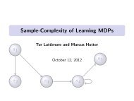
<strong>Online</strong> <strong>Learning</strong> <strong>and</strong> <strong>Game</strong><strong>Theory</strong>+On <strong>Learning</strong> withSimilarity FunctionsYour Guide:Avrim BlumCarnegie Mellon University[Machine <strong>Learning</strong> Summer School 20<strong>08</strong>]
Plan for the tour: Stop 1: <strong>Online</strong> learning, minimizing regret,<strong>and</strong> combining expert advice. Stop 2: <strong>Game</strong> theory, minimax optimality,<strong>and</strong> Nash equilibria. Stop 3: Correlated equilibria, internalregret, routing games, <strong>and</strong> connectionsbetween 1 <strong>and</strong> 2. Stop 4: (something completely different)<strong>Learning</strong> <strong>and</strong> clustering with similarityfunctions.
Some books/references: Algorithmic <strong>Game</strong> <strong>Theory</strong>, Nisan, Roughgarden,Tardos, Vazirani (eds), Cambridge Univ Press, 2007.[Chapter 4 “<strong>Learning</strong>, <strong>Regret</strong> <strong>Minimization</strong>, & Equilibria”is on my webpage] Prediction, <strong>Learning</strong>, & <strong>Game</strong>s, Cesa-Bianchi &Lugosi, Cambridge Univ Press, 2006. My course notes: www.machinelearning.com Stop 1: <strong>Online</strong> learning, minimizing regret, <strong>and</strong> combiningexpert advice. Stop 2: <strong>Game</strong> theory, minimax optimality, <strong>and</strong> Nashequilibria. Stop 3: Correlated equilibria, internal regret, routinggames, <strong>and</strong> connections between 1 <strong>and</strong> 2. Stop 4: (something completely different) <strong>Learning</strong> <strong>and</strong>clustering with similarity functions.
Stop 1: <strong>Online</strong> learning,minimizing regret, <strong>and</strong>combining expert advice
Consider the following setting… Each morning, you need to pickone of N possible routes to driveto work. But traffic is different each day.Not clear a priori which will be best.When you get there you find out howlong your route took. (And maybeothers too or maybe not.) Is there a strategy for picking routes so that in thelong run, whatever the sequence of traffic patternshas been, you’ve done nearly as well as the best fixedroute in hindsight? (In expectation, over internalr<strong>and</strong>omness in the algorithm) Yes.CMU32 min
“No-regret” algorithms for repeated decisionsA bit more generally: Algorithm has N options. World chooses cost vector.Can view as matrix like this (maybe infinite # cols)World – life - fateAlgorithm At each time step, algorithm picks row, life picks column.Alg pays cost for action chosen.Alg gets column as feedback (or just its own cost inthe “b<strong>and</strong>it” model).Need to assume some bound on max cost. Let’s say allcosts between 0 <strong>and</strong> 1.
“No-regret” algorithms for repeated decisions At each time step, algorithm picks row, life picks column.Define Algaverage pays cost regret for action in T time chosen. steps as:(avg per-day cost of alg) – (avg per-day cost of best Alg gets column as feedback (or just its own cost infixed row in hindsight).the “b<strong>and</strong>it” model).We want this to go to 0 or better as T gets large.[called Need a “no-regret” to assume some algorithm] bound on max cost. Let’s say allcosts between 0 <strong>and</strong> 1.
Some intuition & properties of no-regret algs. Let’s s look at a small example:dest Note: Not trying to compete with bestadaptive strategy – just best fixedpath in hindsight. No-regret algorithms can do muchbetter than playing minimax optimal,<strong>and</strong> never much worse. Existence of no-regretalgs yieldsimmediate proof of minimax thm!AlgorithmWorld – life - fate1 00 1Will define thislaterThis too
Some intuition & properties of no-regret algs. Let’s s look at a small example:destAlgorithmWorld – life - fate1 00 1 View of world/life/fate: unknown sequence LRLLRLRR... Goal: do well (in expectation) no matter what thesequence is. Algorithms must be r<strong>and</strong>omized or else it’s s hopeless. Viewing as game: algorithm against the world.
History <strong>and</strong> development (abridged) [Hannan’57, Blackwell’56]: Alg. with regret O((N/T) 1/2 ). Re-phrasing, need only T = O(N/ε 2 ) steps to get time-average regret down to ε. (will call this quantity T ε ) Optimal dependence on T (or ε). . <strong>Game</strong>-theoristsviewed #rows N as constant, not so important as T, sopretty much done.Why optimal in T?dest•Say world flips fair coin each day.•Any alg, in T days, has expected cost T/2.•But E[min(# heads,#tails)] = T/2 – O(T 1/2 ).•So, per-day gap is O(1/T 1/2 ).AlgorithmWorld – life - fate1 00 1
History <strong>and</strong> development (abridged) [Hannan’57, Blackwell’56]: Alg. with regret O((N/T) 1/2 ). Re-phrasing, need only T = O(N/ε 2 ) steps to get time-average regret down to ε. (will call this quantity T ε ) Optimal dependence on T (or ε). . <strong>Game</strong>-theoristsviewed #rows N as constant, not so important as T, sopretty much done. <strong>Learning</strong>-theory 80s-90s:“combining expert advice”.Imagine large class C of N prediction rules. Perform (nearly) as well as best f2C. f [LittlestoneittlestoneWarmuth’89]: Weighted-majority algorithmE[cost] · OPT(1+ε) ) + (log N)/ε.<strong>Regret</strong> O((log N)/T) 1/2 . T ε= O((log N)/ε 2 ). Optimal as fn of N too, plus lots of work on exactconstants, 2 nd order terms, etc. [CFHHSW93]… Extensions to b<strong>and</strong>it model (adds extra factor of N).
To think about this, let’s look atthe problem of “combining expertadvice”.
Using “expert” adviceSay we want to predict the stock market.• We solicit N “experts” for their advice. (Willthe market go up or down?)• We then want to use their advice somehow tomake our prediction. E.g.,Can we do nearly as well as best in hindsight?[“expert” ´ someone with an opinion. Not necessarily someonewho knows anything.]
• We have N “experts”.Simpler question• One of these is perfect (never makes a mistake).We just don’t know which one.• Can we find a strategy that makes no more thanlg(N) mistakes?Answer: sure. Just take majority vote over allexperts that have been correct so far.Each mistake cuts # available by factor of 2.Note: this means ok for N to be very large.“halving algorithm”
Using “expert” adviceBut what if none is perfect? Can we donearly as well as the best one in hindsight?Strategy #1:• Iterated halving algorithm. Same as before, butonce we've crossed off all the experts, restartfrom the beginning.• Makes at most lg(N)[OPT+1] mistakes, where OPTis #mistakes of the best expert in hindsight.Seems wasteful. Constantly forgetting what we've“learned”. Can we do better?
Weighted Majority AlgorithmIntuition: Making a mistake doesn't completelydisqualify an expert. So, instead of crossingoff, just lower its weight.Weighted Majority Alg:– Start with all experts having weight 1.– Predict based on weighted majority vote.– Penalize mistakes by cutting weight in half.
Analysis: do nearly as well as bestexpert in hindsight• M = # mistakes we've made so far.• m = # mistakes best expert has made so far.• W = total weight (starts at N).• After each mistake, W drops by at least 25%.So, after M mistakes, W is at most N(3/4) M .• Weight of best expert is (1/2) m . So,constantratio
R<strong>and</strong>omized Weighted Majority2.4(m + lg N) not so good if the best expert makes amistake 20% of the time. Can we do better? Yes.• Instead of taking majority vote, use weights asprobabilities. (e.g., if 70% on up, 30% on down, then pick70:30) Idea: smooth out the worst case.• Also, generalize ½ to 1- ε.M = expected#mistakesunlike mostworst-casebounds, numbersare pretty good.
Analysis• Say at time t we have fraction F t of weight onexperts that made mistake.• So, we have probability F t of making a mistake, <strong>and</strong>we remove an εF t fraction of the total weight.– W final = N(1-ε F 1 )(1 - ε F 2 )...– ln(W final ) = ln(N) + ∑ t [ln(1 - ε F t )] · ln(N) - ε ∑ t F t(using ln(1-x) < -x)= ln(N) - ε M. (∑ F t = E[# mistakes])• If best expert makes m mistakes, then ln(W final ) > ln((1-ε) m ).• Now solve: ln(N) - ε M > m ln(1-ε).
Summarizing• E[# mistakes] · (1+ε)m + ε -1 log(N).• If set ε=(log(N)/m) 1/2 to balance the twoterms out (or use guess-<strong>and</strong>-double), getbound of E[mistakes]·m+2(m¢log N) 1/2• Since m · T, this is at most m + 2(Tlog N) 1/2 .• So, regret ! 0.
What if we have N options,not N predictors?• We’re not combining N experts, we’rechoosing one. Can we still do it?• Nice feature of RWM: can still apply.– Choose expert i with probability p i = w i /W.– Still the same algorithm!– Can apply to choosing N options, so long as costsare {0,1}.– What about costs in [0,1]?
What if we have N options,not N predictors?What about costs in [0,1]?• If expert i has cost c i , do: w i à w i (1-c i ε).• Our expected cost = ∑ i c i w i /W.• Amount of weight removed = ε ∑ i w i c i .• So, fraction removed = ε ¢ (our cost).• Rest of proof continues as before…• So, now we can drive to work! (assuming fullfeedback)
Efficient implicit implementation for large N… Bounds have only log dependence on # choices N. So, conceivably can do well when N is exponentialin natural problem size, if only could implementefficiently. E.g., case of paths…dest nxn grid has N = (2n choose n) possible paths. Recent years: series of results giving efficientimplementation/alternatives in various settings,plus extensions to b<strong>and</strong>it model.
Efficient implicit implementation for large N… Recent years: series of results giving efficientimplementation/alternatives in various settings: [HelmboldelmboldSchapire97]:best pruning of given DT. [BChawlahawlaKalai02]:list-update problem. [TakimotoakimotoWarmuth02]:online shortest path in DAGs. [KalaialaiVempala03]:elegant setting generalizing all above <strong>Online</strong> linear programming [Zinkevichinkevich03]:elegant setting generalizing all above <strong>Online</strong> convex programming [AwerbuchwerbuchKleinberg04][McMahanB04]:B04]:[KV] [KV]!b<strong>and</strong>it model [Kleinbergleinberg,FlaxmanKalaiMcMahan05]:[Z03] ! b<strong>and</strong>it model [DanianiHayes06]:improve b<strong>and</strong>it convergence rateMore…
[Kalai-Vempala’03] <strong>and</strong> [Zinkevich’03] settings[KV] setting: Implicit set S of feasible points in R m . (E.g., m=#edges,S={indicator vectors 011010010 for possible paths}) Assume have oracle for offline problem: given vector c,find x 2 S to minimize c¢x. (E.g., shortest pathalgorithm) Use to solve online problem: on day t, , must pick x 2 Sbefore c is given. (c [Z] setting:1 ¢x 1 +…+c T ¢x T )/T ! min x2S x¢(c1 +…+c T )/T.x Assume S is convex. Allow c(x) to be a convex function over S. Assume given any y not in S, can algorithmically findnearest x 2 S.
Problems that can be modeled:<strong>Online</strong> shortest paths.Web-searchsearch-results results ordering problem: For a given query (say, “Ancient Greece”), output anordering of search results based on what people haveclicked on before, where cost = f(depth of item clicked)(S = set of permutation matrices)Some inventory problems, adaptive pricingproblems
Kalai-Vempala algorithm Recall setup: Set S of feasible points in R m , ofbounded diameter. For = 1 to T: Alg picks x 2 S, adversary pickscost vector c , Alg pays x ¢ c . Goal: compete withx 2 S that minimizes ⌧ ¢ (c 1 + c 2 + … + c T ). Assume have oracle for offline problem:xgiven c, find best x 2 S. Use to solve online. Algorithm is very simple: Just pick x 2 S that minimizes x¢(c 0 + c 1 + … + c -1 ),where c 0 is picked from appropriate distribution.(in fact, closely related to Hannan’s original alg.) Form of bounds: T ε = O(diam(S) ¢ L 1 bound on c’s ¢ log(m)/ ε 2 ). For online shortest path, T ε = O(nm¢log(n)/ε 2 ).
Analysis sketch [KV]Two algorithms walk into a bar… Alg A picks x minimizing x ¢c -1 , where c -1 =c 1 +…+c -1 . Alg B picks x minimizing x ¢c , where c =c 1 +…+c .(B has fairy godparents who add c into history)Step 1: prove B is at least as good as OPT:∑ t (B’s x t )¢ c t · min x2 S x¢(c 1 + … + c T )Uses cute telescoping argument.Now, A & B start drinking <strong>and</strong> their objectives get fuzzier…Step 2: at appropriate point (width ofdistribution for c 0 ), prove A & B aresimilar <strong>and</strong> yet B has not been hurt toomuch.C t-1 C t
B<strong>and</strong>it setting What if alg is only told cost ⌧ ¢♍ <strong>and</strong> not ♍ itself. E.g., you only find out cost of your own path, not alledges in network. Can you still perform comparably to the best path inhindsight? (which you don’t even know!) Ans: yes, though bounds are worse. Basic idea is fairlystraightforward: All we need is an estimate of c t-1 =c 1 + … + c t-1 . So, pick basis B <strong>and</strong> occasionally sample a r<strong>and</strong>om x2B. Use dot-products with basis vectors to reconstructestimate of c t-1 . (Helps for B to be as orthogonal aspossible) Even if world is adaptive (knows what you know), stillcan’t bias your estimate too much if you do it right.
A natural generalization A natural generalization of our regret goal is: what if wealso want that on rainy days, we do nearly as well as thebest route for rainy days. And on Mondays, do nearly as well as best route forMondays. More generally, have N “rules” (on Monday, use path P).Goal: simultaneously, for each rule i, guarantee to donearly as well as it on the time steps in which it fires. For all i, want E[cost i (alg)] · (1+ε)cost i (i) + O(ε -1 log N).(cost i (X) = cost of X on time steps where rule i fires.) Can we get this?
A natural generalization This generalization is esp natural in machine learning forcombining multiple if-then rules. E.g., document classification. Rule: “if appearsthen predict ”. E.g., if has football then classify assports. So, if 90% of documents with football are about sports,we should have error · 11% on them.“Specialists” or “sleeping experts” problem.Studied theoretically in [B95][FSSW97][BM05];experimentally [CS’96,CS’99]. Assume we have N rules, explicitly given. For all i, want E[cost i (alg)] · (1+ε)cost i (i) + O(ε -1 log N).(cost i (X) = cost of X on time steps where rule i fires.)
A simple algorithm <strong>and</strong> analysis (all on one slide) Start with all rules at weight 1. At each time step, of the rules i that fire,select one with probability p i / wi. Update weights:If didn’t fire, leave weight alone.If did fire, raise or lower depending on performancecompared to weighted average:r i= [∑ jp jcost(j)]/(1+ε) – cost(i)w ià w i(1+ε) r iSo, if rule i does exactly as well as weighted average,its weight drops a little. Weight increases if doesbetter than weighted average by more than a (1+ε)factor. This ensures sum of weights doesn’t increase. Final w i = (1+ε) E[cost i(alg)]/(1+ε)-costi(i). So, exponent · ε -1 log N. So, E[cost i (alg)] · (1+ε)cost i (i) + O(ε -1 log N).
Can combine with [KV],[Z] too: Back to driving, say we are given N “conditions” to payattention to (is it raining?, is it a Monday?, …). Each day satisfies some <strong>and</strong> not others. Wantsimultaneously for each condition (incl default) to donearly as well as best path for those days. To solve, create N rules: “if day satisfies condition i,then use output of KV i ”, where KV i is an instantiation ofKV algorithm you run on just the days satisfying thatcondition.
Stop 2: <strong>Game</strong> <strong>Theory</strong>
Consider the following scenario…• Shooter has a penalty shot. Can choose toshoot left or shoot right.• Goalie can choose to dive left or dive right.• If goalie guesses correctly, (s)he saves theday. If not, it’s a goooooaaaaall!• Vice-versa for shooter.
2-Player Zero-Sum games• Two players R <strong>and</strong> C. Zero-sum means that what’sgood for one is bad for the other.• <strong>Game</strong> defined by matrix with a row for each of R’soptions <strong>and</strong> a column for each of C’s options.Matrix tells who wins how much.• an entry (x,y) means: x = payoff to row player, y = payoff tocolumn player. “Zero sum” means that y = -x.• E.g., penalty shot:Left RightgoalieshooterLeft(0,0) (1,-1)GOAALLL!!!Right(1,-1) (0,0)No goal
<strong>Game</strong> <strong>Theory</strong> terminolgy• Rows <strong>and</strong> columns are called pure strategies.• R<strong>and</strong>omized algs called mixed strategies.• “Zero sum” means that game is purelycompetitive. (x,y) satisfies x+y=0. (<strong>Game</strong>doesn’t have to be fair).Left RightgoalieshooterLeft(0,0) (1,-1)GOAALLL!!!Right(1,-1) (0,0)No goal
Minimax-optimal strategies• Minimax optimal strategy is a (r<strong>and</strong>omized)strategy that has the best guarantee on itsexpected gain, over choices of the opponent.[maximizes the minimum]• I.e., the thing to play if your opponent knowsyou well.Left RightgoalieshooterLeft(0,0) (1,-1)GOAALLL!!!Right(1,-1) (0,0)No goal
Minimax-optimal strategies• Can solve for minimax-optimal strategiesusing Linear programming• I.e., the thing to play if your opponent knowsyou well.Left RightgoalieshooterLeft(0,0) (1,-1)GOAALLL!!!Right(1,-1) (0,0)No goal
Minimax-optimal strategies• What are the minimax optimal strategies forthis game?Minimax optimal strategy for both players is50/50. Gives expected gain of ½ for shooter(-½ for goalie). Any other is worse.Left RightgoalieshooterLeft(0,0) (1,-1)GOAALLL!!!Right(1,-1) (0,0)No goal
Minimax-optimal strategies• How about penalty shot with goalie who’sweaker on the left?Minimax optimal for shooter is (2/3,1/3).Guarantees expected gain at least 2/3.Minimax optimal for goalie is also (2/3,1/3).Guarantees expected loss at most 2/3.Left RightgoalieshooterLeft(½,-½) (1,-1)GOAALLL!!!Right(1,-1) (0,0)50/50
Shall we play a game...?I put either a quarter or nickelin my h<strong>and</strong>. You guess. If youguess right, you get the coin.Else you get nothing.All right!
Summary of gameValue to guesserguess: NQhideN Q5 00 25Should guesser always guess Q? 50/50?What is minimax optimal strategy?
Summary of gameValue to guesserguess: NQhideN Q5 00 25If guesser always guesses Q, then hider willhide N. Value to guesser = 0.If guesser does 50/50, hider will still hide N.E[value to guesser] = ½(5) + ½(0) = 2.5
Summary of gameValue to guesserguess: NQhideN Q5 00 25If guesser guesses 5/6 N, 1/6 Q, then:• if hider hides N, E[value] = (5/6)*5 ~ 4.2• if hider hides Q, E[value] = 25/6 also.
Summary of gameValue to guesserguess: NQhideN Q5 00 25What about hider?Minimax optimal strategy: 5/6 N, 1/6 Q.Guarantees expected loss at most 25/6, nomatter what the guesser does.
Interesting. The hider has a(r<strong>and</strong>omized) strategy he canreveal with expected loss · 4.2against any opponent, <strong>and</strong> theguesser has a strategy she canreveal with expected gain ¸ 4.2against any opponent.
Minimax Theorem (von Neumann 1928)• Every 2-player zero-sum game has a uniquevalue V.• Minimax optimal strategy for R guaranteesR’s expected gain at least V.• Minimax optimal strategy for C guaranteesC’s expected loss at most V.Counterintuitive: Means it doesn’t hurt topublish your strategy if both players areoptimal. (Borel had proved for symmetric 5x5but thought was false for larger games)
Nice proof of minimax thm• Suppose for contradiction it was false.• This means some game G has V C > V R :– If Column player commits first, there existsa row that gets the Row player at least V C .– But if Row player has to commit first, theColumn player can make him get only V R .• Scale matrix so payoffs to row arein [-1,0]. Say V R = V C - δ.V CV R
Proof contd• Now, consider playing r<strong>and</strong>omized weightedmajorityalg as Row, against Col who playsoptimally against Row’s distrib.• In T steps,– Alg gets ¸ (1−ε/2)[best row in hindsight] – log(N)/ε– BRiH ¸ T¢V C [Best against opponent’s empiricaldistribution]– Alg · T¢V R [Each time, opponent knows yourr<strong>and</strong>omized strategy]– Gap is δT. Contradicts assumption if use ε=δ, onceT > 2log(N)/ε 2 .
Can use notion of minimaxoptimality to explain bluffingin poker
Simplified Poker (Kuhn 1950)• Two players A <strong>and</strong> B.• Deck of 3 cards: 1,2,3.• Players ante $1.• Each player gets one card.• A goes first. Can bet $1 or pass.• If A bets, B can call or fold.• If A passes, B can bet $1 or pass.– If B bets, A can call or fold.• High card wins (if no folding). Max pot $2.
• Two players A <strong>and</strong> B. 3 cards: 1,2,3.• Players ante $1. Each player gets one card.• A goes first. Can bet $1 or pass.• If A bets, B can call or fold.• If A passes, B can bet $1 or pass.– If B bets, A can call or fold.Writing as a Matrix <strong>Game</strong>• For a given card, A can decide to• Pass but fold if B bets. [PassFold]• Pass but call if B bets. [PassCall]• Bet. [Bet]• Similar set of choices for B.
[PF,PF,PC][PF,PF,B][PF,PC,PC][PF,PC,B][B,PF,PC][B,PF,B][B,PC,PC][B,PC,B]Can look at all strategies as abig matrix…[FP,FP,CB] [FP,CP,CB] [FB,FP,CB] [FB,CP,CB]0 0 -1/6 -1/60 1/6 -1/3 -1/6-1/6 0 0 1/6-1/6 –1/6 1/6 1/6-1/6 0 0 1/61/6 –1/3 0 –1/21/6 –1/6 –1/6 –1/20 –1/2 1/3 –1/60 –1/3 1/6 –1/6
And the minimax optimalstrategies are…• A:– If hold 1, then 5/6 PassFold <strong>and</strong> 1/6 Bet.– If hold 2, then ½ PassFold <strong>and</strong> ½ PassCall.– If hold 3, then ½ PassCall <strong>and</strong> ½ Bet.Has both bluffing <strong>and</strong> underbidding…• B:– If hold 1, then 2/3 FoldPass <strong>and</strong> 1/3 FoldBet.– If hold 2, then 2/3 FoldPass <strong>and</strong> 1/3 CallPass.– If hold 3, then CallBetMinimax value of game is –1/18 to A.
Recent work• [Gilpin & S<strong>and</strong>holm] solved for minimaxoptimal in micro version of 2-player Texashold’em (Rhode Isl<strong>and</strong> hold’em).[52 card deck. Ante of $5. Get one card facedown. Round of betting at $10. Flop card. Roundof betting at $20. Turn card. Round of bettingat $20. Showdown with 3-card h<strong>and</strong>s.]– Use various methods to reduce to LP with about1m rows/cols. Solving: 1 week using 25 gig RAM.• [McMahan & Gordon] show online learningtechniques can get minimax 2[-0.28,-0.46] in2 hrs.
Now, to General-Sum games!
General-Sum <strong>Game</strong>s• Zero-sum games are good formalism forworst-case analysis of algorithms.• General-sum games are good models forsystems with many participants whosebehavior affects each other’s interests– E.g., routing on the internet– E.g., online auctions
General-sum games• In general-sum games, can get win-win<strong>and</strong> lose-lose situations.• E.g., “what side of sidewalk to walk on?”:youLeftLeft Right(1,1) (-1,-1)personwalkingtowards youRight(-1,-1) (1,1)
General-sum games• In general-sum games, can get win-win<strong>and</strong> lose-lose situations.• E.g., “which movie should we go to?”:Spartans AtonementSpartans(8,2) (0,0)Atonement(0,0) (2,8)No longer a unique “value” to the game.
Nash Equilibrium• A Nash Equilibrium is a stable pair ofstrategies (could be r<strong>and</strong>omized).• Stable means that neither player hasincentive to deviate on their own.• E.g., “what side of sidewalk to walk on”:Left RightLeftRight(1,1) (-1,-1)(-1,-1) (1,1)NE are: both left, both right, or both 50/50.
Nash Equilibrium• A Nash Equilibrium is a stable pair ofstrategies (could be r<strong>and</strong>omized).• Stable means that neither player hasincentive to deviate on their own.• E.g., “which movie to go to”:Spartans AtonementSpartansAtonement(8,2) (0,0)(0,0) (2,8)NE are: both S, both A, or (80/20,20/80)
Uses• Economists use games <strong>and</strong> equilibria asmodels of interaction.• E.g., pollution / prisoner’s dilemma:– (imagine pollution controls cost $4 but improveeveryone’s environment by $3)don’t pollute pollutedon’t pollutepollute(2,2) (-1,3)(3,-1) (0,0)Need to add extra incentives to get good overall behavior.
NE can do strange things• Braess paradox:– Road network, traffic going from s to t.– travel time as function of fraction x oftraffic on a given edge.travel time = 1,indep of traffics1xtravel timet(x)=x.tx1Fine. NE is 50/50. Travel time = 1.5
NE can do strange things• Braess paradox:– Road network, traffic going from s to t.– travel time as function of fraction x oftraffic on a given edge.travel time = 1,indep of trafficsx10x1travel timet(x)=x.tAdd new superhighway. NE: everyoneuses zig-zag path. Travel time = 2.
Existence of NE• Nash (1950) proved: any general-sum gamemust have at least one such equilibrium.– Might require r<strong>and</strong>omized strategies (called“mixed strategies”)• This also yields minimax thm as a corollary.– Pick some NE <strong>and</strong> let V = value to row player inthat equilibrium.– Since it’s a NE, neither player can do bettereven knowing the (r<strong>and</strong>omized) strategy theiropponent is playing.– So, they’re each playing minimax optimal.
Existence of NE• Proof will be non-constructive.• Unlike case of zero-sum games, we do notknow any polynomial-time algorithm forfinding Nash Equilibria in n £ n general-sumgames. [known to be “PPAD-hard”]• Notation:– Assume an nxn matrix.– Use (p 1 ,...,p n ) to denote mixed strategy for rowplayer, <strong>and</strong> (q 1 ,...,q n ) to denote mixed strategyfor column player.
Proof• We’ll start with Brouwer’s fixed pointtheorem.– Let S be a compact convex region in R n <strong>and</strong> letf:S ! S be a continuous function.– Then there must exist x 2 S such that f(x)=x.– x is called a “fixed point” of f.• Simple case: S is the interval [0,1].• We will care about:– S = {(p,q): p,q are legal probability distributionson 1,...,n}. I.e., S = simplex n £ simplex n
Proof (cont)• S = {(p,q): p,q are mixed strategies}.• Want to define f(p,q) = (p’,q’) such that:– f is continuous. This means that changing por q a little bit shouldn’t cause p’ or q’ tochange a lot.– Any fixed point of f is a Nash Equilibrium.• Then Brouwer will imply existence of NE.
Try #1• What about f(p,q) = (p’,q’) where p’ is bestresponse to q, <strong>and</strong> q’ is best response to p?• Problem: not necessarily well-defined:– E.g., penalty shot: if p = (0.5,0.5) then q’ couldbe anything.Left RightLeftRight(0,0) (1,-1)(1,-1) (0,0)
Try #1• What about f(p,q) = (p’,q’) where p’ is bestresponse to q, <strong>and</strong> q’ is best response to p?• Problem: also not continuous:– E.g., if p = (0.51, 0.49) then q’ = (1,0). If p =(0.49,0.51) then q’ = (0,1).Left RightLeftRight(0,0) (1,-1)(1,-1) (0,0)
Instead we will use...• f(p,q) = (p’,q’) such that:– q’ maximizes [(expected gain wrt p) - ||q-q’|| 2 ]– p’ maximizes [(expected gain wrt q) - ||p-p’|| 2 ]p p’Note: quadratic + linear = quadratic.
Instead we will use...• f(p,q) = (p’,q’) such that:– q’ maximizes [(expected gain wrt p) - ||q-q’|| 2 ]– p’ maximizes [(expected gain wrt q) - ||p-p’|| 2 ]p’ pNote: quadratic + linear = quadratic.
Instead we will use...• f(p,q) = (p’,q’) such that:– q’ maximizes [(expected gain wrt p) - ||q-q’|| 2 ]– p’ maximizes [(expected gain wrt q) - ||p-p’|| 2 ]• f is well-defined <strong>and</strong> continuous sincequadratic has unique maximum <strong>and</strong> smallchange to p,q only moves this a little.• Also fixed point = NE. (even if tinyincentive to move, will move little bit).• So, that’s it!
One more interesting game“Ultimatum game”:• Two players “Splitter” <strong>and</strong> “Chooser”• 3 rd party puts $10 on table.• Splitter gets to decide how to splitbetween himself <strong>and</strong> Chooser.• Chooser can accept or reject.• If reject, money is burned.
One more interesting game“Ultimatum game”: E.g., with $4Chooser:howmuch toaccept123Splitter: how muchto offer chooser1 2 3(1,3) (2,2) (3,1)(0,0) (2,2) (3,1)(0,0) (0,0) (3,1)
Boosting & game theory• Suppose I have an algorithm A that for anydistribution (weighting fn) over a dataset Scan produce a rule h2H that gets < 40%error.• Adaboost gives a way to use such an A toget error ! 0 at a good rate, using weightedvotes of rules produced.• How can we see that this is even possible?
Boosting & game theory• Assume for all D over cols,exists a row with cost < 0.4.• Minimax implies must exist aweighting over rows s.t. forevery x i , the vote is at least60/40 in the right way.• So, weighted vote has L 1margin at least 0.2.• (Of course, AdaBoost givesyou a way to get at it withonly access via A. But this atleast implies existence…)h 1h 2…h mx 1 , x 2 , x 3 ,…, x nEntry ij = 1 ifh i (x j ) isincorrect, 0if correct
Stop 3: What happens ifeveryone is adaptingtheir behavior?
What if everyone started using no-regret algs? What if changing cost function is due to otherplayers in the system optimizing for themselves? No-regret can be viewed as a nice definition ofreasonable self-interested behavior. So, whathappens to overall system if everyone uses one? In zero-sum games, empirical frequencies quicklyapproaches minimax optimal. If your empirical distribution of play didn’t,then opponent would be able to (<strong>and</strong> have to)take advantage, giving you < V.
What if everyone started using no-regret algs? What if changing cost function is due to otherplayers in the system optimizing for themselves? No-regret can be viewed as a nice definition ofreasonable self-interested behavior. So, whathappens to overall system if everyone uses one? In zero-sum games, empirical frequencies quicklyapproaches minimax optimal. In general-sum games, does behavior quickly (orat all) approach a Nash equilibrium? (after all, aNash Eq is exactly a set of distributions thatare no-regretwrt each other). Well, unfortunately, no.
A bad example for general-sum games Augmented Shapley game from [Z04]: “RPSF” First 3 rows/cols are Shapley game (rock / paper /scissors but if both do same action then both lose). 4 th action “play foosball” has slight negative if otherplayer is still doing r/p/s but positive if other playerdoes 4 th action too. NR algs will cycle among first 3 <strong>and</strong> have no regret,but do worse than only Nash Equilibrium of bothplaying foosball. We didn’t t really expect this to work given howhard NE can be to find…
What can we say? If algorithms minimize “internal” or “swap”regret, then empirical distribution of playapproaches correlated equilibrium.Foster & Vohra, Hart & Mas-Colell,…Though doesn’t imply play is stabilizing. In some natural cases, like routing in Wardropmodel, , can show daily traffic actually approachesNash.
More general forms of regret1. “best expert” or “external” regret:– Given n strategies. Compete with best of them inhindsight.2. “sleeping expert” or “regret with time-intervals”:– Given n strategies, k properties. Let S i be set of dayssatisfying property i (might overlap). Want tosimultaneously achieve low regret over each S i .3. “internal” or “swap” regret: like (2), except thatS i = set of days in which we chose strategy i.
Internal/swap-regretregret• E.g., each day we pick one stock to buyshares in.– Don’t want to have regret of the form “everytime I bought IBM, I should have boughtMicrosoft instead”.• Formally, regret is wrt optimal functionf:{1,…,N}!{1,…,N} such that every time youplayed action j, it plays f(j).• Motivation: connection to correlatedequilibria.
Internal/swap-regretregret“Correlated equilibrium”– Distribution over entries in matrix, such that ifa trusted party chooses one at r<strong>and</strong>om <strong>and</strong> tellsyou your part, you have no incentive to deviate.– E.g., Shapley game.R P SRPS-1,-1 -1,1 1,-11,-1 -1,-1 -1,1-1,1 1,-1 -1,-1
Internal/swap-regretregret• If all parties run a low internal/swap regretalgorithm, then empirical distribution ofplay is an apx correlated equilibrium.– Correlator chooses r<strong>and</strong>om time t 2 {1,2,…,T}.Tells each player to play the action j theyplayed in time t (but does not reveal value of t).– Expected incentive to deviate:∑ j Pr(j)(<strong>Regret</strong>|j)= swap-regret of algorithm– So, this says that correlated equilibria are anatural thing to see in multi-agent systemswhere individuals are optimizing for themselves
Internal/swap-regret,regret, contdAlgorithms for achieving low regret of thisform:– Foster & Vohra, Hart & Mas-Colell, Fudenberg& Levine.– Can also convert any “best expert” algorithminto one achieving low swap regret.– Unfortunately, time to achieve low regret islinear in n rather than log(n)….
Internal/swap-regret,regret, contdCan convert any “best expert” algorithm A into oneachieving low swap regret. Idea:– Instantiate one copy A i responsible forexpected regret over times we play i.– Each time step, if we play p=(p 1 ,…,p n ) <strong>and</strong> getcost vector c=(c 1 ,…,c n ), then A i gets cost-vectorp i c.– If each A i proposed to play q i , so all togetherwe have matrix Q, then define p = pQ.– Allows us to view p i as prob we chose action i orprob we chose algorithm A i .
What can we say? If algorithms minimize “internal” or “swap”regret, then empirical distribution of playapproaches correlated equilibrium.Foster & Vohra, Hart & Mas-Colell,…Though doesn’t imply play is stabilizing. In some natural cases, like routing in Wardropmodel, , can show daily traffic actually approachesNash.
Consider Wardrop/Roughgarden-Tardos traffic model Given a graph G. Each edge e has non-decreasing costfunction c e (f e ) that tells latency of that edge as afunction of the amount of traffic using it. Say 1 unit of traffic (infinitesimal users) wants to travelfrom v s to v t . E.g., simple case: Nash equilibrium is flow f*such that all paths withpositive flow have the samecost, <strong>and</strong> no path is cheaper. c e(f)=fNash is 2/3,1/3c e(f)=2f Cost(f) = ∑ e c e (f e )f e = cost of average user under f. Cost f (P) = ∑ e 2 P c e (f e ) = cost of using path P given f.So, at Nash, Cost(f*) = min P Cost f* (P). What happens if people use no-regret algorithms?
Consider Wardrop/Roughgarden-Tardos traffic model These are “potential games” so Nash Equilibriaare not that hard to find. In fact, a number of distributed procedures areknown that will approach Nash at a good rate.Analyzing result of no-regret algorithms ¼ areNash Equilibria the inevitable result of usersintelligently behaving in their own interest?
Global behavior of NR algs Interesting case to consider: 2/31/3 NR alg: cost approaches ½ per day, which iscost of best fixed path in hindsight.But none of the individual days is an ε-Nashflow (a flow where only a small fraction oftraffic has significant incentive to switch).Same for time-average flow f avg .
Global behavior of NR algs [B-EvenDar-Ligett]Assuming edge latency functions have boundedslope, can show that traffic flow approachesequilibrium in that for ε!0 we have: For 1-ε fraction of days, a 1-ε fraction of peoplehave at most ε incentive to deviate. (traveling ona path at most ε worse than optimal given thetraffic flow). And you really do need all three caveats. E.g., ifusers are running b<strong>and</strong>it algorithms, then on anygiven day a small fraction will be performing“exploration” steps.
Global behavior of NR algs [B-EvenDar-Ligett]Argument outline:1. For any edge e, , time-avgcost · flow-avgcost. So,avg t [c e (f )] · avg [c e (f ) ¢ f ]/ f avge
Global behavior of NR algs [B-EvenDar-Ligett]Argument outline:1. For any edge e, , time-avgcost · flow-avgcost. So,f avg e ¢ avg t [c e (f )] · avg [c e (f ) ¢ f ]2. Summing over all edges, <strong>and</strong> applying the regret bound:avg [Cost f (favg )] · avg [Cost(f )] ·ε+minP avg [Cost f (P)],which in turn is · ε +avg [Cost f (favg )].3. This means that actually, for each edge, the time-avgcost must be pretty close to the flow-avgcost, which(by the assumption of bounded slope) means the costscan’t t vary too much over time.4. Once you show costs are stabilizing, then easy to showthat low regret ) Nash conditions approximatelysatisfied.
Global behavior of NR algs [B-EvenDar-Ligett]Argument outline:1. For any edge e, , time-avgcost · flow-avgcost. So,f avg e ¢ avg t [c e (f )] · avg [c e (f ) ¢ f ]2. But can show the sum over all edges of this gap is alower bound on the average regret of the players.3. This means that actually, for each edge, the time-avgcost must be pretty close to the flow-avgcost, which(by the assumption of bounded slope) means the costscan’t t vary too much over time.4. Once you show costs are stabilizing, then easy to showthat low regret ) Nash conditions approximatelysatisfied.
Last stop: On a <strong>Theory</strong> ofSimilarity Functions for<strong>Learning</strong> <strong>and</strong> Clustering[Includes work joint with Nina Balcan,Nati Srebro, <strong>and</strong> Santosh Vempala]
Last stop: On a <strong>Theory</strong> ofSimilarity Functions for<strong>Learning</strong> <strong>and</strong> Clustering[Includes work joint with Nina Balcan,Nati Srebro, <strong>and</strong> Santosh Vempala]
2-minute version• Suppose we are given a set of images , <strong>and</strong>want to learn a rule to distinguish men fromwomen. Problem: pixel representation not so good.• A powerful technique for such settings isto use a kernel: : a special kind of pairwisefunction ( , ).function K( , )• In practice, Caveat:choose speakerK to be good measure ofsimilarity, but theory in terms of implicit mappings.knows next tonothing aboutQ: Can we bridge the gap? <strong>Theory</strong> that just views Kas a measure computer of similarity? vision. Ideally, make it easierto design good functions, & be more general too.
2-minute version• Suppose we are given a set of images , <strong>and</strong>want to learn a rule to distinguish men fromwomen. Problem: pixel representation not so good.• A powerful technique for such settings isto use a kernel: : a special kind of pairwisefunction ( , ).function K( , )• In practice, choose K to be good measure ofsimilarity, but theory in terms of implicit mappings.Q: What if we only have unlabeled data (i.e.,clustering)? Can we develop a theory of propertiesthat are sufficient to be able to cluster well?
2-minute version• Suppose we are given a set of images , <strong>and</strong>want to learn a rule to distinguish men fromwomen. Problem: pixel representation not so good.• A powerful technique for such settings isto use a kernel: : a special kind of pairwisefunction ( , ).function K( , )• In practice, choose K to be good measure ofsimilarity, but theory in terms of implicit mappings.Develop a kind of PAC model for clustering.
Part 1: On similarityfunctions for learning
Kernel functions <strong>and</strong> <strong>Learning</strong>• Back to our generic classification problem.E.g., given a set of images , labeledby gender, learn a rule to distinguish menfrom women. [Goal: do well on new data]• Problem: our best algorithms learn linearseparators, but might not be good fordata in its natural representation.– Old approach: use a more complex class − of+ −functions.– New approach: use a kernel.−++++++ +−− −−−−−−
What’s s a kernel?• A kernel K is a legal def of dot-product: fns.t. there exists an implicit mapping Φ K suchthat K( , )=Φ K ( )¢Φ K ( ).• E.g., K(x,y) = (x ¢ y + 1) d .– Φ K :(n-diml space) ! (n d -diml space).Kernel shouldbe pos. semidefinite(PSD)• Point is: many learning algs can be written soonly interact with data via dot-products.– If replace x¢y with K(x,y), it acts implicitly as ifdata was in higher-dimensional Φ-space.
Example• E.g., for the case of n=2, d=2, the kernelK(x,y) = (1 + x¢y) d corresponds to the mapping:x 2x 1z 2z 1XXXXXXOXXOOXXXOO OO OXXXXXXXz 3OXOOO O OOOOXXXXXXXXXXXX XXX XX
Moreover, generalize well if good margin• If data is lin. separable bymargin γ in Φ-space, then needsample size only Õ(1/γ 2 ) to getconfidence in generalization.Assume |Φ(x)|· 1.• Kernels found to be useful in practice fordealing with many, many different kinds ofdata.-γ γ----+++ + + +
Moreover, generalize well if good margin…but there’s something a little funny:• On the one h<strong>and</strong>, operationally a kernel isjust a similarity measure: K(x,y) 2 [-1,1],with some extra reqts.• But <strong>Theory</strong> talks about margins in implicithigh-dimensional Φ-space. K(x,y) =Φ(x)¢Φ(y).xy
I want to use ML to classify proteinstructures <strong>and</strong> I’m trying to decideon a similarity fn to use. Any help?It should be pos. semidefinite, <strong>and</strong>should result in your data having a largemargin separator in implicit high-dimlspace you probably can’t even calculate.
Umm… thanks, I guess.It should be pos. semidefinite, <strong>and</strong>should result in your data having a largemargin separator in implicit high-dimlspace you probably can’t even calculate.
Moreover, generalize well if good margin…but there’s something a little funny:• On the one h<strong>and</strong>, operationally a kernel isjust a similarity function: K(x,y) 2 [-1,1],with some extra reqts.• But <strong>Theory</strong> talks about margins in implicithigh-dimensional Φ-space. K(x,y) =Φ(x)¢Φ(y).– Can we bridge the gap?– St<strong>and</strong>ard theory has a something-for-nothingfeel to it. “All the power of the high-dim’limplicit space without having to pay for it”.More prosaic explanation?xy
Question: do we need thenotion of an implicit space tounderst<strong>and</strong> what makes akernel helpful for learning?
Goal: notion of “good similarity function”for a learning problem that…1. Talks in terms of more intuitive properties (noimplicit high-dimlspaces, no requirement ofpositive-semidefinitenesssemidefiniteness, , etc)E.g., natural properties of weighted graph induced by K.2. If K satisfies these properties for our givenproblem, then has implications to learning3. Is broad: includes usual notion of “good kernel”(one that induces a large margin separator in Φ-space).
Defn satisfying (1) <strong>and</strong> (2):• Say have a learning problem P (distribution Dover examples labeled by unknown target f).• Sim fn K:(x,y)![-1,1] is (ε,γ)-good for P if atleast a 1-ε fraction of examples x satisfy:E y~D [K(x,y)|l(y)=l(x)] ¸ E y~D [K(x,y)|l(y)≠l(x)]+γ“most x are on average more similar to pointsy of their own type than to points y of theother type”
Defn satisfying (1) <strong>and</strong> (2):• Say have a learning problem P (distribution Dover examples labeled by unknown target f).• Sim fn K:(x,y)![-1,1] is (ε,γ)-good for P if atleast a 1-ε fraction of examples x satisfy:E y~D [K(x,y)|l(y)=l(x)] ¸ E y~D [K(x,y)|l(y)≠l(x)]+γ• Note: it’s possible to satisfy this <strong>and</strong> not even bea valid kernel.• E.g., K(x,y) = 0.2 within each class, uniform r<strong>and</strong>omin {-1,1} between classes.
Defn satisfying (1) <strong>and</strong> (2):• Say have a learning problem P (distribution Dover examples labeled by unknown target f).• Sim fn K:(x,y)![-1,1] is (ε,γ)-good for P if atleast a 1-ε fraction of examples x satisfy:E y~D [K(x,y)|l(y)=l(x)] ¸ E y~D [K(x,y)|l(y)≠l(x)]+γHow can we use it?
How to use itAt least a 1-ε prob mass of x satisfy:E y~D [K(x,y)|l(y)=l(x)] ¸ E y~D [K(x,y)|l(y)≠l(x)]+γ• Draw sets S + ,S - of positive/negative points• Classify x based on which gives better score.– Hoeffding: if |S + |,|S - |=O((1/γ 2 )ln 1/δ 2 ), for anygiven “good x”, prob of error over draw of S + ,S −at most δ 2 .– So, at most δ chance our draw is bad on morethan δ fraction of “good x”.• With prob ¸ 1-δ, error rate · ε + δ.
But not broad enough+ +Avg simil to negsis ½, but to pos isonly ½¢1+½¢(-½) =¼._• K(x,y)=x¢y has good separator butdoesn’t satisfy defn. (half of positivesare more similar to negs that to typical pos)
But not broad enough+ +_• Idea: would work if we didn’t pick y’s from top-left.• Broaden to say: OK if 9 large region R s.t. most xare on average more similar to y2R of same labelthan to y2R of other label. (even if don’t know R inadvance)
Broader defn…• Ask that exists a set R of “reasonable” y(allow probabilistic) s.t. almost all x satisfyE y [K(x,y)|l(y)=l(x),R(y)]¸E y [K(x,y)|l(y)≠l(x), R(y)]+γ• And at least ε probability mass ofreasonable positives/negatives.• Claim 1: this is a legitimate way to thinkabout good kernels:– If γ-good kernel then (ε,γ(2 ,ε)-good here.– If γ-good here <strong>and</strong> PSD then γ-good kernel
Broader defn…• Ask that exists a set R of “reasonable” y(allow probabilistic) s.t. almost all x satisfyE y [K(x,y)|l(y)=l(x),R(y)]¸E y [K(x,y)|l(y)≠l(x), R(y)]+γ• And at least ε probability mass ofreasonable positives/negatives.• Claim 2: even if not PSD, can still use forlearning.– So, don’t t need to have implicit-spaceinterpretation to be useful for learning.– But, maybe not with SVMs directly…
How to use such a sim fn?• Ask that exists a set R of “reasonable” y(allow probabilistic) s.t. almost all x satisfyE y [K(x,y)|l(y)=l(x),R(y)]¸E y [K(x,y)|l(y)≠l(x), R(y)]+γ– Draw S = {y 1 ,…,y n }, n¼1/(γ 2 ε). could be unlabeled– View as “l<strong>and</strong>marks”, use to map new data:F(x) = [K(x,y 1 ), …,K(x,y n )].– Whp, exists separator of good L 1 margin inthis space: w=[0,0,1/n + ,1/n + ,0,0,0,-1/n- ,0,0]– So, take new set of examples, project tothis space, <strong>and</strong> run good linear sep. alg.
And furthermoreNow, defn is broad enough to include all largemargin kernels (some loss in parameters):– γ-good margin ) apx (ε,γ 2 ,ε)-good here.But now, we don’t need to think about implicitspaces or require kernel to even have theimplicit space interpretation.If PSD, can also show reverse too:– γ-good here & PSD ) γ-good margin.
And furthermoreIn fact, can even show a separation.• Consider a class C of n pairwise uncorrelatedfunctions over n examples (unif distrib).• Can show that for any kernel K, expectedmargin for r<strong>and</strong>om f in C would be O(1/n 1/2 ).• But, can define a similarity function with γ=1,P(R)=1/n. [K(x i ,x j )=f j (x i )f j (x j )]technically, easier using slight varianton def: E y [K(x,y)l(x)l(y) | R(y)]¸γ
Summary: part 1• Can develop sufficient conditions for asimilarity fn to be useful for learning thatdon’t require notion of implicit spaces.• Property includes usual notion of “goodkernels” modulo the loss in some parameters.– Can apply to similarity fns that aren’t positivesemidefinite(or even symmetric).defn 2defn 1kernel
Summary: part 1• Potentially other interesting sufficientconditions too. E.g., [WangYangFeng07]motivated by boosting.• Ideally, these more intuitive conditions canhelp guide the design of similarity fns for agiven application.
Part 2: Can we use thisangle to help think aboutclustering?
Can we use this angle to help thinkabout clustering?Consider the following setting:• Given data set S of n objects.[documents,web pages]• There is some (unknown) “ground truth” clustering.Each x has true label l(x) in {1,…,t}. [topic]• Goal: produce hypothesis h of low error up toisomorphism of label names.Problem: only have unlabeled data!But, we are given a pairwise similarity fn K.
What conditions on a similarity functionwould be enough to allow one to cluster well?Consider the following setting:• Given data set S of n objects.[documents,web pages]• There is some (unknown) “ground truth” clustering.Each x has true label l(x) in {1,…,t}. [topic]• Goal: produce hypothesis h of low error up toisomorphism of label names.Problem: only have unlabeled data!But, we are given a pairwise similarity fn K.
What conditions on a similarity functionwould be enough to allow one to cluster well?Will lead to something like a PAC model forclustering.Contrast to approx algs approach: view weightedgraph induced by K as ground truth; try tooptimize various objectives.Here, we view target as ground truth. Ask: howshould K be related to let us get at it?
What conditions on a similarity functionwould be enough to allow one to cluster well?Will lead to something like a PAC model forclustering.E.g., say you want alg to cluster docs the way*you* would. How closely related does K haveto be to what’s in your head? Or, given aproperty you think K has, what algs does thatsuggest?
What conditions on a similarity functionwould be enough to allow one to cluster well?Here is a condition that trivially works:Suppose K has property that:• K(x,y) ) > 0 for all x,y such that l(x) ) = l(y).• K(x,y) ) < 0 for all x,y such that l(x) ≠ l(y).If we have such a K, then clustering is easy.Now, let’s try to make this condition a littleweaker….
What conditions on a similarity functionwould be enough to allow one to cluster well?Suppose K has property that all x aremore similar to points y in their owncluster than to any y’ in other clusters.• Still a very strong condition.Problem: the same K can satisfy for two verydifferent clusterings of the same data!baseballMathbasketballPhysics
What conditions on a similarity functionwould be enough to allow one to cluster well?Suppose K has property that all x aremore similar to points y in their owncluster than to any y’ in other clusters.• Still a very strong condition.Problem: the same K can satisfy for two verydifferent clusterings of the same data!baseballbasketballMathPhysicsUnlike learning,you can’t even testyour hypotheses!
Let’s s weaken our goals a bit…• OK to produce a hierarchical clustering(tree) such that correct answer is apxsome pruning of it.baseball– E.g., in case from last slide:all documentssports sciencebaseball basketball math physicsbasketballMathPhysics• We’ll let it be the user’s job to decidehow specific they intended to be.
Then you can start getting somewhere….1.“all x more similar to all y in their own clusterthan to any y’ from any other cluster”is sufficient to get hierarchical clustering such thattarget is some pruning of tree. (Kruskal’s / singlelinkageworks)• Just find most similar pair (x,y) that are indifferent clusters <strong>and</strong> merge their clusterstogether.
Then you can start getting somewhere….1.“all x more similar to all y in their own clusterthan to any y’ from any other cluster”is sufficient to get hierarchical clustering such thattarget is some pruning of tree. (Kruskal’s / singlelinkageworks)2. Weaker condition: ground truth is “stable”:For all clusters C, C’, for all A½C,A’½C’: A <strong>and</strong> A’ are not bothmore similar to each other thanto rest of their own clusters.K(x,y) isattractionbetween x<strong>and</strong> y
Weaker reqt: : correct ans is stableAssume for all C, C’, all A½C, A’µC’, we haveK(A,C-A) > K(A,A’),Avg x2A, y2C-A [K(x,y)]<strong>and</strong> say K is symmetric.Algorithm: average single-linkagelinkage• Like Kruskal, , but at each step merge pair ofclusters whose average similarity is highest.Analysis: (all clusters made are laminar wrt target)• Failure iff merge C 1 , C 2 s.t. C 1 ½C, C 2 ÅC = φ.It’s getting late, let’s skip the proof• But must exist C 3 ½C s.t. K(C 1 ,C 3 ) ¸ K(C 1 ,C-C 1 ), <strong>and</strong>K(C 1 ,C-C 1 ) > K(C 1 ,C 2 ). Contradiction.
Example analysis for simpler versionAssume for all C, C’, all A½C, A’µC’, we haveK(A,C-A) > K(A,A’),[Think of K as “attraction”]Avg x2A, y2C-A [K(x,y)]<strong>and</strong> say K is symmetric.Algorithm breaks down if K is not symmetric:0.250.10.5Instead, run “Boruvka-inspired” algorithm:– Each current cluster C i points to argmax Cj K(C i ,C j )– Merge directed cycles. (not all components)
PropertyStrict SeparationProperties SummaryModel, AlgorithmHierarchical, Linkage basedClusteringComplexityΘ(2 t )Stability, all subsets.(Weak, Strong, etc)Average Attraction(Weighted)Stability of largesubsets (SLS)ν−strict separation(2,ε) k-medianHierarchical, Linkage basedList, Sampling based & NNHierarchical, complexalgorithm (running time t O(t/γ2 ))Hierarchicalspecial case of ν−strictseparation, ν=3εΘ(2 t )t O(t/γ2 )Θ(2 t )Θ(2 t )
PropertyStrict SeparationProperties SummaryModel, AlgorithmHierarchical, Linkage basedClusteringComplexityΘ(2 t )Stability, all subsets.(Weak, Strong, etc)Average Attraction(Weighted)Stability of largesubsets (SLS)ν−strict separation(2,ε) k-medianHierarchical, Linkage basedList, Sampling based & NNHierarchical, complexalgorithm (running time t O(t/γ2 ))Hierarchicalspecial case of ν−strictseparation, ν=3εΘ(2 t )t O(t/γ2 )Θ(2 t )Θ(2 t )
Stability of Large SubsetsFor all C, C’, all A½C, A’µC’, |A|+|A’| ¸ snAlgorithmK(A,C-A) > K(A,A’)+γAA’1) Generate list L of c<strong>and</strong>idate clusters; average attraction alg.Ensure that any ground-truth cluster is f-close to one in L.2) For every pair C, C 0in L that are|C \ C 0| ¸ gn, |C 0\ C| ¸ gn, |C 0Å C| ¸ gnIf K(C Å C 0 , C \ C 0 ) ¸ K(C Å C 0 , C 0 \ C), throw out CElse throw out C 0CC Å C 0C 03) Clean <strong>and</strong> hook up the surviving clusters into a tree
More general conditionsWhat if only require stability for large sets?(Assume all true clusters are large.) E.g, take example satisfyingstability for all sets but add noise. Might cause bottom-up algorithms to fail.Instead, can pick some points at r<strong>and</strong>om,guess their labels, <strong>and</strong> use to cluster therest. Produces big list of c<strong>and</strong>idates.Then 2 nd testing step to hook up clustersinto a tree. Running time not greatthough. (exponential in # topics)
Like a PAC model for clustering• PAC learning model: basic object of study isthe concept class (a set of functions). Lookat which are learnable <strong>and</strong> by what algs.• In our case, basic object of study is aproperty: : a relation between target <strong>and</strong>similarity function. Want to know whichallow clustering <strong>and</strong> by what algs.
Other properties• Can also relate to implicit assumptionsmade by approx algorithms for st<strong>and</strong>ardobjectives like k-median, k-means.– E.g., if you assume that any apx k-median solution must be close to thetarget, this implies that most pointssatisfy simple ordering condition.
ConclusionsWhat properties of a similarity function aresufficient for it to be useful for clustering?– View as unlabeled-data multiclass learning prob.(Target fn as ground truth rather than graph)– To get interesting theory, need to relax whatwe mean by “useful”.– Can view as a kind of PAC model for clustering.– A lot of interesting directions to explore.
Conclusions– Natural properties (relations between sim fn<strong>and</strong> target) that motivate spectral methods?– Efficient algorithms for other properties?E.g., “stability of large subsets”– Other notions of “useful”.• Produce a small DAG instead of a tree?• Others based on different kinds of feedback?– A lot of interesting directions to explore.
Some books/references: Algorithmic <strong>Game</strong> <strong>Theory</strong>, Nisan, Roughgarden,Tardos, Vazirani (eds), Cambridge Univ Press, 2007.[Chapter 4 “<strong>Learning</strong>, <strong>Regret</strong> <strong>Minimization</strong>, & Equilibria”is on my webpage] Prediction, <strong>Learning</strong>, & <strong>Game</strong>s, Cesa-Bianchi &Lugosi, Cambridge Univ Press, 2006. My course notes: www.machinelearning.com Stop 1: <strong>Online</strong> learning, minimizing regret, <strong>and</strong> combiningexpert advice. Stop 2: <strong>Game</strong> theory, minimax optimality, <strong>and</strong> Nashequilibria. Stop 3: Correlated equilibria, internal regret, routinggames, <strong>and</strong> connections between 1 <strong>and</strong> 2. Stop 4: (something completely different) <strong>Learning</strong> <strong>and</strong>clustering with similarity functions.