Problem Set 7 â Due March, 22
Problem Set 7 â Due March, 22
Problem Set 7 â Due March, 22

You also want an ePaper? Increase the reach of your titles
YUMPU automatically turns print PDFs into web optimized ePapers that Google loves.
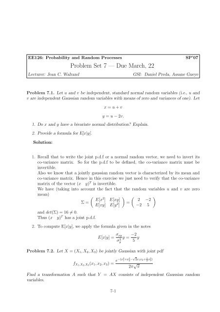
EE126: Probability and Random Processes<br />
SP’07<br />
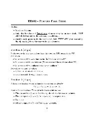
<strong>Problem</strong> <strong>Set</strong> 7 — <strong>Due</strong> <strong>March</strong>, <strong>22</strong><br />
Lecturer: Jean C. Walrand<br />
GSI: Daniel Preda, Assane Gueye<br />
<strong>Problem</strong> 7.1. Let u and v be independent, standard normal random variables (i.e., u and<br />
v are independent Gaussian random variables with means of zero and variances of one). Let<br />
x = u + v<br />
y = u − 2v.<br />
1. Do x and y have a bivariate normal distribution? Explain.<br />
2. Provide a formula for E[x|y].<br />
Solution:<br />
1. Recall that to write the joint p.d.f or a normal random vector, we need to invert its<br />
co-variance matrix. So for the p.d.f to be defined, the co-variance matrix must be<br />
invertible.<br />
Also we know that a jointly gaussian random vector is characterized by its mean and<br />
co-variance matrix. Hence in this exercise we just need to verify that the co-variance<br />
matrix of the vector (x y) T is invertible.<br />
We have (taking into account the fact that the random variables u and v are zero<br />
mean)<br />
( ) ( )<br />
E[x<br />
Σ =<br />
2 ] E[xy] 2 −2<br />
E[xy] E[y 2 =<br />
] −2 5<br />
and det(Σ) = 16 ≠ 0.<br />
Thus (x y) T has a joint p.d.f.<br />
2. To compute E[x|y], we apply the formula given in the notes<br />
E[x|y] = σ xy<br />
y = −2<br />
σy<br />
2 5 y<br />
<strong>Problem</strong> 7.2. Let X = (X 1 , X 2 , X 3 ) be jointly Gaussian with joint pdf<br />
f X1 ,X 2 ,X 3<br />
(x 1 , x 2 , x 3 ) = e−(x2 1 +x2 2 −√ 2x 1 x 2 + 1 2 x2 3 )<br />
2π √ π<br />
Find a transformation A such that Y = AX consists of independent Gaussian random<br />
variables.<br />
7-1
EE126 <strong>Problem</strong> <strong>Set</strong> 7 — <strong>Due</strong> <strong>March</strong>, <strong>22</strong> SP’07<br />
Solution:<br />
In class we have seen that any jointly gaussian random vector X can be written as X = BY<br />
where Y has i.i.d standard normal components, and BB T = Σ X . A formal way to compute B<br />
is to use the eigenvalue decomposition of the matrix Σ X = UDU T where U is an orthogonal<br />
matrix and D is a diagonal matrix with non-negative entries in the diagonal. From this, B<br />
can be written B = D 1 2 U. And, if Σ X is invertible, A can be chosen as A = B −1 = UD − 1 2 .<br />
If you are not familiar with eigenvalue decomposition, you can still compute B by solving<br />
the matrix equation BB T = Σ X .<br />
First let’s figure out what Σ X is. For that, notice that<br />
f X1 ,X 2 ,X 3<br />
(x 1 , x 2 , x 3 ) =<br />
1<br />
√<br />
(2π)2 |Σ X | e− 1 2 (x 1,x 2 ,x 3 )Σ −1<br />
X (x 1,x 2 ,x 3 ) T<br />
Developing the term in the exponent and identifying with the p.d.f given in the exercise,<br />
yield to<br />
⎛<br />
Σ X = BB T = ⎝<br />
which gives<br />
2 − √ 2 0<br />
− √ 2 2 0<br />
0 0 1<br />
⎞<br />
⎛<br />
⎠ = ⎝<br />
⎛<br />
A = B −1 = ⎝<br />
−1.3066 0.5412 0<br />
1.3066 0.5412 0<br />
0 0 1<br />
−0.3827 0.3827 0<br />
0.9239 0.9239 0<br />
0 0 1<br />
⎞ ⎛<br />
⎠ ⎝<br />
−1.3066 0.5412 0<br />
1.3066 0.5412 0<br />
0 0 1<br />
Note:<br />
Here, we have solved the exercise for Y having i.i.d standard normal components. . . but<br />
independent is enough and probably easier!<br />
<strong>Problem</strong> 7.3. A signal of amplitude s = 2 is transmitted from a satellite but is corrupted<br />
by noise, and the received signal is Z = s + W , where W is noise. When the weather is<br />
good, W is normal with zero mean and variance 1. When the weather is bad, W is normal<br />
with zero mean and variance 4. Good and bad weather are equally likely. In the absence of<br />
any weather information:<br />
1. Calculate the PDF of Z.<br />
2. Calculate the probability that Z is between 1 and 3.<br />
Solution:<br />
⎞<br />
⎠<br />
⎞<br />
⎠<br />
T<br />
1. Let G represent the event that the weather is good. We are given P (G) = 1 2 .<br />
To find the PDF of X, we first find the PDF of W , since X = s + W = 2 + W . We<br />
know that given good weather, W ∼ N(0, 1). We also know that given bad weather,<br />
7-2
EE126 <strong>Problem</strong> <strong>Set</strong> 7 — <strong>Due</strong> <strong>March</strong>, <strong>22</strong> SP’07<br />
W ∼ N(0, 4). To find the unconditional PDF of W , we use the density version of the<br />
total probability theorem.<br />
f W (w) = P (G) · f W |G (w) + P (G c ) · f W |G c(w)<br />
= 1 2 · 1<br />
√ e − w2<br />
2 + 1 2π 2 · 1<br />
2 √ w2<br />
e− 2(4)<br />
2π<br />
We now perform a change of variables using X = 2 + W to find the PDF of X:<br />
f X (x) = f W (x − 2) = 1 2 ·<br />
1<br />
√<br />
2π<br />
e − (x−2)2<br />
2 + 1 2 ·<br />
1<br />
2 √ 2π<br />
e−<br />
(x−2)2<br />
8 .<br />
2. In principle, one can use the PDF determined in part (a) to compute the desired<br />
probability as<br />
∫ 3<br />
1<br />
f X (x) dx.<br />
It is much easier, however, to translate the event {1 ≤ X ≤ 3} to a statement about<br />
W and then to apply the total probability theorem.<br />
P (1 ≤ X ≤ 3) = P (1 ≤ 2 + W ≤ 3) = P (−1 ≤ W ≤ 1)<br />
We now use the total probability theorem.<br />
P (−1 ≤ W ≤ 1) = P (G) P (−1 ≤ W ≤ 1 | G) +P (G c ) P (−1 ≤ W ≤ 1 | G c )<br />
} {{ } } {{ }<br />
a<br />
b<br />
Since conditional on either G or G c the random variable W is Gaussian, the conditional<br />
∫<br />
probabilities a and b can be expressed using Φ (Φ(x) = √ 1 ∞<br />
2π x<br />
on G, we have W ∼ N(0, 1) so<br />
a = Φ(1) − Φ(−1) = 2Φ(1) − 1.<br />
Try to show that Φ(−x) = 1 − Φ(x)!<br />
Conditional on G c , we have W ∼ N(0, 4) so<br />
( ( 1<br />
b = Φ − Φ −<br />
2)<br />
1 )<br />
2<br />
The final answer is thus<br />
P (1 ≤ X ≤ 3) = 1 2 (2Φ (1) − 1) + 1 2<br />
( 1<br />
= 2Φ − 1.<br />
2)<br />
x2<br />
e−<br />
( ( ) 1<br />
2Φ − 1 .<br />
2)<br />
2 dx). Conditional<br />
<strong>Problem</strong> 7.4. Suppose X, Y are independent gaussian random variables with the same<br />
variance. Show that X − Y and X + Y are independent.<br />
7-3
EE126 <strong>Problem</strong> <strong>Set</strong> 7 — <strong>Due</strong> <strong>March</strong>, <strong>22</strong> SP’07<br />
Solution:<br />
First note that, in general, to show that two random variables U and V are independent,<br />
we need to show that<br />
P (U ∈ (u 1 , u 2 ), V ∈ (v 1 , v 2 )) = P (U ∈ (u 1 , u 2 ))P (V ∈ (v 1 , v 2 )), ∀u 1 , u 2 , v 1 , v 2<br />
which can be very hard sometimes.<br />
And also in general un-correlation is weaker than independence.<br />
However for Gaussian random variables, we know that independence is equivalent to uncorrelation.<br />
So, to show that U and V are independent, it suffices to show that they are<br />
un-correlated:<br />
E[(U − E(U))(V − E[V ])] = 0<br />
We will apply this to U = X + Y and V = X − Y . First notice that E[U] = E[X] + E[Y ]<br />
and E[V ] = E[X] − E[Y ]. Thus<br />
E[X + Y − (E[X] + E[Y ])(X − Y − (E[X] − E[Y ])] = E[(X − E[X]) 2 ] − E[(Y − E[Y ]) 2 ]<br />
+E[(X − E[X])(Y − E[Y ])]<br />
−E[(X − E[X])(Y − E[Y ])]<br />
= E[(X − E[X]) 2 ] − E[(Y − E[Y ]) 2 ]<br />
= 0<br />
because X and Y have equal variance.<br />
So X −Y and X +Y are uncorrelated; since they are jointly gaussian (because they are linear<br />
combinations of the same independent random variables X and Y ), they are independent.<br />
<strong>Problem</strong> 7.5. Steve is trying to decide how to invest his wealth in the stock market. He<br />
decides to use a probabilistic model for the shares price changes. He believes that, at the<br />
end of the day, the change of price Z i of a share of a particular company i is the sum of<br />
two components: X i , due solely to the performance of the company, and the other Y due to<br />
investors’ jitter.<br />
Assuming that Y is a normal random variable, zero-mean and with variance equal to 1,<br />
and independent of X i . Find the PDF of Z i under the following circumstances in part a) to<br />
c),<br />
1. X 1 is Gaussian with a mean of 1 dollar and variance equal to 4.<br />
2. X 2 is equal to -1 dollars with probability 0.5, and 3 dollars with probability 0.5.<br />
3. X 3 is uniformly distributed between -2.5 dollars and 4.5 dollars (No closed form expression<br />
is necessary.)<br />
7-4
EE126 <strong>Problem</strong> <strong>Set</strong> 7 — <strong>Due</strong> <strong>March</strong>, <strong>22</strong> SP’07<br />
4. Being risk averse, Steve now decides to invest only in the first two companies. He<br />
uniformly chooses a portion V of his wealth to invest in company 1 (V is uniform<br />
between 0 and 1.) Assuming that a share of company 1 or 2 costs 100 dollars, what is<br />
the expected value of the relative increase/decrease of his wealth?<br />
Solution:<br />
1. Because Z 1 is the sum of two independent Gaussian random variables, X 1 and Y , the<br />
PDF of Z 1 is also Gaussian. The mean and variance of Z 1 are equal to the sums of the<br />
expected values of X 1 and Y and the sums of the variances of X 1 and Y , respectively.<br />
f Z1 (z 1 ) = N(1, 5)<br />
2. X 2 is a two-valued discrete random variable, so it is convenient to use the total probability<br />
theorem and condition the PDF of Z 2 on the outcome of X 2 . Because linear<br />
transformations of Gaussian random variables are also Gaussian, we obtain:<br />
f Z2 (z 2 ) = 1 2 N(−1, 1) + 1 N(3, 1)<br />
2<br />
3. We can use convolution here to get the PDF of Z 3 .<br />
f Z3 (z 3 ) =<br />
∫ ∞<br />
−∞<br />
N(0, 1)f X3 (z 3 − y)dy<br />
Using the fact that X 3 is uniform from -2.5 to 4.5, we can reduce this convolution to:<br />
f Z3 (z 3 ) =<br />
∫ z3 +2.5<br />
z 3 −4.5<br />
N(0, 1) 1 7 dy<br />
A normal table is necessary to compute this integral for all values of z 3 .<br />
4. Given an experimental value V = v, we can draw the following tree:<br />
E[Z] = E[E[Z | V ]] =<br />
7-5<br />
∫ 1<br />
0<br />
E[Z | V = v]f V (v)dv
EE126 <strong>Problem</strong> <strong>Set</strong> 7 — <strong>Due</strong> <strong>March</strong>, <strong>22</strong> SP’07<br />
E[Z | V = v] = v · 1 + (1 − v)[−1 · 1<br />
2 + 3 · 1 ] = v + (1 − v) = 1<br />
2<br />
Plugging E[Z | V = v] and f V (v) = 1 into our first equation, we get<br />
E[Z] =<br />
∫ 1<br />
0<br />
1 · 1dv = 1.<br />
Since the problem asks for the relative change in wealth, we need to divide E[Z] by<br />
100. Thus the expected relative change in wealth is 1 percent.<br />
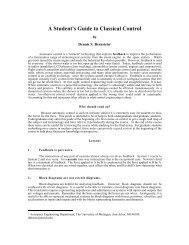
<strong>Problem</strong> 7.6. The Binary Phase-shift Keying (BPSK) and Quadrature Phase-shift Keying<br />
(QPSK) modulation schemes are shown in figure 7.1. We consider that in both cases, the<br />
symbols (S) are sent over an additive gaussian channel with zero mean and variance σ 2 .<br />
Assuming that the symbols are equally likely, compute the average error probability for each<br />
scheme. Which one is better?<br />
QPSK<br />
BPSK<br />
S0<br />
s1<br />
-a<br />
a<br />
S1<br />
S2<br />
-a<br />
a<br />
S2<br />
S3<br />
Figure 7.1. QPSK and BPSK modulations<br />
Solution:(Hint)<br />
Note that the comparison is not fair because the two schemes do not have the same rate<br />
(eggs and apples!). But let us compute the error probabilities and compare them.<br />
In both cases, an error occurs when one symbol is sent and the receiver decides for a different<br />
one. Since the symbols are equally likely, the decoding (or decision) rule will be to decide in<br />
favor of the symbol S i that maximizes the likelihood (assuming that Y is the received signal)<br />
f Y (y|S i ) =<br />
1<br />
√ e − (y−S i )T ·(y−S i )<br />
2·2<br />
2π · 2<br />
where S i ∈ {−a, a} for BPSK and S i ∈ {(−a, −a), (−a, a), (a, −a), (a, a)}.<br />
It is not hard to see that maximizing the likelihood is the same as minimizing |y − S i )| 2<br />
which turns out to be the Euclidean distance between the received point and the symbol S i .<br />
Thus the decision rule is as follows (assuming that Z ∼ N(0, 2) is the channel noise):<br />
7-6
EE126 <strong>Problem</strong> <strong>Set</strong> 7 — <strong>Due</strong> <strong>March</strong>, <strong>22</strong> SP’07<br />
• BPSK: decide for a if X = S + Z ≥ 0 and decide for −a otherwise. Error occurs if<br />
S = a (S = −a) and X = a + Z < 0 ⇔ Z < −a (X = −a + Z ≥ 0 ⇔ Z ≥ a).<br />
The corresponding conditional probabilities are P (Z < −a) = Φ( √ 2a) (P (Z ≥ a) =<br />
Φ( √ 2a)), thus the average error probability is Φ( √ 2a) for BPSK.<br />
• QPSK: decide for (a, a) if X is in the first quartan, (−a, a) if X is in the second quartan,<br />
etc...<br />
For QPSK (which can be modeled as 2 independent BPSK), let’s assume that signal<br />
S 1 = (a, a) was sent. Observe that error occurs if the received signal does not fall in<br />
the first quartan. By considering the probability of detecting any other signal, we can<br />
see that given S 1 was sent the error probability is equal to<br />
P qpsk<br />
e = Φ(2a) + 2Φ( √ 2a)<br />
which is the average error probability given the symmetry of the problem.<br />
For a large enough we have Pe<br />
qpsk ≈ 2Pe<br />
bpsk<br />
<strong>Problem</strong> 7.7. When using a multiple access communication channel, a certain number of<br />
users N try to transmit information to a single receiver. If the real-valued random variable<br />
X i represents the signal transmitted by user i, the received signal Y is<br />
Y = X 1 + X 2 + · · · + X N + Z,<br />
where Z is an additive noise term that is independent of the transmitted signals and is<br />
assumed to be a zero-mean Gaussian random variable with variance σZ 2 . We assume that<br />
the signals transmitted by different users are mutually independent and, furthermore, we<br />
assume that they are identically distributed, each Gaussian with mean µ and variance σX 2 .<br />
1. If N is deterministically equal to 2, find the transform or the PDF of Y .<br />
2. In most practical schemes, the number of users N is a random variable. Assume now<br />
that N is equally likely to be equal to 0, 1, . . . , 10.<br />
(a) Find the transform or the PDF of Y .<br />
(b) Find the mean and variance of Y .<br />
(c) Given that N ≥ 2, find the transform or PDF of Y .<br />
Solution:<br />
1. Here it is easier to find the PDF of Y . Since Y is the sum of independent Gaussian<br />
random variables, Y is Gaussian with mean 2µ and variance 2σ 2 X + σ2 Z .<br />
7-7
EE126 <strong>Problem</strong> <strong>Set</strong> 7 — <strong>Due</strong> <strong>March</strong>, <strong>22</strong> SP’07<br />
2. (a) The transform of N is<br />
Since Y is the sum of<br />
M N (s) = 1 11 (1 + es + e 2s + · · · + e 10s ) = 1<br />
11<br />
• a random sum of Gaussian random variables<br />
• an independent Gaussian random variable,<br />
∑10<br />
e ks<br />
k=0<br />
M Y (s) =<br />
=<br />
(<br />
) ( 1<br />
M N (s)| e s =M X (s) M Z (s) =<br />
11<br />
( 1<br />
11<br />
= 1<br />
11<br />
∑10<br />
k=0<br />
10<br />
∑<br />
k=0<br />
e skµ+ s2 kσ<br />
X<br />
2<br />
2<br />
e skµ+ s2 (kσ<br />
X 2 +σ2 Z )<br />
2<br />
)<br />
e s2 σ<br />
Z<br />
2<br />
2<br />
∑10<br />
(e sµ+ s2 σ<br />
X<br />
2<br />
k=0<br />
2 ) k )<br />
In general, this is not the transform of a Gaussian random variable.<br />
e s2 σ<br />
Z<br />
2<br />
2<br />
(b) One can differentiate the transform to get the moments, but it is easier to use the<br />
laws of iterated expectation and conditional variance:<br />
EY = EXEN + EZ = 5µ<br />
var(Y ) = ENvar(X) + (EX 2 )var(N) + var(Z) = 5σ 2 X + 10µ 2 + σ 2 Z<br />
(c) Now, the new transform for N is<br />
Therefore,<br />
M Y (s) =<br />
=<br />
= 1 9<br />
M N (s) = 1 9 (e2s + · · · + e 10s ) = 1 9<br />
(<br />
) ( 1<br />
M N (s)| e s =M X (s) M Z (s) =<br />
9<br />
( 1<br />
9<br />
∑10<br />
k=2<br />
10<br />
e skµ+ s2 (kσ<br />
X 2 +σ2 Z )<br />
2<br />
∑<br />
k=2<br />
e skµ+ s2 kσ<br />
X<br />
2<br />
2<br />
)<br />
e s2 σ<br />
Z<br />
2<br />
2<br />
∑10<br />
e ks<br />
k=2<br />
∑10<br />
(e sµ+ s2 σ<br />
X<br />
2<br />
k=2<br />
2 ) k )<br />
e s2 σ<br />
Z<br />
2<br />
2<br />
7-8