Apr. 20: Hartree-Fock-Bogoliubov, BCS
Apr. 20: Hartree-Fock-Bogoliubov, BCS
Apr. 20: Hartree-Fock-Bogoliubov, BCS

Create successful ePaper yourself
Turn your PDF publications into a flip-book with our unique Google optimized e-Paper software.
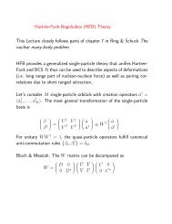
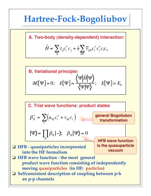
<strong>Hartree</strong>-<strong>Fock</strong>-<strong>Bogoliubov</strong><br />
A. Two-body (density-dependent) interaction:<br />
H ˆ = ! t ij<br />
c + i<br />
c j<br />
+ 1 4! v ijkl<br />
c + i<br />
c + j<br />
c l<br />
c k<br />
ij<br />
ijkl<br />
B. Variational principle:<br />
!E["] = 0; E ["] = " ˆ<br />
H "<br />
" " ; E "<br />
[ ] > E 0<br />
C. Trial wave functions: product states<br />
"( )<br />
! K + = u iK<br />
c i + + v iK<br />
c i<br />
i<br />
# = $ ! K<br />
% ; ! K<br />
# = 0<br />
K<br />
❏ HFB - quasiparticles incorporated<br />
into the HF formalism<br />
❏ HFB wave function - the most general<br />
general <strong>Bogoliubov</strong><br />
transformation<br />
HFB wave function<br />
is the quasuparticle<br />
vacuum<br />
product wave function consisting of independently<br />
moving quasiparticles (in HF: particles)<br />
❏ Selfconsistent description of coupling between p-h<br />
an p-p channels
HFB - density matrix and pairing tensor<br />
HFB density matrix<br />
HFB pairing tensor<br />
! ij<br />
" # c j + c i<br />
# , $ ij<br />
" # c j<br />
c i<br />
#<br />
ˆ ! = v * v T , $ ˆ = v * u T<br />
ˆ ! 2 % ˆ ! = % $ ˆ $ ˆ<br />
+ , ˆ ! $ ˆ = $ ˆ ˆ !<br />
ˆ ! =<br />
%<br />
'<br />
&<br />
ˆ " # ˆ<br />
$ # ˆ<br />
1 $ ˆ<br />
" *<br />
(<br />
*, ! ˆ 2 = ! ˆ<br />
)<br />
! ˆ % u K(<br />
' * = 0, ! ˆ v *<br />
% (<br />
K<br />
' *<br />
& v K ) & u K )<br />
* = v *<br />
% (<br />
'<br />
K<br />
* *<br />
& u K )<br />
Generalized<br />
density matrix<br />
Eigenvalues are 0 or 1 (thus<br />
defining occupations of<br />
quasiparticle states)<br />
ˆ H (c + ,c) ! ˆ H (" + ,") = E 0<br />
+ ˆ H <strong>20</strong><br />
+ ˆ H 11<br />
+ ˆ H int<br />
Independent quasiparticle<br />
Hamiltonian (H HFB )<br />
[ H ˆ , N ˆ ] = 0, but H ˆ<br />
HFB<br />
, N ˆ<br />
[ ] ! 0<br />
Quasiparticle<br />
interaction<br />
However, we require that ˆ N = N " ˆ H ' = ˆ H # $ ˆ N
HFB equations<br />
ˆ K =<br />
$ h ˆ ! "<br />
&<br />
%<br />
! ˆ # * ! ˆ<br />
h ij<br />
= t ij<br />
+ * ij<br />
# ˆ '<br />
)<br />
h * + "(<br />
* ij<br />
= + v iljk<br />
, kl<br />
kl<br />
# ij<br />
= 1 2 + v ijkl<br />
- kl<br />
kl<br />
HFB Hamiltonian<br />
HF Hamiltonian<br />
Selfconsistent HF field<br />
Selfconsistent pair field<br />
HFB equations<br />
$ h ˆ ! "<br />
&<br />
%<br />
! ˆ # * ! ˆ<br />
# ˆ ' $<br />
) u K'<br />
$ u<br />
& ) = E<br />
K '<br />
h * K & )<br />
+ "(%<br />
v K ( % v K (<br />
[ K ˆ , . ˆ ] = 0<br />
Complicated<br />
eigenvalue problem<br />
❏ HFB equations treat p-h and p-p on the same footing<br />
❏ Δ is a state-dependent field. In general, it depends on<br />
density and has a kinetic term<br />
❏ The generalized density matrix and the HFB Hamiltonian<br />
can be diagonalized simultaneously<br />
❏ Fermi level determined from the particle number<br />
equation<br />
❏ Often it is convenien to express the HFB equations<br />
in the canonical basis
Independent quasiparticle approach<br />
! k + = u k<br />
c k + " v k<br />
c k<br />
! + k<br />
= u k<br />
c + k<br />
+ v k<br />
c k<br />
<strong>Bogoliubov</strong>-<br />
Valatin<br />
Transformation<br />
phase convention: u k<br />
= u k<br />
> 0,<br />
ε<br />
v k<br />
= "v k<br />
> 0<br />
F<br />
+<br />
{! k<br />
,! j } = 0, ! k+<br />
,! j<br />
+<br />
{! k<br />
,! j } = # ij<br />
$ u 2 k<br />
+ v 2 k<br />
=1<br />
{ } = 0,<br />
( )<br />
0 = <strong>BCS</strong> = u k<br />
+ v k<br />
c + +<br />
! k<br />
c k<br />
"<br />
# k<br />
0 = 0<br />
0 ! exp A +<br />
A + =<br />
u k<br />
k > 0<br />
v k<br />
k >0<br />
( ) " =<br />
$ c k<br />
+ +<br />
c k<br />
#<br />
1<br />
n!<br />
n= 0<br />
$ A +<br />
( ) n "<br />
<strong>BCS</strong> wave function is<br />
the quasiparticle<br />
vacuum!<br />
<strong>BCS</strong> function is a<br />
superposition of<br />
different number of pairs<br />
❏ Important ground-state correlations are included<br />
❏ <strong>BCS</strong> wave function does not have a sharp particle<br />
number (an intrinsic wave function!)
<strong>BCS</strong> equations<br />
ˆ H (c + ,c) ! ˆ H (" + ,") = E 0<br />
+ ˆ H <strong>20</strong><br />
+ ˆ H 11<br />
+ ˆ H int<br />
Independent quasiparticle<br />
Hamiltonian (H <strong>BCS</strong> )<br />
Quasiparticle<br />
interaction<br />
[ H ˆ , N ˆ ] = 0, but H ˆ<br />
<strong>BCS</strong><br />
, N ˆ<br />
[ ] ! 0<br />
However, we require that ˆ N = N " ˆ H ' = ˆ H # $ ˆ N<br />
Particle number<br />
equation<br />
Variational method<br />
! 0 ˆ H ' 0 = 0<br />
˜ " k<br />
= " k<br />
+ # v k ki i<br />
v 2 i<br />
$ %<br />
i > 0<br />
!<br />
N = 2v i<br />
2<br />
i > 0<br />
" k<br />
= #! v kk ii<br />
u i<br />
v i<br />
i >0<br />
v 2 k<br />
= 1 $<br />
2<br />
&<br />
%<br />
1 !<br />
˜ " k<br />
˜ " 2 2<br />
k<br />
+ # k<br />
'<br />
)<br />
(<br />
Pairing gap<br />
equation
<strong>BCS</strong> model<br />
H ˆ<br />
<strong>BCS</strong><br />
! + k1<br />
! + k 2<br />
L! + k n<br />
0 = (E 0<br />
+ E k1<br />
+ E k2<br />
+L+ E k n<br />
)! + k 1<br />
! + k 2<br />
L! + kn<br />
0<br />
E k<br />
=<br />
˜ ! 2 2<br />
k<br />
+ " k<br />
Quasiparticle energy<br />
State-independent monopole pairing force:<br />
V ˆ<br />
pair<br />
= !GP ˆ + P ˆ = !G " c + i<br />
c + i<br />
c j<br />
c j<br />
i, j > 0<br />
P ˆ # c + +<br />
" i<br />
c i<br />
v ijkl<br />
= !G$ ji<br />
$ lk<br />
sgn( j)sgn(k)<br />
i> 0<br />
( )<br />
'<br />
% = G" u i<br />
v i<br />
& %)<br />
G<br />
i> 0 ( 2<br />
"<br />
i > 0<br />
1 *<br />
!1, = 0<br />
E i +<br />
❏ Fermi level can be extracted from<br />
experimental binding energies:<br />
❏ Energy gap in even-even nuclei:<br />
❏ High level density in odd systems:<br />
! = dE<br />
dN<br />
E k1<br />
+ E k2<br />
! 2"<br />
E k<br />
! E k0<br />
" ˜ # k 2 + $ 2 ! $<br />
❏ Pairing gap can be extraxted from experimental<br />
odd-even mass differences:<br />
[ ]<br />
! " # 1 (N +<br />
2 E 2) (<br />
g.s .<br />
+ E N) (N +1)<br />
g.s.<br />
# 2E g.s.
The gap equation<br />
❏ Schematic solution for the case of uniform<br />
density of single-particle states<br />
2<br />
G = ! 1<br />
"1 = G 2<br />
k > 0<br />
E k<br />
b<br />
1<br />
% g (#<br />
)d#<br />
# 2 + $ 2<br />
a<br />
((1/ g G)<br />
If g (#<br />
) & g and Gg
Simple pairing model<br />
+ε<br />
-ε<br />
+ε<br />
+<br />
-ε<br />
Ω times<br />
+ ...<br />
N = 2! particles " # = 0 (assuming Gv 2 < $)<br />
1<br />
G = ! E " % = $<br />
&<br />
(<br />
'<br />
G<br />
G crit<br />
2<br />
)<br />
+<br />
*<br />
,1, G crit<br />
= $ !<br />
Δ<br />
Normal phase<br />
Correlations<br />
beyond <strong>BCS</strong><br />
Superconductor<br />
Phase transition<br />
G crit<br />
G<br />
❏ Correlations are important, especially<br />
for small values of G<br />
❏ Static description breaks down when the<br />
single-particle level density is small
Recall that v 2 k is the occupation probability for state k. Thus, the<br />
pairing interaction destabilizes the Fermi surface!<br />
Inserting these results into Eq. (1) yields the Gap Equation<br />
∆ k = − 1 2<br />
∑<br />
v kkll<br />
l>0<br />
∆ k<br />
√˜ε<br />
2<br />
k + ∆ 2 k<br />
This equation, together with the Equation for the energies ˜ε k has to<br />
be solved iteratively.<br />
Simple examples and illustration:<br />
(1) Pure pairing force: v ijkl = −G, t k,l = δ kl ε l<br />
Gap equation<br />
∆ = G 2<br />
∑<br />
l>0<br />
∆<br />
√<br />
(εk − µ) 2 + ∆ 2 k<br />
For vanishing single-particle energies ε k = 0 and a single-j shell one<br />
recovers the results of the seniority model. The gap becomes<br />
√<br />
∆ = G<br />
n √<br />
2<br />
⎛<br />
⎝Ω − N 2<br />
⎞<br />
⎠ = GΩ<br />
2<br />
at half filling. Comparison with the seniority model shows that 2∆ is<br />
the energy to break a pair and equals the excitation energy!
(2) Analytical solution for simple model.<br />
Assume constant interaction G, constant gap ∆, and constant density<br />
of states ρ, and restrict summation to the vicinity δ of the Fermi<br />
surface. Gap equation:<br />
1 = G 2<br />
µ+δ ∫<br />
µ−δ<br />
For weak pairing Gρ ≪ 1 one finds<br />
ρ(ε)<br />
dε√ (ε − µ)2 + ∆ = Gρ arsinh δ 2 ∆<br />
⎛<br />
∆<br />
δ ∝ exp ⎜<br />
−1<br />
⎝<br />
|G|ρ<br />
Gap is nonperturbative in interaction G!<br />
The particle number variance is<br />
(∆N) 2 ≈ 2ρ∆ atan δ ⎧<br />
⎪⎨<br />
∆ = πρ∆ for weak pairing ∆ ≪ δ,<br />
⎪ ⎩ 2ρδ for strong pairing.<br />
⎞<br />
⎟<br />
⎠
<strong>BCS</strong> essentials<br />
1. The Fermi surface of a Fermi gas is unstable with respect to attractive<br />
interactions. The gap equation has a nontrivial solution<br />
∆ ≠ 0 whenever the interaction or the density of states is sufficiently<br />
large.<br />
2. The finite excitation gap causes superfluidity: The system cannot<br />
absorb arbitrarily small perturbations and therefore remains inert<br />
(See, e.g., Landau & Lifshitz, Statistical Mechanics II).