Psychology 2020 Introduction to Psychological Methods
Psychology 2020 Introduction to Psychological Methods
Psychology 2020 Introduction to Psychological Methods

Create successful ePaper yourself
Turn your PDF publications into a flip-book with our unique Google optimized e-Paper software.
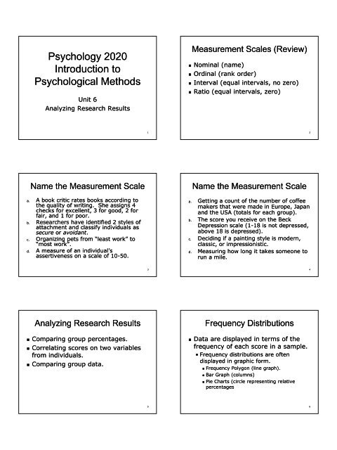
<strong>Psychology</strong> <strong>2020</strong><br />
<strong>Introduction</strong> <strong>to</strong><br />
<strong>Psychological</strong> <strong>Methods</strong><br />
Unit 6<br />
Analyzing Research Results<br />
Measurement Scales (Review)<br />
• Nominal (name)<br />
• Ordinal (rank order)<br />
• Interval (equal intervals, no zero)<br />
• Ratio (equal intervals, zero)<br />
1<br />
2<br />
Name the Measurement Scale<br />
a. A book critic rates books according <strong>to</strong><br />
the quality of writing. She assigns 4<br />
checks for excellent, 3 for good, 2 for<br />
fair, and 1 for poor.<br />
b. Researchers have identified 2 styles of<br />
attachment and classify individuals as<br />
secure or avoidant.<br />
c. Organizing pets from “least work” <strong>to</strong><br />
“most work”.<br />
d. A measure of an individual’s<br />
assertiveness on a scale of 10-50.<br />
Name the Measurement Scale<br />
a. Getting a count of the number of coffee<br />
makers that were made in Europe, Japan<br />
and the USA (<strong>to</strong>tals for each group).<br />
b. The score you receive on the Beck<br />
Depression scale (1-1818 is not depressed,<br />
above 18 is depressed).<br />
c. Deciding if a painting style is modern,<br />
classic, or impressionistic.<br />
d. Measuring how long it takes someone <strong>to</strong><br />
run a mile.<br />
3<br />
4<br />
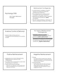
Analyzing Research Results<br />
• Comparing group percentages.<br />
• Correlating scores on two variables<br />
from individuals.<br />
• Comparing group data.<br />
Frequency Distributions<br />
• Data are displayed in terms of the<br />
frequency of each score in a sample.<br />
• Frequency distributions are often<br />
displayed in graphic form.<br />
• Frequency Polygon (line graph).<br />
• Bar Graph (columns)<br />
• Pie Charts (circle representing relative<br />
percentages<br />
5<br />
6
Frequency Polygon<br />
Bar Graph<br />
<strong>Psychology</strong> Grades<br />
<strong>Psychology</strong> Grades<br />
Frequency<br />
y12<br />
8<br />
4<br />
0<br />
A B C D F<br />
Course Grades<br />
Frequency<br />
12<br />
8<br />
4<br />
0<br />
A B C D F<br />
Course Grades<br />
7<br />
8<br />
Pie Chart<br />
Descriptive Statistics<br />
<strong>Psychology</strong> Grades<br />
F<br />
8%<br />
D<br />
0%<br />
A<br />
C<br />
36%<br />
24%<br />
B<br />
32%<br />
Course Grades<br />
• Descriptive statistics quantitatively<br />
summarize a data set.<br />
• Two numbers are usually reported<br />
• A measure of central tendency<br />
• A measure variability<br />
9<br />
10<br />
Measures of Central Tendency<br />
Practice Calculations<br />
• Mean<br />
• Total divided by the number of scores<br />
• Median<br />
• Middle score after scores have been<br />
arranged in numerical order from<br />
highest <strong>to</strong> lowest<br />
• Mode<br />
• Most frequently occurring score<br />
11<br />
• Data set values: 10, 13, 6, 23, 18, 25,<br />
54, 54<br />
• Mean =<br />
• 10+13+6+23+18+25+54+54=203<br />
•203/8= 203/8=25.3825.38<br />
• Median =<br />
• 6,10,13,18,23,25,54,54<br />
,25,54,54<br />
(18+23)/2=20.520.5<br />
• Mode =<br />
•54<br />
12
Measures of Variability<br />
• Variance or s 2<br />
• The average squared deviation of scores from<br />
the mean<br />
• Standard Deviation or s<br />
• The square root of the variance which gives<br />
you the average deviation of scores from the<br />
mean<br />
• Range<br />
• The difference between the highest and lowest<br />
scores in a group.<br />
Practice Calculations<br />
• Data set values: 10, 13, 6, 23, 18, 25,<br />
54, 54<br />
• Range =<br />
• 54-6=<br />
6=48<br />
13<br />
14<br />
Correlation Coefficients<br />
• Statistics that describe the strength of the<br />
relation between two or more variables.<br />
• Pearson Product-Moment Correlation<br />
Coefficient (r)<br />
• Linear relationships between interval or ratio data.<br />
• Higher the number the stronger the correlation<br />
• + or – before the number indicates a positive or<br />
negative correlation.<br />
• Squaring the r value yields the percentage of shared<br />
variance accounted for by the measured variables<br />
• See the correlation<br />
Effect Size<br />
• Measures the strength of an<br />
independent variable manipulation.<br />
• Effect size correlations<br />
•.10 <strong>to</strong> .20 small effect<br />
• .30 medium effects<br />
• .40 and above are considered strong<br />
effects<br />
15<br />
16<br />
Statistical Significance<br />
• If the difference between group scores is largely<br />
due <strong>to</strong> the IV manipulation and not chance we<br />
say they are “significant”.<br />
• Statistics allow us <strong>to</strong> determine how significant<br />
they are compared <strong>to</strong> what we would expect by<br />
chance alone.<br />
• Statically significant means that we have<br />
analyzed our data with an inferential statistic and<br />
found differences that would be expected by<br />
chance less than 5% of the time if the<br />
experiment were repeated several times.<br />
Regression Equations<br />
• These are used <strong>to</strong> predict a person’s score on one<br />
variable when we know their score on another<br />
variable.<br />
• Predic<strong>to</strong>r variable is the known score<br />
• Criterion variable is the score <strong>to</strong> be predicted<br />
• Multiple Correlations make predictions of the<br />
value of the criterion variable using more than<br />
one predic<strong>to</strong>r variable.<br />
17<br />
18
Partial Correlations<br />
• The correlation of two variables with the<br />
effects of a third variable statistically<br />
removed.<br />
• This method helps the researcher<br />
understand more clearly how the<br />
relationship between two variables is<br />
influenced by other variables.<br />
Structural Models<br />
• These methods give more<br />
information than simple correlation<br />
or partial correlation methods.<br />
• They indicate “paths of effect” of<br />
proposed causal sequences and the<br />
effect strength of each variable in<br />
the sequence.<br />
19<br />
20<br />
Practice Activity<br />
• Arrange these correlation coefficients<br />
from weakest correlation <strong>to</strong><br />
strongest correlation:<br />
.45, .21, -.56, .02, -.98, .76, -.87, .13<br />
Two Hypotheses<br />
• Null Hypothesis<br />
• The observed difference is due <strong>to</strong><br />
random error.<br />
• Research Hypothesis<br />
• The observed difference is due <strong>to</strong> the<br />
manipulation of the independent<br />
variable.<br />
21<br />
22<br />
The Logic of the Null Hypothesis<br />
• The goal of an experiment is <strong>to</strong> show the<br />
null hypothesis is false.<br />
• The research hypothesis is never “proven”<br />
but only supported.<br />
• Results are always discussed in terms of<br />
the probability that the observed<br />
differences could have been produced by<br />
random error.<br />
Interpreting Research Results<br />
• What is the probability that the difference<br />
in group means is due <strong>to</strong> chance<br />
variability?<br />
• Inferential statistics help us calculate<br />
and compare variability caused by the<br />
IV manipulation with chance variability.<br />
• This allows us <strong>to</strong> generalize our results<br />
from our sample <strong>to</strong> our populations.<br />
• Examples of inferential statistics are t-<br />
tests and analyses of variance (F-tests)<br />
23<br />
24
T-TestsTests<br />
• T-tests compare the difference<br />
between the two group means <strong>to</strong> the<br />
variability found in each group<br />
(within-group variability).<br />
t =<br />
X − X<br />
2<br />
2<br />
s s2<br />
+<br />
N N<br />
1<br />
2<br />
1<br />
1<br />
2<br />
T-TestsTests<br />
• The T formula yields a value that must be<br />
compared <strong>to</strong> the critical value related <strong>to</strong><br />
the significance (or alpha) level of interest<br />
(either .05 or .01)<br />
• If the T value is greater than the critical<br />
value it is assumed that the group<br />
differences did not occur by chance but<br />
was probably caused by the independent<br />
variable manipulation.<br />
25<br />
26<br />
T- Tests<br />
• Degrees of freedom (df) are the number<br />
scores that can vary about the mean once<br />
it is known.<br />
•For the T-Test Test the df is the number of <strong>to</strong>tal<br />
participants minus 2 (the number of groups).<br />
• Most computer programs give you a p<br />
value instead of a T that must be<br />
converted.<br />
• p is the probability that the between group<br />
differences were caused by chance.<br />
• To be statistically significant p must be less<br />
than .05 (p p < .05)<br />
27<br />
T-TestsTests<br />
• Two-Tailed Tailed T-Tests Tests are used when you<br />
don’t include a direction of difference in<br />
your hypothesis.<br />
• Men’s average incomes will differ from<br />
women’s in heavy industry.<br />
• One-Tailed T-Tests Tests are used when you do<br />
include a direction of difference in your<br />
hypothesis<br />
• Men will have higher average incomes than<br />
women in heavy industry.<br />
28<br />
F-Tests<br />
Statistical Concepts<br />
• F-Tests (also known as Analysis of Variance or<br />
ANOVA) are used instead of T-Tests Tests when more<br />
than two groups are used in an experiment or an<br />
independent variable has more than two levels.<br />
• F-Tests calculate the difference between<br />
“systematic ti variance” (how much the group<br />
means differ from the grand mean) and error<br />
variance (how much the individual scores in each<br />
group differ from their group mean)<br />
• The larger the F ratio the more likely the results<br />
are statistically significant.<br />
29<br />
• Statistical Significance means that<br />
there was a very low probability (5%<br />
or less) that our experimental<br />
results were due <strong>to</strong> change<br />
variation.<br />
• Level of Significance (Alpha level)<br />
• If we did the experiment 100 times and<br />
got the same results 95 out of 100<br />
times we would be 95% confident that<br />
the results were real and not due <strong>to</strong><br />
chance. This means 5% of the time<br />
there was error.<br />
• Our Alpha Level would be .05 in this example<br />
30
Two-tailed and One-tailed T-tests<br />
with a .05 Alpha level (p=.05)<br />
31<br />
Statistical Concepts<br />
• The goal of statistical tests is <strong>to</strong> help you<br />
decide if your experimental results are<br />
true.<br />
• The alpha level you choose indicates how<br />
confident you are that your results are<br />
true.<br />
• Large sample sizes provide better<br />
estimates of true population values.<br />
• The larger your effect size (i.e. difference<br />
between groups) the the more likely it is<br />
that your results were not produced by<br />
chance variation.<br />
32<br />
Statistical Concepts<br />
• Type I and Type II errors<br />
• If we reject the Null Hypothesis when in fact it<br />
is true we are making a Type I error<br />
• If we accept the Null Hypothesis when in fact it<br />
is false we are making a Type II error<br />
• What are Type I and Type II errors in<br />
terms of the Research Hypothesis???<br />
• As we change the Alpha levels we change<br />
the probability of making Type I and Type<br />
II errors.<br />
When Type I errors are more<br />
serious.<br />
33<br />
34<br />
When a Type II errors are more<br />
serious.<br />
35<br />
Statistical Concepts<br />
• Nonsignificant results could occur<br />
because<br />
• A true relationship between the<br />
variables does not really exist<br />
• A true relationship exists but the<br />
experimental procedures could not<br />
detect it<br />
• Because the Alpha level was set <strong>to</strong>o low<br />
• Because the sample size was <strong>to</strong>o small<br />
• The relationship is weak so the effect size is<br />
<strong>to</strong>o small<br />
36
Significance Tests<br />
• One chooses a significance test based on<br />
the following:<br />
• the way the data were collected (nominal,<br />
ordinal, interval, ratio)<br />
• the number of groups<br />
• the number of independent variables<br />
• You should be able <strong>to</strong> match the<br />
significance tests listed on pages 269-269<br />
with the appropriate measurement scale,<br />
number of groups and independent<br />
variables.<br />
37