Agilent 6100 Series Quadrupole LC/MS System Concepts Guide

Agilent 6100 Series 

Quadrupole LC/MS 

Systems 

Concepts Guide 

Agilent Technologies

Notices 

© Agilent Technologies, Inc. 2009 - 2010 

No part of this manual may be reproduced in 

any form or by any means (including electronic 

storage and retrieval or translation 

into a foreign language) without prior agreement 

and written consent from Agilent 

Technologies, Inc. as governed by United 

States and international copyright laws. 

Manual Part Number 

G1960-90072 

Edition 

Third Edition, April 2010 

Printed in USA 

Agilent Technologies, Inc. 

5301 Stevens Creek Blvd. 

Santa Clara, CA 95051 

Microsoft® is a U.S. registered trademark 

of Microsoft Corporation. 

Software Revision 

This guide is valid for the B.04.02 SPI1 or 

later revision of the Agilent 

ChemStation software for the Agilent 6100 

Series Quadrupole LC/MS systems, until 

superseded. 

If you have any comments about this guide, 

please send an e-mail to 

feedback_lcms@agilent.com. 

Warranty 

The material contained in this document 

is provided “as is,” and is subject 

to being changed, without notice, 

in future editions. Further, to the maximum 

extent permitted by applicable 

law, Agilent disclaims all warranties, 

either express or implied, with regard 

to this manual and any information 

contained herein, including but not 

limited to the implied warranties of 

merchantability and fitness for a particular 

purpose. Agilent shall not be 

liable for errors or for incidental or 

consequential damages in connection 

with the furnishing, use, or performance 

of this document or of any 

information contained herein. Should 

Agilent and the user have a separate 

written agreement with warranty 

terms covering the material in this 

document that conflict with these 

terms, the warranty terms in the separate 

agreement shall control. 

Technology Licenses 

The hardware and/or software described in 

this document are furnished under a license 

and may be used or copied only in accordance 

with the terms of such license. 

Restricted Rights Legend 

U.S. Government Restricted Rights. Software 

and technical data rights granted to 

the federal government include only those 

rights customarily provided to end user customers. 

Agilent provides this customary 

commercial license in Software and technical 

data pursuant to FAR 12.211 (Technical 

Data) and 12.212 (Computer Software) and, 

for the Department of Defense, DFARS 

252.227-7015 (Technical Data - Commercial 

Items) and DFARS 227.7202-3 (Rights in 

Commercial Computer Software or Computer 

Software Documentation). 

Safety Notices 

CAUTION 

A CAUTION notice denotes a hazard. 

It calls attention to an operating 

procedure, practice, or the like 

that, if not correctly performed or 

adhered to, could result in damage 

to the product or loss of important 

data. Do not proceed beyond a 

CAUTION notice until the indicated 

conditions are fully understood and 

met. 

WARNING 

A WARNING notice denotes a 

hazard. It calls attention to an 

operating procedure, practice, or 

the like that, if not correctly performed 

or adhered to, could result 

in personal injury or death. Do not 

proceed beyond a WARNING 

notice until the indicated conditions 

are fully understood and 

met. 

Agilent 6100 Series Quadrupole LC/MS System Concepts Guide

In This Guide... 

The Concepts Guide presents an overview of the Agilent 

6100 Series Quadrupole LC/MS systems, to help you 

understand how the hardware and software work. 

If you have any comments about this guide, please send an 

e- mail to feedback_lcms@agilent.com. 

1 Overview 

Learn how the hardware works in the Agilent 6100 Series 

Quadrupole LC/MS systems, and get a brief introduction to 

ChemStation software. 

2 Instrument Preparation 

Learn the concepts you need to prepare the LC and column 

for an analysis, and to tune the MS. 

3 Data Acquisition 

Learn about setting up methods and running samples. 

4 Data Analysis 

Learn the concepts you need for qualitative and quantitative 

data analysis with ChemStation software. 

5 Reports 

Learn about predefined results reports and about setting up 

custom reports. 

6 Verification of Performance 

Learn the concepts for Operational Qualification/ 

Performance Verification (OQ/PV) and system verification 

with ChemStation software. 

7 Maintenance and Troubleshooting 

Agilent 6100 Series Quadrupole LC/MS System Concepts Guide 3

Learn about tools that are proved in ChemStation software 

to help you maintain your system and diagnose and fix 

problems. 

4 Agilent 6100 Series Quadrupole LC/MS System Concepts Guide

Contents 

1 Overview of Hardware and Software 9 

How the Agilent quadrupole LC/MS systems work 10 

Overview 10 

Details 11 

Types of data you can acquire 15 

Scan versus selected ion monitoring (SIM) 15 

Generation of fragment ions: low versus high fragmentor 16 

Positive versus negative ions 19 

Multiple signal acquisition 19 

Ion sources 22 

Electrospray ionization (ESI) 22 

Atmospheric pressure chemical ionization (APCI) 28 

Atmospheric pressure photoionization (APPI) 30 

Multimode ionization (MMI) 31 

Introduction to ChemStation software 33 

Overview 33 

Reviewing data remotely 35 

2 Instrument Preparation 37 

Preparation of the LC system 38 

Purpose 38 

Summary of procedures 38 

Setting parameters for LC modules 40 

Column conditioning and equilibration 41 

Monitoring the stability of flow and pressure 43 

Preparation of the MS – tuning 44 


Contents 

Overview 44 

Ways to tune 46 

When to tune – Check Tune 47 

Autotune 49 

Manual tuning 51 

Tune reports 53 

Gain calibration 55 

3 Data Acquisition 59 

Working with methods 60 

Method and Run Control View 60 

Loading, editing, saving and printing methods 62 

More on editing methods 63 

Running samples 66 

Running a single sample 67 

Running a sequence 68 

Flow injection analysis 71 

Monitoring analyses 75 

Online signal plots 75 

Quick method overview 76 

Logbooks 76 

Instrument shutdown 78 

4 Data Analysis 79 

The Data Analysis View 80 

Loading and manipulating chromatograms 82 

Loading signals 83 

Removing signals from the chromatogram display 87 

Changing how chromatograms are displayed 87 

Working with spectra 89 

Displaying spectra 90 


Contents 

Peak purity 91 

Performing quantification 92 

Integrating peaks 92 

Calibration 94 

Data review and sequence reprocessing 96 

The Navigation Table 96 

Batch review 96 

5 Reports 99 

Using predefined reports 100 

Generating reports 100 

Report styles 101 

Defining custom reports 103 

Summary of process 103 

Example report templates 103 

The Report Layout View 104 

6 Verification of Performance 107 

The Verification (OQ/PV) View 108 

Instrument verification 109 

Setting up and running instrument verification 110 

Available OQ/PV tests 112 

Verification logbook 113 

System verification 114 

Overview 114 

Setting up and running system verification 115 

7 Maintenance and Troubleshooting 117 

The Diagnosis View 118 

Overview 118 

Instrument panel 119 


Contents 

Logbooks 121 

Maintenance 122 

Early maintenance feedback 122 

Maintenance logbook 123 

Maintenance procedures 124 

Venting and pumping down the MS 124 

Diagnosing and fixing problems 126 

Symptoms and causes 126 

Diagnostic tests for the MS 127 

Fixing problems 128 


Agilent 6100 Series Quadrupole LC/MS Systems 


1 

Overview of Hardware and Software 

How the Agilent quadrupole LC/MS systems work 10 

Overview 10 

Details 11 

Types of data you can acquire 15 

Scan versus selected ion monitoring (SIM) 15 

Generation of fragment ions: low versus high fragmentor 16 

Positive versus negative ions 19 

Multiple signal acquisition 19 

Ion sources 22 

Electrospray ionization (ESI) 22 

Atmospheric pressure chemical ionization (APCI) 28 

Atmospheric pressure photoionization (APPI) 30 

Multimode ionization (MMI) 31 

Introduction to ChemStation software 33 

Overview 33 

Reviewing data remotely 35 

This chapter provides an overview of the hardware and 

software that comprises the Agilent 6100 Series Quadrupole 

LC/MS systems. The family consists of three models: 6120B, 

6130B and 6150B. 

Agilent Technologies 

9

1 Overview of Hardware and Software 

How the Agilent quadrupole LC/MS systems work 

How the Agilent quadrupole LC/MS systems work 

Overview 

A quadrupole mass analyzer is 

sometimes called a quadrupole 

mass filter or a quadrupole. 

Mass spectrometry (MS) is based on the analysis of ions 

moving through a vacuum. The result is mass spectra, which 

provide valuable information about the molecular weight, 

structure, identity, quantity, and purity of a sample. MS adds 

specificity to both qualitative and quantitative analyses. 

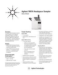
Figure 1 shows a diagram of the Agilent 6100 Series 

Quadrupole LC/MS systems. The ionization of a sample 

occurs at atmospheric pressure in the ion source that is 

shown on the left. The Agilent 6100 Series Quadrupole 

LC/MS systems are compatible with a number of Agilent 

atmospheric pressure ionization (API) sources. 

HPLC inlet 

nebulizer 

capillary 

ion optics 

quadrupole 

mass filter 

detector 

ion 

source 

Figure 1 

rough 

pump 

split-flow 

turbo pump 

Block diagram for an Agilent quadrupole LC/MS system 

API – atmospheric pressure 

ionization 

A common atmospheric sampling interface introduces ions 

from these ionization sources into the vacuum system of the 

mass spectrometer. Various ion- optic elements focus and 

guide the ions through a series of vacuum stages until they 

reach the quadrupole mass analyzer, which separates the 

ions. The ions then travel to the detector, where they are 

recorded as signals. 


Overview of Hardware and Software 1 

Details 

Details 

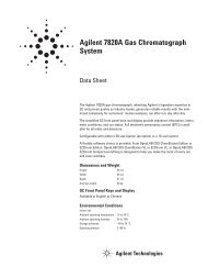
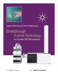
Figure 2 and Figure 3 show more detailed schematics of the 

ion paths in the Agilent 6100 Series Quadrupole LC/MS 

systems. After the API source forms ions, the ion- optic 

elements in the ion transport and focusing region of the 

system direct the ions toward the quadrupole and the 

detector. During transit, the ions move from atmospheric 

pressure (760 torr) at the source to a vacuum in the 10 -6 

torr range at the quadrupole and detector. 

Vacuum stage: 


nebulizer 

1 2 3 

skimmer 

octopole 

4 

capillary 

3 torr 

5X10 -6 torr 

detector 

Figure 2 

Ion source 

fragmentation 

zone (CID) 

lenses 

quadrupole 

Ion transport and focusing region 

Ion path for Agilent 6130 and 6150 Quadrupole LC/MS systems 



Details 

Vacuum stage: 


nebulizer 

1 2 3 

skimmers 

octopole 

4 

capillary 

2 torr 

6X10 -6 torr 

detector 

Figure 3 

Ion source 

fragmentation 

zone (CID) 

lenses 

quadrupole 

Ion transport and focusing region 

Ion path for Agilent 6120 Quadrupole LC/MS system 

The ion transport and focusing region of the Agilent 6100 

Series Quadrupole LC/MS systems is enclosed in a vacuum 

manifold. The function of the vacuum system is to evacuate 

regions of ion focusing and transport and keep the 

quadrupole at low pressure. 

By autotuning the instrument, you 

automatically set most of the 

voltages for the elements in the ion 

path. See “Preparation of the MS – 

tuning” on page 44. 

Because the nebulizer is at a right angle to the inlet 

capillary, most of the solvent is vented from the spray 

chamber and never reaches the capillary. Only ions, drying 

gas, and a small amount of solvent are transmitted through 

the capillary. 

The following discussion of the ion optics is organized 

according to the stages of the ion path and the vacuum 

stages of the mass spectrometer. 

Ion transport and fragmentation (first vacuum stage) 

Ions produced in the API source are electrostatically drawn 

through a drying gas and then through a heated sampling 

capillary into the first stage of the vacuum system. Near the 



Details 

exit of the capillary is a metal skimmer with a small hole. 

Heavier ions with greater momentum pass through the 

skimmer aperture. Most of the lighter drying gas (nitrogen) 

molecules are deflected by the skimmer and pumped away 

by a rough pump. The ions that pass through the skimmer 

move into the second stage of the vacuum system. 

CID – collision-induced 

dissociation 

The atmospheric pressure ionization techniques are all 

relatively “soft” techniques. They generate primarily: 

• Molecular ions M + or M - 

• Protonated molecules [M + H] + 

• Simple adduct ions [M + Na] + 

• Ions representing simple losses, such as the loss of a 

water molecule [M + H - H 2 O] + 

These types of ions give molecular weight information, but 

you often need complementary structural information. To 

gain structural information, you can fragment the analyte 

ions in the first vacuum stage. To do that, you give them 

extra energy and collide them with neutral molecules in a 

process known as collision- induced dissociation (CID). A 

voltage is applied at the end of the atmospheric sampling 

capillary to add energy to the collisions and create more 

fragmentation. For more information, see “Generation of 

fragment ions: low versus high fragmentor” on page 16. 

Ion transport (second and third vacuum stages) 

An octopole ion guide is a set of 

small parallel metal rods with a 

common open axis through which 

the ions can pass. 

Agilent 6130 and 6150 Quadrupole LC/MS systems In the 

second vacuum stage, the ions are immediately focused by 

an octopole ion guide that traverses two vacuum stages. The 

ions pass through the octopole ion guide because of the 

momentum they received from being drawn from 

atmospheric pressure through the sampling capillary. 

Radio- frequency voltage applied to the octopole rods repels 

ions above a particular mass range to the open center of the 

rod set. The ions exit this ion guide and then pass through 

two focusing lenses into the fourth stage of the vacuum 

system. 



Details 

Agilent 6120 Quadrupole LC/MS system In the second vacuum 

stage, the ions are transported between skimmer 1 and 

skimmer 2. They then enter the third vacuum stage, where 

they pass through the octopole ion guide. The ions exit this 

ion guide and then pass through two focusing lenses into the 

fourth stage of the vacuum system. 

Ion separation and detection (fourth vacuum stage) 

m/z – mass/charge ratio 

In the fourth vacuum stage, the quadrupole mass analyzer 

separates the ions by mass- to- charge ratio. An electron 

multiplier then detects the ions. 

The quadrupole mass analyzer (Figure 4) consists of four 

parallel rods to which specific direct- current (DC) and 

radio- frequency (RF) voltages are applied. The analyte ions 

are directed down the center of the rods. Voltages applied to 

the rods generate electromagnetic fields. These fields 

determine which mass- to- charge ratio of ions can pass 

through the filter at a given time. The ions that pass through 

are focused on the detector. 

To detector 

From ion 

source 

Figure 4 

Quadrupole mass analyzer 



Types of data you can acquire 

Types of data you can acquire 

Scan versus selected ion monitoring (SIM) 

You set up a scan or SIM analysis 

in the Method and Run Control 

view, described in Chapter 3. 

As shown in Figure 5, quadrupole mass analyzers can 

operate in two modes. To get the most from your analysis, it 

is important to pick the appropriate mode. The discussion 

below will help you choose. 

scan 

m/z 

1 scan 

abundance 

mass range 

time 

m/z 

SIM 

1 scan 

discrete masses 

m/z 

abundance 

time 

m/z 

Figure 5 

A quadrupole mass analyzer can operate in either scan mode 

or selected ion monitoring (SIM) mode 

Scan mode 

In scan mode, a range of m/z values are analyzed, for 

example, m/z 200 to 1000. The quadrupole sequentially 

filters one mass after another, with an entire scan typically 

taking about a second. (The exact time depends on mass 

range and scan speed.) The MS firmware steps the 

quadrupole through increasing DC and RF voltages, which 

sequentially filters the corresponding m/z values across a 

mass spectrum. 



Generation of fragment ions: low versus high fragmentor 

A full scan analysis is useful because it shows all of the ions 

in a given mass range that are present in the ion source. 

Because it provides a complete picture of all the ionized 

compounds that occur above the detection limit in the 

chosen mass range, a full scan analysis is often used for 

sample characterization, structural elucidation, and impurity 

analysis. It is also the starting point for development of 

methods for SIM data acquisition (discussed next). 

Selected ion monitoring (SIM) mode 

To obtain the best sensitivity, the quadrupole is operated in 

SIM mode. In SIM mode, the quadrupole analyzes the signals 

of only a few specific m/z values. The required RF/DC 

voltages are set to filter one mass at a time. Rather than 

stepping through all the m/z values in a given mass range, 

the quadrupole steps only among the values that the analyst 

chooses. Because the quadrupole spends more time sampling 

each of these chosen m/z values, the system can detect lower 

levels of sample. 

SIM mode is significantly more sensitive than scan mode but 

provides information about fewer ions. Scan mode is 

typically used for qualitative analyses or for quantitation 

when analyte masses are not known in advance. SIM mode 

is used for quantitation and monitoring of target compounds. 


When you set up a method for data 

acquisition, you can control the 

amount of fragmentation with the 

fragmentor setting. You set up a 

method in the Method and Run 

Control view, described in 

Chapter 3. 

Fragment ions, also known as product ions, are formed by 

breaking apart precursor ions. On the Agilent 6100 Series 

Quadrupole LC/MS systems, the fragmentation region is 

between the capillary exit and the skimmer, where the gas 

pressure is about 2 to 3 torr. Depending on the voltage in 

this region, precursor ions may pass through unchanged or 

they may be fragmented. 




When a lower voltage is applied across this region, the ions 

pass through unchanged. Even if these ions collide with the 

gas molecules in this region, they usually do not have 

enough energy to fragment. (See Figure 6.) 

279.1 

300000 

O 

S 

NH 

CH 3 

N CH 3 

350000 

O 

N 

[M + H] + 

250000 

200000 

H 2 N 

150000 

100000 

50000 

280.0 

281.0 

301.0 

[M + Na] + 

0 

100 200 300 

m/z 

Figure 6 

Mass spectrum of sulfamethazine – low fragmentor 




124.1 

m/z186 

m/z156 

O 

N 

80000 

60000 [M + H] + [M + Na] + 

156.1 

186.0 

279.1 

H 2 N 

O 

S 

NH 

m/z124 

CH 3 

N CH 3 

m/z108 

m/z213 

40000 

301.0 

108.2 

20000 

107.1 

125.1 

157.1 

187.0 

213.2 

280.1 

323.0 

0 

100 200 300 

m/z 

Figure 7 

Mass spectrum of sulfamethazine – high fragmentor 

FIA – flow injection analysis 

If the voltage is increased, the ions have more translational 

energy. Then, if the ions collide with gas molecules, the 

collisions convert the translational energy into molecular 

vibrations that can cause the ions to fragment. This is called 

collision- induced dissociation (CID). Figure 7 shows an 

example. Even though this fragmentation does not occur 

where the ions are formed at atmospheric pressure, it is a 

tradition to call this type of fragmentation “in- source CID.” 

The ions from molecular fragments are used for structural 

determination or confirmation of the presence of a 

particular chemical species. 

It is possible to produce both molecular ions and fragment 

ions within the same spectrum by using an intermediate 

fragmentation voltage. 

The ideal fragmentation voltage depends on the structure of 

the compound and the needs of the analysis. For target 

compound analysis, it is good practice to determine in 

advance the compound’s response to fragmentor setting. The 

fastest way to accomplish this is with a flow injection 

analysis (FIA) series. An FIA series allows you to inject the 



Positive versus negative ions 

compound multiple times within the same run, and to vary 

the fragmentor setting in different time windows. From the 

resulting data, you can judge the best fragmentor setting. For 

more information on FIA, see “Flow injection analysis” on 

page 71. 

Positive versus negative ions 

You set the ion polarity when you 

set up a method in the Method and 

Run Control view, described in 

Chapter 3. 

Atmospheric pressure ionization techniques can produce 

both positive and negative ions. For any given analysis, the 

predominant ion type depends on the chemical structure of 

the analyte and (particularly for electrospray ionization) the 

pH of the solution. While either or both ion types may be 

present in the ion source, the polarity of the ion optics in 

the ion transport and focusing region determines which ion 

type is detected. 

Analyses of positive and negative ions require different 

settings for the ion optics. The software- controlled autotune 

process optimizes the settings for both positive and negative 

ions, and stores them in a single tune file. During data 

acquisition, the software accesses the tune file for the 

appropriate settings. 

Multiple signal acquisition 

You establish the conditions for 

multiple signal acquisition in the 

Method and Run Control view, 

described in Chapter 3. 

The Agilent 6120, 6130 and 6150 LC/MS models allow you to 

acquire multiple types of data during a single analysis. 

Within a single analytical run, you can choose alternating 

positive and negative ionization; alternating high and low 

fragmentor settings; and alternating scan and SIM modes. 

Because optimum MS conditions vary from compound to 

compound, this multisignal capability enables you to analyze 

more compounds, with greater sensitivity, within a single 

run. 




Polarity switching 

The Agilent 6120, 6130 and 6150 LC/MS models allow you to 

switch from scan to scan between analysis of positive ions 

and analysis of negative ions. To switch polarities very 

quickly, these models incorporate fast- switching power 

supplies for the API source, the lens system, the quadrupole, 

and the detector. The ability to switch polarities on the 

chromatographic time scale is very useful for analysis of 

complete unknowns because it obviates the need to run the 

sample twice to detect both types of ions. 

Alternating high/low fragmentor 

With the Agilent 6120, 6130 and 6150 LC/MS models, you 

can also alternate from scan to scan between high and low 

fragmentation voltages. This capability allows you to acquire 

scans at low fragmentor settings for molecular weight 

information, and high fragmentor settings for structural 

information. 

Alternating SIM/scan 

Many analyses require use of SIM mode to monitor and/or 

quantitate target compounds at very low levels. Sometimes it 

is also desirable to characterize the other sample 

components with a scan analysis. The Agilent 6120, 6130 

and 6150 LC/MS models allow you to alternate between SIM 

and scan modes, so you can accomplish both goals in a 

single analysis. 

Putting it all together 

The 6120, 6130 and 6150 LC/MS models can cycle through 

four different user- selected acquisition modes on a 

scan- by- scan basis within a single run. For example, you can 

set up a single run to do the following: 

• Positive ion scan with low fragmentor voltage 

• Positive ion scan with high fragmentor voltage 

• Negative ion scan with low fragmentor voltage 

• Negative ion scan with high fragmentor voltage 




Such an analysis is ideal for a mixture of compounds where 

some respond better in positive mode and some respond 

better in negative mode, and where you need both molecular 

ions and fragment ions. 

The time required for one cycle varies depending on the 

number of modes chosen, the scan range, and the interscan 

delay required for the switching. For separations with 

narrow chromatographic peaks, it is important to ensure 

that total cycle time is short enough that the instrument 

makes sufficient measurements across the peak. 



Ion sources 

Ion sources 

The Agilent 6100 Series Quadrupole LC/MS systems operate 

with the following interchangeable atmospheric pressure 

ionization (API) sources: 

• ESI (electrospray ionization) 

• ESI with Agilent Jet Stream technology (6150 only) 

• APCI (atmospheric pressure chemical ionization) 

• APPI (atmospheric pressure photoionization) 

• MMI (multimode ionization) 

NOTE 

The sources that are used on the 6100 Series LC/MS systems are the 

B-type sources. The 6100 Series LC/MS systems are not compatible with 

the A-type sources that were used on previous Agilent LC/MS models. 

Electrospray ionization (ESI) 

You control the spray chamber 

parameters (nebulizer pressure, 

drying gas flow and temperature, 

and capillary voltage) when you set 

up a method in the Method and 

Run Control view, described in 

Chapter 3. 

Electrospray ionization relies in part on chemistry to 

generate analyte ions in solution before the analyte reaches 

the mass spectrometer. As shown in Figure 8, the LC eluent 

is sprayed (nebulized) into a spray chamber at atmospheric 

pressure in the presence of a strong electrostatic field and 

heated drying gas. The electrostatic field occurs between the 

nebulizer, which is at ground in the Agilent design, and the 

capillary, which is at high voltage. 

The spray occurs at right angles to the capillary. This 

patented Agilent design reduces background noise from 

droplets, increases sensitivity, and keeps the capillary 

cleaner for a longer period of time. 





nebulizer 

capillary 

solvent 

spray 

heated drying gas 

Figure 8 

Electrospray ion source 

Electrospray ionization (ESI) consists of four steps: 

1 Formation of ions 

2 Nebulization 

3 Desolvation 

4 Ion evaporation 

Formation of ions 

Ion formation in API- electrospray occurs through more than 

one mechanism. If the chemistry of analyte, solvents, and 

buffers is correct, ions are generated in solution before 

nebulization. This results in high analyte ion concentration 

and good API- electrospray sensitivity. 




Preformed ions are not always required for ESI. Some 

compounds that do not ionize in solution can still be 

analyzed. The process of nebulization, desolvation, and ion 

evaporation creates a strong electrical charge on the surface 

of the spray droplets. This can induce ionization in analyte 

molecules at the surface of the droplets. 

Nebulization 

Nebulization (aerosol generation) takes the sample solution 

through these steps: 

a 

b 

c 

d 

e 

Sample solution enters the spray chamber through a 

grounded needle called a nebulizer. 

For high- flow electrospray, nebulizing gas enters the 

spray chamber concentrically through a tube that 

surrounds the needle. 

The combination of strong shear forces generated by 

the nebulizing gas and the strong voltage (2–6 kV) in 

the spray chamber draws out the sample solution and 

breaks it into droplets. 

As the droplets disperse, ions of one polarity 

preferentially migrate to the droplet surface due to 

electrostatic forces. 

As a result, the sample is simultaneously charged and 

dispersed into a fine spray of charged droplets, hence 

the name electrospray. 

Because the sample solution is not heated when the aerosol 

is created, ESI does not thermally decompose most analytes. 

Desolvation and ion evaporation 

Before the ions can be mass analyzed, solvent must be 

removed to yield a bare ion. 

A counter- current of neutral, heated drying gas, typically 

nitrogen, evaporates the solvent, decreasing the droplet 

diameter and forcing the predominantly like surface- charges 

closer together (see Figure 9). 




evaporation 

analyte ion ejected 

+ 

+ + + + 

+ - - + +++ 

++ 

- - - ++++ - - - 

+ ++ - 

+ ++ 

+ + 

+ - +++ - - 

- 

+ +++ 

+ 

+ + + 

+ - + 

- 

Figure 9 

Desorption of ions from solution 

Coulomb repulsion – repulsion 

between charged species of the 

same sign 

When the force of the Coulomb repulsion equals that of the 

surface tension of the droplet, the droplet explodes, 

producing smaller charged droplets that are subject to 

further evaporation. This process repeats itself, and droplets 

with a high density of surface- charges are formed. When 

charge density reaches approximately 10 8 V/cm 3 , ion 

evaporation occurs (direct ejection of bare ions from the 

droplet surface). These ions are attracted to and pass 

through a capillary sampling orifice into the ion optics and 

mass analyzer. 

The importance of solution chemistry 

The choice of solvents and buffers is a key to successful 

ionization with electrospray. Solvents like methanol that have 

lower heat capacity, surface tension, and dielectric constant, 

promote nebulization and desolvation. For best results in 

electrospray mode: 

• Adjust solvent pH according to the polarity of ions 

desired and the pH of the sample. 

• To enhance ion desorption, use solvents that have low 

heats of vaporization and low surface tensions. 

• Select solvents that do not neutralize ions through 

gas- phase reactions such as proton transfer or ion pair 

reactions. 

• To reduce the buildup of salts in the ion source, select 

more volatile buffers. 




Multiple charging 

Electrospray is especially useful for analyzing large 

biomolecules such as proteins, peptides, and 

oligonucleotides, but can also analyze smaller molecules like 

drugs and environmental contaminants. Large molecules 

often acquire more than one charge. Because of this multiple 

charging, you can use electrospray to analyze molecules as 

large as 150,000 u even though the mass range (or more 

accurately mass- to- charge range) for a typical quadrupole 

LC/MS instrument is around 3000 m/z. For example: 

The optional Agilent LC/MSD 

Deconvolution & Bioanalysis 

Software performs the calculations 

to accomplish deconvolution. 

100,000 u / 10 z = 1,000 m/z 

When a large molecule acquires many charges, a 

mathematical process called deconvolution is used to 

determine the actual molecular weight of the analyte. 

Agilent Jet Stream Technology 

The Agilent Jet Stream technology is supported on the 

Agilent 6150 Quadrupole LC/MS system. 

Agilent Jet Stream Technology enhances analyte desolvation 

by collimating the nebulizer spray and creating a 

dramatically “brighter signal.” The addition of a collinear, 

concentric, superheated nitrogen sheath gas (Figure 10) to 

the inlet assembly significantly improves ion drying from the 

electrospray plume and leads to increased mass spectrometer 

signal to noise allowing the triple quadrupole to surpass the 

femtogram limit of detection. The Agilent Jet Stream 

Technology is patent pending. 




Figure 10 

Electrospray Ion Source with Agilent Jet Stream Technology 

Agilent Jet Stream thermal gradient focusing consists of a 

superheated nitrogen sheath gas that is introduced collinear 

and concentric to the pneumatically assisted electrospray. 

Thermal energy from the superheated nitrogen sheath gas is 

focused to the nebulizer spray producing the most efficient 

desolvation and ion generation possible. The enhanced 

molecular ion desolvation results in more ions entering the 

sampling capillary as shown in Figure 10 and concomitant 

improved signal to noise. Parameters for the Agilent Jet 

Stream Technology are the superheated nitrogen sheath gas 

temperature and flow rate and the nozzle voltage. 

The capillary in the 6460A is a resistive capillary that 

improves ion transmission and allows virtually instantaneous 

polarity switching. It is the same, proven capillary that is 

used in the fast polarity switching version of Agilent's single 

quadrupole product. 



Atmospheric pressure chemical ionization (APCI) 


APCI is a gas- phase chemical ionization process. The APCI 

technique passes LC eluent through a nebulizing needle, 

which creates a fine spray. The spray is passed through a 

heated ceramic tube, where the droplets are fully vaporized 

(Figure 11). 

The resulting gas/vapor mixture is then passed over a 

corona discharge needle, where the solvent vapor is ionized 

to create reagent gas ions. These ions in turn ionize the 

sample molecules via a chemical ionization process. The 

sample ions are then introduced into the capillary. 


nebulizer (sprayer) 

vaporizer 

(heater) 

drying gas 

+ ++ 

+ + + + 

corona 

discharge 

needle 

Figure 11 

capillary 

Atmospheric pressure chemical ionization (APCI) source 

APCI requires that the analyte be in the gas phase for 

ionization to occur. To vaporize the solvent and analyte, the 

APCI source is typically operated at vaporizer temperatures 

of 400 to 500 °C. 




APCI is applicable across a wide range of molecular 

polarities. It rarely results in multiple charging, so it is 

typically used for molecules less than 1,500 u. Because of 

this molecular weight limitation and use of high- temperature 

vaporization, APCI is less well- suited than electrospray for 

analysis of large biomolecules that may be thermally 

unstable. APCI is well suited for ionization of the less polar 

compounds that are typically analyzed by normal- phase 

chromatography. 



Atmospheric pressure photoionization (APPI) 

Atmospheric pressure photoionization (APPI) 

With the APPI technique, LC eluent passes through a 

nebulizing needle to create a fine spray. This spray is passed 

through a heated ceramic tube, where the droplets are fully 

vaporized. The resulting gas/vapor mixture passes through 

the photon beam of a krypton lamp to ionize the sample 

molecules (Figure 12). The sample ions are then introduced 

into the capillary. 

APPI and APCI are similar, with APPI substituting a lamp 

for the corona needle for ionization. APPI often also uses an 

additional solvent or mobile phase modifier, called a 

“dopant”, to assist with the photoionization process. 

APPI is applicable to many of the same compounds that are 

typically analyzed by APCI. APPI has proven particularly 

valuable for analysis of nonpolar compounds. 


nebulizer (sprayer) 

vaporizer 

(heater) 

drying gas 

h 

+ ++ 

+ + + + 

UV lamp 

Figure 12 

capillary 

Atmospheric pressure photoionization (APPI) source 



Multimode ionization (MMI) 


The multimode source is an ion source that can operate in 

three different modes—APCI, ESI or simultaneous APCI/ESI. 

The multimode source incorporates two electrically 

separated, optimized zones—one for ESI and one for APCI. 

During simultaneous APCI/ESI, ions from both ionization 

modes enter the capillary and are analyzed simultaneously 

by the mass spectrometer. 


nebulizer 

APCI 

zone 

corona 

discharge 

needle 

ESI zone 

thermal container 

capillary 

drying gas 

Figure 13 

Multimode source 

Multimode ionization (MMI) is useful for screening of 

unknowns, or whenever samples contain a mixture of 

compounds where some respond by ESI and some respond 

by APCI. In these cases, the multimode source obviates the 

need to run the samples twice to accomplish a complete 

analysis. 




Unlike the APCI and APPI sources where the temperature of 

the vaporizer is monitored, in the multimode source the 

actual vapor temperature is monitored. As a result, the 

vaporizer is typically set to between 200 and 250 °C. 



Introduction to ChemStation software 

Introduction to ChemStation software 

Overview 

ChemStation software for the Agilent 6100 Series 

Quadrupole LC/MS systems is organized into views. Each 

view allows you to do a specific set of tasks. The menus and 

toolbars change with each view. 

Figure 14 

These buttons allow you to switch among the six ChemStation 

views 

For more information about the 

Method and Run Control view, see 

Chapter 3. 

The following summarizes the ChemStation views and their 

functionality: 

Method and Run Control 

• Set up methods 

• Change setpoints for the Agilent 1100 Series LC or 

Agilent 1200 Series LC modules, including the Chip 

Cube 

• Change setpoints for the Agilent 6100 Series 

Quadrupole LC/MS systems 

• Change setpoints for the Agilent API sources 

• Run single samples 

• Run automated sequences 

• Run an FIA series 



Overview 


Data Analysis view, see Chapter 4. 


Report Layout view, see Chapter 5. 


Verification view, see Chapter 6. 


Diagnosis view, see Chapter 7. 


MSD Tune view, see Chapter 2. 

• View data in real time, as it is acquired 

Data Analysis 

• View chromatograms and spectra from the MS and UV 

detectors 

• Integrate chromatographic peaks 

• Perform quantitation 

• Check peak purity 

• Deconvolute multiply charged spectra 

• Generate reports 

• Reprocess data from sequences 

Report Layout 

• Design custom report templates 

Verification (OQ/PV) 

• Verify system performance 

Diagnosis 

• Learn possible causes of instrument problems 

• Run tests to diagnose instrument problems 

• Receive notification when it is time to perform system 

maintenance 

• Pump down and vent the system 

MSD Tune 

• Optimize and calibrate the MS 



Reviewing data remotely 


There are two ways to set up a computer so you can review 

ChemStation data remotely. 

One way is to install a Data Analysis- only version of 

ChemStation software on the remote computer. This 

installation provides the same Data Analysis functionality 

that you have on the ChemStation that controls your Agilent 

6100 Series LC/MS system. It is ideal if you need full 

features for in- depth data analysis. 

Another way is to install the Analytical Studio Reviewer on 

the remote computer. Analytical Studio Reviewer lets you 

easily review ChemStation LC and LC/MS data files, but the 

functionality is different than with the full ChemStation 

Data Analysis. The Analytical Studio Reviewer software is 

ideal for synthetic chemists and others who use the LC/MS 

system for “walk- up” analysis. 







2 

Instrument Preparation 

Preparation of the LC system 38 

Purpose 38 

Summary of procedures 38 

Setting parameters for LC modules 40 

Column conditioning and equilibration 41 

Monitoring the stability of flow and pressure 43 

Preparation of the MS – tuning 44 

Overview 44 

Ways to tune 46 

When to tune – Check Tune 47 

Autotune 49 

Manual tuning 51 

Tune reports 53 

Gain calibration 55 

In this chapter, you learn the concepts that help you prepare 

the instrument for an analysis. This chapter assumes that 

the hardware and software are installed, the instrument is 

configured and the performance verified. If this has not been 

completed, see the Agilent 6100 Series Single Quad LC/MS 

System Installation Guide. 


37


Preparation of the LC system 

Preparation of the LC system 

Purpose 

To achieve good sensitivity, it is important to properly 

prepare the LC and column prior to an LC/MS analysis. 

For best signal- to- noise, the entire LC system must be free 

of contamination from salts (such as nonvolatile buffers) and 

unwanted organic compounds. Some contaminants that are 

not bothersome for a UV detector can cause problems for 

the MS. Contaminants may cause ion suppression and/or 

high background, and these problems can seriously degrade 

sensitivity. 

To achieve a smooth baseline with little noise, the LC flow 

must also be very stable. 

Summary of procedures 

The exact LC preparation steps depend on how the LC was 

used previously and the type of analysis to be performed. 

The following provides guidelines: 

Typical preparation 

Before beginning an analysis, the entire LC path should be 

contaminant- free and the flow should be stable. Usually, you 

can accomplish these goals by doing the following: 

1 Purge the pump to remove air bubbles. Purge each 

channel that you plan to use. 

For instructions to purge the pump, search the online 

Help for the keyword “purge” and scroll down the list of 

topics until you see entries that begin with the word 

“purge.” 

2 Condition the column to remove impurities or residual 

sample. 


Instrument Preparation 2 

Summary of procedures 

For more information, see “Column conditioning and 

equilibration” on page 41. 

3 Equilibrate the column at the initial mobile phase 

composition. 

For more information, see “Column conditioning and 

equilibration” on page 41. 

4 Ensure that the system flow and pressure are stable. 

For more information, see “Monitoring the stability of 

flow and pressure” on page 43. 

More extensive preparation 

While the four- step procedure that is outlined above works 

well on a day-to-day basis, more extensive LC/column 

flushing may be necessary if any of the following are true: 

• You have not used this LC for MS. 

• The column is new. 

• You are changing to a different mobile phase composition. 

• The LC was used to analyze dirty samples. 

• The next analysis requires ultimate sensitivity. 

A protocol for more thorough LC cleaning is given in the 

Agilent 6100 Single Quad System Installation Guide. See 

the section on conditioning the LC in the chapter on system 

verification. 

When you flush the LC, remember to flush all channels that 

you plan to use. Also, flush the injector by making several 

injections of the same solvent(s) that you use to flush the 

system. 



Setting parameters for LC modules 

Setting parameters for LC modules 

You set up the LC modules in the Method and Run Control 

view. Within the system diagram, click each module to set 

parameters. 

Injection 

Pump 

Diode-array detector 

Solvent bottles Column thermostat, 

Column switching valve 

Mass spectrometer 

Figure 15 

Example system diagram (yours may be different) 

To access help for any system module, click Help on the 

module context menu. To access help for a given dialog box, 

click the Help button on the dialog box. 

To set module control parameters 

Alternate 

method 

This procedure uses the pump module as an example. 

1 Click More Pump > Control HPLC Pump on the 

Instrument menu to open the Pump Control dialog box. 

2 Set desired control parameters and click OK. 

Select the desired control parameter such as Standby from 

the Pump context menu. 



Column conditioning and equilibration 

To set module setpoint parameters 

This procedure uses the binary pump module as an example. 

1 Click Set up Instrument Method on the Instrument menu 

to open the Setup Method dialog box. 

2 Click the BinPump tab. 

3 Set desired setpoints and click OK. 

To access other instrument parameters 

1 Click to open the Instrument menu. 

2 Click the desired command such as Select Injection 

Source, Columns, or Instrument Configuration. 


There are several ways to set parameters to condition and 

equilibrate a column. 

Conditioning 

Column conditioning eliminates any previously separated 

compounds or impurities from the column, particularly after 

runs with solvent of a single composition (isocratic runs). 

There are a number of ways to condition a column before a 

sample run. One way is to pump the organic solvent that 

you intend to use (100% solvent B) through the column for a 

period of time. Another way is to run the gradient that you 

intend to use, then extend the time at the final composition 

until no further peaks elute. 

When a column is new, “conditioning” may include injecting 

a few samples or high- level standards until peak area and 

retention time are stable. 




Equilibration 

Column equilibration returns column characteristics to their 

initial state after a gradient run. To equilibrate a column 

before a sample run, you pass the solvent of initial 

composition through the column for a period of time. 


You set up a method or sequence in 

the Method and Run Control view, 

described in Chapter 3. 

You can condition and equilibrate a column in one of three 

ways with ChemStation software. 

• Interactively 

You set the pump to the solvent composition for the end 

of the run and higher- than- normal flow rates. You can 

then immediately apply these setpoints to the pump. After 

you pump about three column- volumes of solvent, then 

set the pump to the solvent composition and flow rate for 

the beginning of the run. With this procedure, you do not 

store a data file. 

If you use this procedure, you can tune the MS while you 

condition and equilibrate the column. When you tune the 

MS, the MS stream selection valve automatically diverts 

the LC effluent to waste. For information on tuning, see 

“Preparation of the MS – tuning” on page 44. 

• With a method in an interactive run 

You set up a method for your analysis and then run a 

solvent blank. The run uses the method stop time. You 

can also use a post- run time within the method to 

equilibrate the column. 

With this procedure, you store a data file. 

• With a sequence 

You set up a method for your analysis and then set up a 

solvent blank as the first run in a sequence. The method 

includes a post- run time to equilibrate the column. 

With this procedure, you store a data file. 



Monitoring the stability of flow and pressure 

Monitoring the stability of flow and pressure 

Chapter 3 provides more 

information about online signals, 

which are also called online plots. 

The LC solvent flow and the system backpressure must be 

stable to ensure a quiet baseline and best results for 

API- MS. The best time to monitor the stability of flow and 

pressure is after you have equilibrated the column, and 

before you start the analysis. 

You can measure stability with ChemStation software. To do 

this, you set up an isocratic method with the same solvent 

composition as the initial composition you intend to use for 

your analysis. During the run, you monitor the online signals 

for flow and pressure. 



Preparation of the MS – tuning 

Preparation of the MS – tuning 

Overview 

Use the MSD Tune view for all 

tasks that relate to tuning. 

Tuning is the process of adjusting MS parameters to 

generate high quality, accurate mass spectra. During tuning, 

the MS is optimized to: 

• Maximize sensitivity 

• Maintain acceptable resolution 

• Ensure accurate mass assignments 

Parameters that are adjusted 

The Agilent 6100 Series Quadrupole LC/MS systems have 

two sets of parameters that can be adjusted. One set of 

parameters is associated with the formation of ions. These 

parameters control the spray chamber (for example, 

electrospray or APCI) and fragmentor. The other set of 

parameters is associated with the transmission, filtering, and 

detection of ions. These parameters control the skimmer, 

octopole, lenses, quadrupole mass filter, and high- energy 

dynode (HED) electron multiplier (detector). 

Tuning is primarily concerned with finding the correct 

settings for the parameters that control the transmission, 

filtering, and detection of ions. It is accomplished by 

introducing a calibrant into the MS and generating ions. 

Using these ions, the tune parameters are then adjusted to 

achieve sensitivity, resolution, and mass assignment goals. 

With a few exceptions, the parameters that control ion 

formation are not adjusted. They are set to fixed values 

known to be good for generating ions from the calibrant 

solution. 



Overview 

Tune files and reports 

The product of tuning is a tune file (actually a directory) 

that contains parameter settings for both positive and 

negative ionization. When data acquisition uses a tune file, 

the settings appropriate for the ion polarity specified by the 

data acquisition method are loaded automatically. 

Autotune, the automated tuning program, also generates a 

report. See page 53. 

Use of tune files during data acquisition 

During data acquisition, the parameters associated with ion 

formation are controlled by the data acquisition method. The 

parameters associated with ion transmission are controlled 

by the tune file assigned to the data acquisition method. 



Ways to tune 

Ways to tune 

Access this functionality via the 

Tune menu in the MSD Tune view. 

NOTE 

ChemStation software provides the following two ways to 

tune the MS: 

• Autotune is an automated tuning program that tunes the 

MS for good performance over the entire mass range. It 

uses known compounds in a standard calibration mixture 

that is introduced via the Calibrant Delivery System 

(CDS). This is the tuning method that you use in most 

cases. 

• Manual Tune allows you to tune the MS by adjusting one 

parameter at a time until you achieve the desired 

performance. Manual tuning is most often used when you 

need maximum sensitivity, when your analysis targets a 

restricted mass range, or when you need a tuning 

compound other than the standard calibrants. 

In addition, a Check Tune program allows you to determine 

whether you need to tune. 

Check Tune, Autotune, and Manual Tune are discussed in 

more detail in the next sections. 

Frequent tuning is not required for normal operation. Once tuned, the 

LC/MS is very stable. Tuning is generally not needed more often than 

monthly, or at most weekly. If you suspect problems related to tuning, use 

the Check Tune program to confirm that the MS is out of adjustment 

before you retune it. 

CAUTION 

Wait at least four hours after pump-down before tuning or operating 

your Agilent 6100 Series LC/MS system. Ceramic components in the 

quadrupole mass filter can absorb moisture from the air. Tuning or 

acquiring data too soon may result in arcing. Further, it takes the 

analyzer at least nine hours to reach thermal equilibrium. Tune files 

created or data acquired before the MS is at thermal equilibrium may 

have incorrect mass assignments and other inaccuracies. 



When to tune – Check Tune 


Check Tune allows you to quickly determine whether the MS 

is correctly tuned without performing a complete autotune. 

It performs a single profile scan of the tune masses and 

compares the peak widths and mass axes with target values. 

If the values obtained by Check Tune are within acceptable 

ranges, the tune report indicates that Check Tune passes. 

(See Figure 16 on page 48.) If the values are outside of 

acceptable ranges, Check Tune suggests that you adjust peak 

widths or calibrate the mass axis. 

A third parameter, gain, may be added to the parameters 

checked by Check Tune. If so, Check Tune compares the 

current gain value with the gain value from the most recent 

autotune. For a discussion of gain, see page 55. 




All masses pass the 

mass axis and peak 

width tests 

Figure 16 

Check Tune report 



Autotune 

Autotune 

Autotune is a program that adjusts the MS for good 

performance over the entire mass range. 

Autotune files 

A tune file, ATUNES.TUN is provided as a starting point for 

autotune. 

The results of autotune are saved to the current autotune 

file. This makes autotune faster because each autotune 

begins from the most recent good tune parameters. This 

means, however, that previous tune values are lost. You may 

want to occasionally save the autotune file to a different file 

name before using autotune. 

A single autotune file contains the results of both positive 

ionization and negative ionization autotunes. 

Autotune polarity and scan speed 

You have six choices for running an autotune: 

• Dual Polarity 

• Positive Polarity 

• Negative Polarity 

• Dual Polarity Fast Scan 

• Positive Polarity Fast Scan 

• Negative Polarity Fast Scan 

The Dual Polarity modes perform an autotune for both 

positive ionization and negative ionization. Positive Polarity 

and Negative Polarity modes perform autotunes only for the 

specified polarity. 

Gain checking in autotune 

Gain checking occurs only in the positive polarity autotune 

or the positive portion of a dual polarity autotune. For more 

information on gain checking, see “Gain calibration” on 

page 55. 



Autotune 

Spray chamber parameters 

Autotune adjusts the parameters that affect ion transmission. 

The spray chamber parameters, which affect ion formation, 

are not adjusted by autotune. They are set to default values 

known to be good for generating ions of the calibrant 

solution. 

Because there may be slight variations from spray chamber 

to spray chamber, the default parameters may not be 

optimum for a particular spray chamber. Changes such as 

adjustment of the nebulizer and normal aging of the LC/MS 

system components can also result in a system where the 

default values are not optimum. Therefore, it is possible to 

manually set the spray chamber parameters. Typically, this is 

necessary only when the instrument fails autotune or when 

the results of autotune show a significant decrease in system 

performance. Be aware that other factors can also decrease 

system performance. 



Manual tuning 

Manual tuning 

The autotune program adjusts the MS for good performance 

over the entire mass range, and this tune program is 

sufficient for most applications. There are times, however, 

when it is advantageous to tune the MS manually. These 

include: 

• When you want to achieve maximum sensitivity by 

sacrificing some resolution 

• When you want to tune specifically for the very low end 

of the mass range (< 150 u) 

• When you want to tune with a compound other than the 

standard calibrants. 

CAUTION 

The calibrant delivery system (CDS) is designed specifically for precise 

delivery of the Agilent calibrants in a 90:10 acetonitrile:water solvent 

mix. Other solvents and mixes may have different flow rates, which 

may not be optimum for tuning. Further, the O-ring seals in the CDS are 

ethylene-propylene. They can be damaged by aliphatic, aromatic, or 

halogenated hydrocarbons. Never use these types of solvents in the 

CDS. We recommend delivering non-standard calibrants through the 

LC. 

Tips for manual tuning 

Ionization 

modes 

Polarity 

Separate tuning is not required for electrospray, APCI/APPI 

and multimode- ESI+APCI. Tuning involves adjusting the 

parameters that control the transmission of ions. It does not 

matter how those ions are generated. A tune file created in 

electrospray mode often will provide good results for 

APCI/APPI samples. The reverse is also true. 

Separate tuning is required for positive and negative 

ionization. The MS must, at some time, be tuned twice — 

once with positive ions and once with negative ions. The two 

tunes can be stored under the same tune file name. Positive 

ion and negative ion settings can be updated separately. 



Manual tuning 

Mass range 

Tuning is almost always done over the entire mass range. 

The exception is if all the ions of interest are smaller than 

approximately 150 u. Correct manual tuning over a reduced 

mass range can improve transmission and detection of these 

very low mass ions. 

Steps to manual tune 

The online Help includes step- by- step instructions for 

manual tuning. The instructions assume the use of one of 

the standard calibrants and tuning over the entire mass 

range, but they can be altered for non- standard calibrants or 

narrower mass ranges. 

To access the manual tuning instructions: 

1 Open the online Help. 

2 Click to expand “How to Work with Your ChemStation.” 

3 Click to expand “Basic Tasks.” 

4 Click to expand “Method and Run Control.” 

5 Click to expand “MSD Tune.” 

6 Click the link to “Manually Tuning the LC/MSD or 

CE/MSD.” 

7 Scroll down until you see “Steps.” 



Tune reports 

Tune reports 

At the end of every autotune, the system prints a tune 

report. You can also manually print a tune report from the 

File menu. 



Tune reports 

Figure 17 Tune report (page 1 of 4) 



Gain calibration 


Gain calibration sets the electron multiplier voltage in a way 

that simplifies method development and portability. Gain 

calibration is performed automatically during autotune. You 

can also check and adjust the gain calibration during manual 

tune. 

What is gain? 

The HED electron multiplier receives an input current that is 

generated by the ions that strike it, amplifies that current, 

and generates a proportional output current. 

Gain = Output current / input current 

Gain is controlled by the electron multiplier voltage (EMV). 

The higher the EMV, the higher the gain. The relationship 

between EMV and gain is log linear. This linear relationship 

is common for all multipliers. Since the slope of this line is 

constant, to set the gain, the software needs only to adjust 

the intercept. The gain calibration routine simply adjusts the 

value of the intercept for the specific instrument. The 

instrument- specific gain curve coefficients are then stored in 

the MS. 

Gain calibration curve 

A gain calibration curve is generated by taking readings of 

the ion current generated at discreet multiplier settings 

across the range of the multiplier. Separate gain calibration 

curves are generated for positive and negative polarities, 

since the ion current generated in these two modes varies to 

some extent. A gain of 1 is set to be a multiplier value of 

1e6. That is, one electron striking the input side of the 

detector will generate 1e6 on the output side. A gain check 

can be generated on both polarities or on the current 

polarity. 




Gain and method portability 

The use of gain enables the distribution of methods from 

instrument to instrument. In principle, using the same gain 

on two different instruments should result in the same 

signal response, thereby easing method development and 

instrument portability. Because the relationship between 

EMV and gain is log linear, a gain of 2.0 should give twice 

the abundance of a gain of 1.0. 

More gain is not always better 

In general, it is best to run the detector at the lowest gain 

that still produces adequate abundance. High gains increase 

noise as well as signal and often result in poorer 

signal- to- noise ratios. Increasing the gain increases the EMV, 

which shortens the life- span of the electron multiplier. The 

maximum EMV is 3000 eV no matter how high you set the 

gain; a gain of 70 or higher elicits the 3000 eV setting. 

As an electron multiplier ages, it slowly becomes less 

efficient. For a given ion current input, it generates a 

smaller and smaller output current (abundance). Low 

abundance caused by an aging electron multiplier is not 

easily distinguished from low abundance caused by poor ion 

generation or transmission (low ion current input). It may be 

tempting to compensate for poor ion generation or 

transmission by increasing the gain (thereby increasing the 

EMV) even though the electron multiplier is actually 

performing correctly at its previous gain. The increased gain 

will improve abundance, but may decrease the 

signal- to- noise ratio and will shorten the life- span of the 

electron multiplier. 

Check Gain Calibration 

Access this functionality via the 

Tune menu in the MSD Tune view. 

During a Gain Calibration check, a reading of the ion 

current is taken and checked against the current gain 

calibration curve for the current polarity. If it is within 

acceptable limits, no change is made to the curve for that 

polarity. If the reading falls outside the limits, a new gain 

curve is generated. A gain of 1 is set to be a multiplier of 




1e6. That is, one electron striking the input side of the 

detector will generate 1e6 on the output side. If that 

multiplier setting exceeds 2600 volts, which indicates 

decreasing electron multiplier performance or instrument 

performance, you are warned that system maintenance may 

be required. 







3 

Data Acquisition 

Working with methods 60 

Method and Run Control View 60 

Loading, editing, saving and printing methods 62 

More on editing methods 63 

Running samples 66 

Running a single sample 67 

Running a sequence 68 

Flow injection analysis 71 

Monitoring analyses 75 

Online signal plots 75 

Quick method overview 76 

Logbooks 76 

Instrument shutdown 78 

In this chapter, you learn the concepts that help you run 

samples and acquire data. This chapter assumes that the 

hardware and software are installed, the instrument is 

configured and the performance verified. If this has not been 

completed, see the Agilent 6100 Series Single Quad LC/MS 

System Installation Guide. 


59


Working with methods 

Working with methods 

Method and Run Control View 

You set up methods and run analyses from the Method and 

Run Control view, shown in Figure 18. 

ChemStation methods control the instrument during data 

acquisition. The easiest way to prepare a method is to load 

a similar method (or load DEF_LC.M), save it with a new 

name, modify (edit) it, and save it again. Then you can use 

the method to run a single sample or multiple samples via a 

sequence. 

You can also set up a method for flow injection analysis 

(FIA), where you make multiple injections in a single run. 


Data Acquisition 3 

Method and Run Control View 

Tool Set Selection: Sequence 

or Single Sample 

Method 

Sequence 

Top Toolbar 

Status Bar 

Run Control 

File List 

MS, FIA 

System Diagram 

Data 

Analysis 

View Selection 

Disk 

Space 

Online Plot 

Message Line 

Method Overview 

Figure 18 

In this view, you set up methods, establish instrument settings, and inject samples. 

Status and Run Bars: Main Tab 

Right- click the Method icon to see the following commands: 

Run Time Checklist, Method Information, Edit Entire 

Method, Method Audit Trail, Print Method, and Help. 



Loading, editing, saving and printing methods 

Loading, editing, saving and printing methods 

When you need to work with methods, there are several 

ways to access the necessary functionality: 

• Select from the Method menu, which allows you to load, 

edit, save, and print methods. 

• Use the Method icon in the Run Control Bar. 

Right- click the icon to access the context menu. 

• Use the toolbar or method drop- down list. 

When you want to view all the tools for methods (or to 

run a single sample interactively), you first click the icon 

for the Single Sample Toolset, as shown in Figure 19. 

Sequence 

Single sample 

Figure 19 

Toolset selection 

Load a 

Method 

Save 

current 

method 

Select method from 

list of recent methods 

Edit entire 

Method 

Figure 20 

When you click the icon for the Single Sample Toolset, you access tools to work with methods. 

• Use the ChemStation Explorer pane on the left side of the 

Method and Run Control view. 

Click the Method tab at the bottom to display the method 

files. 

Double- click a method to load it. 

Right- click in the white area to view the context menu, 

which contains options such as Load Method. 



More on editing methods 


There are a number of ways to edit a method. If you need to 

create a new method for a new analysis, then it is best to 

review and edit the entire method, as described just below. 

If you want to make only a few changes to an existing 

method, then it is easiest to edit only the settings that need 

to change, as described in “Editing a portion of the 

method” on page 64. 

Editing the entire method 

You can edit the entire method from the Method menu or 

the Edit entire Method icon in the Run Control Bar or 

the Method icon in the Status Bar. If you elect to edit the 

entire method, the appropriate dialog boxes are displayed in 

succession. The first dialog box (Figure 21) lets you select 

the parts of the method to view and edit. For more 

information as you edit the method, click the Help button in 

each dialog box. 

Figure 21 

Parts of the method that you can view and edit 

The Run Time Checklist, the last item listed in Figure 21, 

controls which parts of the method the software executes 

when you run your analysis. As shown in Figure 22, a 

complete method can include both data acquisition and data 

analysis. 




NOTE 

Be sure to save the method after you edit it. 

Run a command or macro prior to an 

analysis in a sequence 

Save a checksum-protected register file 

for Good Laboratory Practices (GLP) 

Run a command or macro at the end of 

an analysis (for example, run an Excel macro) 

Save a complete record of the analysis 

conditions 

Figure 22 

Run Time Checklist 

Editing a portion of the method 

If you need to change only a few settings in a data 

acquisition method, you can edit a subset of the method. You 

can do that either from the system diagram (Figure 23) or 

the Instrument menu. 

Figure 23 

You can right-click a module in the system diagram to access 

context menus that allow you to change settings. 




NOTE 

Be sure to save the method after you change the instrument settings. 

To access MSD parameters, refer to the table below. 

Table 1 

Tasks for setting up the MSD 

If you want to: 

Click the MS icon and select this 

menu item: 

Or choose the following from the 

Instrument menu 

Set scan range or SIM ions Set up MSD Signals Set up MSD Signals 

Set instrument polarity Set up MSD Signals Set up MSD Signals 

Set drying gas flow or temperature or 

nebulizer pressure 

Spray Chamber 

More MSD > Spray Chamber 

Set the capillary voltage Spray Chamber More MSD > Spray Chamber 

Select MSD parameters to store during 

a run 

Data Curves 

More MSD > Data Curves 



Running samples 

Running samples 

FIA = flow injection analysis 

The LC/MS ChemStation provides three ways to run 

samples: 

• Run a single sample interactively and create a single data 

file. 

• Run sample(s) via a sequence and create a data file for 

each sample. 

• Run multiple injections within a single data file, via FIA. 

You can use the same method to run either a single sample 

or samples in a sequence. 

Display Single Sample Toolset 

Display Sequence Toolset 

FIA icon 

Figure 24 

To run samples, you first click the appropriate icons. 

For FIA, you must modify the method to enable multiple 

injections in the same run. 



Running a single sample 

Running a single sample 

After you have set up and saved a method, you are ready to 

run a single sample interactively as shown below. First you 

click the icon to display the Single Sample Toolset. 

Single Sample 

Click to enter sample information 

Click to start the run 

Figure 25 

How to enter sample information and start the run. 



Running a sequence 


To run samples in an automated, unattended sequence, you 

first click the icon to display the Sequence Toolset. The 

Sequence icon on the left provides access to the Sequence 

Toolset and the sampling diagram that shows the sample 

tray. 

Sequence 

Figure 26 

Sequence Toolset selection icon. 

Loading, editing, saving and printing sequences 

When you need to load, edit, save, and print sequences, 

there are several ways to access the necessary functionality: 

• Select from the Sequence menu. 

Figure 27 

The Sequence menu allows you to load, edit, save, and print 

sequences. 




• Use the toolbar or sequence drop- down list. 

Load Save Select sequence from 

Sequence Sequence list of recent sequences 

Figure 28 

Tools to work with sequences 

• Use the Method and Run Control file list. If necessary, 

first click the Sequence tab at the bottom. You can 

right- click in the white area to view the menu, or 

double- click a sequence to load it. 

• Click the sampling diagram to access the menu. 

More on editing sequences 

When you edit a sequence, the following dialog boxes are 

applicable: 

• Sequence Parameters – allows you to enter information 

like data file path, parts of the method to run, and a 

post- sequence command/macro to shut down the system 

• Sequence Table – includes the sample list and any 

calibration information 

• Sequence Output – controls printing of reports (sample 

results and the sequence summary) 

• Import Sequence – allows you to import a sample table 

from a text (.txt) file or a delimited file, such as a 

comma- separated value (.csv) file created in Microsoft® 

Excel 

NOTE 

After you have edited your sequence, be sure to save it. 




Starting the sequence 

After you have set up and saved your sequence and any 

methods that it uses, you are ready to run the sequence. As 

shown in Figure 29, the software provides more than one 

way to start the sequence. 

Click Run Sequence 

button in Sequence 

Table and Partial 

Sequence dialog boxes 

Click to start the sequence 

Click to start the sequence 

Figure 29 

Multiple ways to start the sequence. 



Flow injection analysis 


Flow injection analysis (FIA) is injection of multiple samples 

within the same run, and is performed without a column. 

FIA is very useful when you want to optimize MS 

parameters such as: 

• Drying gas flow and temperature (which depend on the 

mobile phase and flow rate, as well as the ionization 

mode). 

• Nebulizer pressure (which depends on the mobile phase 

and flow rate, as well as the ionization mode). 

• Fragmentor voltage (which depends on the structure of 

the compound). 

FIA is also useful to check quickly for compound sensitivity 

or linearity, or any time you want to perform an analysis 

without a separation. 

Setting up FIA within a method 

You can add FIA to a method either through the Method 

menu or the FIA icon (see Figure 30). 




FIA icon 

Click to enable FIA or set up FIA series 

Figure 30 

Two ways to enable FIA within a method 

To optimize settings with a single sample The Edit FIA Series 

dialog box has an autofill function so you can automatically 

build an FIA table. You can select up to two MSD 

parameters, and then automatically increment their settings. 

This feature makes it easy to set up FIA to optimize settings, 

as shown with the example in Figure 31. If you decide later 

to add a setpoint, you can use the insert row/append row 

functionality. 

NOTE 

Some parameters, such as gas temperature, take time to reach their 

setpoints. In these cases, perform multiple injections at each setpoint and 

allow more time between injections. 




Mark check box first 

Automatically build an FIA table 

Figure 31 

The FIA series is a convenient way to optimize MS parameters. 

The example shows a test of fragmentor voltage. 




To inject multiple samples If you need to inject multiple 

samples to check for sensitivity or linearity, you can also use 

the autofill functionality within the Edit FIA Series dialog 

box. In this situation, you keep the MS parameters constant 

and increment only the vial numbers. Alternatively, you can 

use the insert row/append row functionality to add samples. 

Figure 32 shows an example of FIA for a linearity check. 

Add rows manually or automatically 

Figure 32 

For pure samples, the FIA series can be used to check sensitivity 

or linearity. The example shows a linearity check. 

Running multiple FIA methods 

If you have multiple compounds to test or you need to 

perform more complex method development, you can run a 

succession of FIA methods, analogous to a sequence. You 

access that capability via the RunControl menu. 



Monitoring analyses 

Monitoring analyses 

Online signal plots 

During an analysis, you can view online signals, as shown in 

Figure 33. (Select View > Online Signals.) 

You can click the little box with the arrows in the 

lower left of the signal display to display the online 

plot as a separate window. This feature is useful if 

you wish to make the window larger so you can view more 

signals. 

For the online plots, you can choose which signals to 

display, and you can adjust the scales of the x and y axes. 

Figure 33 

Online plot 



Quick method overview 

Quick method overview 

Just to the right of the online plot, you can get a quick 

overview of your method parameters. You can select which 

type of settings to view, including LC, MS, and data analysis 

settings. You can click each parameter to display the dialog 

box to change that parameter. 

Figure 34 

Quick method overview, showing LC settings 

Logbooks 

Several logbooks are important in the Method and Run 

Control view. You can view logbooks from the View menu or 

the logbook icons as show in Figure 35. 

Current logbook 

The current logbook stores all error, system, and event 

messages, and is helpful for general information and 

troubleshooting. It logs events such as ChemStation startup 

and shutdown, loading of sequences and methods, running of 

sequences and methods, etc. 

The log file exists as INSTRx.LOG (Where x is the instrument 

number), in the temporary folder under the instrument 

folder in CHEM32 (for example, C:\CHEM32\1\TEMP). 



Logbooks 

Run logbook 

RUN.LOG stores all messages related to analysis of a 

particular sample. It resides in the data file folder. You can 

use it to check that the sample was processed correctly. 

Sequence logbook 

The sequence logbook shows what happened as a sequence 

ran. You can use it to troubleshoot errors that occurred 

during unattended operation. 

The log file exists as sequencename.LOG (where sequencename 

is the name of the ChemStation sequence). Each time a 

sequence runs, the software produces a log file, usually in 

the DATA folder within the instrument folder (for example, 

C:\CHEM32\1\DATA). 

Current 

logbook 

icon 

Sequence 

logbook 

icon 

Figure 35 

How to open logbooks with icons. 



Instrument shutdown 

Instrument shutdown 

At the end of your analysis, if you do not plan to run more 

samples until the next day, it is important to: 

• Flush the system with a mobile phase without buffers. 

• Put the system into standby mode. 

For details, see the Basic Operation section of the Agilent 

6100 Series Quad LC/MS Systems Quick Start Guide. 




4 

Data Analysis 

The Data Analysis View 80 

Loading and manipulating chromatograms 82 

Loading signals 83 

Removing signals from the chromatogram display 87 

Changing how chromatograms are displayed 87 

Working with spectra 89 

Displaying spectra 90 

Peak purity 91 

Performing quantification 92 

Integrating peaks 92 

Calibration 94 

Data review and sequence reprocessing 96 

The Navigation Table 96 

Batch review 96 

In this chapter, you learn the concepts that help you analyze 

data. For more information on the concepts related to data 

analysis, see these two manuals: 

• Agilent ChemStation: Understanding your ChemStation 

• Agilent ChemStation for LC 3D Systems: Understanding 

Your Spectra Module 

For more in- depth task- related information and specifics 

about dialog boxes and toolbars, see the online Help. For 

descriptions of all buttons on toolbars, double- click User 

Interface Reference, then double- click Toolbars in online 

Help. 


79


The Data Analysis View 


The Data Analysis view, shown in Figure 36, provides all the 

tools for qualitative and quantitative data analysis. In this 

view, you can: 

• Evaluate chromatograms and spectra 

• View and compare signals from both the MS and UV 

detectors 

• Integrate peaks and perform quantification 

• Check peak purity 

• Perform deconvolution (with the optional Agilent LC/MSD 

Deconvolution & Bioanalysis Software) 

• Generate reports from predefined report templates 

• Reprocess data from sequences. 


Data Analysis 4 


Title bar 

Navigation toolbar 

Top toolbar 

Cursor tools 

Graphics tools 

File list 

(ChemStation Explorer) 

Navigation 

Table 

Toolset selection 

Signal view selection 

DAD signal 

LC/MS signal 

View selection 

Message line 

Figure 36 

The Data Analysis view provides menus and tools for qualitative and quantitative analysis. 



Loading and manipulating chromatograms 

Loading and manipulating chromatograms 

In ChemStation software, 

chromatograms are called signals. 

TIC – total ion chromatogram 

EIC – extracted ion chromatogram 

BPC – base peak chromatogram 

ChemStation software stores multiple signals in the same 

data file. Examples of signals are MS chromatograms and UV 

chromatograms. 

For many analyses, it is important to be able to compare 

results from different detectors or different instrument 

settings, or to compare results from various samples. 

ChemStation software allows you to load and compare 

signals within a data file and between data files. For 

example, within a data file, you can simultaneously load and 

evaluate UV and MS data, or MS data at two different 

fragmentor settings or ion polarities. You can load data files 

from multiple samples to compare retention times and peak 

heights. 

Specialized chromatograms available for MS data include: 

• Total ion chromatogram (TIC) – chromatogram that sums 

all the ions at each time point 

• Extracted ion chromatogram (EIC) – chromatogram of a 

chosen m/z value or range of values 

• Base peak chromatogram (BPC) – chromatogram that 

represents the abundance of the largest peak of each 

spectrum in the data file 

Total ion chromatograms and base peak chromatograms are 

useful to find all the chromatographic peaks in the sample. 

Because of their specificity, extracted ion chromatograms are 

ideal for quantification. You can also use them to check for 

purity of chromatographic peaks. When chromatographic 

peaks are composed of more than one component, the EICs 

often fail to align. 



Loading signals 


Ways to load signals 

You can load chromatograms (signals) in the following ways: 

• Select from the File menu. 

Specify integration 

View file information 

Select which signals to load 

(CTRL-click for multiple signals) 

Select instrument curves to display 

Figure 37 

The Load Signal dialog box lets you select which data files and signals to load. 




• Use the top toolbar. 

Load 

Signals 

Figure 38 

Tools to load signals. 

Load signals and overlay 

with current signals 

• Use the Data file list in the ChemStation Explorer. 

(If necessary, first click the Data tab at the bottom.) 

Batch 

Sequence 

Single runs 

Figure 39 

You can right-click the vials to view the menu, or double-click 

the vials to load multiple data files. 




Refining your selection 

Once you have loaded signals for a data file or files, you can 

refine your selection as shown in Figure 40 and Figure 41. 

Click the “+” 

to expand 

Double-click a 

signal to view it 

Click overlay signals 

to view signals from 

multiple data files 

Figure 40 

You can view specific signals by double-clicking a signal (on 

left) or by right-clicking to display the menu at right. 

Figure 41 

You can view specific signals by selecting from the signal list. 




More about signals 

In addition to loading signals from a single data file, the 

File menu allows you to load signals from multiple files and 

to display extracted ion chromatograms and backgroundsubtracted 

chromatograms. 

Load signal(s) from a data file 

Overlay signal(s) – can be from different data files 

Display extracted ion chromatograms 

Overlay a base peak chromatogram 

Subtract background spectrum from every point 

in the data file (see online Help for BSB) 

Figure 42 

The File menu provides ways to load chromatograms and perform 

background subtraction. 


“overlay” means to simultaneously 

load more than one signal. 

In the File menu, Overlay Signal allows you to compare 

signals from different samples or injections so you can 

examine fine differences. Note that while the term “overlay” 

may imply that you display the signals one on top the other 

in the same window, you actually control the display using 

buttons that you access from the Signal Toolset, the Purify 

Toolset, or the Graphics Toolset. These buttons are: 

Display overlaid 

(In the Graphics Toolset, this 

button toggles between 

overlaid and separate.) 

Display separate 



Removing signals from the chromatogram display 

Removing signals from the chromatogram display 

If you display too may signals at the same time, the 

individual displays can become too small or difficult to view. 

If so, you can remove signals from the display in either of 

the following ways: 

• Select View > Window Functions > Delete Window. 

• Use the tool within the Signal Toolset and the Purify 

Toolset that allows you to delete signals from your 

chromatogram display. 

Changing how chromatograms are displayed 

When you analyze data, it is very helpful to have control 

over the data display. For example, you may want to display 

chromatograms in separate windows or overlaid in a single 

window. Separate windows are often the best choice if you 

wish to view UV and MS chromatograms from the same 

analysis. Overlaid windows may be better if you need to 

compare fine differences between two complex samples. 

It is also helpful to be able to zoom in and out, to add 

annotations, to align chromatograms (for example, UV and 

MS chromatograms), and to control whether or not retention 

times and integration baselines are displayed. 



Changing how chromatograms are displayed 

The chromatogram display can be customized as follows: 

• Select from the Graphics menu. 

Define how chromatograms are displayed 

Zoom in and out 

Add and edit annotations 

Figure 43 

The Graphics menu provides ways to change how the chromatograms 

are displayed. 

• Use the toolsets that are described below. 

• Graphics Toolset 

The graphics tools provide ways to change your 

signal display. You can add annotations and change 

whether compound names, retention times, baselines, 

titles, and axes are displayed. You can print windows 

and copy them to the clipboard. 

The icon to display the Graphics Toolset is located near 

the middle of the Data Analysis window. 

• Signal Toolset 

The signal tools let you change the 

chromatogram display. You can change from a separate 

display to overlaid, align x- and y- axes, display signals 

full- scale or on the same scale, smooth chromatograms, 

subtract chromatograms (for example, subtract a blank 

run) and perform other operations on chromatograms. 



Working with spectra 

Working with spectra 


background spectra are called 

reference spectra. 

With ChemStation software, you can display both UV and 

mass spectra. 

With MS data, each point in a chromatogram has an 

associated mass spectrum. You can display single spectra, 

averaged spectra, and backgroundsubtracted spectra. For 

LC/MS data, you generally subtract a background spectrum 

from each analyte spectrum. When you subtract a 

background spectrum, you remove the ions that are 

attributable to mobile phase and other background. 

For UV signals, depending on the storage mode, there may 

be spectra only for the peak apexes or across the peaks. 

There is a spectrum for each point in the chromatogram 

only when you set Store to All when you set up the UV 

detector portion of the method. 



Displaying spectra 

Displaying spectra 

You can display spectra in the following different ways: 

• Select from the Spectra menu. 

Select spectra 

Select background spectra for subtraction (background 

subtraction must also be enabled in 

Spectra Options) 

Examine peak purity by MS and/or UV 

Specify ion labeling 

Set options for spectral display and specify how 

background subtraction is done (MS Reference) 

Figure 44 

The Spectra menu provides ways to select and display spectra. 

• Use the toolsets that are described below. 

• Spectrum Toolset 

The spectrum tools help you to quickly 

display and evaluate spectra. You can select spectra 

(including background spectra), zoom in and out, save 

spectra to a library, search a spectral library, set 

spectral options, select a chromatographic peak for 

purity analysis, and perform other tasks related to 

spectra. 

• Calculation Toolset 

The calculation tools allow you to multiply, add, 

and subtract spectra. You access them from the icon 

shown here, which is part of the Spectrum Toolset. 



Peak purity 

Peak purity 

For many analyses, it is important to know whether a 

chromatographic peak represents a single component or 

multiple components. ChemStation software allows you to 

evaluate peak purity using UV and/or MS data. 

To start, you select Spectra > Select Peak Purity. For 

detailed concepts about peak purity, see Agilent 

ChemStation for LC 3D Systems: Understanding Your 

Spectra Module. 



Performing quantification 

Performing quantification 

ESTD – external standard 

calibration 

ISTD – internal standard calibration 

A calibration curve is a plot of peak 

area or height on the y-axis versus 

concentration on the x-axis. 

Quantification is the process of determining how much of a 

compound is present in a sample. You perform quantification 

by comparing the peak areas or heights of analytes in your 

sample with those in standards of known concentration. To 

each standard and sample, you may add a constant amount 

of an internal standard that you can use to correct for slight 

variations in injection volume, detector sensitivity, etc. 

For quantification, it is best to use SIM mode for data 

acquisition because it generates more data points across a 

peak, which provides the best precision and accuracy. When 

you perform quantification, you typically analyze standards 

at concentrations that bracket those of your samples. Then 

generate a calibration curve for each analyte, and to 

determine the amount of each analyte in your sample, using 

ChemStation software. 

Integrating peaks 

Integration – the process of 

measuring peak areas 

Qualifier ions – ions that are used 

to verify that the ion used for 

quantification is attributable to the 

analyte rather than an interference 

Determination of peak areas is a basic component of 

quantification. To avoid interferences, you use the peak 

areas from extracted ion chromatograms (EICs) rather than 

total ion chromatograms. You can use the EIC of the 

molecular ion for quantification and the EIC(s) of one or 

more fragment ions for confirmation. The latter are called 

qualifier ions, and they must be present in the proper ratio 

to confirm the presence of the analyte. 

In the ChemStation software, the Signal Details specify 

which extracted ion signals are used for quantification and 

which (if any) are used for qualifier ions. You can access the 

Signal Details under the Calibration menu, and you can save 

the Signal Details within the method. 

To ensure that peaks are properly integrated, you need to 

establish the appropriate integration parameters. The 

standard of lowest concentration usually presents the 

greatest challenge for integration, so it is best to use it to 



Integrating peaks 

refine your integration settings. You can then save the 

integration parameters with the method and apply them to 

the higher- level standards and the samples. 

Set integration parameters and perform peak integration in 

the following different ways: 

• Select from the Integration menu. 

Perform integration 

Establish integration events with an events table 

Display tabular integration results 

Establish manual integration events 

Use manual integration events in method 

Figure 45 

The Integration menu 

• Use the Integration Toolset. 

The integration tools help you perform 

integration and generate reports. You can define integration 

events, perform automatic and manual integration, draw 

baselines, zoom in and out, specify a report style, and view 

and print reports. 

NOTE 

When you are done, be sure to save the integration settings with your 

method. 

For more information about integration concepts, see Agilent 

ChemStation: Understanding your ChemStation. 



Calibration 

Calibration 

A calibration curve is a plot of peak 

area or height on the y-axis versus 

concentration on the x-axis. 

When you perform calibration, you insert the peak 

integrations from standards into a calibration table. The area 

responses are used to generate a calibration curve. 

In ChemStation software, each concentration of standard is 

called a “level.” After you integrate the standard of lowest 

concentration, you add it to the calibration table as level 1. 

You then add the standard of second- lowest concentration as 

level 2, and so on, until you have added all standards. 

Tip: If you have saved the Signal Details (see the Calibration 

menu) as part of the method, you can automatically load 

and integrate the extracted ion chromatograms from each 

standard. (See Figure 46.) 

Figure 46 

The highlighted features make it faster to add levels to a calibration 

curve. 



Calibration 

Access to calibration tools and commands are provided in 

the following ways in ChemStation software: 

• Select from the Calibration menu. 

Set up a new calibration table 

Add a level to the calibration table 

Establish general settings like curve fit, ISTD/ESTD 

Set detailed options for the calibration table 

Define the signals (such as EICs) to use for 

quantification 

Figure 47 

The Calibration menu 

• Use the Calibration Toolset. 

The calibration tools provide a quick way to 

accomplish calibration tasks and generate reports. You can 

create a new calibration table, add levels and peaks to the 

table, recalibrate using the current chromatogram, and 

perform other calibration tasks. You can also specify a 

report style, and view and print reports. 

NOTE 

When you are done, be sure to save the calibration table with your 

method. 

For more information about calibration concepts, see Agilent 

ChemStation: Understanding your ChemStation. 



Data review and sequence reprocessing 

Data review and sequence reprocessing 

ChemStation software gives you two ways to quickly review 

multiple data files: the Navigation Table and Batch review 

described below. 

The Navigation Table 

The Navigation Table shows the data files from a given 

folder and provides a convenient way to navigate between 

samples. You can use it for data review or to reprocess 

sequences. 

Choose method for 

data review 

Data review tools 

Sequence reprocessing tools 

Click for help with 

Navigation Table 

Click “+” for sample 

details (signals, etc.) 

Figure 48 

Navigation Table, shown with columns for sequence runs 

Batch review 

Batch – a user-selected series of 

data files from a sequence that is 

processed using a single 

user-defined method 

Batch review enables fast review of sequences or selections 

of analyses from a sequence. You can use batch review for 

either quantitative or qualitative analysis. Whenever you run 

a sequence, a batch file (with a .b extension) is generated 

and saved in the same folder as the data files. This batch 

file contains pointers to the data files in the batch review 

itself. 



Batch review 

You load a batch through the Batch menu (Figure 49). When 

you load a batch, you have the opportunity to select the 

method to use for the batch, and to individually select the 

desired data files. 

Load batch file and select method and data files 

to be included in batch review 

Preview and output report of results for the batch 

Sort samples 

View log of all actions related to the batch 

Figure 49 

The Batch menu 

When you load a batch, the Batch Review toolbar, the batch 

table, and the compound list are displayed automatically. For 

help, click the question mark on the toolbar. 

Click for help 

Batch table 

Compound table 

Figure 50 

Batch Review toolbar, batch table, and compound list 



Batch review 




5 

Reports 

Using predefined reports 100 

Generating reports 100 

Report styles 101 

Defining custom reports 103 

Summary of process 103 

Example report templates 103 

The Report Layout View 104 

In this chapter, you learn the concepts that help you 

generate reports of results. 

For more concepts related to reports, see these two manuals: 




For in- depth task- related information and specifics about 

dialog boxes and toolbars, see the online Help. For 

descriptions of all buttons on toolbars, in the online Help 

double- click User Interface Reference, then double- click 

Toolbars. 


99

5 Reports 

Using predefined reports 

Using predefined reports 

A report provides qualitative or quantitative information 

about a sample you have analyzed. You can print a report, 

display it on your computer screen, or send it to a file. 

ChemStation software includes a number of predefined 

report styles, and you can generate new styles for custom 

reports. 

Generating reports 

Ways to generate reports in Data Analysis view 

• Select from the Report menu. 

Specify report style, destination, etc. 

Figure 51 

Edit parameters for system performance reports 

Specify how library search is done 

The Report menu provides ways to print reports and set properties 

of reports. 

• Use the report tools in the Integration 

Toolset or the Calibration Toolset. You 

access these toolsets by clicking one of 

the buttons on the right. 

Specify report 

Calculate and 

preview report 

Calculate and 

print report 

Figure 52 

Tools to work with reports 


Reports 5 

Report styles 

System suitability reports 

In the Report menu, System Suitability allows you to check 

the performance of your system before and during your 

analyses. This report style allows you to set up high and low 

limits for retention time, peak height, peak width, theoretical 

plates, resolution, library match, peak purity, and other 

properties of calibrated peaks. When you choose one of the 

Performance report styles, the report indicates when any of 

the parameters are out of specification. 

NOTE 

When you are done, be sure to save the report parameters with your 

method. 

Report styles 

ChemStation software provides a wide variety of report 

styles. Most of them are described in one of these two 

manuals: 




Two report styles are specific to LC/MS, and are not 

discussed in the above manuals. 

• LC/MS – includes: 

• Header information from the data file 

• A total ion chromatogram (optional) 

• Tabulated and graphical spectra for each integrated 

peak 

• Deconvolution results (available with the optional 

Agilent LC/MSD Deconvolution & Bioanalysis Software). 

• LC/MS Qualitative – includes: 

• Header information from the data file 

• A total ion chromatogram (optional) 


5 Reports 

Report styles 

• Extracted ion chromatograms and spectra for each 

integrated peak. 


Reports 5 

Defining custom reports 

Defining custom reports 

ChemStation software provides the capability to set up 

custom report layouts that can include text, chromatograms, 

tables, and custom elements such as company logos. The text 

can be user- defined text or information stored within 

ChemStation, such as sample name, operator, and data file 

name. 

Summary of process 

The overall process to create and use a custom report is as 

follows: 

1 Create a custom report layout using the Report Layout 

view, described on page 104. 

2 Save the custom layout as a report template. 

3 Test the report template by loading a data file and 

generating a report. 

4 Add the report template to the list of available report 

styles. 

5 Add the new report style to a method and save the 

method. 

For details, see the Report Layout tutorial within the 

ChemStation Tutorial section of the online Help. 

Example report templates 

ChemStation software includes example report layouts. They 

are located in the chem32\repstyle folder. For descriptions of 

these layouts, see the Agilent 6100 Series Quad LC/MS 

System Quick Start Guide. 


5 Reports 

The Report Layout View 


The Report Layout view, shown in Figure 53, provides all the 

necessary menus and tools to create a template for a custom 

report. 

Title bar 

Report layout tools 

Calculation technique 

Report template 

Top toolbar 

New section menu 

Report section 

Insertion triangle 

(Click a blue triangle to 

activate the New section 

menu (triangle turns red) 

Method list 

(ChemStation Explorer) 


Message line 

Figure 53 

The Report Layout view provides a graphical interface to set up custom reports. 

The file menu, shown in Figure 54, provides the 

functionality to initiate, open, and save report templates. You 

can also access this functionality from the top toolbar. (See 

Figure 53.) After you add a new section, you can use the 

report layout tools shown in Figure 53 to add text, 

chromatograms, and tables. 


Reports 5 


Prepare a new report layout 

Save a new report layout 

Load data to test a new report layout 

Preview a new report layout with loaded data 

Add new template to available report styles 

Figure 54 

The File menu within the Report Layout view 


5 Reports 





6 

Verification of Performance 

The Verification (OQ/PV) View 108 

Instrument verification 109 

Setting up and running instrument verification 110 

Available OQ/PV tests 112 

Verification logbook 113 

System verification 114 

Overview 114 

Setting up and running system verification 115 

In this chapter, you learn the concepts that help you verify 

the performance of the hardware and software in your 

system. ChemStation software includes tests and analytical 

methods that help you verify that your system is working 

properly. This chapter provides an introduction to that 

functionality. 


107


The Verification (OQ/PV) View 

The Verification (OQ/PV) View 

If supported by the configured instrument, for example, the 

Agilent 1100/1200 Series modules for LC, the ChemStation 

includes an additional view to do instrument verification 

and diagnosis tasks. For more information, see the online 

help system. 

Verification toolbar 

Task selection menu 

Figure 55 

The Verification view lets you verify system performance. 


Verification of Performance 6 

Instrument verification 

Instrument verification 

Instrument verification tests are used to test the 

performance of your LC/MS system. To qualify a complete 

LC system, you must perform a series of tests. The specific 

tests depend on which LC modules you have configured. The 

tests may include: 

• Carryover, linearity and reproducibility of the injector 

• Gradient performance of the pump 

• Temperature accuracy and precision of the column 

compartment 

• Noise, drift, linearity and wavelength accuracy of the UV 

detector 

• Linearity of the MS detector 

• Others, as required. 

You use the ChemStation to define which tests to run and 

the acceptance criteria for each. You obtain the appropriate 

standards from Agilent or your lab and load the autosampler 

with vials as specified by the software. Then ChemStation 

runs the tests and calculates and prints a report that 

compares the actual results with specified acceptance 

criteria. Each report includes a pass/fail designation. 



Setting up and running instrument verification 


You can set up and run instrument verification in the 

following ways: 

• Select File > New or File > Open to display the dialog 

box shown in Figure 57. 

(Until you set up the first instrument verification with 

File > New, there are no files to open with File > Open.) 

• Use the Verification Toolbar, shown in Figure 56. 

Toggle display of logbooks 

Verification Current Sequence 

New Open Save Edit Run View Print 

report report 

Figure 56 

Tools to work with instrument verification 

When you set up a new instrument verification, open an 

existing instrument verification, or edit the current 

instrument verification, the Edit Instrument Verification 

dialog box shown in Figure 57 is displayed. 




Available tests Run verification Selected tests Set up parameters 

for selected test 

Figure 57 

The Edit Instrument Verification dialog box lets you determine 

the specific tests and their order. 

The Setup button in Figure 57 is very important. When you 

click a scheduled test and click Setup, the dialog box that is 

specific to that test is displayed. Within the dialog box, you 

have the opportunity to: 

• Set up specific conditions for the test (for example, which 

detector or flow channel to test) 

• Establish acceptance limits for the test 

• Click the Help button to get: 

• General information about the test 

• Specific test conditions, such as the required standards 

and mobile phase. 



Available OQ/PV tests 

Available OQ/PV tests 

ChemStation software incorporates a wide variety of 

verification tests. Some of the tests are: 

• Flow accuracy and precision 

• Injection precision and carryover 

• Response linearity 

The Options menu, shown in Figure 58, determines the 

specific set of tests that are available at any given time. 

Displays verification logbook 

Determine which tests 

are available for selection 

Figure 58 

These options control the types of tests that you can select 

for instrument verification. 

The online Help includes complete lists of available tests, 

along with a description of each one. To access this 

information: 

1 Open the online Help. 

2 In the Contents tab within the tree view on the left, 

double- click User Interface Reference. 

3 Double- click Menu Structure. 

4 Double- click Verification (OQ/PV). 

5 Click Options. 

6 In the window on the right, click the link for enhanced 

test suite, capillary test suite, or preparative test suite. 

7 Click any of the tests to view details. 



Verification logbook 

Verification logbook 

The verification logbook records all events related to 

instrument verification. It contains a table that lists all the 

events, along with the date and time they occurred. The 

Instrument Verification menu gives you the opportunity to 

add notes to this logbook. 

You can open the verification logbook from either the 

Verification Toolbar or the Options menu, as shown in 

Figure 56 and Figure 58. 



System verification 

System verification 

Overview 

The system verification tests enable you to verify the correct 

and consistent operation of your ChemStation software. You 

can do this by reprocessing data files according to specific 

methods, and then comparing the results with a predefined 

standard. The verification tests are particularly important to 

prove the integrity of the integration and quantification 

results. You can use the standard Agilent verification test, or 

define your own tests using different method and data files. 

The Agilent verification test is a protected file and cannot be 

changed or deleted from outside ChemStation software. 

If your system is equipped with an Agilent 1100/1200 Series 

Diode- Array Detector, the system verification tests also allow 

you to test the detector electronics. 



Setting up and running system verification 


You can access the functionality to perform a system 

verification from either the System Verification menu or 

from the System verification task selection pane shown 

below. 

Figure 59 

The system verification task selection pane. 

You use the Define Test function to define your own 

verification test. You specify both a data file and a method 

file, which will both be stored in a protected register. When 

you run the test, the software processes the data with the 

test method, compares the results to the original results, and 

designates the results as either Pass or Fail. 







7 

Maintenance and Troubleshooting 

The Diagnosis View 118 

Overview 118 

Instrument panel 119 

Logbooks 121 

Maintenance 122 

Early maintenance feedback 122 

Maintenance logbook 123 

Maintenance procedures 124 

Venting and pumping down the MS 124 

Diagnosing and fixing problems 126 

Symptoms and causes 126 

Diagnostic tests for the MS 127 

Fixing problems 128 

In this chapter, you learn the concepts that help you 

maintain and troubleshoot your Agilent 6100 Series LC/MS 

system. The Diagnosis view within ChemStation software 

includes software tools for both maintenance and 

troubleshooting. 


117


The Diagnosis View 

The Diagnosis View 

Overview 

The Diagnosis view provides the functionality to: 

• Learn possible causes of system problems 

• Perform diagnostic tests 

• Pump down and vent the MS 

• Get early maintenance feedback so you can perform 

maintenance before problems occur 

• Record maintenance in a maintenance logbook 

• Get details about modules in your system, such as serial 

numbers, firmware revisions, and hours of operation. 

Title bar 

Observed symptoms 

Possible causes 

Cause information pad 

Task selection menu 

Instrument panel 

Early maintenance 

feedback 


Variables display 

Message line 

Figure 60 The Diagnosis view helps you to troubleshoot and maintain your system. 


Maintenance and Troubleshooting 7 



Top-level display 

The instrument panel at the center of the Diagnosis view 

shows all the modules in your system. (See Figure 61.) You 

can click each module to display a menu that enables you to 

do the following: 

• Update Variables Display – Show module information, 

such as serial number, firmware revision, and LAN 

address, in the space just below the instrument panel. 

• Show Module Details – Display a detailed schematic of 

the module, as shown in Figure 62 on page 120. 

• Show Module Tests – Display a list of diagnostic tests for 

that module, as shown in Figure 66 on page 128. 

Figure 61 

Instrument panel – top-level display 




Module details 

Switch to top-level 

instrument panel 

More menus 

Logbooks 

Tune 

Electronics 

Get details 

for sub-module 

Vacuum 

Figure 62 

Instrument panel – module details for the MS. 

As you move your mouse across the diagram shown in 

Figure 62, whenever the cursor changes from a pointer to a 

hand, you can click to display a menu that gives access to 

details for a sub- module. For example, you can click the 

icon for the turbomolecular pump to view vacuum readings, 

or the icon for the quadrupole to view its temperature. You 

can also click the icons in the white area on the right to 

display their menus. 



Logbooks 

Logbooks 

The Diagnosis view provides access to a number of logbooks 

that help with troubleshooting and maintenance. 

• Error logbook – view recent errors for the module 

• Runs logbook – view start and stop times of the most 

recent runs 

• Maintenance logbook – view the most recent maintenance 

events. For more about this logbook, see “Maintenance 

logbook” on page 123. 

• Date change logbook – view date changes 

You can access these logbooks several ways: 

• The File menu (File > Open > Logbook) 

• The Logbooks icon, shown in Figure 62 on page 120 

(click the icon and select Update Variables Display) 

• The Open icon on the top toolbar. 



Maintenance 

Maintenance 

Proper maintenance of your LC/MS system helps to ensure 

the quality of your analyses and avoids expensive failures 

and unexpected downtime. ChemStation software includes 

features to assist with a regular maintenance program. 

Early maintenance feedback 

Early maintenance feedback (EMF) alerts you to 

necessary maintenance so you can prevent 

problems from occurring. The software allows 

you to use your past experience to predict when 

each type of maintenance will be needed. You can enter the 

limits for the maintenance intervals within the Diagnosis 

view. 

Within both the Method and Run Control view and the 

Diagnosis view, when a maintenance limit is reached, the 

green EMF checkmark changes to a yellow question mark. At 

that point, you can click the EMF icon in the Diagnosis view 

to view the limits in the EMF Info Pad and to find out 

which module needs service. The limit for that module is 

highlighted in yellow. 



Maintenance logbook 

Figure 63 

EMF information pad 

Maintenance logbook 

Maintenance records help to ensure that your system is kept 

in excellent condition, and are especially important when 

you have multiple operators. The ChemStation maintenance 

logbook provides a convenient place to record any 

maintenance that you perform on your LC modules or your 

MS. 

You access the maintenance logbook via the Logbooks icon, 

shown in Figure 62 on page 120. (Click the icon and select 

Maintenance Logbook Entry.) Then you manually enter the 

information via ChemStation software. 

Rather than being stored on your computer disk, the 

maintenance logbook is stored in the memory within the LC 

or MS module. That way, if you move the module to another 

system, the maintenance record moves with the module. 



Maintenance procedures 

Maintenance procedures 

When you need to perform maintenance, you can find 

instructions for common procedures in the Agilent 6100 

Series Single Quad LC/MS System Maintenance Guide, or in 

the manuals for the LC modules. 

You can conduct some maintenance procedures, such as 

wavelength calibration for a DAD detector, from the 

Maintenance menu in the Diagnosis view. 

Figure 64 

The Maintenance menu contains software-driven maintenance 

tasks for the MS and the LC modules. 

Venting and pumping down the MS 

Venting 

Sometimes you need to perform maintenance on MS 

components that lie within the vacuum system. Examples of 

such maintenance include changing the electron multiplier 

and cleaning the ion optics. Before you can perform 

maintenance on these components, you need to vent the MS. 

Venting releases the vacuum in a controlled fashion. 

You use the Maintenance menu within the Diagnosis view to 

initiate the vent. (See Figure 64 on page 124.) The software 

executes a sequence of steps that safely vents the 

instrument. A dialog box allows you to view progress of the 

vent, and to reverse the procedure if necessary. 



Venting and pumping down the MS 

CAUTION 

Do not vent the instrument by simply turning off the power button on 

the MS. Doing so will cause excessive wear on the turbomolecular 

pump. 

Pumping down 

After you have completed maintenance, you pump down the 

system. When you pump down, the vacuum pumps turn on 

in the correct order to bring the system safely under 

vacuum. To pump down, you simply turn on the MS power 

switch, which initiates the correct sequence of events. You 

can monitor and reverse the pump- down process from a 

dialog box that you access from the Maintenance menu. 

Frequency of venting and pumping down 

For details on putting the MS into 

Standby Mode, see the Basic 

Operation section of the Agilent 

6100 Series Quad LC/MS Systems 

Quick Start Guide. 

The MS should normally be left under vacuum, even when 

not in use. Repeated venting and pump- down causes 

unnecessary wear on the turbomolecular pump. When you 

keep the system under vacuum, you maintain the level of 

cleanliness that you need for sensitive analyses. If you do 

not plan to use the MS for a period of time, leave it in 

Standby Mode rather than venting it. 



Diagnosing and fixing problems 

Diagnosing and fixing problems 

Symptoms and causes 

Figure 65 shows components of the software that help you 

troubleshoot an instrument problem in a step- by- step 

fashion. 

1 You click either OQ/PV for a failed OQ/PV test or 

Analytic for a symptom that you observed during an 

analysis. 

2 You select the specific symptom. 

3 A list of possible causes is displayed. You select one of 

the causes. 

4 The memo pad displays instrument data and tests you can 

run to confirm or refute that cause of the symptom. You 

click Start to display the dialog box for a test. 

5 You click Start to initiate the test, or Explain to view a 

detailed explanation of the test. 



Diagnostic tests for the MS 

1 

2 

3 

4 

5 

Figure 65 

Overview of process to discover the root cause of instrument problems 


There are a number of preprogrammed diagnostic tests that 

you can access for each module in your system. You can 

display a complete list of tests for each module by clicking 

the module icon in the instrument panel and selecting Show 

Module Tests. Figure 66 shows the tests for the MS. 



Fixing problems 

Figure 66 


Fixing problems 

When you have diagnosed a problem and need to fix it, you 

can find instructions for common procedures in the Agilent 

6100 Series Single Quad LC/MS System Maintenance Guide. 

More serious problems may require that you call an Agilent 

customer engineer for service. 


www.agilent.com 

In This Book 

The Concepts Guide 

presents an overview of 

the Agilent 6100 Series 

Quadrupole LC/MS 

systems, to help you to 

understand how the 

hardware and software 

work. 

Agilent Technologies, Inc. 2009 - 2010 

Printed in USA 

Third Edition, April 2010 

*G1960-90072* 

G1960-90072 

Agilent Technologies

Agilent 6100 Series Quadrupole LC/MS System Concepts Guide

You also want an ePaper? Increase the reach of your titles

Delete template?

Save as template?