cover - PreventionWeb

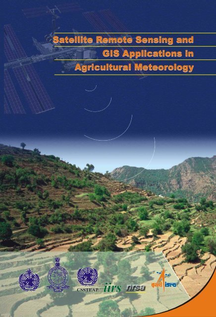
Satellite Remote Sensing and 

GIS Applications in 

Agricultural Meteorology 

Proceedings of the Training Workshop 

7-11 July, 2003, Dehra Dun, India 

Editors 

M.V.K. Sivakumar 

P.S. Roy 

K. Harmsen 

S.K. Saha 

Sponsors 

World Meteorological Organization (WMO) 

India Meteorological Department (IMD) 

Centre for Space Science and Technology Education in Asia and the Pacific 

(CSSTEAP) 

Indian Institute of Remote Sensing (IIRS) 

National Remote Sensing Agency (NRSA) and 

Space Application Centre (SAC) 

AGM-8 

WMO/TD No. 1182 

World Meteorological Organisation 

7bis, Avenue de la Paix 

1211 Geneva 2 

Switzerland 

2004

Published by 


7bis, Avenue de la Paix 

1211 Geneva 2, Switzerland 


All rights reserved. No part of this publication may be reproduced, stored in a retrieval system, 

or transmitted in any form or by any means, electronic, mechanical, photocopying, recording, 

or otherwise, without the prior written consent of the copyright owner. 

Typesetting and Printing : 

M/s Bishen Singh Mahendra Pal Singh 

23-A New Connaught Place, P.O. Box 137, 

Dehra Dun -248001 (Uttaranchal), INDIA 

Ph.: 91-135-2715748 Fax- 91-135-2715107 

E.mail: bsmps@vsnl.com 

Website: http://www.bishensinghbooks.com

FOREWORD

CONTENTS 

Satellite Remote Sensing and GIS Applications in Agricultural .... 1 

Meteorology and WMO Satellite Activities 

– M.V.K. Sivakumar and Donald E. Hinsman 

Principles of Remote Sensing ......... 23 

Shefali Aggarwal 

Earth Resource Satellites ......... 39 

– Shefali Aggarwal 

Meteorological Satellites ......... 67 

– C.M. Kishtawal 

Digital Image Processing ......... 81 

– Minakshi Kumar 

Fundamentals of Geographical Information System ......... 103 

– P.L.N. Raju 

Fundamentals of GPS ......... 121 


Spatial Data Analysis ......... 151 


Retrieval of Agrometeorological Parameters using Satellite ......... 175 

Remote Sensing data 

– S. K. Saha 

Retrieval of Agrometeorological Parameters from Satellites ......... 195 

– C.M. Kishtawal 

Remote Sensing and GIS Application in Agro-ecological ......... 213 

zoning 

– N.R. Patel 

Crop Growth Modeling and its Applications in ......... 235 

Agricultural Meteorology 

– V. Radha Krishna Murthy

Crop Growth and Productivity Monitoring and Simulation ......... 263 

using Remote Sensing and GIS 

– V.K. Dadhwal 

Droughts & Floods Assessment and Monitoring using ......... 291 

Remote Sensing and GIS 

– A.T. Jeyaseelan 

Water and Wind induced Soil Erosion Assessment and ......... 315 

Monitoring using Remote Sensing and GIS 

– S.K. Saha 

Satellite-based Weather Forecasting ......... 331 

– S.R. Kalsi 

Satellite-based Agro-advisory Service ......... 347 

– H. P. Das 

Forest Fire and Degradation Assessment using Satellite Remote ........ 361 

Sensing and Geographic Information System 

– P.S. Roy 

Desert Locust Monitoring System–Remote Sensing and GIS ......... 401 

based approach 

– D. Dutta, S. Bhatawdekar, B. Chandrasekharan, J.R. Sharma, 

S. Adiga, Duncan Wood and Adrian McCardle 

Workshop Evaluation ......... 425 

– M.V.K. Sivakumar

SATELLITE REMOTE SENSING AND GIS 

APPLICATIONS IN AGRICULTURAL METEO- 

ROLOGY AND WMO SATELLITE ACTIVITIES 

M.V.K. Sivakumar and Donald E. Hinsman 

Agricultural Meteorology Division and Satellite Activities Office 

World Meteorological Organization (WMO), 7bis Avenue de la Paix, 

1211 Geneva 2, Switzerland 

Abstract : Agricultural planning and use of agricultural technologies need 

applications of agricultural meteorology. Satellite remote sensing technology is 

increasingly gaining recognition as an important source of agrometeorological data 

as it can complement well the traditional methods agrometeorological data 

collection. Agrometeorologists all over the world are now able to take advantage 

of a wealth of observational data, product and services flowing from specially 

equipped and highly sophisticated environmental observation satellites. In addition, 

Geographic Information Systems (GIS) technology is becoming an essential tool 

for combining various map and satellite information sources in models that simulate 

the interactions of complex natural systems. The Commission for Agricultural 

Meteorology of WMO has been active in the area of remote sensing and GIS 

applications in agrometeorology. The paper provides a brief overview of the satellite 

remote sensing and GIS Applications in agricultural meteorology along with a 

description of the WMO Satellite Activities Programme. The promotion of new 

specialised software should make the applications of the various devices easier, 

bearing in mind the possible combination of several types of inputs such as data 

coming from standard networks, radar and satellites, meteorological and 

climatological models, digital cartography and crop models based on the scientific 

acquisition of the last twenty years. 

INTRODUCTION 

Agricultural planning and use of agricultural technologies need application 

of agricultural meteorology. Agricultural weather and climate data systems are 

necessary to expedite generation of products, analyses and forecasts that affect 

Satellite Remote Sensing and GIS Applications in Agricultural Meteorology 

pp. 1-21

2 Satellite Remote Sensing and GIS Applications in Agricultural Meteorology 

agricultural cropping and management decisions, irrigation scheduling, 

commodity trading and markets, fire weather management and other 

preparedness for calamities, and ecosystem conservation and management. 

Agrometeorological station networks are designed to observe the data of 

meteorological and biological phenomena together with supplementary data 

as disasters and crop damages occur. The method of observation can be 

categorized into two major classes, manually observed and automatic weather 

stations (AWS). A third source for agrometeorological data that is gaining 

recognition for its complementary nature to the traditional methods is satellite 

remote sensing technology. 

Remotely sensed data and AWS systems provide in many ways an 

enhanced and very feasible alternative to manual observation with a very short 

time delay between data collection and transmission. In certain countries where 

only few stations are in operation as in Northern Turkmenistan (Seitnazarov, 

1999), remotely sensed data can improve information on crop conditions for 

an early warning system. Due to the availability of new tools, such as 

Geographic Information Systems (GIS), management of an incredible quantity 

of data such as traditional digital maps, database, models etc., is now possible. 

The advantages are manifold and highly important, especially for the fast crosssector 

interactions and the production of synthetic and lucid information for 

decision-makers. Remote sensing provides the most important informative 

contribution to GIS, which furnishes basic informative layers in optimal time 

and space resolutions. 

In this paper, a brief overview of the satellite remote sensing and GIS 

applications in agricultural meteorology is presented along with a description 

of the WMO Satellite Activities Programme. Details of the various applications 

alluded to briefly in this paper, can be found in the informative papers 

prepared by various experts who will be presenting them in the course of this 

workshop. 

The Commission for Agricultural Meteorology (CAgM) of WMO, Remote 

Sensing and GIS 

Agricultural meteorology had always been an important component of the 

National Meteorological Services since their inception. A formal Commission 

for Agricultural Meteorology (CAgM) which was appointed in 1913 by the 

International Meteorological Organization (IMO), became the foundation of 

the CAgM under WMO in 1951.

M.V.K. Sivakumar and Donald E. Hinsman 3 

The WMO Agricultural Meteorology Programme is coordinated by 

CAgM. The Commission is responsible for matters relating to applications of 

meteorology to agricultural cropping systems, forestry, and agricultural land 

use and livestock management, taking into account meteorological and 

agricultural developments both in the scientific and practical fields and the 

development of agricultural meteorological services of Members by transfer of 

knowledge and methodology and by providing advice. 

CAgM recognized the potential of remote sensing applications in 

agricultural meteorology early in the 70s and at its sixth session in Washington 

in 1974 the Commission agreed that its programme should include studies 

on the application of remote sensing techniques to agrometeorological problems 

and decided to appoint a rapporteur to study the existing state of the 

knowledge of remote sensing techniques and to review its application to 

agrometeorological research and services. At its seventh session in Sofia, Bulgaria 

in 1979, the Commission reviewed the report submitted by Dr A.D. 

Kleschenko (USSR) and Dr J.C. Harlan Jr (USA) and noted that there was a 

promising future for the use in agrometeorology of data from spacecraft and 

aircraft and that rapid progress in this field required exchange of information 

on achievements in methodology and data collection and interpretation. The 

Commission at that time noted that there was a demand in almost all countries 

for a capability to use satellite imagery in practical problems of agrometeorology. 

The Commission continued to pay much attention to both remote sensing 

and GIS applications in agrometeorology in all its subsequent sessions up to 

the 13 th session held in Ljubljana, Slovenia in 2002. Several useful publications 

including Technical Notes and CAgM Reports were published covering the 

use of remote sensing for obtaining agrometeorological information 

(Kleschenko, 1983), operational remote sensing systems in agriculture 

(Kanemasu and Filcroft, 1992), satellite applications to agrometeorology and 

technological developments for the period 1985-89 (Seguin, 1992), statements 

of guidance regarding how well satellite capabilities meet WMO user 

requirements in agrometeorology (WMO, 1998, 2000) etc. At the session in 

Slovenia in 2002, the Commission convened an Expert Team on Techniques 

(including Technologies such as GIS and Remote Sensing) for Agroclimatic 

Characterization and Sustainable Land Management. 

The Commission also recognized that training of technical personnel to 

acquire, process and interpret the satellite imagery was a major task. It was 

felt that acquisition of satellite data was usually much easier than the 

interpretation of data for specific applications that were critical for the


assessment and management of natural resources. In this regard, the 

Commission pointed out that long-term planning and training of technical 

personnel was a key ingredient in ensuring full success in the use of current 

and future remote sensing technologies that could increase and sustain 

agricultural production, especially in the developing countries. In this 

connection, WMO already organized a Training Seminar on GIS and 

Agroecological Zoning in Kuala Lumpur, Malaysia in May 2000 in which six 

participants from Malaysia and 12 from other Asian and the South-West Pacific 

countries participated. The programme for the seminar dealt with 

meteorological and geographical databases, statistical analyses, spatialization, 

agro-ecological classification, overlapping of agroecological zoning with 

boundary layers, data extraction, monitoring system organization and bulletins. 

The training workshop currently being organized in Dehradun is in 

response to the recommendations of the Commission session in Slovenia in 

2002 and it should help the participants from the Asian countries in learning 

new skills and updating their current skills in satellite remote sensing and 

GIS applications in agricultural meteorology. 

GIS APPLICATIONS IN AGROMETEOROLOGY 

A GIS generally refers to a description of the characteristics and tools used 

in the organization and management of geographical data. The term GIS is 

currently applied to computerised storage, processing and retrieval systems 

that have hardware and software specially designed to cope with geographically 

referenced spatial data and corresponding informative attribute. Spatial data 

are commonly in the form of layers that may depict topography or 

environmental elements. Nowadays, GIS technology is becoming an essential 

tool for combining various map and satellite information sources in models 

that simulate the interactions of complex natural systems. A GIS can be used 

to produce images, not just maps, but drawings, animations, and other 

cartographic products. 

The increasing world population, coupled with the growing pressure on 

the land resources, necessitates the application of technologies such as GIS to 

help maintain a sustainable water and food supply according to the 

environmental potential. The “sustainable rural development” concept envisages 

an integrated management of landscape, where the exploitation of natural 

resources, including climate, plays a central role. In this context, 

agrometeorology can help reduce inputs, while in the framework of global


change, it helps quantify the contribution of ecosystems and agriculture to 

carbon budget (Maracchi, 1991). Agroclimatological analysis can improve the 

knowledge of existing problems allowing land planning and optimization of 

resource management. One of the most important agroclimatological 

applications is the climatic risk evaluation corresponding to the possibility that 

certain meteorological events could happen, damaging crops or infrastructure. 

At the national and local level, possible GIS applications are endless. For 

example, agricultural planners might use geographical data to decide on the 

best zones for a cash crop, combining data on soils, topography, and rainfall 

to determine the size and location of biologically suitable areas. The final 

output could include overlays with land ownership, transport, infrastructure, 

labour availability, and distance to market centres. 

The ultimate use of GIS lies in its modelling capability, using real world 

data to represent natural behaviour and to simulate the effect of specific 

processes. Modelling is a powerful tool for analyzing trends and identifying 

factors that affect them, or for displaying the possible consequences of human 

activities that affect the resource availability. 

In agrometeorology, to describe a specific situation, we use all the 

information available on the territory: water availability, soil types, forest and 

grasslands, climatic data, geology, population, land-use, administrative 

boundaries and infrastructure (highways, railroads, electricity or 

communication systems). Within a GIS, each informative layer provides to 

the operator the possibility to consider its influence to the final result. However 

more than the overlap of the different themes, the relationship of the numerous 

layers is reproduced with simple formulas or with complex models. The final 

information is extracted using graphical representation or precise descriptive 

indexes. 

In addition to classical applications of agrometeorology, such as crop yield 

forecasting, uses such as those of the environmental and human security are 

becoming more and more important. For instance, effective forest fire 

prevention needs a series of very detailed information on an enormous scale. 

The analysis of data, such as the vegetation coverage with different levels of 

inflammability, the presence of urban agglomeration, the presence of roads 

and many other aspects, allows the mapping of the areas where risk is greater. 

The use of other informative layers, such as the position of the control points 

and resource availability (staff, cars, helicopters, aeroplanes, fire fighting


equipment, etc.), can help the decision-makers in the management of the 

ecosystems. Monitoring the resources and the meteorological conditions 

therefore allows, the consideration of the dynamics of the system, with more 

adherence to reality. For instance, Figure 1 shows the informative layers used 

for the evaluation of fire risk in Tuscany (Italy). The final map is the result of 

the integration of satellite data with territorial data, through the use of 

implemented GIS technologies (Romanelli et al., 1998). 

Land use Distance road Starting point 

Quota Slope Aspect 

Fire risk 

Figure 1. Informative layers for the evaluation of fire risk index (Maracchi et al., 2000).


These maps of fire risk, constitute a valid tool for foresters and for 

organisation of the public services. At the same time, this new informative 

layer may be used as the base for other evaluations and simulations. Using 

meteorological data and satellite real-time information, it is possible to diversify 

the single situations, advising the competent authorities when the situation 

moves to hazard risks. Modelling the ground wind profile and taking into 

account the meteorological conditions, it is possible to advise the operators 

of the change in the conditions that can directly influence the fire, allowing 

the modification of the intervention strategies. 

An example of preliminary information system to country scale is given 

by the SISP (Integrated information system for monitoring cropping season 

by meteorological and satellite data), developed to allow the monitoring of 

the cropping season and to provide an early warning system with useful 

information about evolution of crop conditions (Di Chiara and Maracchi, 

1994). The SISP uses: 

• Statistical analysis procedures on historical series of rainfall data to produce 

agroclimatic classification; 

• A crop (millet) simulation model to estimate millet sowing date and to 

evaluate the effect of the rainfall distribution on crop growth and yield; 

• NOAA-NDVI image analysis procedures in order to monitor vegetation 

condition; 

• Analysis procedures of Meteosat images of estimated rainfall for early 

prediction of sowing date and risk areas. 

The results of SISP application shown for Niger (Fig. 2) are charts and 

maps, which give indications to the expert of the millet conditions during 

the season in Niger, with the possibility to estimate the moment of the harvest 

and final production. SISP is based on the simulation of the millet growth 

and it gives an index of annual productivity by administrative units. These 

values, multiplied to a yield statistical factor, allow estimation of absolute 

production. 

By means of such systems based on modelling and remote sensing, it is 

possible to extract indices relative to the main characteristics of the agricultural 

season and conditions of natural systems. This system is less expensive, easily 

transferable and requires minor informative layers, adapting it to the specific 

requirements of the users.


Niamey, cropping season 1993 

Characterization of land productivity at Niger 

CeSIA Index for miller 

Elaborated on 10 years (1981-90) and 120 stations 

Rainfall Cultural Coeff. Water balance 

Longitude 

Figure 2. Examples of outputs of SISP (Maracchi et al., 2000). 

SATELLITE REMOTE SENSING 

Remote sensing provides spatial coverage by measurement of reflected and 

emitted electromagnetic radiation, across a wide range of wavebands, from the 

earth’s surface and surrounding atmosphere. The improvement in technical 

tools of meteorological observation, during the last twenty years, has created 

a favourable substratum for research and monitoring in many applications of 

sciences of great economic relevance, such as agriculture and forestry. Each 

waveband provides different information about the atmosphere and land 

surface: surface temperature, clouds, solar radiation, processes of photosynthesis 

and evaporation, which can affect the reflected and emitted radiation, detected 

by satellites. The challenge for research therefore is to develop new systems 

extracting this information from remotely sensed data, giving to the final users, 

near-real-time information. 

Over the last two decades, the development of space technology has led 

to a substantial increase in satellite earth observation systems. Simultaneously, 

the Information and Communication Technology (ICT) revolution has rendered 

increasingly effective the processing of data for specific uses and their 

instantaneous distribution on the World Wide Web (WWW). 

The meteorological community and associated environmental disciplines 

such as climatology including global change, hydrology and oceanography all 

over the world are now able to take advantage of a wealth of observational 

data, products and services flowing from specially equipped and highly 

sophisticated environmental observation satellites. An environmental


observation satellite is an artificial Earth satellite providing data on the Earth 

system and a Meteorological satellite is a type of environmental satellite 

providing meteorological observations. Several factors make environmental 

satellite data unique compared with data from other sources, and it is worthy 

to note a few of the most important: 

• Because of its high vantage point and broad field of view, an environmental 

satellite can provide a regular supply of data from those areas of the globe 

yielding very few conventional observations; 

• The atmosphere is broadly scanned from satellite altitude and enables largescale 

environmental features to be seen in a single view; 

• The ability of certain satellites to view a major portion of the atmosphere 

continually from space makes them particularly well suited for the 

monitoring and warning of short-lived meteorological phenomena; and 

• The advanced communication systems developed as an integral part of 

the satellite technology permit the rapid transmission of data from the 

satellite, or their relay from automatic stations on earth and in the 

atmosphere, to operational users. 

These factors are incorporated in the design of meteorological satellites to 

provide data, products and services through three major functions: 

• Remote sensing of spectral radiation which can be converted into 

meteorological measurements such as cloud cover, cloud motion vectors, 

surface temperature, vertical profiles of atmospheric temperature, humidity 

and atmospheric constituents such as ozone, snow and ice cover, ozone 

and various radiation measurements; 

• Collection of data from in situ sensors on remote fixed or mobile platforms 

located on the earth’s surface or in the atmosphere; and 

• Direct broadcast to provide cloud-cover images and other meteorological 

information to users through a user-operated direct readout station. 

The first views of earth from space were not obtained from satellites but 

from converted military rockets in the early 1950s. It was not until 1 April 

1960 that the first operational meteorological satellite, TIROS-I, was launched


by the USA and began to transmit basic, but very useful, cloud imagery. This 

satellite was such an effective proof of concept that by 1966 the USA had 

launched a long line of operational polar satellites and its first geostationary 

meteorological satellite. In 1969 the USSR launched the first of a series of 

polar satellites. In 1977 geostationary meteorological satellites were also 

launched and operated by Japan and by the European Space Agency (ESA). 

Thus, within 18 years of the first practical demonstration by TIROS-I, a fully 

operational meteorological satellite system (Fig. 3) was in place, giving routine 

data coverage of most of the planet. This rapid evolution of a very expensive 

new system was unprecedented and indicates the enormous value of these 

satellites to meteorology and society. Some four decades after the first earth 

images, new systems are still being designed and implemented, illustrating 

the continued and dynamic interest in this unique source of environmental 

data. 

Figure 3: Nominal configuration of the space-based sub-system of the Global Observing 

System in 1978.


By the year 2000, WMO Members contributing to the space-based subsystem 

of the Global Observing System had grown. There were two major 

constellations in the space-based Global Observing System (GOS) (Fig. 4). 

One constellation was the various geostationary satellites, which operated in 

an equatorial belt and provided a continuous view of the weather from roughly 

70°N to 70°S. The second constellation in the current space-based GOS 

comprised the polar-orbiting satellites operated by the Russian Federation, 

the USA and the People’s Republic of China. The METEOR-3 series has been 

operated by the Russian Federation since 1991. 

Figure 4: Nominal configuration of the space-based sub-system of the Global Observing 

System in 2000. 

The ability of geostationary satellites to provide a continuous view of 

weather systems make them invaluable in following the motion, development, 

and decay of such phenomena. Even such short-term events such as severe 

thunderstorms, with a life-time of only a few hours, can be successfully 

recognized in their early stages and appropriate warnings of the time and area


of their maximum impact can be expeditiously provided to the general public. 

For this reason, its warning capability has been the primary justification for 

the geostationary spacecraft. Since 71 per cent of the Earth’s surface is water 

and even the land areas have many regions which are sparsely inhabited, the 

polar-orbiting satellite system provides the data needed to compensate the 

deficiencies in conventional observing networks. Flying in a near-polar orbit, 

the spacecraft is able to acquire data from all parts of the globe in the course 

of a series of successive revolutions. For these reasons the polar-orbiting satellites 

are principally used to obtain: (a) daily global cloud cover; and (b) accurate 

quantitative measurements of surface temperature and of the vertical variation 

of temperature and water vapour in the atmosphere. There is a distinct 

advantage in receiving global data acquired by a single set of observing sensors. 

Together, the polar-orbiting and geostationary satellites constitute a truly global 

meteorological satellite network. 

Satellite data provide better coverage in time and in area extent than any 

alternative. Most polar satellite instruments observe the entire planet once or 

twice in a 24-hour period. Each geostationary satellite’s instruments cover 

about ¼ of the planet almost continuously and there are now six geostationary 

satellites providing a combined coverage of almost 75%. Satellites cover the 

world’s oceans (about 70% of the planet), its deserts, forests, polar regions, 

and other sparsely inhabited places. Surface winds over the oceans from satellites 

are comparable to ship observations; ocean heights can be determined to a 

few centimetres; and temperatures in any part of the atmosphere anywhere 

in the world are suitable for computer models. It is important to make 

maximum use of this information to monitor our environment. Access to these 

satellite data and products is only the beginning. In addition, the ability to 

interpret, combine, and make maximum use of this information must be an 

integral element of national management in developed and developing 

countries. 

The thrust of the current generation of environmental satellites is aimed 

primarily at characterizing the kinematics and dynamics of the atmospheric 

circulation. The existing network of environmental satellites, forming part of 

the GOS of the World Weather Watch produces real-time weather information 

on a regular basis. This is acquired several times a day through direct broadcast 

from the meteorological satellites by more than 1,300 stations located in 125 

countries.


The ground segment of the space-based component of the GOS should 

provide for the reception of signals and DCP data from operational satellites 

and/or the processing, formatting and display of meaningful environmental 

observation information, with a view to further distributing it in a convenient 

form to local users, or over the GTS, as required. This capability is normally 

accomplished through receiving and processing stations of varying complexity, 

sophistication and cost. 

In addition to their current satellite programmes in polar and geostationary 

orbits, satellite operators in the USA (NOAA) and Europe (EUMETSAT) have 

agreed to launch a series of joint polar-orbiting satellites (METOP) in 2005. 

These satellites will complement the existing global array of geostationary 

satellites that form part of the Global Observing System of the World 

Meteorological Organization. This Initial Joint Polar System (IJPS) represents 

a major cooperation programme between the USA and Europe in the field of 

space activities. Europe has invested 2 billion Euros in a low earth orbit satellite 

system, which will be available operationally from 2006 to 2020. 

The data provided by these satellites will enable development of 

operational services in improved temperature and moisture sounding for 

numerical weather prediction (NWP), tropospheric/stratospheric interactions, 

imagery of clouds and land/ocean surfaces, air-sea interactions, ozone and other 

trace gases mapping and monitoring, and direct broadcast support to 

nowcasting. Advanced weather prediction models are needed to assimilate 

satellite information at the highest possible spatial and spectral resolutions. 

It imposes new requirements on the precision and spectral resolution of 

soundings in order to improve the quality of weather forecasts. Satellite 

information is already used by fishery-fleets on an operational basis. Wind 

and the resulting surface stress is the major force for oceanic motions. Ocean 

circulation forecasts require the knowledge of an accurate wind field. Wind 

measurements from space play an increasing role in monitoring of climate 

change and variability. The chemical composition of the troposphere is 

changing on all spatial scales. Increases in trace gases with long atmospheric 

residence times can affect the climate and chemical equilibrium of the Earth/ 

Atmosphere system. Among these trace gases are methane, nitrogen dioxide, 

and ozone. The chemical and dynamic state of the stratosphere influence the 

troposphere by exchange processes through the tropopause. Continuous 

monitoring of ozone and of (the main) trace gases in the troposphere and the 

stratosphere is an essential input to the understanding of the related 

atmospheric chemistry processes.


WMO SPACE PROGRAMME 

The World Meteorological Organization, a specialized agency of the United 

Nations, has a membership of 187 states and territories (as of June 2003). 

Amongst the many programmes and activities of the organization, there are 

three areas which are particularly pertinent to the satellite activities: 

• To facilitate world-wide cooperation in the establishment of networks for 

making meteorological, as well as hydrological and other geophysical 

observations and centres to provide meteorological services; 

• To promote the establishment and maintenance of systems for the rapid 

exchange of meteorological and related information; 

• To promote the standardization of meteorological observations and ensure 

the uniform publication of observations and statistics. 

The Fourteenth WMO Congress, held in May 2003, initiated a new Major 

Programme, the WMO Space Programme, as a cross-cutting programme to 

increase the effectiveness and contributions from satellite systems to WMO 

Programmes. Congress recognized the critical importance for data, products 

and services provided by the World Weather Watch’s (WWW) expanded spacebased 

component of the Global Observing System (GOS) to WMO 

Programmes and supported Programmes. During the past four years, the use 

by WMO Members of satellite data, products and services has experienced 

tremendous growth to the benefit of almost all WMO Programmes and 

supported Programmes. The decision by the fifty-third Executive Council to 

expand the space-based component of the Global Observing System to include 

appropriate R&D environmental satellite missions was a landmark decision 

in the history of WWW. Congress agreed that the Commission for Basic 

Systems (CBS) should continue the lead role in full consultation with the other 

technical commissions for the new WMO Space Programme. Congress also 

decided to establish WMO Consultative Meetings on High-level Policy on 

Satellite Matters. The Consultative Meetings will provide advice and guidance 

on policy-related matters and maintain a high level overview of the WMO 

Space Programme. The expected benefits from the new WMO Space 

Programme include an increasing contribution to the development of the 

WWW’s GOS, as well as to the other WMO-supported programmes and 

associated observing systems through the provision of continuously improved 

data, products and services, from both operational and R&D satellites, and


to facilitate and promote their wider availability and meaningful utilization 

around the globe. 

The main thrust of the WMO Space Programme Long-term Strategy is: 

“To make an increasing contribution to the development of the WWW’s 

GOS, as well as to the other WMO-supported Programmes and associated 

observing systems (such as AREP’s GAW, GCOS, WCRP, HWR’s WHYCOS 

and JCOMM’s implementation of GOS) through the provision of continuously 

improved data, products and services, from both operational and R&D 

satellites, and to facilitate and promote their wider availability and meaningful 

utilization around the globe”. 

The main elements of the WMO Space Programme Long-term Strategy 

are as follows: 

(a) Increased involvement of space agencies contributing, or with the 

potential to contribute to, the space-based component of the GOS; 

(b) Promotion of a wider awareness of the availability and utilization of 

data, products - and their importance at levels 1, 2, 3 or 4 - and 

services, including those from R&D satellites; 

(c) Considerably more attention to be paid to the crucial problems 

connected with the assimilation of R&D and new operational data 

streams in nowcasting, numerical weather prediction systems, 

reanalysis projects, monitoring climate change, chemical composition 

of the atmosphere, as well as the dominance of satellite data in some 

cases; 

(d) Closer and more effective cooperation with relevant international 

bodies; 

(e) Additional and continuing emphasis on education and training; 

(f ) Facilitation of the transition from research to operational systems; 

(g) Improved integration of the space component of the various observing 

systems throughout WMO Programmes and WMO-supported 

Programmes;


(h) Increased cooperation amongst WMO Members to develop common 

basic tools for utilization of research, development and operational 

remote sensing systems. 

Coordination Group for Meteorological Satellites (CGMS) 

In 1972 a group of satellite operators formed the Co-ordination of 

Geostationary Meteorological Satellites (CGMS) that would be expanded in 

the early 1990s to include polar-orbiting satellites and changed its name - 

but not its abbreviation - to the Co-ordination Group for Meteorological 

Satellites. The Co-ordination Group for Meteorological Satellites (CGMS) 

provides a forum for the exchange of technical information on geostationary 

and polar orbiting meteorological satellite systems, such as reporting on current 

meteorological satellite status and future plans, telecommunication matters, 

operations, inter-calibration of sensors, processing algorithms, products and 

their validation, data transmission formats and future data transmission 

standards. 

Since 1972, the CGMS has provided a forum in which the satellite 

operators have studied jointly with the WMO technical operational aspects 

of the global network, so as to ensure maximum efficiency and usefulness 

through proper coordination in the design of the satellites and in the 

procedures for data acquisition and dissemination. 

Membership of CGMS 

The table of members shows the lead agency in each case. Delegates are often 

supported by other agencies, for example, ESA (with EUMETSAT), NASDA 

(with Japan) and NASA (with NOAA). 

The current Membership of CGMS is: 

EUMETSAT joined 1987 

currently CGMS Secretariat 

India Meteorological Department joined 1979 

Japan Meteorological Agency founder member, 1972 

China Meteorological Administration joined 1989 

NOAA/NESDIS founder member, 1972 

Hydromet Service of the Russian Federation joined 1973


WMO joined 1973 

IOC of UNESCO joined 2000 

NASA joined 2002 

ESA joined 2002 

NASDA joined 2002 

Rosaviakosmos joined 2002 

WMO, in its endeavours to promote the development of a global 

meteorological observing system, participated in the activities of CGMS from 

its first meeting. There are several areas where joint consultations between the 

satellite operators and WMO are needed. The provision of data to 

meteorological centres in different parts of the globe is achieved by means of 

the Global Telecommunication System (GTS) in near-real-time. This 

automatically involves assistance by WMO in developing appropriate code 

forms and provision of a certain amount of administrative communications 

between the satellite operators. 

WMO’s role within CGMS would be to state the observational and system 

requirements for WMO and supported programmes as they relate to the 

expanded space-based components of the GOS, GAW, GCOS and WHYCOS. 

CGMS satellite operators would make their voluntary commitments to meet 

the stated observational and system requirements. WMO would, through its 

Members, strive to provide CGMS satellite operators with operational and preoperational 

evaluations of the benefit and impacts of their satellite systems. 

WMO would also act as a catalyst to foster direct user interactions with the 

CGMS satellite operators through available means such as conferences, 

symposia and workshops. 

The active involvement of WMO has allowed the development and 

implementation of the operational ASDAR system as a continuing part of the 

Global Observing System. Furthermore, the implementation of the IDCS 

system was promoted by WMO and acted jointly with the satellite operators 

as the admitting authority in the registration procedure for IDCPs. 

The expanded space-based component of the world weather watch’s global 

observing system 

Several initiatives since 2000 with regard to WMO satellite activities have 

culminated in an expansion of the space-based component of the Global


Observing System to include appropriate Research and Development (R&D) 

satellite missions. The recently established WMO Consultative Meetings on 

High-Level Policy on Satellite Matters have acted as a catalyst in each of these 

interwoven and important areas. First was the establishment of a new series 

of technical documents on the operational use of R&D satellite data. Second 

was a recognition of the importance of R&D satellite data in meeting WMO 

observational data requirements and the subsequent development of a set of 

Guidelines for requirements for observational data from operational and R&D 

satellite missions. Third have been the responses by the R&D space agencies 

in making commitments in support of the system design for the space-based 

component of the Global Observing System. And lastly has been WMO’s 

recognition that it should have a more appropriate programme structure - a 

WMO Space Programme - to capitalize on the full potential of satellite data, 

products and services from both the operational and R&D satellites. 

WMO Members’ responses to the request for input for the report on the 

utility of R&D satellite data and products covered the full spectrum of WMO 

Regions as well as a good cross-section of developed and developing countries. 

Countries from both the Northern and Southern Hemispheres, tropical, midand 

high-latitude as well as those with coastlines and those landlocked had 

responded. Most disciplines and application areas including NWP, hydrology, 

climate, oceanography, agrometeorology, environmental monitoring and 

detection and monitoring of natural disasters were included. 

A number of WMO Programmes and associated application areas 

supported by data and products from the R&D satellites. While not complete, 

the list included specific applications within the disciplines of agrometeorology, 

weather forecasting, hydrology, climate and oceanography including: 

monitoring of ecology, sea-ice, snow cover, urban heat island, crop yield, 

vegetation, flood, volcanic ash and other natural disasters; tropical cyclone 

forecasting; fire areas; oceanic chlorophyll content; NWP; sea height; and CO 2 

exchange between the atmosphere and ocean. 

WMO agreed that there was an increasing convergence between research 

and operational requirements for the space-based component of the Global 

Observing System and that WMO should seek to establish a continuum of 

requirements for observational data from R&D satellite missions to operational 

missions. WMO endorsed the Guidelines for requirements for observational data 

from operational and R&D satellite missions to provide operational users a 

measure of confidence in the availability of operational and R&D observational 

data, and data providers with an indication of its utility.


The inclusion of R&D satellite systems into the space-based component 

of GOS would more than double the need for external coordination 

mechanisms. Firstly, there will be unique coordination needs between WMO 

and R&D space agencies. Secondly, there will be coordination needs between 

operational and R&D space agencies in such areas as frequency coordination, 

orbit coordination including equator crossing-times, standardization of data 

formats, standardization of user stations. Figure 5 shows the present spacebased 

sub-system of the Global Observing System with the new R&D 

constellation including NASA’s Aqua, Terra, NPP, TRMM, QuikSCAT and 

GPM missions, ESA’s ENVISAT, ERS-1 and ERS-2 missions, NASDA’s 

ADEOS II and GCOM series, Rosaviakosmos’s research instruments on board 

ROSHYDROMET’s operational METEOR 3M Nl satellite, as well as on its 

future Ocean series and CNES’s JASON-1 and SPOT-5. 

Figure 5: Space-based sub-system of the Global Observing System in 2003. 

To better satisfy the needs of all WMO and supported programmes for 

satellite data, products and services from both operational and R&D satellites 

and in consideration of the increasing role of both types of satellites, WMO 

felt it appropriate to propose an expansion of the present mechanisms for


coordination within the WMO structure and cooperation between WMO and 

the operators of operational meteorological satellites and R&D satellites. In 

doing so, WMO felt that an effective means to improve cooperation with both 

operational meteorological and R&D satellite operators would be through an 

expanded CGMS that would include those R&D space agencies contributing 

to the space-based component of the GOS. 

WMO agreed that the WMO satellite activities had grown and that it 

was now appropriate to establish a WMO Space Programme as a matter of 

priority. The scope, goals and objectives of the new programme should respond 

to the tremendous growth in the utilization of environmental satellite data, 

products and services within the expanded space-based component of the GOS 

that now include appropriate Research and Development environmental 

satellite missions. The Consultative Meetings on High-Level Policy on Satellite 

Matters should be institutionalized in order to more formally establish the 

dialogue and participation of environmental satellite agencies in WMO matters. 

In considering the important contributions made by environmental satellite 

systems to WMO and its supported programmes as well as the large 

expenditures by the space agencies, WMO felt it appropriate that the overall 

responsibility for the new WMO Space Programme should be assigned to CBS 

and a new institutionalized Consultative Meetings on High-Level Policy on 

Satellite Matters. 

CONCLUSIONS 

Recent developments in remote sensing and GIS hold much promise to 

enhance integrated management of all available information and the extraction 

of desired information to promote sustainable agriculture and development. 

Active promotion of the use of remote sensing and GIS in the National 

Meteorological and Hydrological Services (NMHSs), could enhance improved 

agrometeorological applications. To this end it is important to reinforce training 

in these new fields. The promotion of new specialised software should make 

the applications of the various devices easier, bearing in mind the possible 

combination of several types of inputs such as data coming from standard 

networks, radar and satellites, meteorological and climatological models, digital 

cartography and crop models based on the scientific acquisition of the last 

twenty years. International cooperation is crucial to promote the much needed 

applications in the developing countries and the WMO Space Programme 

actively promotes such cooperation throughout all WMO Programmes and 

provides guidance to these and other multi-sponsored programmes on the 

potential of remote sensing techniques in meteorology, hydrology and related


disciplines, as well as in their applications. The new WMO Space Programme 

will further enhance both external and internal coordination necessary to 

maximize the exploitation of the space-based component of the GOS to provide 

valuable satellite data, products and services to WMO Members towards 

meeting observational data requirements for WMO programmes more so than 

ever before in the history of the World Weather Watch. 

REFERENCES 

Di Chiara, C. and G. Maracchi. 1994. Guide au S.I.S.P. ver. 1.0. Technical Manual No. 14, 

CeSIA, Firenze, Italy. 

Kleschenko, A.D. 1983. Use of remote sensing for obtaining agrometeorological information. 

CAgM Report No. 12, Part I. Geneva, Switzerland: World Meteorological Organization. 

Kanemasu, E.T. and I.D. Filcroft. 1992. Operational remote sensing systems in agriculture. 

CAgM Report No. 50, Part I. Geneva, Switzerland: World Meteorological Organization. 

Maracchi, G. 1991. Agrometeorologia : stato attuale e prospettive future. Proc. Congress 

Agrometeorologia e Telerilevamento. Agronica, Palermo, Italy, pp. 1-5. 

Maracchi, G., V. Pérarnaud and A.D. Kleschenko. 2000. Applications of geographical 

information systems and remote sensing in agrometeorology. Agric. For. Meteorol. 

103:119-136. 

Romanelli, S., L. Bottai and F. Maselli. 1998. Studio preliminare per la stima del rischio 

d’incendio boschivo a scala regionale per mezzo dei dati satellitari e ausilari. Tuscany 

Region - Laboratory for Meteorology and Environmental Modelling (LaMMA), Firenze, 

Italy. 

Seguin, B. 1992. Satellite applications to agrometeorology: technological developments for 

the period 1985-1989. CAgM Report No. 50, Part II. Geneva, Switzerland: World 

Meteorological Organization. 

Seitnazarov, 1999. Technology and methods of collection, distribution and analyzing of 

agrometeorological data in Dashhovuz velajat, Turkmenistan. In: Contributions from 

members on Operational Applications in the International Workshop on 

Agrometeorology in the 21 st Century: Needs and Perspectives, Accra, Ghana. CAgM 

Report No. 77, Geneva, Switzerland: World Meteorological Organization. 

WMO. 1998. Preliminary statement of guidance regarding how well satellite capabilities 

meet WMO user requirements in several application areas, SAT-21, WMO/TD No. 

913, Geneva, Switzerland: World Meteorological Organization. 

WMO. 2000. Statement of guidance regarding how well satellite capabilities meet wmo 

user requirements in several application areas. SAT-22, WMO/TD No. 992, Geneva, 

Switzerland: World Meteorological Organization.

PRINCIPLES OF REMOTE SENSING 


Photogrammetry and Remote Sensing Division 

Indian Institute of Remote Sensing, Dehra Dun 

Abstract : Remote sensing is a technique to observe the earth surface or the 

atmosphere from out of space using satellites (space borne) or from the air using 

aircrafts (airborne). Remote sensing uses a part or several parts of the 

electromagnetic spectrum. It records the electromagnetic energy reflected or emitted 

by the earth’s surface. The amount of radiation from an object (called radiance) is 

influenced by both the properties of the object and the radiation hitting the object 

(irradiance). The human eyes register the solar light reflected by these objects and 

our brains interpret the colours, the grey tones and intensity variations. In remote 

sensing various kinds of tools and devices are used to make electromagnetic radiation 

outside this range from 400 to 700 nm visible to the human eye, especially the 

near infrared, middle-infrared, thermal-infrared and microwaves. 

Remote sensing imagery has many applications in mapping land-use and cover, 

agriculture, soils mapping, forestry, city planning, archaeological investigations, 

military observation, and geomorphological surveying, land cover changes, 

deforestation, vegetation dynamics, water quality dynamics, urban growth, etc. This 

paper starts with a brief historic overview of remote sensing and then explains the 

various stages and the basic principles of remotely sensed data collection mechanism. 

INTRODUCTION 

Remote sensing (RS), also called earth observation, refers to obtaining 

information about objects or areas at the Earth’s surface without being 

in direct contact with the object or area. Humans accomplish this task with 

aid of eyes or by the sense of smell or hearing; so, remote sensing is day-today 

business for people. Reading the newspaper, watching cars driving in front 

of you are all remote sensing activities. Most sensing devices record information 

about an object by measuring an object’s transmission of electromagnetic energy 

from reflecting and radiating surfaces. 


pp. 23-38

24 Principles of Remote Sensing 

Remote sensing techniques allow taking images of the earth surface in 

various wavelength region of the electromagnetic spectrum (EMS). One of the 

major characteristics of a remotely sensed image is the wavelength region it 

represents in the EMS. Some of the images represent reflected solar radiation 

in the visible and the near infrared regions of the electromagnetic spectrum, 

others are the measurements of the energy emitted by the earth surface itself 

i.e. in the thermal infrared wavelength region. The energy measured in the 

microwave region is the measure of relative return from the earth’s surface, 

where the energy is transmitted from the vehicle itself. This is known as active 

remote sensing, since the energy source is provided by the remote sensing 

platform. Whereas the systems where the remote sensing measurements 

depend upon the external energy source, such as sun are referred to as passive 

remote sensing systems. 

PRINCIPLES OF REMOTE SENSING 

Detection and discrimination of objects or surface features means detecting 

and recording of radiant energy reflected or emitted by objects or surface 

material (Fig. 1). Different objects return different amount of energy in different 

bands of the electromagnetic spectrum, incident upon it. This depends on 

the property of material (structural, chemical, and physical), surface roughness, 

angle of incidence, intensity, and wavelength of radiant energy. 

The Remote Sensing is basically a multi-disciplinary science which includes 

a combination of various disciplines such as optics, spectroscopy, photography, 

computer, electronics and telecommunication, satellite launching etc. All these 

technologies are integrated to act as one complete system in itself, known as 

Remote Sensing System. There are a number of stages in a Remote Sensing 

process, and each of them is important for successful operation. 

Stages in Remote Sensing 

• Emission of electromagnetic radiation, or EMR (sun/self- emission) 

• Transmission of energy from the source to the surface of the earth, as well 

as absorption and scattering 

• Interaction of EMR with the earth’s surface: reflection and emission 

• Transmission of energy from the surface to the remote sensor 

• Sensor data output

Shefali Aggarwal 25 

Satellite 

Sun 

Reflected 

Solar Radiation 

Pre-Process and Archive 

Down Link 

Atmosphere 

Distribute for Analysis 

Forest 

Water 

Grass 

Bare Soil 

Paved 

Road 

Built-up Area 

• Data transmission, processing and analysis 

What we see 

Figure 1: Remote Sensing process 

At temperature above absolute zero, all objects radiate electromagnetic 

energy by virtue of their atomic and molecular oscillations. The total amount 

of emitted radiation increases with the body’s absolute temperature and peaks 

at progressively shorter wavelengths. The sun, being a major source of energy, 

radiation and illumination, allows capturing reflected light with conventional 

(and some not-so-conventional) cameras and films. 

The basic strategy for sensing electromagnetic radiation is clear. Everything 

in nature has its own unique distribution of reflected, emitted and absorbed 

radiation. These spectral characteristics, if ingeniously exploited, can be used 

to distinguish one thing from another or to obtain information about shape, 

size and other physical and chemical properties. 

Modern Remote Sensing Technology versus Conventional Aerial Photography 

The use of different and extended portions of the electromagnetic 

spectrum, development in sensor technology, different platforms for remote 

sensing (spacecraft, in addition to aircraft), emphasize on the use of spectral 

information as compared to spatial information, advancement in image 

processing and enhancement techniques, and automated image analysis in 

addition to manual interpretation are points for comparison of conventional 

aerial photography with modern remote sensing system.


During early half of twentieth century, aerial photos were used in military 

surveys and topographical mapping. Main advantage of aerial photos has been 

the high spatial resolution with fine details and therefore they are still used 

for mapping at large scale such as in route surveys, town planning, 

construction project surveying, cadastral mapping etc. Modern remote sensing 

system provide satellite images suitable for medium scale mapping used in 

natural resources surveys and monitoring such as forestry, geology, watershed 

management etc. However the future generation satellites are going to provide 

much high-resolution images for more versatile applications. 

HISTORIC OVERVIEW 

In 1859 Gaspard Tournachon took an oblique photograph of a small village 

near Paris from a balloon. With this picture the era of earth observation and 

remote sensing had started. His example was soon followed by other people 

all over the world. During the Civil War in the United States aerial 

photography from balloons played an important role to reveal the defence 

positions in Virginia (Colwell, 1983). Likewise other scientific and technical 

developments this Civil War time in the United States speeded up the 

development of photography, lenses and applied airborne use of this 

technology. Table 1 shows a few important dates in the development of remote 

sensing. 

The next period of fast development took place in Europe and not in the 

United States. It was during World War I that aero planes were used on a 

large scale for photoreconnaissance. Aircraft proved to be more reliable and 

more stable platforms for earth observation than balloons. In the period 

between World War I and World War II a start was made with the civilian 

use of aerial photos. Application fields of airborne photos included at that 

time geology, forestry, agriculture and cartography. These developments lead 

to much improved cameras, films and interpretation equipment. The most 

important developments of aerial photography and photo interpretation took 

place during World War II. During this time span the development of other 

imaging systems such as near-infrared photography; thermal sensing and radar 

took place. Near-infrared photography and thermal-infrared proved very 

valuable to separate real vegetation from camouflage. The first successful 

airborne imaging radar was not used for civilian purposes but proved valuable 

for nighttime bombing. As such the system was called by the military ‘plan 

position indicator’ and was developed in Great Britain in 1941.


After the wars in the 1950s remote sensing systems continued to evolve 

from the systems developed for the war effort. Colour infrared (CIR) 

photography was found to be of great use for the plant sciences. In 1956 

Colwell conducted experiments on the use of CIR for the classification and 

recognition of vegetation types and the detection of diseased and damaged or 

stressed vegetation. It was also in the 1950s that significant progress in radar 

technology was achieved. 

Table1: Milestones in the History of Remote Sensing 

1800 Discovery of Infrared by Sir W. Herschel 

1839 Beginning of Practice of Photography 

1847 Infrared Spectrum Shown by J.B.L. Foucault 

1859 Photography from Balloons 

1873 Theory of Electromagnetic Spectrum by J.C. Maxwell 

1909 Photography from Airplanes 

1916 World War I: Aerial Reconnaissance 

1935 Development of Radar in Germany 

1940 WW II: Applications of Non-Visible Part of EMS 

1950 Military Research and Development 

1959 First Space Photograph of the Earth (Explorer-6) 

1960 First TIROS Meteorological Satellite Launched 

1970 Skylab Remote Sensing Observations from Space 

1972 Launch Landsat-1 (ERTS-1) : MSS Sensor 

1972 Rapid Advances in Digital Image Processing 

1982 Launch of Landsat -4 : New Generation of Landsat Sensors: TM 

1986 French Commercial Earth Observation Satellite SPOT 

1986 Development Hyperspectral Sensors 

1990 Development High Resolution Space borne Systems 

First Commercial Developments in Remote Sensing 

1998 Towards Cheap One-Goal Satellite Missions 

1999 Launch EOS : NASA Earth Observing Mission 

1999 Launch of IKONOS, very high spatial resolution sensor system


ELECTROMAGNETIC RADIATION AND THE ELECTROMAGNETIC 

SPECTRUM 

EMR is a dynamic form of energy that propagates as wave motion at a velocity 

of c = 3 x 10 10 cm/sec. The parameters that characterize a wave motion are 

wavelength (λ), frequency (ν) and velocity (c) (Fig. 2). The relationship 

between the above is 

c = νλ. 

Figure 2: Electromagnetic wave. It has two components, Electric field E and Magnetic 

field M, both perpendicular to the direction of propagation 

Electromagnetic energy radiates in accordance with the basic wave theory. 

This theory describes the EM energy as travelling in a harmonic sinusoidal 

fashion at the velocity of light. Although many characteristics of EM energy 

are easily described by wave theory, another theory known as particle theory 

offers insight into how electromagnetic energy interacts with matter. It suggests 

that EMR is composed of many discrete units called photons/quanta. The 

energy of photon is 

Where 

Q is the energy of quantum, 

h = Planck’s constant 

Q = hc / λ = h ν


Table 2: Principal Divisions of the Electromagnetic Spectrum 

Wavelength 

Gamma rays 

X-rays 

Ultraviolet (UV) region 

0.30 µm - 0.38 µm 

(1µm = 10 -6 m) 

Visible Spectrum 

0.4 µm - 0.7 µm 

Violet 0.4 µm -0.446 µm 

Blue 0.446 µm -0.5 µm 

Green 0.5 µm - 0.578 µm 

Yellow 0.578 µm - 0.592 µm 

Orange 0.592 µm - 0.62 µm 

Red 0.62 µm -0.7 µm 

Infrared (IR) Spectrum 

0.7 µm – 100 µm 

Microwave Region 

1 mm - 1 m 

Radio Waves 

(>1 m) 

Description 

Gamma rays 

X-rays 

This region is beyond the violet portion of the visible 

wavelength, and hence its name. Some earth’s surface 

material primarily rocks and minerals emit visible UV 

radiation. However UV radiation is largely scattered 

by earth’s atmosphere and hence not used in field of 

remote sensing. 

This is the light, which our eyes can detect. This is 

the only portion of the spectrum that can be 

associated with the concept of color. Blue Green and 

Red are the three primary colors of the visible 

spectrum. They are defined as such because no single 

primary color can be created from the other two, but 

all other colors can be formed by combining the 

three in various proportions. The color of an object 

is defined by the color of the light it reflects. 

Wavelengths longer than the red portion of the 

visible spectrum are designated as the infrared 

spectrum. British Astronomer William Herschel 

discovered this in 1800. The infrared region can be 

divided into two categories based on their radiation 

properties. 

Reflected IR (.7 µm - 3.0 µm) is used for remote 

sensing. Thermal IR (3 µm - 35 µm) is the radiation 

emitted from earth’s surface in the form of heat and 

used for remote sensing. 

This is the longest wavelength used in remote sensing. 

The shortest wavelengths in this range have 

properties similar to thermal infrared region. The 

main advantage of this spectrum is its ability to 

penetrate through clouds. 

This is the longest portion of the spectrum mostly 

used for commercial broadcast and meteorology.


Types of Remote Sensing 

Remote sensing can be either passive or active. ACTIVE systems have their 

own source of energy (such as RADAR) whereas the PASSIVE systems depend 

upon external source of illumination (such as SUN) or self-emission for remote 

sensing. 

INTERACTION OF EMR WITH THE EARTH’S SURFACE 

Radiation from the sun, when incident upon the earth’s surface, is either 

reflected by the surface, transmitted into the surface or absorbed and emitted 

by the surface (Fig. 3). The EMR, on interaction, experiences a number of 

changes in magnitude, direction, wavelength, polarization and phase. These 

changes are detected by the remote sensor and enable the interpreter to obtain 

useful information about the object of interest. The remotely sensed data 

contain both spatial information (size, shape and orientation) and spectral 

information (tone, colour and spectral signature). 

E I (λ) = Incident energy 

E I (λ) = E R (λ) + E A (λ) + E T (λ) 

E R (λ) = Reflected energy 

E A (λ) = Absorbed energy 

E T (λ) = Transmitted energy 

Figure 3: Interaction of Energy with the earth’s surface. ( source: Liliesand & Kiefer, 1993) 

From the viewpoint of interaction mechanisms, with the object-visible and 

infrared wavelengths from 0.3 µm to 16 µm can be divided into three regions. 

The spectral band from 0.3 µm to 3 µm is known as the reflective region. In 

this band, the radiation sensed by the sensor is that due to the sun, reflected


by the earth’s surface. The band corresponding to the atmospheric window 

between 8 µm and 14 µm is known as the thermal infrared band. The energy 

available in this band for remote sensing is due to thermal emission from the 

earth’s surface. Both reflection and self-emission are important in the 

intermediate band from 3 µm to 5.5 µm. 

In the microwave region of the spectrum, the sensor is radar, which is an 

active sensor, as it provides its own source of EMR. The EMR produced by 

the radar is transmitted to the earth’s surface and the EMR reflected (back 

scattered) from the surface is recorded and analyzed. The microwave region 

can also be monitored with passive sensors, called microwave radiometers, which 

record the radiation emitted by the terrain in the microwave region. 

Reflection 

Of all the interactions in the reflective region, surface reflections are the 

most useful and revealing in remote sensing applications. Reflection occurs 

when a ray of light is redirected as it strikes a non-transparent surface. The 

reflection intensity depends on the surface refractive index, absorption 

coefficient and the angles of incidence and reflection (Fig. 4). 

Figure 4. Different types of scattering surfaces (a) Perfect specular reflector (b) Near perfect 

specular reflector (c) Lambertain (d) Quasi-Lambertian (e) Complex. 

Transmission 

Transmission of radiation occurs when radiation passes through a 

substance without significant attenuation. For a given thickness, or depth of 

a substance, the ability of a medium to transmit energy is measured as 

transmittance (τ).


Transmitted radiation 

τ =——————————— 

Incident radiation 

Spectral Signature 

Spectral reflectance, [ρ(λ)], is the ratio of reflected energy to incident 

energy as a function of wavelength. Various materials of the earth’s surface have 

different spectral reflectance characteristics. Spectral reflectance is responsible 

for the color or tone in a photographic image of an object. Trees appear green 

because they reflect more of the green wavelength. The values of the spectral 

reflectance of objects averaged over different, well-defined wavelength intervals 

comprise the spectral signature of the objects or features by which they can 

be distinguished. To obtain the necessary ground truth for the interpretation 

of multispectral imagery, the spectral characteristics of various natural objects 

have been extensively measured and recorded. 

The spectral reflectance is dependent on wavelength, it has different values 

at different wavelengths for a given terrain feature. The reflectance 

characteristics of the earth’s surface features are expressed by spectral reflectance, 

which is given by: 

Where, 

ρ(λ) = [E R 

(λ) / E I 

(λ)] x 100 

ρ(λ) = Spectral reflectance (reflectivity) at a particular wavelength. 

E R 

(λ) = Energy of wavelength reflected from object 

E I 

(λ) = Energy of wavelength incident upon the object 

The plot between ρ(λ) and λ is called a spectral reflectance curve. This 

varies with the variation in the chemical composition and physical conditions 

of the feature, which results in a range of values. The spectral response patterns 

are averaged to get a generalized form, which is called generalized spectral 

response pattern for the object concerned. Spectral signature is a term used 

for unique spectral response pattern, which is characteristic of a terrain feature. 

Figure 5 shows a typical reflectance curves for three basic types of earth surface 

features, healthy vegetation, dry bare soil (grey-brown and loamy) and clear 

lake water.


Reflectance (%) 

60 

40 

20 

0 

Vegetation 

Clear lake water 

Turbid river water 

Dry soil 

(5% water) 

Wet soil 

(20% water) 

0.4 0.6 0.8 1.0 1.2 1.4 1.6 1.8 2.0 2.2 2.4 

Wavelength (micrometers) 

1 2 3 

1 2 3 4 

SPOT XS Multispectral Bands 

Landsat TM Bands 

5 7 

Middle Infrared 

Reflected Infrared 

Figure 5. Typical Spectral Reflectance curves for vegetation, soil and water 

Reflectance Characteristics of Earth’s Cover types 

The spectral characteristics of the three main earth surface features are 

discussed below : 

Vegetation: The spectral characteristics of vegetation vary with wavelength. 

Plant pigment in leaves called chlorophyll strongly absorbs radiation in the 

red and blue wavelengths but reflects green wavelength. The internal structure 

of healthy leaves acts as diffuse reflector of near infrared wavelengths. 

Measuring and monitoring the near infrared reflectance is one way that 

scientists determine how healthy particular vegetation may be. 

Water: Majority of the radiation incident upon water is not reflected but is 

either absorbed or transmitted. Longer visible wavelengths and near infrared 

radiation is absorbed more by water than by the visible wavelengths. Thus 

water looks blue or blue green due to stronger reflectance at these shorter 

wavelengths and darker if viewed at red or near infrared wavelengths. The 

factors that affect the variability in reflectance of a water body are depth of 

water, materials within water and surface roughness of water. 

Soil: The majority of radiation incident on a soil surface is either reflected or 

absorbed and little is transmitted. The characteristics of soil that determine


its reflectance properties are its moisture content, organic matter content, 

texture, structure and iron oxide content. The soil curve shows less peak and 

valley variations. The presence of moisture in soil decreases its reflectance. 

By measuring the energy that is reflected by targets on earth’s surface over 

a variety of different wavelengths, we can build up a spectral signature for 

that object. And by comparing the response pattern of different features we 

may be able to distinguish between them, which we may not be able to do if 

we only compare them at one wavelength. For example, Water and Vegetation 

reflect somewhat similarly in the visible wavelength but not in the infrared. 

INTERACTIONS WITH THE ATMOSPHERE 

The sun is the source of radiation, and electromagnetic radiation (EMR) 

from the sun that is reflected by the earth and detected by the satellite or 

aircraft-borne sensor must pass through the atmosphere twice, once on its 

journey from the sun to the earth and second after being reflected by the 

surface of the earth back to the sensor. Interactions of the direct solar radiation 

and reflected radiation from the target with the atmospheric constituents 

interfere with the process of remote sensing and are called as “Atmospheric 

Effects”. 

The interaction of EMR with the atmosphere is important to remote 

sensing for two main reasons. First, information carried by EMR reflected/ 

emitted by the earth’s surface is modified while traversing through the 

atmosphere. Second, the interaction of EMR with the atmosphere can be used 

to obtain useful information about the atmosphere itself. 

The atmospheric constituents scatter and absorb the radiation modulating 

the radiation reflected from the target by attenuating it, changing its spatial 

distribution and introducing into field of view radiation from sunlight 

scattered in the atmosphere and some of the energy reflected from nearby 

ground area. Both scattering and absorption vary in their effect from one part 

of the spectrum to the other. 

The solar energy is subjected to modification by several physical processes 

as it passes the atmosphere, viz. 

1) Scattering; 2) Absorption, and 3) Refraction


Atmospheric Scattering 

Scattering is the redirection of EMR by particles suspended in the 

atmosphere or by large molecules of atmospheric gases. Scattering not only 

reduces the image contrast but also changes the spectral signature of ground 

objects as seen by the sensor. The amount of scattering depends upon the 

size of the particles, their abundance, the wavelength of radiation, depth of 

the atmosphere through which the energy is traveling and the concentration 

of the particles. The concentration of particulate matter varies both in time 

and over season. Thus the effects of scattering will be uneven spatially and 

will vary from time to time. 

Theoretically scattering can be divided into three categories depending 

upon the wavelength of radiation being scattered and the size of the particles 

causing the scattering. The three different types of scattering from particles 

of different sizes are summarized below: 

Scattering Wavelength Approximate Kinds 

process dependence of particles 

particle size 

Selective 

• Rayleigh λ -4 < 1 µm Air molecules 

• Mie λ o to λ -4 0.1 to 10 µm Smoke, haze 

• Non-selective λo > 10 µm Dust, fog, clouds 

Rayleigh Scattering 

Rayleigh scattering predominates where electromagnetic radiation interacts 

with particles that are smaller than the wavelength of the incoming light. The 

effect of the Rayleigh scattering is inversely proportional to the fourth power 

of the wavelength. Shorter wavelengths are scattered more than longer 

wavelengths. In the absence of these particles and scattering the sky would 

appear black. In the context of remote sensing, the Rayleigh scattering is the 

most important type of scattering. It causes a distortion of spectral 

characteristics of the reflected light when compared to measurements taken 

on the ground.


Mie Scattering 

Mie scattering occurs when the wavelength of the incoming radiation is 

similar in size to the atmospheric particles. These are caused by aerosols: a 

mixture of gases, water vapor and dust. It is generally restricted to the lower 

atmosphere where the larger particles are abundant and dominates under 

overcast cloud conditions. It influences the entire spectral region from ultra 

violet to near infrared regions. 

Non-selective Scattering 

This type of scattering occurs when the particle size is much larger than 

the wavelength of the incoming radiation. Particles responsible for this effect 

are water droplets and larger dust particles. The scattering is independent of 

the wavelength, all the wavelength are scattered equally. The most common 

example of non-selective scattering is the appearance of clouds as white. As 

cloud consist of water droplet particles and the wavelengths are scattered in 

equal amount, the cloud appears as white. 

Occurrence of this scattering mechanism gives a clue to the existence of 

large particulate matter in the atmosphere above the scene of interest which 

itself is a useful data. Using minus blue filters can eliminate the effects of the 

Rayleigh component of scattering. However, the effect of heavy haze i.e. when 

all the wavelengths are scattered uniformly, cannot be eliminated using haze 

filters. The effects of haze are less pronounced in the thermal infrared region. 

Microwave radiation is completely immune to haze and can even penetrate 

clouds. 

Atmospheric Absorption 

The gas molecules present in the atmosphere strongly absorb the EMR 

passing through the atmosphere in certain spectral bands. Mainly three gases 

are responsible for most of absorption of solar radiation, viz. ozone, carbon 

dioxide and water vapour. Ozone absorbs the high energy, short wavelength 

portions of the ultraviolet spectrum (λ < 0.24 µm) thereby preventing the 

transmission of this radiation to the lower atmosphere. Carbon dioxide is 

important in remote sensing as it effectively absorbs the radiation in mid and 

far infrared regions of the spectrum. It strongly absorbs in the region from 

about 13-17.5 µm, whereas two most important regions of water vapour 

absorption are in bands 5.5 - 7.0 µm and above 27 µm. Absorption relatively


reduces the amount of light that reaches our eye making the scene look 

relatively duller. 

Atmospheric Windows 

The general atmospheric transmittance across the whole spectrum of 

wavelengths is shown in Figure 6. The atmosphere selectively transmits energy 

of certain wavelengths. The spectral bands for which the atmosphere is 

relatively transparent are known as atmospheric windows. Atmospheric 

windows are present in the visible part (.4 µm - .76 µm) and the infrared 

regions of the EM spectrum. In the visible part transmission is mainly effected 

by ozone absorption and by molecular scattering. The atmosphere is transparent 

again beyond about λ= 1mm, the region used for microwave remote sensing. 

1.0 

atmospheric 

transmittance 

0.0 

UV 

VIS 

IIIR 

VIIR 

VIIR 

TIR 

IIR 

blocking effect of atmosphere 

0.3 0.6 1.0 5.0 10 50 100 200 m 1mm 1cm 1m 10m 

Wavelength 

microwaves 

Refraction 

Figure 6 : Atmospheric windows 

The phenomenon of refraction, that is bending of light at the contact 

between two media, also occurs in the atmosphere as the light passes through 

the atmospheric layers of varied clarity, humidity and temperature. These 

variations influence the density of atmospheric layers, which in turn, causes 

the bending of light rays as they pass from one layer to another. The most 

common phenomena are the mirage like apparitions sometimes visible in the 

distance on hot summer days. 

CONCLUSIONS 

Remote sensing technology has developed from balloon photography to 

aerial photography to multi-spectral satellite imaging. Radiation interaction 

characteristics of earth and atmosphere in different regions of electromagnetic


spectrum are very useful for identifying and characterizing earth and 

atmospheric features. 

REFERENCES 

Campbell, J.B. 1996. Introduction to Remote Sensing. Taylor & Francis, London. 

Colwell, R.N. (Ed.) 1983. Manual of Remote Sensing. Second Edition. Vol I: Theory, 

Instruments and Techniques. American Society of Photogrammetry and Remote Sensing 

ASPRS, Falls Church. 

Curran, P.J. 1985. Principles of Remote Sensing. Longman Group Limited, London. 

Elachi, C. 1987. Introduction to the Physics and Techniques of Remote Sensing. Wiley Series 

in Remote Sensing, New York. 

http://www.ccrs.nrcan.gc.ca/ccrs/learn/tutorials/fundam/chapter1/chapter1_1_e.html 

Joseph, G. 1996. Imaging Sensors. Remote Sensing Reviews, 13: 257-342. 

Lillesand, T.M. and Kiefer, R.1993. Remote Sensing and Image Interpretation. Third Edition 

John Villey, New York. 

Manual of Remote Sensing. III rd Edition. American Society of Photogrammtery and Remote 

Sensing. 

Sabins, F.F. 1997. Remote Sensing and Principles and Image Interpretation. WH Freeman, 

New York.

EARTH RESOURCE SATELLITES 




Abstract : Since the first balloon flight, the possibilities to view the earth’s surface 

from above had opened up new vistas of opportunities for mankind. The view from 

above has inspired a number of technological developments that offer a wide-range 

of techniques to observe the phenomena on the earth’s surface, under oceans, and 

underneath the surface of the earth. While the first imagery used for remote sensing 

came from balloons and later from airplanes, today the satellites or spacecraft are 

widely used for data collection. The uniqueness of satellite remote sensing lies in 

its ability to provide a synoptic view of the earth’s surface and to detect features at 

electromagnetic wavelengths, which are not visible to the human eye. Data from 

satellite images can show larger areas than aerial survey data and, as a satellite 

regularly passes over the same area capturing new data each time, changes in the 

land use /land cover can be periodically monitored. 

In order to use remotely sensed data, the user has to understand the characteristics 

of the system being used. The most important system characteristic the user has to 

understand is resolution. Resolution is measured in four ways, spatial, spectral, 

radiometric and temporal. The article describes the characteristics of satellite orbits 

and sensor systems, data capturing mechanisms and then highlights some of the 

commercially available satellites and future missions to be undertaken. 

INTRODUCTION 

Remote sensing is defined as the science which deals with obtaining 

information about objects on earth surface by analysis of data, received 

from a remote platform. Since the launch of the first remote sensing weather 

satellite (TIROS-1) in 1960 and the first Earth resources satellite in 1972 

(Landsat-1), various platforms with a variety of remote sensing sensors have 

been launched to study the Earth land cover, the oceans, the atmosphere or 

to monitor the weather. 


pp. 39-65

40 Earth Resource Satellites 

In the present context, information flows from an object to a receiver 

(sensor) in the form of radiation transmitted through the atmosphere. The 

interaction between the radiation and the object of interest conveys information 

required on the nature of the object. In order for a sensor to collect and record 

energy reflected or emitted from a target or surface, it must reside on a stable 

platform away from the target or surface being observed. Important properties 

of sensor system are the number of spectral bands, the spectral position of 

these bands, the spatial resolution or pixel size and the orbit of the satellite. 

Two satellite orbits are important for remote sensing observation of the 

Earth: the geo-stationary orbit and the polar orbit. The geo-stationary orbit 

is such a position for a satellite that it keeps pace with the rotation of the 

Earth. These platforms are covering the same place and give continuous near 

hemispheric coverage over the same area day and night. These satellites are 

put in equatorial plane orbiting from west to east. Its coverage is limited to 

70 o N to 70 o S latitudes and one satellite can view one-third globe (Figure 1). 

As a result it is continuously located above the same geographical position. 

These are mainly used for communication and meteorological applications. 

Weather satellites such as Meteosat, MSG and GOES are normally positioned 

in this orbit. It enables the sensor aboard the satellite to take every 30 minutes 

a picture of the weather conditions over the same locations. This geo-stationary 

orbit is located at an altitude of 36,000 km above the equator. 

The following are the major geo-stationary satellites: 

Satellite program Current Satellite Country Operational Agency 

Launch Agency 

METEOSAT METEOSAT-7 International EUMETSAT ESA 

INDOEX METEOSAT-5 International EUMETSAT ESA 

GOMS GOMS-1 Russia 

(ELEKTRO) 

INSAT INSAT Series India 

Feng-Yun* Feng-Yun-2B China 

GMS GMS-5 Japan 

GOES (WEST) GOES-10 U.S.A. NOAA NASA 

GOES (EAST) GOES-8 U.S.A. NOAA NASA 

* Failed mission


Figure 1. Geo-stationary Orbit (source CCRS website) 

The second important remote sensing orbit is the polar orbit. Satellites 

in a polar orbit, cycle the Earth from North Pole to South Pole. The polar 

orbits have an inclination of approximately 99 degrees with the equator to 

maintain a sun synchronous overpass i.e. the satellite passes over all places on 

earth having the same latitude twice in each orbit at the same local sun-time. 

This ensures similar illumination conditions when acquiring images over a 

particular area over a series of days (Figure 2). Image acquisition mostly takes 

place in the morning when the sun position is optimal between 9.30 and 

11.00 hr local time. The altitude of the polar orbits varies from approximately 

650 to 900 km although spy-satellites are in a much lower orbit. 

Satellite 

Ground Track 

Earth’s Rotation 

Equator 

Satellite Direction 

Figure 2. Near Polar Orbits (source CCRS website) 

As the satellite orbits the Earth from pole to pole, its east-west position 

would not change if the Earth did not rotate. However, as seen from the 

Earth, it seems that the satellite is shifting westward because the Earth is 

rotating (from west to east) beneath it. This apparent movement allows the


satellite swath to cover a new area with each pass (Figure 3). The satellite’s 

orbit and the rotation of the Earth work together to allow complete coverage 

of the Earth’s surface, after it has completed one complete cycle of orbits (Figure 

4). Through these satellites the entire globe is covered on regular basis and 

gives repetitive coverage on periodic basis. All the remote sensing earth resource 

satellites may be grouped in this category. Few of these satellites are LANDSAT 

series, SPOT series, IRS series, NOAA, SEASAT, TIROS, HCMM, SKYLAB, 

SPACE SHUTTLE etc. 

Figure 3. Area Coverage on each Consecutive pass (source: CCRS website) 

Figure 4. Complete Coverage of Earth Surface by Sun Synchronous Satellites


REMOTE SENSING SENSORS 

Sensor is a device that gathers energy (EMR or other), converts it into a 

signal and presents it in a form suitable for obtaining information about the 

target under investigation. These may be active or passive depending on the 

source of energy. 

Sensors used for remote sensing can be broadly classified as those operating 

in Optical-Infrared (OIR) region and those operating in the microwave region. 

OIR and microwave sensors can further be subdivided into passive and active. 

Active sensors use their own source of energy. Earth surface is illuminated 

through energy emitted by its own source, a part of it is reflected by the surface 

in the direction of the sensor, which is received to gather the information. 

Passive sensors receive solar electromagnetic energy reflected from the surface 

or energy emitted by the surface itself. These sensors do not have their own 

source of energy and can not be used at nighttime, except thermal sensors. 

Again, sensors (active or passive) could either be imaging, like camera or sensor, 

which acquire images of the area and non-imaging types like non-scanning 

radiometer or atmospheric sounders. 

Resolution 

Resolution is defined as the ability of the system to render the information 

at the smallest discretely separable quantity in terms of distance (spatial), 

wavelength band of EMR (spectral), time (temporal) and/or radiation quantity 

(radiometric). 

Spatial Resolution 

Spatial resolution is the projection of a detector element or a slit onto the 

ground. In other words, scanner’s spatial resolution is the ground segment 

sensed at any instant. It is also called ground resolution element (GRE). 

The spatial resolution at which data are acquired has two effects – the 

ability to identify various features and quantify their extent. The former one 

relates to the classification accuracy and the later to the ability to accurately 

make mensuration. Images where only large features are visible are said to have 

coarse or low resolution. In fine resolution images, small objects can be detected.


Spectral Resolution 

Spectral emissivity curves characterize the reflectance and/or emittance of 

a feature or target over a variety of wavelengths. Different classes of features 

and details in an image can be distinguished by comparing their responses 

over distinct wavelength ranges. Broad classes such as water and vegetation 

can be separated using broad wavelength ranges (VIS, NIR), whereas specific 

classes like rock types would require a comparison of fine wavelength ranges 

to separate them. Hence spectral resolution describes the ability of the sensor 

to define fine wavelength intervals i.e. sampling the spatially segmented image 

in different spectral intervals, thereby allowing the spectral irradiance of the 

image to be determined. 

Radiometric Resolution 

This is a measure of the sensor to differentiate the smallest change in the 

spectral reflectance/emittance between various targets. The radiometric 

resolution depends on the saturation radiance and the number of quantisation 

levels. Thus, a sensor whose saturation is set at 100% reflectance with an 8 

bit resolution will have a poor radiometric sensitivity compared to a sensor 

whose saturation radiance is set at 20% reflectance and 7 bit digitization. 

Temporal Resolution 

Obtaining spatial and spectral data at certain time intervals. Temporal 

resolution is also called as the repetivity of the satellite; it is the capability of 

the satellite to image the exact same area at the same viewing angle at different 

periods of time. The temporal resolution of a sensor depends on a variety of 

factors, including the satellite/sensor capabilities, the swath overlap and 

latitude. 

Multispectral Scanning Principle 

Cameras and their use for aerial photography are the simplest and oldest 

of sensors used for remote sensing of the Earth’s surface. Cameras are framing 

systems (Figure 5a), which acquire a near-instantaneous “snapshot” of an area 

of the Earth’s surface. Camera systems are passive optical sensors that use a 

lens (or system of lenses collectively referred to as the optics) to form an image 

at the focal plane, the “aerial image plane” at which an image is sharply 

defined.


Many electronic (as opposed to photographic) remote sensors acquire data 

using scanning systems, which employ a sensor with a narrow field of view 

that sweeps over the terrain to build up and produce a two-dimensional image 

of the surface. Scanning systems can be used on both aircraft and satellite 

platforms and have essentially the same operating principles. A scanning system 

used to collect data over a variety of different wavelength ranges is called a 

multispectral scanner (MSS), and is the most commonly used scanning system. 

There are two main modes or methods of scanning employed to acquire 

multispectral image data - across-track scanning, and along-track scanning. 

Across-track scanners scan the Earth in a series of lines (Figure 5b). The 

lines are oriented perpendicular to the direction of motion of the sensor 

platform (i.e. across the swath). Each line is scanned from one side of the sensor 

to the other, using a rotating mirror. As the platform moves forward over the 

Earth, successive scans build up a two-dimensional image of the Earth’s surface. 

So, the Earth is scanned point by point and line after line. These systems are 

referred to as whiskbroom scanners. The incoming reflected or emitted radiation 

is separated into several spectral components that are detected independently. 

A bank of internal detectors, each sensitive to a specific range of wavelengths, 

detects and measures the energy for each spectral band and then, as an 

electrical signal, they are converted to digital data and recorded for subsequent 

computer processing. 

Figure 5. Principle of imaging sensor systems; (a) framing system, (b) whiskbroom scanner, 

(c) pushbroom scanner. (source :http://cgi.girs.wageningen-ur.nl/igi-new)


Along-track scanners also use the forward motion of the platform to record 

successive scan lines and build up a two-dimensional image, perpendicular to 

the flight direction (Figure 5c). However, instead of a scanning mirror, they 

use a linear array of detectors (so-called charge-coupled devices, CCDs) located 

at the focal plane of the image formed by lens systems, which are “pushed” 

along in the flight track direction (i.e. along track). These systems are also 

referred to as push broom scanners, as the motion of the detector array is 

analogous to a broom being pushed along a floor. A separate linear array is 

required to measure each spectral band or channel. For each scan line, the 

energy detected by each detector of each linear array is sampled electronically 

and digitally recorded. 

Regardless of whether the scanning system used is either of these two types, 

it has several advantages over photographic systems. The spectral range of 

photographic systems is restricted to the visible and near-infrared regions while 

MSS systems can extend this range into the thermal infrared. They are also 

capable of much higher spectral resolution than photographic systems. Multiband 

or multispectral photographic systems use separate lens systems to 

acquire each spectral band. This may cause problems in ensuring that the 

different bands are comparable both spatially and radiometrically and with 

registration of the multiple images. MSS systems acquire all spectral bands 

simultaneously through the same optical system to alleviate these problems. 

Photographic systems record the energy detected by means of a photochemical 

process which is difficult to measure and to make consistent. Because MSS 

data are recorded electronically, it is easier to determine the specific amount 

of energy measured, and they can record over a greater range of values in a 

digital format. Photographic systems require a continuous supply of film and 

processing on the ground after the photos have been taken. The digital 

recording in MSS systems facilitates transmission of data to receiving stations 

on the ground and immediate processing of data in a computer environment. 

Thermal Scanner 

Many multispectral (MSS) systems sense radiation in the thermal infrared 

as well as the visible and reflected infrared portions of the spectrum. However, 

remote sensing of energy emitted from the Earth’s surface in the thermal 

infrared (3 µm to 15 µm) is different from the sensing of reflected energy. 

Thermal sensors use photo detectors sensitive to the direct contact of photons 

on their surface, to detect emitted thermal radiation. The detectors are cooled 

to temperatures close to absolute zero in order to limit their own thermal


emissions. Thermal sensors essentially measure the surface temperature and 

thermal properties of targets. 

Thermal Imagers are typically across-track scanners that detect emitted 

radiation in only the thermal portion of the spectrum. Thermal sensors employ 

one or more internal temperature references for comparison with the detected 

radiation, so they can be related to absolute radiant temperature. The data 

are generally recorded on film and/or magnetic tape and the temperature 

resolution of current sensors can reach 0.1 °C. For analysis, an image of relative 

radiant temperatures is depicted in grey levels, with warmer temperatures 

shown in light tones, and cooler temperatures in dark tones. 

Table 1. Thermal Sensors 

HCMM TM 

Operational period 1978-1980 1982 to present 

Orbital altitude 620 mm 705 km 

Image coverage 700 by 700 km 185 by 170 km 

Acquisition time, day 1:30 p.m. 10:30 a.m. 

Acquisition time, night 2:30 a.m. 9:30 p.m. 

Visible and reflected IR detectors 

Number of bands 1 6 

Spectral range 0.5 0 - 1.1 µm 0.4 - 2.35 µm 

Ground resolution cell 500 by 500 m 30 by 30 m 

Thermal IR detector 

Spectral range 10.5 - 12.5 µm 10.5 - 12.5 µm 

Ground resolution cell 600 by 600 m 120 by 120m 

60 m by 60 m in Landsat 7 

Microwave Sensing (RADAR) 

Microwave data can be obtained by both active and passive systems. Passive 

system monitor natural radiation at a particular frequency or range of 

frequency. Data may be presented numerically as line trace data or as imagery. 

Active systems (like SLAR and SAR) transmit their own energy and monitor 

the returned signal.


Characteristics of such radar imagery both in SAR and SLAR and their 

resolution depends on various parameters like frequency of the signal, look 

direction, slant range, dielectric constant of the objects, phase, antenna length 

etc. Spatial resolution in range and azimuth direction varies in different 

manners. 

RADAR (SAR) imageries have been obtained from satellite SEASAT, ERS 

and space shuttle missions SIR-A, SIR-B and SIR-C using synthatic aperture 

radar, which have all weather capability. Such data products are useful for 

studies in cloud-covered region of the earth and in oceanography. 

Table 2. Microwave Sensors 

Seasat SIR-C/X- ESA RADARSAT ENVISAT JERS-1 

SAR SAR SAR SAR ASAR 

Frequency 1.275 GHz 5.3 GHz 5.3 5.33 GHz 5.33 GHz 1.275 

1.275 GHz GHz GHz 

Wave L band X band 3 cm C band C band L Band 

length 23 cm C band 6 cm C band (23 cm) 

L band 23 cm 

Swath 100 km, 15 to 90 km 100 km 45-510 5 km – 75 km 

Width centered Depend on km 100 km 

20 o off orientation Varies Varies 

nadir is antenna 

Ground 25 x 25 m 10 to 200 m 30 m 100x100 m 30 m 

Resolution to 9x9 m Varies 

Varies 

LAND OBSERVATION SATELLITES 

Today more than ten earth observation satellites provide imagery that can 

be used in various applications (Table-3). The list also includes some failed 

as well as future missions. Agencies responsible for the distribution and trading 

of data internationally are also listed. 

Landsat Series of Satellites 

NASA, with the co-operation of the U.S. Department of Interior, began 

a conceptual study of the feasibility of a series of Earth Resources Technology 

Satellites (ERTS). ERTS-1 was launched in July 23, 1972, and it operated


until January 6, 1978. It represented the first unmanned satellite specifically 

designed to acquire data about earth resources on a systematic, repetitive, 

medium resolution, multispectral basis. It was primarily designed as an 

experimental system to test the feasibility of collecting earth resources data 

from unmanned satellites. About 300 individual ERTS-1 experiments were 

conducted in 43 US states and 36 nations. Just prior to the launch of ERTS- 

B on January 22nd 1975, NASA officially renamed the ERTS programme as 

the “LANDSAT” programme. All subsequent satellites in the series carried 

the Landsat designation. So far six Landsat satellites have been launched 

successfully, while Landsat-6 suffered launch failure. Table-4 highlights the 

characteristics of the Landsat series satellites. There have been four different 

types of sensors included in various combinations on these missions. These 

are Return Beam Vidicon camera (RBV) systems, Multispectral Scanner (MSS) 

systems, Thematic Mapper (TM) and Enhanced Thematic Mapper (ETM). 

After more than two decades of success, the Landsat program realised its 

first unsuccessful mission with the launch failure of Landsat-6 on October 5, 

1993. The sensor included on-board was the Enhanced Thematic Mapper 

(ETM). To provide continuity with Landsat -4 and -5 the ETM incorporated 

the same seven spectral bands and the same spatial resolutions as the TM. 

The ETM’s major improvement over the TM was addition of an eighth 

panchromatic band operating in 0.50 to 0.90-µm range and spatial resolution 

of 15m. Landsat-7 includes two sensors: the Enhanced Thematic Mapper plus 

(ETM+) and the High Resolution Multispectral Stereo Imager (HRMSI). 

Spot Series of Satellite 

French Government in joint programme with Sweden and Belgium 

undertook the development of Systeme Pour l’Observation de la Terre (SPOT) 

program. Conceived and designed by the French Center National d’Etudes 

Spatiales (CNES), SPOT has developed into a large-scale international 

programme with ground receiving stations and data distribution outlets located 

in more than 30 countries. It is also the first system to have pointable optics. 

This enables side-to-side off-nadir viewing capabilities, and it affords full scene 

stereoscopic imaging from two different satellite tracks permitting coverage 

of the same area. SPOT-1 was retired from full-time services on December 

31, 1990. The SPOT-2 satellite was launched on January 21, 1990, and 

SPOT-3 was launched on September 25, 1993. SPOT-4 was launched on 

26 March, 1998. Characteristics of SPOT Satellites are presented in Table 5.


Table 3. Operational Earth Observation Satellites 

EUROPE MIDDLE NORTH AMERICA ASIA 

EAST 

France ESA Israel USA Canada India Japan 

SPOT1-1986 LANDSAT5 

10m -85, 30m 

SPOT2-90 ERS1-92/00 LANDSAT6- 

10m Radar 93 

SPOT3-93/96 ERS2-95 EARLYBIRD IKONOS1- RADARSAT- IRS1C-95 

Radar -98 99, 1m 95 6m 

SPOT4-98 ENVISAT- LANDSAT7- IKONOS2 IRS1D-97 

10m 2001Radar 99, 15m -99, 1m 6m 

EROS A/ QUICKBIRD- ORBVIEW- 

1-00 2m 01, 0.6m 01, 1m 

SPOT5-02 EROS B/ ORBVIEW RADARSAT IRS-P6-03, ALOS- 

3m+ HRS10 1-02, 1m -02, 1m -03 6MMSS 03, 2.5m 

Distribution 

SPOT Miscellaneous Imagesat SI-EOSAT, Earthwatch, RADARSAT NRSA- JSI 

IMAGING Orbimage, USGS EOSAT


Table 4. Characteristics of Landsat-1 to -7 Missions 

Sensor- Spectral resolution Spatial Scan-width Time Orbital Operation period 

system (µm) resolution (km) interval altitude 

(m) Equator 

MSS Band 4: 0.5 - 0.6 79×79 185 18 days 918 km Landsat 1 

Band 5: 0.6 - 0.7 79×79 23/07/1972-06/01/1978 

Band 6: 0.7 - 0.8 79×79 Landsat 2 

22/01/1975 -25/02/1982 

Band 7: 0.8 - 1.1 79×79 Landsat 3 

05/03/1978 - 30/11/1982 

MSS As Landsat 3 

Band 1:0.45- 0.52 30×30 Landsat 4 

Band 2: 0.52 - 0.60 30×30 16/07/1982 - 02/1983 

Band 3:0.63 - 0.69 30×30 185 16 days 710 km Landsat 5 

TM Band 4:0.76 - 0.90 30×30 01/03/1984 - 

Band 5:1.55 -1.75 30×30 

Band 6:10.40-12.50 120×120 

Band 7:2.08 - 2.35 30×30 

TM As Landsat 4-5 30x30 185 16 days 705 km Landsat 7 

Band 6:10.40 - 12.50 60×60 15/04/1999 - 

Panchromatic: 0.50 - 0.90 15×15


SPOT-4 includes the additional 20m-resolution band in the mid-infrared 

portion of the spectrum (between 1.58 and 1.75 µm). This band is intended 

to improve vegetation monitoring and mineral discriminating capabilities of 

the data. Furthermore, mixed 20m and 10m data sets will be co-registered 

on-board instead of during ground processing. This will be accomplished by 

replacing the panchromatic band of SPOT-1, -2 and -3 (0.49 to 0.73 µm) 

with red band from these systems (0.61 to 0.68 µm). This band will be used 

to produce both 10m black and white images and 20m multispectral data. 

Another change in SPOT-4 is the addition of a separate wide-field-of-view, 

sensor called the Vegetation Monitoring Instrument (VMI). 

IRS Satellite Series 

The Indian Space programme has the goal of harnessing space technology 

for application in the areas of communications, broadcasting, meteorology and 

remote sensing. The important milestones crossed so far are Bhaskara-1 and 

2 (1979) the experimental satellites, which carried TV Cameras and Microwave 

Radiometers. The Indian Remote Sensing (IRS) Satellite was the next logical 

step towards the National operational satellites, which directly generates 

resources information in a variety of application areas such as forestry, geology, 

agriculture and hydrology. IRS -1A/1B, carried Linear Imaging Self Scanning 

sensors LISS-I & LISS-II (Table 6). IRS-P2 was launched in October 1994 

on PSLV-D2, an indigenous launch vehicle. IRS-1C, was launched on 

December 28, 1995, which carried improved sensors like LISS-III, WiFS, PAN 

Camera, etc. Details of IRS series platforms are given in the following section. 

IRS-P3 was launched into the sun synchronous orbit by another indigenous 

launch vehicle PSLV - D3 on 21.3.1996 from Indian launching station 

Sriharikota (SHAR). IRS-1D was launched on 29 September 1997 and IRS- 

P4 was launched on 26 – 5-1999 on-board PSLV from Sriharikota. 

IRS-P4 carrying an Ocean Colour Monitor (OCM) and a Multi-frequency 

Scanning Microwave Radiometer (MSMR) was launched on May 26, 1999. 

OCM has 8 narrow spectral bands operating in visible and near-infrared bands 

(402-885 nm) with a spatial resolution of 360 m and swath of 1420 km. 

IRS-P4 OCM thus provides highest spatial resolution compared to any other 

contemporary satellites in the international arena during this time frame. The 

MSMR with its all weather capability is configured to have measurements at 

4 frequencies (6.6, 10.6, 18 & 26 GHZ) with an overall swath of 1360 km. 

The spatial resolution is 120, 80, 40 and 40 km for the frequency bands of


Table 5. Characteristics of SPOT Satellites 

Satellite Launch Sensors Types No. of Spectral Resolution Swath Revisit 

Name Channels Range (metres) Width Time 

(microns) (km) 

VMI Multi- 4 0.43-0.47 (blue) 

spectral 0.61-0.68(red) 1000 600 x 120 1 day 

0.78-0.89( NIR) 

1.58-1.75(SWIR) 

SPOT -5 May 2002 HRS Multi- 4 0.5-0.59 (green) 10 

spectral 0.61-0.68 (red) 10 60 

0.79-0.89 (NIR) 10 

1.58-1.75 (SWIR) 20 

HRG Pan 1 0.61-0.68 5 m, combined 60 26 days 

to generate a 2.5 

metre product. 

Pan 1 0.61-0.68 10 m (re-sampled 

at every 5 m along 

track) 60 

VMI Multi- 4 4 Same as SPOT 4 I000 26 days 

spectral 

SPOT-4 March 24, 

1998 Multi- 4 0.5-0.59 (green) 20 60 

HRV spectral 0.61-0.68 (red) 

0.79-0.89 (NIR) 

1.58-1.75 (SWIR) 

Pan 1 0.61-0.68 10 60 

contd...


Satellite Launch Sensors Types No. of Spectral Resolution Swath Revisit 

Name Channels Range (metres) Width Time 

(microns) (km) 

SPOT- 1990 & HRV Multi- 3 0.5-0.59 20 60 26 days 

2 & 3 March 1998 spectral 0.61-0.68 

0.79-0.89 

Pan 1 0.51-0.73 10 60 

SPOT-1 1986 HRV Multi- 3 Same as SPOT 2 20 -do- 26 days 

spectral 

Pan 1 -do- 10 -do-


Table 6. Characteristics of IRS series Satellites 

Satellite Launch Sensors Types No. of Spectral Range Resolution Swath Revisit 

Name Bands (microns) (metres) Width Time 

(km) 

IRS-P4 May 26, OCM Multi- 8 0.4 - 0.885 360 m 1420 km 

(Oceansat) 1999 spectral 2 days 

MSMR RADAR 4 6.6,10.65, 18, 21 120, 80, 40 1360 km 

GHz and 40 kms 

IRS-1D September, WiFS Multispectral 2 0.62-0.68 (red) 189 774 5 day 

1997 0.77-0.86 (NIR) 

LISS-III Multispectral 3 0.52-0.59 (green) 23 142 24-25 days 

0.62-0.68 (red) 

0.77-0.86 (NIR) 

1 1.55-1.70 (SWIR) 70 148 

PAN PAN 1 6 70 

IRS-1C 1995 WiFS Multispectral 2 0.62-0.68 (red) 189 810 5 day 

0.77-0.86 (NIR) 

LISS-III Multispectral 3 0.52-0.59 (green) 23.6 142 24-25 days 

0.62-0.68 (red) 

0.77-0.86 (NIR) 

1 1.55-1.70 (SWIR) 70.8 148 

PAN PAN 1 5.8 70 contd...




(km) 

IRS-1B 1991 LISS-I Multispectral 4 450-520 72.5 148 22 days 

0.52-0.59 

0.62-0.68 

0.77-0.86 (NIR) 

LISS-II Multispectral 4 (same as LISS I) 36.25 74 

IRS-1A 1988 LISS-I Multispectral 4 Same as above 72.5 148 

LISS-II Multispectral 4 Same as above 36.25 74 22 days


6.6., 10.6, 18 and 21 GHz. MSMR will also be in a way a unique sensor as 

no other passive microwave radiometer is operational in the civilian domain 

today and will be useful for study of both physical oceanographic and 

meteorological parameters. 

FUTURE INDIAN SATELLITE MISSIONS 

Encouraged by the successful operation of the present IRS missions, many 

more missions have been planned for realization in the next few years. These 

missions will have suitable sensors for applications in cartography, crop and 

vegetation monitoring, oceanography and atmospheric studies. 

CARTOSAT-1: 

It will have a cutting-edge technology in terms of sensor systems and will 

provide state-of-art capabilities for cartographic applications. The satellite 

will have only a PAN camera with 2.5 m resolution and 30 km swath and 

Fore-Aft stereo capability. The 2.5 m resolution data will cater to the specific 

needs of cartography and terrain modeling applications. 

RESOURCESAT-1: 

Launched on 17 th October, 2003, it is designed mainly for resources 

applications and having 3-band multi-spectral LISS-4 camera with a spatial 

resolution 5.8m and a swath of around 24 km with across – track steerability 

for selected area monitoring. An improved version of LISS-III, with 4 bands 

(green, red, near—IR and SWIR), all at 23.5 meters resolution and 140 km 

swath will also provide the much essential continuity to LISS-III. These 

payloads will provide enhanced data for vegetation applications and will allow 

multiple crop discrimination; species level discrimination and so on. Together 

with an advanced wide-field sensor, WiFS with ~ 60 m resolution and ~ 740 

km swath, the payloads will aid greatly for crop and vegetation applications 

and integrated land and water applications. The data will also be useful for 

high accuracy resources management applications, where the emphasis is on 

multi crop mapping studies, vegetation species identification and utilities 

mapping. 

CLIMATSAT/OCEANSAT-2: 

In order to meet the information requirements to study the Planet Earth 

as an integrated system, satellite missions are planned which would enable


global observations of climate, ocean and the atmosphere, particularly covering 

the tropical regions, where sufficient data sets are not available. The 

instruments like radiometers, sounders, spectrometers etc. for studying the 

land, ocean and atmospheric interactions are being planned for these missions. 

OTHER COMMERCIALLY AVAILABLE SATELLITES 

IKONOS: 

The IKONOS-2 satellite was launched in September 1999 and has been 

delivering commercial data since early 2000. IKONOS is the first of the next 

generation of high spatial resolution satellites. IKONOS data records 4 

channels of multispectral data at 4 m resolution and one panchromatic channel 

with 1 m resolution (Table 7). This means that IKONOS is first commercial 

satellite to deliver near photographic quality imagery of anywhere in the world 

from space. Radiometric Resolution: Data is collected as 11 bits per pixel 

(2048 gray tones). 

The applications for this data are boundless: in particular, it will be used 

for large scale mapping, creating precise height models for e.g. micro-cellular 

radio, and for every application requiring the utmost detail from areas which 

are inaccessible for aerial photography. 

ENVISAT: 

Envisat launched on 1 st March 2002 is the most powerful European Earthobservation 

satellite. Envisat is a key element of the European Space Agency’s 

plans for the next decade to monitor Earth’s environment. It carries instruments 

to collect information that will help scientists to understand each part of the 

Earth system and to predict how changes in one part will affect others (Table 

8). It is in a Sun synchronous orbit at an altitude of 800 km and carrying 

10 instruments onboard. 

Variety of earth resources satellites are currently commercially available 

for inventorying and monitoring earth resources. These satellites are 

characterised by varying spatial, spectral, radiometric and temporal resolutions 

(Table 9).


Table 7. Characteristic of IKONOS Satellite 



(km) 

IKONOS-2 September IKONOS Multi-spectral 4 0.45-0.52 (blue) 4 11 days 

24, 1999 0.52-0.60 (green) 

0.63-0.69 (red) 

0.76-0.90 (NIR) 

PAN 1 1


Table 8. Envisat’s Instrument 

(source: www.esa.int/export/esasa/ESADTOMBAMC_earth_O.html) 

Instrument 

Main purpose 

Global ozone monitoring by occultation of stars (GOMOS) 

To observe the concentration of ozone in the stratosphere. 

Scanning Imaging Absorption Spectrometer for Atmospheric 

Cartography (SCIAMACHY) 

To measure trace gases and aerosol concentrations in the atmosphere. 

Michelson interferometer for passive atmospheric sounding (MIPAS) 

To collect information about chemical and physical processes in the 

stratosphere, such as those that will affect ozone concentration in future. 

Medium resolution imaging Spectrometer (MERIS) 

Measures radiation in 15 frequency bands that give information about 

ocean biology, marine water quality, and vegetation on land, cloud and 

water vapor. 

Advanced synthetic aperture Radar (ASAR) 

All weather, day or night radar imaging. 

Advanced along track scanning radiometer (AATSR) 

To measure sea-surface temperature, a key parameter in determining 

the existence and/or extent of global warming. 

Radar Altimeter (RA-2) 

Measures distance from satellite to Earth. So can measure sea-surface 

height, an important measurement for monitoring El Nino, for example. 

Microwave radiometer (MWR) 

Allows corrections to be made to radar altimeter data. 

Doppler Orbitography and Radio positioning integrated by satellite 

(DORIS) 

Gives the position of Envisat in its orbit to within a few centimeters. 

This is crucial to understanding the measurements all the instruments 

make. 

Laser retro-reflector (LRR) 

Reflects pulsed laser to ground stations to help determine the satellite’s 

exact position in its orbit.


Table 9. Characteristics of some more commercially available satellites 



(km) 

QuickBird-2 Oct. 18, 2001 Multi- 4 blue (0.45-0.52) 2.5 17 

spectral green (0.52-0.6) 

red (0.63-0.69) 

NIR.(76-0.89) 

Pan 1 0.45-0.9 0.61 

EROS 1 Dec. 5, 2000 

Pan 1 0.5-0.9 1.8 12.5 1-4 days 

EO 1 Nov. 21, 2000 ALI Multi 9 0.433-0.453 

0.45-0.515 

0.525-0.605 

0.63-0.69 

0.775-0.805 

0.845-0.89 

1.2-1.3 

1.55-1.75 

2.08-2.35 30 37 16 days 

Pan 1 0.48-0.69 10 

Hyperion Hyper 220 0.4 to 2.5 (10nm 30 7.5 km x 

sampling interval) 100 km 

contd...




(km) 

LAC Hyper 256 0.9-1.6 (2-6nm 250 185 km 

sampling interval) 

ASTER Multi 3 VNIR - stereo 15 

(0.5-0.9) 

6 SWIR (1.6-2.5) 30 60 16 days 

5 TIR (8-12) 90 

CERES Multi 3 SWIR, TIR, Total 20 km 

Terra Dec. 18, 1999 MISR Multi 4 250-275 360 

(EOS AM-1) MODIS Multi 2 250 

5 0.4-14.4 500 2330 

29 1000 

MOPITT Multi 3 2.3 (CH4) 

2.4 (CO) 22 km 640 

4.7 (CO) 

WFI Multi 2 0.66 (green) 260 890 5 days 

0.83 (NIR) 

CBERS October 14, CCD (stereo) Multi 5 0.51-0.73 (pan) 

1999 0.45-0.52 (blue) 

0.52-0.59 (green) 20 113 26 days 

0.63-0.69 (red) 

0.7-0.89 (NIR) 

contd...




(km) 

IR-MSS Multi 4 0.5-1.1 (pan) 80 120 

1.55-1.75 (IR) 

2.08-2.35 (IR) 

10.4-12.5 (TIR) 160 

KITSAT-3 May 26, 1999 CCD Multi 3 red, green, NIR 15 

Pan 1 15 

NOAA-K May - 1998 AVHRR Multi 5 1100 

0.402-0.422 1130 2,800 1 day 

0.433-0.453 

0.48-0.5 

OrbView-2 August, 1997 SeaWiFS Multi 8 0.50-0.52 

0.545-0.565 

0.66-0.68 

0.745-0.785 

0.845-0.885 

RADARSAT November, 1995 SAR Radar 1 C-band 8-120 24 days 

(HH polarization) 

ERS-2 1995 AMI Radar 1 5.3 GHz(C-band) 26 99 35 days 

ATSR Multi 4 1000 

contd...




(km) 

NOAA-14 1994 AVHRR Multi 5 1100 

RESURS- 1994 MSU-SK Multi 4 0.5-0.6 (green) 170 600 21 days 

O1-3 0.6-0.7 (red) 

0.7-0.8 (NIR) 

0.8-1.1 (NIR) 

1 10.4-12.6 

(Thermal IR) 600 

JERS-1 February, 1992 SAR Radar 1 1275 MHz 

(L-band, HH 

polarization) 18 75 44 days 

OPS Multi 3 Visible NIR 18 x 24 75 

4 SWIR 

ERS-1 1991 AMI Radar 1 C band 

(VV polarization) 26 35 days 

ATSR Multi 4 1000 

NOAA-12 1991 AVHRR Multi 5 1100


CONCLUSIONS 

Since the launch of first earth resource satellite in 1972, various satellite 

platforms with a variety of remote sensing sensors have been launched to study 

the earth, the ocean, the atmosphere and the environment. These earth 

resources satellites data are very useful for mapping and monitoring natural 

resources and environment at various levels, such as global, regional, local and 

micro level. 

REFERENCES 


Curran, P.J. 1985. Principles of Remote Sensing. Longman Group Limited, London. 

Elachi C. 1987. Introduction to the Physics and Techniques of Remote Sensing. Wiley Series 

in Remote Sensing, New York. 

http://www.ccrs.nrcan.gc.ca/ccrs/learn/tutorials/fundam/chapter1/chapter1_2. 

http://www.ersc.edu/resources/EOSC.html 

Joseph, G. 1996. Imaging Sensors for Remote Sensing. Remote Sensing Reviews, 13: 257- 

342. 

Lillesand, T.M. and Kiefer, R. 1993. Remote Sensing and Image Interpretation, Third 

Edition. John Villey, New York. 

www.planetary.brown.edu/arc/sensor.html 

www.spaceimage.com 

www.eospso.gfc.nasa.gov 

www.landsat.org 

www.spotimage.fr/home 

www.space.gc.ca 

www.esa.int/export/esasa/ESADTOMBAMC_earth_O.html

METEOROLOGICAL SATELLITES 

C.M. Kishtawal 

Atmospheric Sciences Division 

Meteorology and Oceanographic Group 

Space Application Centre (ISRO), Ahmedabad 

Abstract : The paper presents a general overview of satellite systems and 

characteristics of different satellite orbits viz. polar, and geostationary orbits. Various 

classifications of satellite sensors e.g. imaging/non-imaging, optical/microwave, and 

passive/active were discussed with appropriate examples. The basic concept of 

satellite remote sensing based on the laws of radiation, and terrestrial absorption 

spectrum are presented in the first part of the article. Observations from two 

operational satellite sensors viz. NOAA-AVHRR, and INSAT-VHRR are discussed 

in more detail and with ample examples. 

INTRODUCTION 

Meteorology is a discipline concerned with observational earth sciences 

and theoretical physics. From a theoretical point of view, it has to deal with a 

turbulent fluid whose behaviour is governed by a complex set of nonlinear, 

partial differential equations, which model the atmosphere as thermohydrodynamical 

system obeying the laws of an ideal gas. As a branch of 

observational earth sciences, it has the task of providing an accurate knowledge 

of the state of the atmosphere, which can only be obtained through regular, 

simultaneous observations covering the whole globe from the earth surface to 

the upper atmosphere. 

Progress on the observational side other than the surface was recently 

limited to a network of balloon sounding stations covering practically the whole 

globe, albeit sparsely. The data obtained through this network permitted the 

discovery of previously unknown characteristics of the atmospheric motions 

and provided for the first time a solid basis for work for the theoreticians. 

Since the introduction of mathematical models and high-speed computers, 


pp. 67-79

68 Meteorological satellites 

there has been a growing demand for adequately sampled (in space and time) 

and reliable observational data, since the forecast models are strongly 

dependent on assumed initial state of the atmosphere, as there are large areas 

without any conventional soundings of the atmosphere. 

Before the advent of weather satellites the weathermen had been severely 

handicapped by having only a very limited knowledge of the state of the 

atmosphere at any given time. Even with the expansion of observational 

networks since the last world war, by various national meteorological services, 

the vast sparsely populated land areas of the globe and the large oceanic areas 

are virtually blank as far as conventional meteorological observations are 

concerned. Meteorological satellites have to a large extent has enabled to 

overcome this deficiency. 

Satellite imagery is an invaluable source of information for operational 

forecasters. It is being used as (a) an analysis tool, especially to data sparse 

regions like the tropics; (b) direct aid to short period forecasts (6-12 hours 

ahead of cloud, rainfall, floods etc.; (c) input to numerical weather prediction 

models (NWP) for defining initial condition; (d) monitoring the model 

forecast. It also serves as a valuable indicator of dynamical and physical process 

at work providing the trained eye, some useful clues on atmosphere structure 

and its evolution. The sea-surface temperature, the sea surface/upper air winds 

from scatterometer/cloud motion vectors provide valuable input to numerical 

models. The rainfall from geostationary satellites, rain rate from microwave 

sensors, the OLR (Outgoing Longwave Radiation) from polar orbiting satellites 

are a few parameters which are frequently utilized in the initialization of the 

data for numerical weather prediction of monsoon. 

METEOROLOGICAL SATELLITES REQUIREMENTS 

a) To serve as an observing platform with appropriate sensors on board and 

transmitting the information (imaging & sounding ) to the stations located 

on the earth’s surface 

b) To serve as a collector of meteorological data from unmanned land/ocean 

based instruments - Data collection platforms 

c) To serve as a communication satellite for rapid exchange of meteorological 

data among centres and for rapid dissemination of weather forecasts, 

warnings etc. to user agencies.

C. M. Kishtawal 69 

TYPES OF METEOROLOGICAL SATELLITES 

Meteorological satellites are of two types viz. Polar orbiting and 

Geostationary (Fig. 1). Polar orbiting satellites pass approximately over the 

poles at a height of about 850 kms. The whole surface of the earth is 

observable by these satellites which follow orbits nearly fixed in space while 

the earth is rotating beneath them. The areas scanned on each pass (swath) 

are nearly adjacent at the equator with overlapping areas further poleward. 

The swaths are usually about 2600 km wide. These satellites complete 14 

orbits per day and thus can provide global coverage twice in 24 hours. Some 

of the polar orbiting satellites are NOAA, IRS, ERS-1 &ERS-2, TRMM(low 

inclination), DMSP, Oceansat-1 etc. 

Geostationary satellites orbit around the earth over the equator at a height 

of about 36000 kms. They complete one orbit in 24 hours synchronised with 

earth’s rotation about its own axis. Thus they remain over the same location 

on the equator. The main advantage of geostationary satellites lies in the high 

time-scale resolution of their data. A fresh image of the full earth’s disc is 

available every 30 minutes. However they have limited spatial resolution as 

compared to the polar orbiting satellites in view of their distance from the 

earth. Useful information is restricted to the belt between 70 deg. N and south 

latitudes. Some of the examples of geostationary satellites are GMS( 140 0 E ), 

GOES-W, GOES-E, INSAT-1 and INSAT-2 Series., GEOS, METEOSAT -5 

(Positioned at 64 0 E ), METEOSAT-6 etc. 

Figure 1 : Geostationary and Polar orbits 

Satellite Sensor System 

Most remote sensing instruments (sensors) are designed to measure 

photons. The fundamental principle underlying sensor operation centers on 

what happens in a critical component - the detector. This is the concept of


the photoelectric effect (for which Albert Einstein, who first explained it in detail, 

won his Nobel Prize). This, simply stated, says that there will be an emission 

of negative particles (electrons) when a negatively charged plate of some 

appropriate light-sensitive material is subjected to a beam of photons. The 

electrons can then be made to flow from the plate, collected, and counted as 

a signal. A key point: The magnitude of the electric current produced (number 

of photoelectrons per unit time) is directly proportional to the light intensity. 

Thus, changes in the electric current can be used to measure changes in the 

photons (numbers; intensity) that strike the plate (detector) during a given 

time interval. The kinetic energy of the released photoelectrons varies with 

frequency (or wavelength) of the impinging radiation. But, different materials 

undergo photoelectric effect release of electrons over different wavelength 

intervals; each has a threshold wavelength at which the phenomenon begins 

and a longer wavelength at which it ceases. Meteorological satellite sensors 

can be broadly classified as two types : passive and active (Fig. 2). Passive sensors 

do not use their own source of electromagnetic illumination, and depend upon 

the radiation emitted or reflected from the object of interest. On the other 

hand, active instruments use their own source of electromagnetic radiation 

which they use to illuminate the target, and in most cases use the properties 

of reflected radiation ( e.g. intensity, polarization, and time delay etc.) to 

deduce the information about the target. These sensors can be further subdivided 

into the following categories and subcategories : 

Equally important is the functional classification of these sensors. 

Meteorological satellite sensors may be deployed to obtain one and/or more 

of the following characteristics of different objects of the land-oceanatmosphere 

system : 

(a) Spatial Information : The examples are the extent and temperature of sea 

surface, clouds, vegetation, soil moisture, etc. The main objective here is 

to obtain the required information over a 2-dimensional plane. The best 

suited sensors for this class are imaging radiometers operating in visible, 

infrared or microwave frequencies. Active sensors like Synthetic Aperture 

Radar (SAR) are also put to effective use for the imaging applications. 

(b) Spectral Information : For certain applications, the spectral details of an 

electromagnetic signal are of crucial importance. A particular object of 

interest, for example an atmospheric layer, or, the ocean surface, interacts 

differently with different wavelengths of electromagnetic(EM) spectra. In 

most cases, this may be due to the chemical composition of the object.


Satellite Sensors for Met Applications 

TYPE 

Passive 

Active 

Mode of 

Function 

Imaging 

Non- 

Imaging 

Imaging 

Non- 

Imaging 

Example 

Visible/IR 

Radiometer 

(VHRR) 

Microwave 

Radiometer 

(SSM/I, 

TMI, 

MSMR) 

Microwave 

Radiometer 

Attached 

with Nadir 

looking 

instruments 

( e.g. in 

TOPEX, 

ERS ) 

Scatterometer 

(ERS, 

ADEOS, 

QuikScat) 

Synthetic/ 

Real 

aperture 

radars 

(e.g. SAR, 

PR onboard 

TRMM) 

Altimeter 

(ERS / 

TOPEX) 

Laser 

Water 

Depth 

Meter 

Figure 2 : Satellite sensors for Meteorological applications 

Absorption, emission, or reflection of an EM radiation from an object is 

a function of the wavelength of EM radiation, and the temperature of the 

object. Thus, the spectral information can provide details of chemical 

composition, and/or the temperature of the object. Meteorological satellite 

sensors use this information for sounding applications, where the vertical 

structure of temperature, humidity, and in some cases, the atmospheric 

gases is retrieved. An example of this sensor is High Resolution IR Sounder 

(HIRS), and Advance Microwave Sounding Unit (AMSU) onboard NOAA 

series of satellites. Future satellites will carry more advanced sensors like 

imaging spectrometers. Geostationary Imaging Fourier Transform 

Spectrometer (GIFTS) is a fine example of this new-generation sensor. 

GIFTS, when operational, is expected to provide the vertical profiles of 

temperature, humidity, and winds at several atmospheric layers in vertical. 

(c) Intensity Information : The intensity of EM radiation can provide several 

clues about the object of interest. In most cases, the satellite sensors


measure the intensity of the radiation reflected from the object to know 

the dielectric properties and the roughness of the object. By the use of 

suitable algorithms these parameters can be translated to the properties 

of geophysical parameters like soil moisture, ocean surface roughness, 

ocean surface wind speed, and wind direction, etc. The sensors that use 

this information are radar, scatterometer, and polarimeters. 

PRINCIPLES OF SATELLITE REMOTE SENSING 

All objects emit electromagnetic radiation. The hotter the source, the 

greater is the intensity of emission. Substances which absorb all the radiation 

falling on them at every wavelength are called “black bodies”. The coefficient 

of absorption is then unity. As per Kirchhoff’s law, good absorbers are good 

emitters as well. Hence a black body also has an emissivity unity. At any 

wavelength it emits the maximum amount of radiation that is appropriate to 

its temperature. 

Most substances, however, are not perfect black bodies. Their emissivity 

is less than unity. Figure 3 shows wavelengths of different types of radiation 

and the channels used for satellite imagery. It includes the spectra of solar 

radiation (at temperatures of about 6000 deg. K and also of terrestrial radiation 

of the earth and atmosphere at temperatures between 200 and 300 deg. K). 

Solar radiation is in shorter wavelengths and the terrestrial radiation is in longer 

wavelengths. Solar radiation of significant intensity occurs at wavelengths 

between 0.2 and 4.0 µm, the peak intensity at about 0.5 µm in the visible 

part of the spectrum. Terrestrial radiation is emitted at wavelengths between 

3 and 100 µm which falls entirely within the infrared region. The maximum 

intensity is around 11 µm. 

Unlike solids and liquids, gases are not black bodies. They only absorb or 

emit strongly at certain wavelengths. Water vapour (H 2 

O), carbon dioxide 

(CO 2 

) and ozone (O 3 

) are such gases within the visible and infrared wave bands 

that are important in meteorology. Each of these gases is active in certain 

narrow absorption bands. There are other regions where the absorption by all 

the gases is so weak that the atmosphere is almost transparent. These regions 

are known as “windows” and are used for production of cloud imagery. Satellite 

imagery is obtained from radiometers that measure scattered electromagnetic 

radiation emitted from the sun, earth and the atmosphere.


N 2 Spoctral radiance (W m -2 sr -1 µm -1 ) 

10 8 

10 7 

10 6 

10 5 

10 4 

10 3 

10 2 

10 

1.0 

10 -1 

10 -2 

10 -3 

10 -4 

6000 K 

273 K 

Wave length (microns) 

0.2 0.4 0.6 0.81.0 2.04.0 6.0 8.0 10 20 40 60 80 

0.1 100 

6 4 2 6 4 2 6 4 2 

10 5 10 4 10 3 10 2 

Wave number (cm -1 ) 

Figure 3 : Blackbody radiation emitted at temperatures corresponding 

to the Sun and the Earth 

The satellite imageries in common operational use are : 

a) Visible (VIS) - imagery derived from reflected sunlight at visible and nearinfrared 

wavelength (0.4 - 1.1 µm). 

b) Infrared (IR) imagery (Fig. 3) derived from emissions by the earth and 

its atmosphere at thermal infrared wavelengths (10-12 µm) 

c) Water Vapour (WV) imagery derived from water vapour emissions (6-7µm) 

and 

d) 3.7µm (often referred to as channel 3) imagery in the overlap region of 

solar and terrestrial radiation and hence sometimes called near IR. 

e) Images from microwave radiometer such as Special Sensor Microwave/ 

Imager (SSM/I), and TRMM Microwave Imagers (TMI) can provide a 

lot of useful information. Microwave radiation is not affected by the 

presence of clouds and that is an important factor in the science of weather. 

Microwave observations are widely used for inferring sea surface 

temperature, sea surface wind speed and atmospheric water vapor content 

(over ocean surfaces), cloud liquid water content, rainfall, and the fraction 

of ice/snow particles within the raining systems.


DATA FROM WEATHER SATELLITES 

The initial phases of the satellite era (almost for two decades) saw the use 

of visual imageries provided by the polar orbiting satellites. Towards the end 

of the seventies the sounders in polar orbiting satellites, the shifting of the 

US GOES satellite to the Indian latitudes during MONEX experiment and 

the launch of Japanese GMS satellites provided new avenues. The beginning 

of eighties saw the INSAT series of the meteorological satellites. The new 

generation of INSAT satellites to be launched in couple of years from now 

would have much more atmospheric information over this part of the Asian 

continent. Besides some experimental satellites such as the Defense 

meteorological satellite, ERS-1 and satellite like TRMM, are providing valuable 

information in describing the monsoon features, water vapour , SST, wind and 

rainfall (Kidder and Vonder Haar, 1995). 

Tropical rainfall affects the lives and economies of a majority of the earth’s 

population. Tropical rain systems like hurricane, typhoons and monsoons are 

crucial to sustaining the live hoods of those living in the tropics. Excess floods 

can cause drought and crop failure. The TRMM satellite’s low inclination (35 

degrees), non-sun synchronous, and highly processing orbits allow it to fly 

over each position on earths surface at different local time. The TRMM has 

Precipitation radar , TRMM microwave imager(TMI) and visible /infrared 

scanner. 

Now we have launched our own Oceansat-1 onboard IRS-P4 on 26 th May, 

2003 which contained 8 channel onboard sensor called Ocean colour monitor 

( Chlorophyll content ) over ocean and another microwave sensor called Mutichannel 

microwave radiometer (MSMR) with channel frequencies (6.6 GHz, 

10.8Ghz, 18 GHz and 21 GHz) in both horizontal and vertical polarization, 

and is used to measure geophysical parameter related to ocean such as sea 

surface temperature (SST), wind speed, total integrated water vapour, and 

cloud liquid water vapour content (Krishna Rao, 2000). 

NOAA satellites have the following meteorological payloads 

i) Advanced Very High Resolution Radiometer (AVHRR) 

ii) 

TIROS Operational Vertical Sounder (TOVS) 

iii) Earth Radiation Budget (ERB)


AVHRR is a five channel scanning radiometer in visible, near infra-red 

and infra-red wavelengths for analysis of hydrological, oceanographic and 

meteorological parameters such as vegetation index (i.e. greenness), clouds, 

snow and ice cover and sea surface temperatures. Data are obtained by all the 

five channels with a resolution of 1 km. The digital AVHRR data is transmitted 

from the satellite in real-time (High Resolution Picture Transmission or HRPT) 

as well as selectively recorded on board the satellite for subsequent playback 

when the satellite is in communication range of the ground control station. 

This high resolution data is called Local Area Coverage (LAC). AVHRR data 

is also sampled on real-time to produce lower resolution Global Area Coverage 

(GAC) data. The effective resolution of the GAC data is about 4 kms. The 

spectral characteristics and imaging applications of AVHRR are given in 

Table 1. 

Table 1: Spectral characteristics and applications of AVHRR. 

Channel Spectral Resolution Application 

Interval (µm) (km) 

1 0.58-0.88 1.1 Cloud Mapping 

2 0.73-1.0 1.1 Surface water boundaries 

3 3.55-3.93 1.1 Thermal mapping, cloud 

distribution, fire detection 

4 10.3-11.3 1.1 Cloud Distribution, SST, WV 

correction 

5 11.5-12.5 1.1 ————–—do—————— 

TIROS operational vertical sounder (TOVS) incorporates a high resolution 

infrared radiation sounder (HIRS), a microwave sounding unit (MSU) and a 

stratospheric sounding unit (SSU). HIRS samples the atmospheric radiation 

in 20 IR channels and is primarily used to obtain the vertical temperature 

and moisture distribution in the troposphere. The HIRS uses two carbon 

dioxide bands for temperature sounding. Seven channels are located in the 

15 µm band and six channels are located in the 4.3 µm band. The 4.3 µm 

channels are added to improve sensitivity (change in radiance for a given change 

in atmospheric temperature) at relatively warmer temperatures. Moisture is 

sensed with three channels in the 6.3 µm band of water vapour. The 9.7 µm 

channel is designed to sense ozone. Three channels are in the atmospheric


windows. The 11.1 µm and 3.76 µm channel is used to detect clouds. SSU 

samples the radiation from the stratosphere in 3 IR channels. MSU samples 

the radiation from the atmosphere in 4 channels of microwave region and is 

particularly useful for obtaining the vertical distribution of temperature in the 

atmosphere below clouds which are opaque in the infra-red radiation. 

Because atmospheric motion is driven by differential absorption of solar 

radiation and infrared loss to space the study of Earth’s radiation budget is 

extremely important. The latest is the Earth radiation budget experiment 

(ERBE), which flies on NOAA-9 and NOAA-10 as well as ERBS satellite. 

The ERBE is designed to make highly accurate (~ 1% ) measurements of 

incident solar radiation, earth reflected solar radiation, and earth emitted solar 

radiation at scales ranging from global to 250 km. 

INSAT METEOROLOGICAL COMPONENT 

The Indian National Satellite (INSAT) is a multipurpose geostationary 

satellite, which carries both meteorological, and communications payloads. The 

INSAT-1D is located at 83.5 0 E and INSAT-2B is located at 93.5 0 E. The 

VHRR (very high resolution radiometer) onboard the satellite has a visible 

(0.55-0.75 µm) and infra-red (10.5-12.5 µm) bands with resolution of 2.75 

km and 11 km for INSAT-1 series, and 2 and 8 km respectively for the 

INSAT–2 series. The VHRR scans are taken every 3 hours on routine basis 

and half hourly to even less than that, for monitoring cyclones etc. One VHRR 

scan takes about 30 minutes to be completed and is made up of 4096 X 4096 

picture elements (pixels) in case of visible channel and 1024 x 1024 pixels in 

case of IR channel. The meteorological component provides: 

a) Round the clock, regular half-hourly synoptic images of weather systems 

including severe weather, cyclones, sea surface and cloud top temperatures, 

water bodies, snow etc. over the entire territory of India as well as adjoining 

land and sea areas. 

b) Collection and transmission of meteorological, hydrological and 

oceanographic data from unattended data collection platforms. 

c) Timely warning of impending disasters from cyclones and storms etc. 

d) Dissemination of meteorological information including processed images 

of weather systems to the forecasting offices.


INSAT-2E 

The VHRR on board INSAT-2E spacecraft provides imaging capability 

in water vapour channel (5.7-7.1 µm) in addition to the visible and thermal 

IR bands with a ground resolution at the sub-satellite point of 2 km x 2 km 

in the visible and 8 km x 8 km in the WV (Water Vapour ) & TIR (Thermal 

Infrared) bands. This geostationary satellite is located over 83.5 0 E. 

The important specifications are given in Table-2. 

Table 2. INSAT 2E - VHRR Specifications 

Detectors Spectral Band (µm) Resolution (km) 

Visible (4) 0.55-0.75 2 x 2 

Infra Red (1) 10.5-12.5 8 x 8 

Water Vapour (1) 5.7-7.1 8 x 8 

CCD Payload 

The CCD camera Payload on board INSAT-2E spacecraft provides 

imageries in visible band (0.62 µm - 0.68 µm) & Near IR (NIR, 0.77 µm- 

0.86 µm) and a short-wave infrared band (SWIR, 1.55-1.69 µm). Table -3 

gives the specifications of CCD. 

Table 3. CCD Payload Specifications 

Spatial Res. Frame Size Spectral Bands Detector Array Digitization 

1 km x 1 km 10x10 deg 0.63-0.68 µm Linear Si CCD 10 bits 

0.77-0.86 µm (1 & 2) 

1.55-1.7 µm InGaAs 

SOME IMPORTANT MICROWAVE PAYLOADS AND THEIR 

APPLICATIONS 

As mentioned earlier, microwave sensors have played a very important role 

in providing valuable information for meteorological applications. These 

include both active and passive type of sensors. Wind scatterometer, altimeter,


and precipitation radar are the examples of active microwave sensors. 

Scatterometer with operating frequencies in C-Band ( ~ 5 GHz), or K-Band 

(~ 13 GHz) is an indispensable tool for monitoring the ocean surface wind 

speed and wind direction with high resolution ( ~ 25 km ) and global coverage. 

Ocean surface winds have a number of applications. These winds are important 

factors in the computation of air-sea energy and mass exchange, and they also 

provide input to the global ocean and wave forecast models. The use of 

scatterometer winds in assessing the situations leading to the formation of 

tropical cyclones have been demonstrated. Precipitation radar (PR) onboard 

Tropical Satellite Measuring Mission (TRMM) satellite is the first precipitation 

radar in space. This instrument operating at 13.6 GHz is capable of taking 

observations of vertical profiles of rainfall over the global tropics. 

Among passive microwave meteorological systems, Special Sensor 

Microwave/Imager (SSM/I) onboard US Defense Meteorological Satellite 

Program (DMSP) satellite is arguably the most successful sensor. Different 

versions of this sensor have been providing valuable meteorological observations 

across the globe for nearly 16 years. The operating frequencies of this 

radiometer are 19.36, 22.23, 37.0, and 85.5 GHz. All the channels except 

22.23 GHz operate in dual polarization (V and H), while 22.23 GHz is a 

single polarization (V) channel. SSM/I provides the global observations of 

vertically integrated water vapour (PW), sea surface wind speed ( SW), cloud 

liquid water (CLW), and rainfall rates (RR), though due to the limitation of 

microwave observations, most of these observations are available only over the 

ocean surfaces. SSM/I provides these observations with a wide swath ( ~ 1400 

km) and high resolution ( ~ 25 km). TRMM satellite launched in October 

1997 carried a payload similar to SSM/I, and it is known as TRMM 

Microwave Imager (TMI). TMI is similar to SSM/I in characteristics however 

there are some significant differences. TMI is equipped with one additional 

channel that operates at around 10 GHz (V & H polarization). This sensor 

makes TMI capable of sensing global sea surface temperature (SST). A 

combination of observations from TMI and other visible/IR sensor onboard 

TRMM is being utilized operationally for measurement of daily SST with a 

significantly improved accuracy of ~ 0.5 K. This channel is also useful in 

providing improved estimates of rainfall rates. Moreover, TRMM satellite 

operates from a smaller altitude ( ~ 350 km) compared to SSM/I ( ~ 800 

km), which ensures that the TMI observations are available at finer resolution. 

85 GHz channel of TMI is highly useful in detecting the regions of active 

and deep convection ( both over the land and the ocean surfaces ) that are 

generally associated with the development of thunderstorm and are 

accompanied by heavy precipitation.


Advance Microwave Sounding Unit ( AMSU) onboard the latest series of 

NOAA satellites, is a sounding instrument that provides the temperature and 

humidity sounding in presence of clouds, using the absorption bands of 

oxygen ( ~ 50 GHz), and water vapour ( ~ 183 GHz) respectively. 

CONCLUSIONS 

Various kinds of meteorological satellites such as imaging/non-imaging, 

optical/microwave and passive/active are available for retrieval of meteorological 

parameters, weather forecasting etc. INSAT-VHRR and NOAA-AVHRR 

satellites data are very popular in India for studing meteorological conditions. 

ACKNOWLEDGEMENTS 

I am thankful to my colleague and friend B. Simon who provided a lot of 

help in the preparation of this lecture. I also acknowledge the valuable 

information I received from the online tutorials by Dr. Nicholas M. Short 

(email : %20nmshort@epix.net). 

REFERENCES 

Kidder, S.Q. and Vonder Haar, T.H. 1995. Satellite Meteorology : An Introduction. Academic 

Press. 

Krishna Rao, P. 2000. Weather Satellites System Data and Environmental Application. 

American Meteorological Society, London.

DIGITAL IMAGE PROCESSING 

Minakshi Kumar 



Abstract : This paper describes the basic technological aspects of Digital Image 

Processing with special reference to satellite image processing. Basically, all satellite 

image-processing operations can be grouped into three categories: Image 

Rectification and Restoration, Enhancement and Information Extraction. The former 

deals with initial processing of raw image data to correct for geometric distortion, 

to calibrate the data radiometrically and to eliminate noise present in the data. 

The enhancement procedures are applied to image data in order to effectively display 

the data for subsequent visual interpretation. It involves techniques for increasing 

the visual distinction between features in a scene. The objective of the information 

extraction operations is to replace visual analysis of the image data with quantitative 

techniques for automating the identification of features in a scene. This involves 

the analysis of multispectral image data and the application of statistically based 

decision rules for determining the land cover identity of each pixel in an image. 

The intent of classification process is to categorize all pixels in a digital image into 

one of several land cover classes or themes. This classified data may be used to 

produce thematic maps of the land cover present in an image. 

INTRODUCTION 

Pictures are the most common and convenient means of conveying or 

transmitting information. A picture is worth a thousand words. Pictures 

concisely convey information about positions, sizes and inter-relationships 

between objects. They portray spatial information that we can recognize as 

objects. Human beings are good at deriving information from such images, 

because of our innate visual and mental abilities. About 75% of the 

information received by human is in pictorial form. 

In the present context, the analysis of pictures that employ an overhead 

perspective, including the radiation not visible to human eye are considered. 


pp. 81-102

82 Digital Image Processing 

Thus our discussion will be focussing on analysis of remotely sensed images. 

These images are represented in digital form. When represented as numbers, 

brightness can be added, subtracted, multiplied, divided and, in general, 

subjected to statistical manipulations that are not possible if an image is 

presented only as a photograph. Although digital analysis of remotely sensed 

data dates from the early days of remote sensing, the launch of the first Landsat 

earth observation satellite in 1972 began an era of increasing interest in 

machine processing (Cambell, 1996 and Jensen, 1996). Previously, digital 

remote sensing data could be analyzed only at specialized remote sensing 

laboratories. Specialized equipment and trained personnel necessary to conduct 

routine machine analysis of data were not widely available, in part because of 

limited availability of digital remote sensing data and a lack of appreciation 

of their qualities. 

DIGITAL IMAGE 

A digital remotely sensed image is typically composed of picture elements 

(pixels) located at the intersection of each row i and column j in each K bands 

of imagery. Associated with each pixel is a number known as Digital Number 

(DN) or Brightness Value (BV), that depicts the average radiance of a relatively 

small area within a scene (Fig. 1). A smaller number indicates low average 

radiance from the area and the high number is an indicator of high radiant 

properties of the area. 

The size of this area effects the reproduction of details within the scene. 

As pixel size is reduced more scene detail is presented in digital representation. 

Origin (0,0) 

10 15 17 20 21 

15 16 18 21 23 

17 18 20 22 24 

18 20 22 24 26 

18 20 22 25 25 

Scan Lines 

Scan 

Lines 

Pixels 

1 

2 

3 

4 

Bands 

Pixels 

Figure 1 : Structure of a Digital Image and Multispectral Image

Minakshi Kumar 83 

COLOR COMPOSITES 

While displaying the different bands of a multispectral data set, images 

obtained in different bands are displayed in image planes (other than their 

own) the color composite is regarded as False Color Composite (FCC). High 

spectral resolution is important when producing color components. For a true 

color composite an image data used in red, green and blue spectral region 

must be assigned bits of red, green and blue image processor frame buffer 

memory. A color infrared composite ‘standard false color composite’ is 

displayed by placing the infrared, red, green in the red, green and blue frame 

buffer memory (Fig. 2). In this healthy vegetation shows up in shades of red 

because vegetation absorbs most of green and red energy but reflects 

approximately half of incident Infrared energy. Urban areas reflect equal 

portions of NIR, R & G, and therefore they appear as steel grey. 

Screen Colour Gun 

Assignment 

Green 

Red 

Blue Gun 

Green Gun 

Infrared 

Red Gun 

Figure 2: False Color Composite (FCC) of IRS : LISS II Poanta area 

IMAGE RECTIFICATION AND REGISTRATION 

Geometric distortions manifest themselves as errors in the position of a 

pixel relative to other pixels in the scene and with respect to their absolute 

position within some defined map projection. If left uncorrected, these 

geometric distortions render any data extracted from the image useless. This 

is particularly so if the information is to be compared to other data sets, be it 

from another image or a GIS data set. Distortions occur for many reasons.


For instance distortions occur due to changes in platform attitude (roll, pitch 

and yaw), altitude, earth rotation, earth curvature, panoramic distortion and 

detector delay. Most of these distortions can be modelled mathematically and 

are removed before you buy an image. Changes in attitude however can be 

difficult to account for mathematically and so a procedure called image 

rectification is performed. Satellite systems are however geometrically quite 

stable and geometric rectification is a simple procedure based on a mapping 

transformation relating real ground coordinates, say in easting and northing, 

to image line and pixel coordinates. 

Rectification is a process of geometrically correcting an image so that it can 

be represented on a planar surface , conform to other images or conform to a 

map (Fig. 3). That is, it is the process by which geometry of an image is made 

planimetric. It is necessary when accurate area, distance and direction 

measurements are required to be made from the imagery. It is achieved by 

transforming the data from one grid system into another grid system using a 

geometric transformation. 

Rectification is not necessary if there is no distortion in the image. For 

example, if an image file is produced by scanning or digitizing a paper map 

that is in the desired projection system, then that image is already planar and 

does not require rectification unless there is some skew or rotation of the image. 

Scanning and digitizing produce images that are planar, but do not contain 

any map coordinate information. These images need only to be geo-referenced, 

which is a much simpler process than rectification. In many cases, the image 

header can simply be updated with new map coordinate information. This 

involves redefining the map coordinate of the upper left corner of the image 

and the cell size (the area represented by each pixel). 

Ground Control Points (GCP) are the specific pixels in the input image 

for which the output map coordinates are known. By using more points than 

necessary to solve the transformation equations a least squares solution may 

be found that minimises the sum of the squares of the errors. Care should be 

exercised when selecting ground control points as their number, quality and 

distribution affect the result of the rectification. 

Once the mapping transformation has been determined a procedure called 

resampling is employed. Resampling matches the coordinates of image pixels 

to their real world coordinates and writes a new image on a pixel by pixel 

basis. Since the grid of pixels in the source image rarely matches the grid for


(A) 

(B) 

(C) 

(D) 

Figure 3 : Image Rectification (a & b) Input and reference image with GCP locations, (c) using 

polynomial equations the grids are fitted together, (d) using resampling method the output grid 

pixel values are assigned (source modified from ERDAS Field guide) 

the reference image, the pixels are resampled so that new data file values for 

the output file can be calculated. 

IMAGE ENHANCEMENT TECHNIQUES 

Image enhancement techniques improve the quality of an image as 

perceived by a human. These techniques are most useful because many satellite 

images when examined on a colour display give inadequate information for 

image interpretation. There is no conscious effort to improve the fidelity of 

the image with regard to some ideal form of the image. There exists a wide 

variety of techniques for improving image quality. The contrast stretch, density 

slicing, edge enhancement, and spatial filtering are the more commonly used 

techniques. Image enhancement is attempted after the image is corrected for 

geometric and radiometric distortions. Image enhancement methods are 

applied separately to each band of a multispectral image. Digital techniques


have been found to be most satisfactory than the photographic technique for 

image enhancement, because of the precision and wide variety of digital 

processes. 

Contrast 

Contrast generally refers to the difference in luminance or grey level values 

in an image and is an important characteristic. It can be defined as the ratio 

of the maximum intensity to the minimum intensity over an image. 

Contrast ratio has a strong bearing on the resolving power and detectability 

of an image. Larger this ratio, more easy it is to interpret the image. Satellite 

images lack adequate contrast and require contrast improvement. 

Contrast Enhancement 

Contrast enhancement techniques expand the range of brightness values 

in an image so that the image can be efficiently displayed in a manner desired 

by the analyst. The density values in a scene are literally pulled farther apart, 

that is, expanded over a greater range. The effect is to increase the visual 

contrast between two areas of different uniform densities. This enables the 

analyst to discriminate easily between areas initially having a small difference 

in density. 

Linear Contrast Stretch 

This is the simplest contrast stretch algorithm. The grey values in the 

original image and the modified image follow a linear relation in this 

algorithm. A density number in the low range of the original histogram is 

assigned to extremely black and a value at the high end is assigned to extremely 

white. The remaining pixel values are distributed linearly between these 

extremes. The features or details that were obscure on the original image will 

be clear in the contrast stretched image. Linear contrast stretch operation can 

be represented graphically as shown in Fig. 4. To provide optimal contrast 

and colour variation in colour composites the small range of grey values in 

each band is stretched to the full brightness range of the output or display 

unit.


255 

Frequency 

Histogram of 

low contrast image 

255 

mink max k 

BV out 

Transformation 

min 

max k 

k 

linear contrast stretch 

Frequency 

Histogram of min-max 

linear contrast 

stretched iamge 

0 

4 

0 Band 104 k 

4 104 

255 0 

255 0 BV out 255 

BV in 

BV in 

(a) 

(a) Histogram 

Image values (DN) 

(b) No stretch 

Display levels (DN) 

Image values (DN) 

(c) Linear stretch 

Display levels (DN) 

Figure 4: Linear Contrast Stretch (source Lillesand and Kiefer, 1993) 

Non-Linear Contrast Enhancement 

In these methods, the input and output data values follow a non-linear 

transformation. The general form of the non-linear contrast enhancement is 

defined by y = f (x), where x is the input data value and y is the output data 

value. The non-linear contrast enhancement techniques have been found to 

be useful for enhancing the colour contrast between the nearly classes and 

subclasses of a main class. 

A type of non linear contrast stretch involves scaling the input data 

logarithmically. This enhancement has greatest impact on the brightness values 

found in the darker part of histogram. It could be reversed to enhance values 

in brighter part of histogram by scaling the input data using an inverse log 

function.


Histogram equalization is another non-linear contrast enhancement 

technique. In this technique, histogram of the original image is redistributed 

to produce a uniform population density. This is obtained by grouping certain 

adjacent grey values. Thus the number of grey levels in the enhanced image 

is less than the number of grey levels in the original image. 

SPATIAL FILTERING 

A characteristic of remotely sensed images is a parameter called spatial 

frequency defined as number of changes in Brightness Value per unit distance 

for any particular part of an image. If there are very few changes in Brightness 

Value once a given area in an image, this is referred to as low frequency area. 

Conversely, if the Brightness Value changes dramatically over short distances, 

this is an area of high frequency. 

Spatial filtering is the process of dividing the image into its constituent 

spatial frequencies, and selectively altering certain spatial frequencies to 

emphasize some image features. This technique increases the analyst’s ability 

to discriminate detail. The three types of spatial filters used in remote sensor 

data processing are : Low pass filters, Band pass filters and High pass filters. 

Low-Frequency Filtering in the Spatial Domain 

Image enhancements that de-emphasize or block the high spatial frequency 

detail are low-frequency or low-pass filters. The simplest low-frequency filter 

evaluates a particular input pixel brightness value, BV in , and the pixels 

surrounding the input pixel, and outputs a new brightness value, BV out , that 

is the mean of this convolution. The size of the neighbourhood convolution 

mask or kernel (n) is usually 3x3, 5x5, 7x7, or 9x9. 

The simple smoothing operation will, however, blur the image, especially 

at the edges of objects. Blurring becomes more severe as the size of the kernel 

increases. 

Using a 3x3 kernel can result in the low-pass image being two lines and 

two columns smaller than the original image. Techniques that can be applied 

to deal with this problem include (1) artificially extending the original image 

beyond its border by repeating the original border pixel brightness values or 

(2) replicating the averaged brightness values near the borders, based on the


image behaviour within a view pixels of the border. The most commonly used 

low pass filters are mean, median and mode filters. 

High-Frequency Filtering in the Spatial Domain 

High-pass filtering is applied to imagery to remove the slowly varying 

components and enhance the high-frequency local variations. Brightness values 

tend to be highly correlated in a nine-element window. Thus, the highfrequency 

filtered image will have a relatively narrow intensity histogram. This 

suggests that the output from most high-frequency filtered images must be 

contrast stretched prior to visual analysis. 

Edge Enhancement in the Spatial Domain 

For many remote sensing earth science applications, the most valuable 

information that may be derived from an image is contained in the edges 

surrounding various objects of interest. Edge enhancement delineates these 

edges and makes the shapes and details comprising the image more conspicuous 

and perhaps easier to analyze. Generally, what the eyes see as pictorial edges 

are simply sharp changes in brightness value between two adjacent pixels. The 

edges may be enhanced using either linear or nonlinear edge enhancement 

techniques. 

Linear Edge Enhancement 

A straightforward method of extracting edges in remotely sensed imagery 

is the application of a directional first-difference algorithm and approximates 

the first derivative between two adjacent pixels. The algorithm produces the 

first difference of the image input in the horizontal, vertical, and diagonal 

directions. 

The Laplacian operator generally highlights point, lines, and edges in the 

image and suppresses uniform and smoothly varying regions. Human vision 

physiological research suggests that we see objects in much the same way. 

Hence, the use of this operation has a more natural look than many of the 

other edge-enhanced images. 

Band ratioing 

Sometimes differences in brightness values from identical surface materials 

are caused by topographic slope and aspect, shadows, or seasonal changes in


sunlight illumination angle and intensity. These conditions may hamper the 

ability of an interpreter or classification algorithm to identify correctly surface 

materials or land use in a remotely sensed image. Fortunately, ratio 

transformations of the remotely sensed data can, in certain instances, be applied 

to reduce the effects of such environmental conditions. In addition to 

minimizing the effects of environmental factors, ratios may also provide unique 

information not available in any single band that is useful for discriminating 

between soils and vegetation. 

The mathematical expression of the ratio function is 

BV i,j,r = BV i,j,k /BV i,j.l 

where BV i,j,r is the output ratio value for the pixel at rwo, i, column j; BV i,j,k 

is the brightness value at the same location in band k, and BV i,j,l is the 

brightness value in band l. Unfortunately, the computation is not always 

simple since BV i,j = 0 is possible. However, there are alternatives. For 

example, the mathematical domain of the function is 1/255 to 255 (i.e., the 

range of the ratio function includes all values beginning at 1/255, passing 

through 0 and ending at 255). The way to overcome this problem is simply 

to give any BV i,j with a value of 0 the value of 1. 

Ratio images can be meaningfully interpreted because they can be directly 

related to the spectral properties of materials. Ratioing can be thought of as 

a method of enhancing minor differences between materials by defining the 

slope of spectral curve between two bands. We must understand that dissimilar 

materials having similar spectral slopes but different albedos, which are easily 

separable on a standard image, may become inseparable on ratio images. Figure 

5 shows a situation where Deciduous and Coniferous Vegetation crops out 

on both the sunlit and shadowed sides of a ridge. 

In the individual bands the reflectance values are lower in the shadowed 

area and it would be difficult to match this outcrop with the sunlit outcrop. 

The ratio values, however, are nearly identical in the shadowed and sunlit areas 

and the sandstone outcrops would have similar signatures on ratio images. 

This removal of illumination differences also eliminates the dependence of 

topography on ratio images.


Sunlight 

Figure 5: Reduction of Scene Illumination effect through spectral ratioing 

(source Lillesand & Kiefer, 1993) 

Landcover/ Illumination Digital Number Ratio 

Band A Band B 

Deciduous 

Sunlit 48 50 .96 

Shadow 18 19 .95 

Coniferous 

Sunlit 31 45 .69 

Shadow 11 16 .69 

PRINCIPAL COMPONENT ANALYSIS 

The multispectral image data is usually strongly correlated from one band 

to the other. The level of a given picture element on one band can to some 

extent be predicted from the level of that same pixel in another band. 

Principal component analysis is a pre-processing transformation that creates 

new images from the uncorrelated values of different images. This is 

accomplished by a linear transformation of variables that corresponds to a 

rotation and translation of the original coordinate system. 

Principal component analysis operates on all bands together. Thus, it 

alleviates the difficulty of selecting appropriate bands associated with the band 

ratioing operation. Principal components describe the data more efficiently


than the original band reflectance values. The first principal component 

accounts for a maximum portion of the variance in the data set, often as high 

as 98%. Subsequent principal components account for successively smaller 

portions of the remaining variance. 

Principal component transformations are used for spectral pattern 

recognition as well as image enhancement. When used before pattern 

recognition, the least important principal components are dropped altogether. 

This permits us to omit the insignificant portion of our data set and thus 

avoids the additional computer time. The transformation functions are 

determined during the training stage. Principal component images may be 

analysed as separate black and white images, or any three component images 

may be colour coded to form a colour composite. Principal component 

enhancement techniques are particularly appropriate in areas where little a 

priori information concerning the region is available. 

IMAGE FUSION TECHNIQUES 

The satellites cover different portions of the electromagnetic spectrum and 

record the incoming radiations at different spatial, temporal, and spectral 

resolutions. Most of these sensors operate in two modes: multispectral mode 

and the panchromatic mode. 

The panchromatic mode corresponds to the observation over a broad 

spectral band (similar to a typical black and white photograph) and the 

multispectral (color) mode corresponds to the observation in a number of 

relatively narrower bands. For example in the IRS – 1D, LISS III operates in 

the multispectral mode. It records energy in the green (0.52 – 0.59 µm), red 

(0.62-0.68 µm), near infrared (0.77- 0.86 µm) and mid-infrared (1.55 – 1.70 

µm). In the same satellite PAN operates in the panchromatic mode. SPOT is 

another satellite, which has a combination of sensor operating in the 

multispectral and panchromatic mode. Above information is also expressed 

by saying that the multispectral mode has a better spectral resolution than 

the panchromatic mode. 

Now coming to the spatial resolution, most of the satellites are such that 

the panchromatic mode has a better spatial resolution than the multispectral mode, 

for e.g. in IRS -1C, PAN has a spatial resolution of 5.8 m whereas in the case 

of LISS it is 23.5 m. Better is the spatial resolution, more detailed information 

about a landuse is present in the imagery, hence usually PAN data is used for


observing and separating various feature. Both theses type of sensors have their 

particular utility as per the need of user. If the need of the user is to separate 

two different kind of landuses, LISS III is used, whereas for a detailed map 

preparation of any area, PAN imagery is extremely useful. 

Image Fusion is the combination of two or more different images to form 

a new image (by using a certain algorithm). 

The commonly applied Image Fusion Techniques are 

1. IHS Transformation 

2. PCA 

3. Brovey Transform 

4. Band Substitution 

IMAGE CLASSIFICATION 

The overall objective of image classification is to automatically categorize 

all pixels in an image into land cover classes or themes. Normally, multispectral 

data are used to perform the classification, and the spectral pattern present 

within the data for each pixel is used as numerical basis for categorization. 

That is, different feature types manifest different combination of DNs based 

on their inherent spectral reflectance and emittance properties. 

The term classifier refers loosely to a computer program that implements 

a specific procedure for image classification. Over the years scientists have 

devised many classification strategies. From these alternatives the analyst must 

select the classifier that will best accomplish a specific task. At present it is 

not possible to state that a given classifier is “best” for all situations because 

characteristics of each image and the circumstances for each study vary so 

greatly. Therefore, it is essential that the analyst understands the alternative 

strategies for image classification. 

The traditional methods of classification mainly follow two approaches: 

unsupervised and supervised. The unsupervised approach attempts spectral 

grouping that may have an unclear meaning from the user’s point of view. 

Having established these, the analyst then tries to associate an information 

class with each group. The unsupervised approach is often referred to as


clustering and results in statistics that are for spectral, statistical clusters. In 

the supervised approach to classification, the image analyst supervises the pixel 

categorization process by specifying to the computer algorithm; numerical 

descriptors of the various land cover types present in the scene. To do this, 

representative sample sites of known cover types, called training areas or 

training sites, are used to compile a numerical interpretation key that describes 

the spectral attributes for each feature type of interest. Each pixel in the data 

set is then compared numerically to each category in the interpretation key 

and labeled with the name of the category it looks most like. In the supervised 

approach the user defines useful information categories and then examines their 

spectral separability whereas in the unsupervised approach he first determines 

spectrally separable classes and then defines their informational utility. 

It has been found that in areas of complex terrain, the unsupervised 

approach is preferable to the supervised one. In such conditions if the 

supervised approach is used, the user will have difficulty in selecting training 

sites because of the variability of spectral response within each class. 

Consequently, a prior ground data collection can be very time consuming. 

Also, the supervised approach is subjective in the sense that the analyst tries 

to classify information categories, which are often composed of several spectral 

classes whereas spectrally distinguishable classes will be revealed by the 

unsupervised approach, and hence ground data collection requirements may 

be reduced. Additionally, the unsupervised approach has the potential 

advantage of revealing discriminable classes unknown from previous work. 

However, when definition of representative training areas is possible and 

statistical information classes show a close correspondence, the results of 

supervised classification will be superior to unsupervised classification. 

Unsupervised classification 

Unsupervised classifiers do not utilize training data as the basis for 

classification. Rather, this family of classifiers involves algorithms that examine 

the unknown pixels in an image and aggregate them into a number of classes 

based on the natural groupings or clusters present in the image values. It 

performs very well in cases where the values within a given cover type are close 

together in the measurement space, data in different classes are comparatively 

well separated. 

The classes that result from unsupervised classification are spectral classes 

because they are based solely on the natural groupings in the image values,


the identity of the spectral classes will not be initially known. The analyst 

must compare the classified data with some form of reference data (such as 

larger scale imagery or maps) to determine the identity and informational value 

of the spectral classes. In the supervised approach we define useful information 

categories and then examine their spectral separability; in the unsupervised 

approach we determine spectrally separable classes and then define their 

informational utility. 

There are numerous clustering algorithms that can be used to determine 

the natural spectral groupings present in data set. One common form of 

clustering, called the “K-means” approach also called as ISODATA (Interaction 

Self-Organizing Data Analysis Technique) accepts from the analyst the number 

of clusters to be located in the data. The algorithm then arbitrarily “seeds”, 

or locates, that number of cluster centers in the multidimensional measurement 

space. Each pixel in the image is then assigned to the cluster whose arbitrary 

mean vector is closest. After all pixels have been classified in this manner, 

revised mean vectors for each of the clusters are computed. The revised means 

are then used as the basis of reclassification of the image data. The procedure 

continues until there is no significant change in the location of class mean 

vectors between successive iterations of the algorithm. Once this point is 

reached, the analyst determines the land cover identity of each spectral class. 

Because the K-means approach is iterative, it is computationally intensive. 

Therefore, it is often applied only to image sub-areas rather than to full scenes. 

Supervised classification 

Supervised classification can be defined normally as the process of samples 

of known identity to classify pixels of unknown identity. Samples of known 

identity are those pixels located within training areas. Pixels located within 

these areas term the training samples used to guide the classification algorithm 

to assigning specific spectral values to appropriate informational class. 

The basic steps involved in a typical supervised classification procedure 

are illustrated on Fig. 6. 

The training stage 

Feature selection 

Selection of appropriate classification algorithm 

Post classification smoothening 

Accuracy assessment


IMAGE DATA SET 

(Five digital numbers 

per pixel) 

Channel: 1 

2 

34 

5 

Water 

Sand 

Forest 

Urban 

Corn 

Hay 

DN 1 

DN 2 

DN 3 

DN 4 

DN 5 

CATEGORIZED SET 

(Digital numbers replaced 

by category types) 

(1) TRAINING STAGE 

Collect numerical 

data from training 

areas on speotral 

response patterns 

of land cover 

categories 

(2) CLASSIFICATION 

STAGES 

Compare each unknown 

pixel to spectral patterns; 

assign to most similar 

category 

(3) OUTPUT STAGE 

Present results; 

maps 

tables of areas data 

GIS data files 

Figure 6: Basic Steps in Supervised Classification 

Training data 

Training fields are areas of known identity delineated on the digital image, 

usually by specifying the corner points of a rectangular or polygonal area using 

line and column numbers within the coordinate system of the digital image. 

The analyst must, of course, know the correct class for each area. Usually the 

analyst begins by assembling maps and aerial photographs of the area to be 

classified. Specific training areas are identified for each informational category 

following the guidelines outlined below. The objective is to identify a set of 

pixels that accurately represents spectral variation present within each 

information region (Fig. 7a). 

Select the Appropriate Classification Algorithm 

Various supervised classification algorithms may be used to assign an 

unknown pixel to one of a number of classes. The choice of a particular classifier 

or decision rule depends on the nature of the input data and the desired 

output. Parametric classification algorithms assume that the observed 

measurement vectors X c for each class in each spectral band during the training 

phase of the supervised classification are Gaussian in nature; that is, they are 

normally distributed. Nonparametric classification algorithms make no such 

assumption. Among the most frequently used classification algorithms are 

the parallelepiped, minimum distance, and maximum likelihood decision rules.


Parallelepiped Classification Algorithm 

This is a widely used decision rule based on simple Boolean “and/or” logic. 

Training data in n spectral bands are used in performing the classification. 

Brightness values from each pixel of the multispectral imagery are used to 

produce an n-dimensional mean vector, M c = (µ ck1 , µ c2 , µ c3 , ... µ cn ) with µ ck 

being the mean value of the training data obtained for class c in band k out 

of m possible classes, as previously defined. S ck is the standard deviation of 

the training data class c of band k out of m possible classes. 

The decision boundaries form an n-dimensional parallelepiped in feature 

space. If the pixel value lies above the lower threshold and below the high 

threshold for all n bands evaluated, it is assigned to an unclassified category 

(Figs. 7c and 7d). Although it is only possible to analyze visually up to three 

dimensions, as described in the section on computer graphic feature analysis, 

it is possible to create an n-dimensional parallelepiped for classification 

purposes. 

The parallelepiped algorithm is a computationally efficient method of 

classifying remote sensor data. Unfortunately, because some parallelepipeds 

overlap, it is possible that an unknown candidate pixel might satisfy the criteria 

of more than one class. In such cases it is usually assigned to the first class 

for which it meets all criteria. A more elegant solution is to take this pixel 

that can be assigned to more than one class and use a minimum distance to 

means decision rule to assign it to just one class. 

Minimum Distance to Means Classification Algorithm 

This decision rule is computationally simple and commonly used. When 

used properly it can result in classification accuracy comparable to other more 

computationally intensive algorithms, such as the maximum likelihood 

algorithm. Like the parallelepiped algorithm, it requires that the user provide 

the mean vectors for each class in each hand µ ck from the training data. To 

perform a minimum distance classification, a program must calculate the 

distance to each mean vector, µ ck from each unknown pixel (BV ijk ). It is 

possible to calculate this distance using Euclidean distance based on the 

Pythagorean theorem (Fig. 7b). 

The computation of the Euclidean distance from point to the mean of 

Class-1 measured in band relies on the equation


Dist = SQRT{ (BV ijk - µ ck ) 2 + (BV ijl - µ cl ) 2 } 

Where µ ck and µ cl represent the mean vectors for class c measured in bands 

k and l. 

Many minimum-distance algorithms let the analyst specify a distance or 

threshold from the class means beyond which a pixel will not be assigned to 

a category even though it is nearest to the mean of that category. 

Maximum Likelihood Classification Algorithm 

The maximum likelihood decision rule assigns each pixel having pattern 

measurements or features X to the class c whose units are most probable or 

likely to have given rise to feature vector x. It assumes that the training data 

statistics for each class in each band are normally distributed, that is, Gaussian. 

In other words, training data with bi-or trimodal histograms in a single band 

are not ideal. In such cases, the individual modes probably represent individual 

classes that should be trained upon individually and labeled as separate classes. 

This would then produce unimodal, Gaussian training class statistics that 

would fulfil the normal distribution requirement. 

The Bayes’s decision rule is identical to the maximum likelihood decision 

rule that it does not assume that each class has equal probabilities. A priori 

probabilities have been used successfully as a way of incorporating the effects 

of relief and other terrain characteristics in improving classification accuracy. 

The maximum likelihood and Bayes’s classification require many more 

computations per pixel than either the parallelepiped or minimum-distance 

classification algorithms. They do not always produce superior results. 

Classification Accuracy Assessment 

Quantitatively assessing classification accuracy requires the collection of 

some in situ data or a priori knowledge about some parts of the terrain which 

can then be compared with the remote sensing derived classification map. Thus 

to assess classification accuracy it is necessary to compare two classification 

maps 1) the remote sensing derived map, and 2) assumed true map (in fact 

it may contain some error). The assumed true map may be derived from in 

situ investigation or quite often from the interpretation of remotely sensed 

data obtained at a larger scale or higher resolution.


Band 3 digital number 



Figure 7a: Pixel observations from selected 

training sites plotted on scatter diagram 

Figure 7b: Minimum Distance to Means 

Classification strategy 

Figure 7c: Parallelepiped classification strategy 

Figure 7d: Stepped parallelepipeds to 

avoid overlap (source Lillesand and 

Kiefer, 1993) 

Classification Error Matrix 

One of the most common means of expressing classification accuracy is 

the preparation of classification error matrix sometimes called confusion or a 

contingency table. Error matrices compare on a category by category basis, 

the relationship between known reference data (ground truth) and the 

corresponding results of an automated classification. Such matrices are square, 

with the number of rows and columns equal to the number of categories whose 

classification accuracy is being assessed. Table 1 is an error matrix that an 

image analyst has prepared to determine how well a Classification has 

categorized a representative subset of pixels used in the training process of a 

supervised classification. This matrix stems from classifying the sampled


training set pixels and listing the known cover types used for training (columns) 

versus the Pixels actually classified into each land cover category by the 

classifier (rows). 

Table 1. Error Matrix resulting from classifying training Set pixels 

W S F U C H Row Total 

W 480 0 5 0 0 0 485 

S 0 52 0 20 0 0 72 

F 0 0 313 40 0 0 353 

U 0 16 0 126 0 0 142 

C 0 0 0 38 342 79 459 

H 0 0 38 24 60 359 481 

Column 480 68 356 248 402 438 1992 

Total 

Classification data Training set data ( Known cover types) 

Producer’s Accuracy 

Users Accuracy 

W=480/480 = 100% W= 480/485 = 99% 

S = 052/068 = 16% S = 052/072 = 72% 

F = 313/356 = 88% F = 313/352 = 87% 

U =126/241l = 51% U = 126/147 = 99% 

C =342/402 = 85% C = 342/459 = 74% 

H = 359/438 = 82% H = 359/481 = 75% 

Overall accuracy = (480 + 52 + 313+ 126+ 342 +359)/1992= 84% 

W, water; S, sand; F, forest; U, urban; C, corn; H, hay 

(source Lillesand and Kiefer, 1993). 

An error matrix expresses several characteristics about classification 

performance. For example, one can study the various classification errors of


omission (exclusion) and commission (inclusion). Note in Table 1 the training 

set pixels that are classified into the proper land cover categories are located 

along the major diagonal of the error matrix (running from upper left to lower 

right). All non-diagonal elements of the matrix represent errors of omission 

or commission. Omission errors correspond to non-diagonal column elements 

(e.g. 16 pixels that should have classified as “sand” were omitted from that 

category). Commission errors are represented by non-diagonal row elements 

(e.g. 38 urban pixels plus 79 hay pixels were improperly included in the corn 

category). 

Several other measures for e.g. the overall accuracy of classification can be 

computed from the error matrix. It is determined by dividing the total number 

correctly classified pixels (sum of elements along the major diagonal) by the 

total number of reference pixels. Likewise, the accuracies of individual categories 

can be calculated by dividing the number of correctly classified pixels in each 

category by either the total number of pixels in the corresponding rows or 

column. Producers accuracy which indicates how well the training sets pixels 

of a given cover type are classified can be determined by dividing the number 

of correctly classified pixels in each category by number of training sets used 

for that category (column total). Users accuracy is computed by dividing the 

number of correctly classified pixels in each category by the total number of 

pixels that were classified in that category (row total). This figure is a measure 

of commission error and indicates the probability that a pixel classified into a 

given category actually represents that category on ground. 

Note that the error matrix in the table indicates an overall accuracy of 

84%. However producers accuracy ranges from just 51% (urban) to 100% 

(water) and users accuracy ranges from 72% (sand) to 99% (water). This error 

matrix is based on training data. If the results are good it indicates that the 

training samples are spectrally separable and the classification works well in 

the training areas. This aids in the training set refinement process, but indicates 

little about classifier performance else where in the scene. 

Kappa coefficient 

Kappa analysis is a discrete multivariate technique for accuracy assessment. 

Kappa analysis yields a Khat statistic that is the measure of agreement of 

accuracy. The Khat statistic is computed as


Khat = 

N 

N 

∑ 

2 

r 

x 

− ∑ 

ii 

r 

( ∑xi 

+ *x 

(x + *x 

i+ 

) 

+ i 

r 

+ i 

) 

Where r is the number of rows in the matrix xii is the number of observations 

in row i and column i, and x i+ and x +i are the marginal totals for the row i 

and column i respectively and N is the total number of observations. 

CONCLUSIONS 

Digital image processings of satellite data can be primarily grouped into 

three categories : Image Rectification and Restoration, Enhancement and 

Information extraction. Image rectification is the pre-processing of satellite data 

for geometric and radiometric connections. Enhancement is applied to image 

data in order to effectively display data for subsequent visual interpretation. 

Information extraction is based on digital classification and is used for 

generating digital thematic map. 

REFERENCES 


ERDAS IMAGINE 8.4 Field Guide: ERDAS Inc. 

Jensen, J.R. 1996. Introduction to Digital Image Processing : A Remote Sensing Perspective. 

Practice Hall, New Jersey. 

Lillesand, T.M. and Kiefer, R. 1993. Remote Sensing Image Interpretation. John Wiley, New 

York.

FUNDAMENTALS OF GEOGRAPHICAL 

INFORMATION SYSTEM 

P.L.N. Raju 

Geoinformatics Division 


Abstract : The handling of spatial data usually involves processes of data acquisition, 

storage and maintenance, analysis and output. For many years, this has been done 

using analogue data sources and manual processing The introduction of modern 

technologies has led to an increased use of computers and information technology 

in all aspects of spatial data handling. The software technology used in this domain 

is Geographic Information Systems (GIS). GIS is being used by various disciplines 

as tools for spatial data handling in a geographic environment. This article deals 

with history of GIS and fundamentals of GIS such as elements of GIS; data models; 

data structures & data base; and elementary spatial analysis. 

INTRODUCTION 

We are presently positioned at the beginning of the twenty first century 

with the fast growing trends in computer technology information systems and 

virtual world to obtain data about the physical and cultural worlds, and to 

use these data to do research or to solve practical problems. The current digital 

and analog electronic devices facilitate the inventory of resources and the rapid 

execution of arithmetic or logical operations. These Information Systems are 

undergoing much improvement and they are able to create, manipulate, store 

and use spatial data much faster and at a rapid rate as compared to 

conventional methods. 

An Information System, a collection of data and tools for working with 

those data, contains data in analog form or digital form about the phenomena 

in the real world. Our perception of the world through selection, generalization 

and synthesis give us information and the representation of this information 

that is, the data constitute a model of those phenomena. So the collection of 


pp. 103-120

104 Fundamentals of Geographical Information System 

data, the database is a physical repository of varied views of the real world 

representing our knowledge at one point in time. Information is derived from 

the individual data elements in a database, the information directly apparent 

i.e. information is produced from data by our thought processes, intuition or 

what ever based on our knowledge. Therefore in a database context the terms 

data, information and knowledge are differentiated. It can be summarized that 

the data are very important and add value as we progress from data to 

information, to knowledge. The data, which has many origins and forms, may 

be any of the following: 

• Real, for example the terrain conditions etc. 

• Captured, i.e. recorded digital data from remote sensing satellites or aerial 

photographs of any area. 

• Interpreted, i.e. land use from remote sensing data. 

• Encoded, i.e. recordings of rain-gauge data, depth of well data etc. 

• Structured or organized such as tables about conditions of particular 

watershed. 

CONCEPTS OF SPACE AND TIME IN SPATIAL INFORMATION 

SYSTEMS 

Spatial information is always related to geographic space, i.e., large-scale 

space. This is the space beyond the human body, space that represents the 

surrounding geographic world. Within such space, we constantly move 

around, we navigate in it, and we conceptualize it in different ways. 

Geographic space is the space of topographic, land use/land cover, climatic, 

cadastral, and other features of the geographic world. Geographic information 

system technology is used to manipulate objects in geographic space, and to 

acquire knowledge from spatial facts. 

Geographic space is distinct from small-scale space, or tabletop space. In 

other words, objects that are smaller than us, objects that can be moved 

around on a tabletop, belong to small-scale space and are not subject of our 

interest. 

The human understanding of space, influenced by language and cultural 

background, plays an important role in how we design and use tools for the 

processing of spatial data. In the same way as spatial information is always

P.L.N. Raju 105 

related to geographic space, it relates to geographic time, the time whose effects 

we observe in the changing geographic world around us. We are less interested 

in pure philosophical or physical considerations about time or space-time, but 

more in the observable spatio-temporal effects that can be described, measured 

and stored in information systems. 

Spatial information systems 

The handling of spatial data usually involves processes of data acquisition, 

storage and maintenance, analysis and output. For many years, this has been 

done using analogue data sources, manual processing and the production of 

paper maps. The introduction of modern technologies has led to an increased 

use of computers and information technology in all aspects of spatial data 

handling. The software technology used in this domain is geographic 

information systems (GIS). 

A general motivation for the use of GIS can be illustrated with the following 

example. For a planning task usually different maps and other data sources 

are needed. Assuming a conventional analogue procedure we would have to 

collect all the maps and documents needed before we can start the analysis. 

The first problem we encounter is that the maps and data have to be collected 

from different sources at different locations (e.g., mapping agency, geological 

survey, soil survey, forest survey, census bureau, etc.), and that they are in 

different scales and projections. In order to combine data from maps they 

have to be converted into working documents of the same scale and projection. 

This has to be done manually, and it requires much time and money. 

With the help of a GIS, the maps can be stored in digital form in a 

database in world co-ordinates (meters or feet). This makes scale 

transformations unnecessary, and the conversion between map projections can 

be done easily with the software. The spatial analysis functions of the GIS 

are then applied to perform the planning tasks. This can speed up the process 

and allows for easy modifications to the analysis approach. 

GIS, spatial information theory, and the Geoinformatics context 

Spatial data handling involves many disciplines. We can distinguish 

disciplines that develop spatial concepts, provide means for capturing and 

processing of spatial data, provide a formal and theoretical foundation, are 

application-oriented, and support spatial data handling in legal and


management aspects. Table 1 shows a classification of some of these disciplines. 

They are grouped according to how they deal with spatial information. The 

list is not meant to be exhaustive. 

Table 1: Classification of disciplines involved in spatial analysis 

Characteristics of disciplines 

Development of spatial concepts 

Means for capturing and processing spatial data 

Applications 

Legal Sciences 

Sample disciplines 

Geography 

Cognitive Science 

Linguistics 

Psychology 

Remote Sensing 

Surveying Engineering 

Cartography 

Photogrammetry 

Formal and theoretical foundation 

Computer Science 

Expert Systems 

Mathematics 

Statistics 

Archaeology 

Architecture 

Forestry 

Geo-Sciences 

Regional and Urban Planning 

Surveying 

Support 

Economy 

The discipline that deals with all aspects of spatial data handling is called 

Geoinformatics. It is defined as: 

Geoinformatics is the integration of different disciplines dealing with 

spatial information. 

Geoinformatics has also been described as “the science and technology 

dealing with the structure and character of spatial information, its capture, 

its classification and qualification, its storage, processing, portrayal and 

dissemination, including the infrastructure necessary to secure optimal use of 

this information”. It is also defined as “the art, science or technology dealing 

with the acquisition, storage, processing, production, presentation and 

dissemination of geoinformation.”


A related term that is sometimes used synonymously with geoinformatics 

is Geomatics. It was originally introduced in Canada, and became very popular 

in French speaking countries. The term geomatics, however, was never fully 

accepted in the United States where the term geographical information science 

is preferred. 

There is no clear-cut definition for GIS. Different people defined GIS 

according to capability and purpose for which it is applied. Few of the 

definitions are: 

• “A computer - assisted system for the capture, storage, retrieval, analysis 

and display of spatial data, within a particular Organization” (Stillwell & 

Clarke, 1987). 

• “A powerful set of tools for collecting, storing, retrieving at will, 

transforming and displaying spatial data from the real world” (Burrough, 

1987). 

• A GIS is also defined as follows (Aronoff, 1989): 

- A GIS is a computer-based system that provides the following four 

sets of capabilities to handle geo-referenced data: 

- Input, 

- data management (data storage and retrieval), 

- manipulation and analysis, and 

- Output. 

• “An internally referenced, automated, spatial information system”. 

• “A system for capturing, storing, checking, manipulating, analyzing and 

displaying data which are spatially referenced to the Earth”. 

• “An information technology which stores, analyses and display both spatial 

and non–spatial data”. 

• “A database system in which most of the data are spatially indexed, and 

upon which a set of procedures operated in order to answer queries about 

spatial entities in the database”.


• “An automated set of functions that provides professionals with advanced 

capabilities for the storage, retrieval, manipulation and display of 

geographically located data”. 

• “A decision support system involving the integration of spatially referenced 

data in a problem solving environment”. 

• “A system with advanced geo – modeling capabilities”. 

Although the above definitions cover a wide range of subjects, the activities 

best refer to geographical information. Some times it is also termed as Spatial 

Information Systems as it deals with located data, for objects positioned in 

any space, not just geographical, a term for world space. Similarly, the term 

‘a spatial data’ is often used as a synonym for attribute data (i.e. rainfall/ 

temperature/ soil chemical parameters/ population data etc.). 

Frequently used technical terms in spatial data handling are: 

• Geographic (or geographical) Information System (GIS), 

• Geo-information System, 

• Spatial Information System (SIS), 

• Land Information System (LIS), and 

• Multi-purpose Cadastre. 

Geographic information systems are used by various disciplines as tools 

for spatial data handling in a geoinformatics environment. 

Depending on the interest of a particular application, a GIS can be 

considered to be a data store (application of a spatial database), a tool- (box), 

a technology, an information source or a science (spatial information science). 

Like in any other discipline, the use of tools for problem solving is one 

thing; to produce these tools is something different. Not all are equally well 

suited for a particular application. Tools can be improved and perfected to 

better serve a particular need or application. The discipline that provides the 

background for the production of the tools in spatial data handling is spatial 

information theory (or SIT).


Geographic information technology is used to manipulate objects in 

geographic space, and to acquire knowledge from spatial facts. Spatial 

information theory provides a basis for GIS by bringing together fields that 

deal with spatial reasoning, the representation of space, and human 

understanding of space: 

Spatial reasoning addresses the inference of spatial information from spatial 

facts. It deals with the framework and models for space and time, and the 

relationships that can be identified between objects in a spatio-temporal model 

of real world phenomena. 

Scientific methods for the representation of space are important for the 

development of data models and data structures to represent objects in spatial 

databases. Spatial databases are distinguished from standard databases by their 

capability to store and manage data with an extent in space and time (spatial 

data types). 

The human understanding of space, influenced by language and culture, 

plays an important role in how people design and use GIS. 

The theory is used for the design of high-level models of spatial phenomena 

and processes. They are then mapped into conceptual, logical and physical 

models of spatial databases. The database stands central in the geoinformatics 

environment. It is the database that holds the data; without it, no useful 

function can be performed. Data are entered into the database in input 

processes. Later, they are extracted from the database for spatial analysis and 

display. 

The processes of data management, analysis and display are often supported 

by rules that are derived from domain experts. Systems that apply stored rules 

to arrive at conclusions, are called rule-based or knowledge-based systems. 

Those that support decision making for space-related problems are known as 

spatial decision support systems (or SDSS). They are becoming increasingly 

popular in planning agencies and management of natural resources. 

All these activities happen in a social, economic and legal context. It is 

generally referred to as spatial information infrastructure. Everything within 

this infrastructure and all concepts of space and time in turn are shaped and 

determined by the cultural background of the individuals and organizations 

involved.


HISTORY OF GIS 

The GIS history dates back to 1960 when computer based GIS have been 

used and their manual procedures were in life 100 years earlier or so. The 

initial developments originated in North America with the organizations such 

as US Bureau of the Census, The US Geological Survey and The Harvard 

Laboratory for computer graphics and Environmental Systems Research 

Institute (commercial). Canadian Geographic Information Systems (CGIS) in 

Canada, Natural Experimental Research Center (NREC), Department of 

Environment (DOE) and other notable organizations in U.K. were involved 

in early developments. The laboratory for Computer Graphics and Spatial 

Analysis of the Harvard Graduate School of Design and the State University 

of New York at Buffalo achieved worldwide recognition. Commercial agencies 

started to develop and offer GIS software. Among them were today’s market 

leaders ESRI, Intergraph, Laserscan, Autodesk etc. 

A sound and stable data structure to store and analyze map data became 

dominant in the early 1970’s. This has lead to the introduction of topology 

into GIS. Topology and the related graph theory proved to be effective and 

efficient tools to provide logically consistent two-dimensional data 

representations. Another significant break through occurred with the 

introduction and spread of personal computers in 1980’s. It was possible to 

have a computer on the desk that was able to execute programs that previously 

could only be run on mainframe computers. At the same time minicomputers, 

and later, workstations became widely available. Relational database technology 

became the standard. Research on spatial data structures, indexing methods, 

and spatial databases made tremendous progress. The 1990’s can be 

characterized as a period of the breakthrough of object-orientation in system 

and database design, recognition of geoinformatics as a professional activity, 

and spatial information theory as the theoretical basis for GIS. Potentiality 

of GIS is realized in the recent past and now it has become popular among 

many users for a variety of applications. 

In India the major developments have happened during the last onedecade 

with significant contribution coming from Department of Space 

emphasizing the GIS applications for Natural Resources Management. Notable 

among them are Natural Resource Information System (NRIS), Integrated 

Mission for Sustainable Development (IMSD) and Bio-diversity 

Characterization at National Level. IIRS is also playing a major role in GIS


through education and training programs at the National and International 

level. Recently the commercial organizations in India have realized the 

importance of GIS for many applications like natural resource management, 

infrastructure development, facility management, business/market applications 

etc. and many GIS based projects according to the user organization 

requirements were developed. 

GIS OBJECTIVES 

• Maximize the efficiency of planning and decision making 

• Provide efficient means for data distribution and handling 

• Elimination of redundant data base - minimize duplication 

• Capacity to integrate information from many sources 

• Complex analysis/query involving geographical referenced data to generate 

new information. 

For any application there are five generic questions a GIS can answer: 

Location - What exists at a particular location? 

Condition - Identify locations where certain conditions exist. 

Trends - What has changed since? 

Patterns - What spatial pattern exists? 

Modeling - What if ………. ? 

Elements of A GIS: 

The GIS has been divided into four elements. They are hardware, software, 

data, and liveware. Table-2 gives complete details of different elements.


Table 2: Details of Elements of GIS 

S. No. Elements of GIS Details 

1. Hardware Type of Computer Platforms 

Modest Personnel Computers 

High performance workstations 

Minicomputers 

Mainframe computers 

Input Devices 

Scanners 

Digitizers 

Tape drivers 

CD 

Keyboard 

Graphic Monitor 

Output Devices 

Plotters 

Printers 

2. Software Input Modules 

Editing 

MRP Manipulation/ Analysis Modules 

Modeling Capability 

3. Data Attribute Data 

Spatial Data 

Remote Sensing Data 

Global Database 

4. Liveware People responsible for digitizing, Implementing 

using GIS Trained personnel 

DATA MODELS 

Conversion of real world geographical variation into discrete objects is done 

through data models. It represents the linkage between the real world domain 

of geographic data and computer representation of these features. Data models 

discussed here are for representing the spatial information. 

Data models are of two types: Raster and Vector. In raster type of 

representation of the geographical data, a set of cells located by coordinate is 

used; each cell is independently addressed with the value of an attribute. Each 

cell contains a single value and every location corresponds to a cell. One set 

of cell and associated value is a LAYER. Raster models are simple with which 

spatial analysis is easier and faster. Raster data models require a huge volume 

of data to be stored, fitness of data is limited by cell size and output is less


beautiful. Figure 1 shows vector and raster data representation of the real world 

phenomena. 

Vector data model uses line segments or points represented by their 

explicit x, y coordinates to identify locations. Connecting set of line segments 

forms area objects. Vector data models require less storage space, outputs are 

appreciable, Estimation of area/perimeter is accurate and editing is faster and 

convenient. Spatial analysis is difficult with respect to writing the software 

program. 

The vector model is extremely useful for describing discrete features, but 

less useful for describing continuously varying features such as soil type or 

accessibility costs for hospitals. The raster model has evolved to model such 

continuous features. A raster image comprises a collection of grid cells rather 

like a scanned map or picture. Both the vector and raster models for storing 

geographic data have unique advantages and disadvantages. Modern GIS 

packages are able to handle both models. 

Figure 1: Vector and Raster data examples


Layers and Coverages 

The common requirement to access data on the basis of one or more classes 

has resulted in several GIS employing organizational schemes in which all data 

of a particular level of classification, such as roads, rivers or vegetation types 

are grouped into so called layers or coverages. The concept of layers is to be 

found in both vector and raster models. The layers can be combined with 

each other in various ways to create new layers that are a function of the 

individual ones. The characteristic of each layer within a layer-based GIS is 

that all locations with each layer may be said to belong to a single Arial region 

or cell, whether it be a polygon bounded by lines in vector system, or a grid 

cell in a Raster system. But it is possible for each region to have multiple 

attributes. The Figure 2 shows layers and coverage concept in GIS. 

Customers 

Buildings 

Streets 

Reality 

Data Structures 

Figure 2: Layers and Coverage concept in GIS 

There are number of different ways to organize the data inside the 

information system. The choice of data structure affects both Data storage 

volume and processing efficiency. Many GIS software’s have specialized


capabilities for storing and manipulating attribute data in addition to spatial 

information. Three basic data structures are – Relational, Hierarchical and 

Network. 

Relational data structure organizes the data in terms of two-dimensional 

tables where each table is a separate file (Table 3). Each row in the table is a 

record and each record has a set of attributes. Each column in the table is an 

attribute. Different tables are related through the use of a common identifier 

called KEY. Relation extracts the information, which are defined by query. 

Table 3: Example of Relational Database 

Settlement name Settlement Settlement County name 

status 

population 

Gittings Village 243 Downshire 

Bogton Town 31520 Downshire 

Puffings Village 412 Binglia 

Pondside City 112510 Mereshire 

Hierarchical data structure (Fig. 3) stores the data in a way that a hierarchy 

is maintained among the data items. Each node can be divided into one or 

more additional node. Stored data gets more and more detailed as one 

branches further out on the tree. 

Figure 3: Hierarchical Data Structure 

Network data structure (Fig. 4) is similar to hierarchy structure with the 

exception that in this structure a node may have more than one parent. Each 

node can be divided into one or more additional nodes. Nodes can have


many parents. The network data structure has the limitation that the pointers 

must be updated everytime a change is made to database causing considerable 

overhead. 

Errors in GIS 

Figure 4: Network Structure 

Uncertainties and errors are intrinsic to spatial data and need to be 

addressed properly, not sweeping away the users by high quality colour 

outputs. Data accuracy is often grouped according to thematic accuracy, 

positional accuracy and temporal accuracy occurring at various stages in spatial 

data handling. Given below are some of them while creating the spatial 

database and analysis. 

(i) Errors in GIS environment can be classified into following major groups: 

Age of data - Reliability decreases with age 

Map scale - Non-availability of data on a proper scale or 

Use of data at different scales 

Density of observation - Sparsely distributed data set is less reliable 

Relevance of data - Use of surrogate data leads to errors 

Data inaccuracy - Positional, elevation, minimum mapable unit 

etc. 

Inaccuracy of contents - Attributes are erroneously attached


(ii) Errors associated with processing : 

Map digitization errors - due to boundary location problems on maps 

and errors associated with digital 

representation of features 

Rasteurization errors - due to topological mismatch arising during 

approximation by grid 

Spatial Integration errors - due to map integration resulting in spurious 

polygons 

Generalization errors - due to aggregation process when features are 

abstracted to lower scale 

Attribute mismatch errors. 

Misuse of Logic 

The errors are also added from the source of data. Care must be taken in 

creating spatial databases from the accurate and reliable sources of data. 

Realizing the importance the users may demand in future to provide them 

the desired data with a tag showing how much of the data is accurate, spatial 

data must be presented in quantitative terms. 

Spatial Analysis 

Whether it is effective utilization of natural resources or sustainable 

development or natural disaster management, selecting the best site for waste 

disposal, optimum route alignment or local problems have a geographical 

component; geoinformatics will give you power to create maps, integrate 

information, visualize scenarios, solve complicated problems, present powerful 

ideas, and develop effective solutions like never before. In brief it can be 

described as a supporting tool for decision-making process. Map making and 

geographic analysis are not new, but a GIS performs these tasks better and 

faster than do the old manual methods. Today, GIS is a multibillion-dollar 

industry employing hundreds of thousands of people worldwide. 

GIS is used to perform a variety of Spatial analysis, including overlaying 

combinations of features and recording resultant conditions, analyzing flows 

or other characteristics of networks; proximity analysis (i.e. buffet zoning) and


defining districts in terms of spatial criteria. GIS can interrogate geographic 

features and retrieve associated attribute information, called identification. It 

can generate new set of maps by query and analysis. It also evolves new 

information by spatial operations. Following are the analytical procedures 

applied with a GIS. GIS operational procedure and analytical tasks that are 

particularly useful for spatial analysis include: 

# Single layer operations 

# Multi layer operations/ Topological overlay 

# Geometric modeling 

Calculating the distance between geographic features 

Calculating area, length and perimeter 

Geometric buffers. 

# Network analysis 

# Surface analysis 

# Raster/Grid analysis 

There are many applications of Geoinformatics, viz. facility management, 

planning, environmental monitoring, population census analysis, insurance 

assessment, and health service provision, hazard mapping and many other 

applications. The following list shows few applications in natural resource 

management: 

• Agricultural development 

• Land evaluation analysis 

• Change detection of vegetated areas 

• Analysis of deforestation and associated environmental hazards 

• Monitoring vegetation health 

• Mapping percentage vegetation cover for the management of land 

• Crop acreage and production estimation 

• Wasteland mapping


• Soil resources mapping 

• Groundwater potential mapping 

• Geological and mineral exploration 

• Snow-melt run-off forecasting 

• Monitoring forest fire 

• Monitoring ocean productivity etc. 

• GIS application in Forestry 

With the rise of World Wide Web, new Internet protocols such as the 

Hypertext Transfer Protocol (HTTP), as well as easy to use interfaces (browsers), 

tools and languages (HTML, XML, and Java), the Internet has become a hub 

for GIS functionalities from the client side without even any GIS software. 

The GIS field is still evolving and it will be the major force in various walks 

of life dealing with geographic information. 

CONCLUSIONS 

Geographic Information System (GIS) is used by multi-disciplines as tools 

for spatial data handling in a geographic environment. Basic elements of GIS 

consist of hardware, software, data and liveware. GIS is considered one of the 

important tool for decision making in problem solving environment dealing 

with geo-information. 

REFERENCES 

Aronoff, S. 1989. Geographic Information Systems: A Management Perspective. Ottawa, 

Canada : WDC Publications. 

Burrough, P.A. 1987. Principles of Geographical Information Systems for Land Resource 

Assessment. Oxford : Claredon Press. 

Stillwell John and Clarke Graham (ed.) 1987. Applied GIS and Spatial Analysis. West 

Sussex : John Wiley and Sons, 2004. 

http://www.ncgia.ucsb.edu/~spalladi/thesis/Chapter3.html 

http://www.sli.unimelb.edu.au/gisweb/menu.html 

http://www.gislinx.com/Software/Programs/MicroStation/index.shtml


http://geog.hkbu.edu.hk/geog3600/ (Hongkong Baptist University) 

http://geosun.sjsu.edu/paula/137/ppt/lecture13/sld008.htm 

http://www.ccrs.nrcan.gc.ca/ccrs/eduref/tutorial/tutore.html 

http://www.cla.sc.edu/gis/avshtcrs/handouts.html 

http://www.gisdevelopment.net 

http://www.planweb.co.uk/ 

http://www.sbg.ac.at/geo/idrisi/wwwtutor/tuthome.htm 

http://www.ed.ac.uk/ 

http://www.geoplace.com

FUNDAMENTALS OF GPS 

P.L.N. Raju 



Abstract : Conventional methods of surveying and navigation require tedious field 

and astronomical observations for deriving positional and directional information. 

Rapid advancement in higher frequency signal transmission and precise clock signals 

along with advanced satellite technology have led to the development of Global 

Positioning System (GPS). The outcome of a typical GPS survey includes geocentric 

position accurate to 10 m and relative positions between receiver locations to 

centimeter level or better. Technological aspect as well as applications of GPS in 

various fields are discussed in this paper. 

INTRODUCTION 

Traditional methods of surveying and navigation resort to tedious field 

and astronomical observation for deriving positional and directional 

information. Diverse field conditions, seasonal variation and many unavoidable 

circumstances always bias the traditional field approach. However, due to rapid 

advancement in electronic systems, every aspect of human life is affected to a 

great deal. Field of surveying and navigation is tremendously benefited through 

electronic devices. Many of the critical situations in surveying/navigation are 

now easily and precisely solved in short time. 

Astronomical observation of celestial bodies was one of the standard 

methods of obtaining coordinates of a position. This method is prone to 

visibility and weather condition and demands expert handling. Attempts have 

been made by USA since early 1960’s to use space based artificial satellites. 

System TRANSIT was widely used for establishing a network of control points 

over large regions. Establishment of modern geocentric datum and its relation 

to local datum was successfully achieved through TRANSIT. Rapid 

improvements in higher frequently transmission and precise clock signals along 


pp. 121-150

122 Fundamentals of GPS 

with advanced stable satellite technology have been instrumental for the 

development of global positioning system. 

The NAVSTAR GPS (Navigation System with Time and Ranging Global 

Positioning System) is a satellite based radio navigation system providing 

precise three- dimensional position, course and time information to suitably 

equipped user. 

GPS has been under development in the USA since 1973. The US 

department of Defence as a worldwide navigation and positioning resource 

for military as well as civilian use for 24 hours and all weather conditions 

primarily developed it. 

In its final configuration, NAVSTAR GPS consists of 21 satellites (plus 3 

active spares) at an altitude of 20200 km above the earth’s surface (Fig. 1). 

These satellites are so arranged in orbits to have atleast four satellites visible 

above the horizon anywhere on the earth, at any time of the day. GPS Satellites 

transmit at frequencies L1=1575.42 MHz and L2=1227.6 MHz modulated 

with two types of code viz. P-code and C/A code and with navigation message. 

Mainly two types of observable are of interest to the user. In pseudo ranging 

the distance between the satellite and the GPS receiver plus a small corrective 

GPS Nominal Constellation 

24 Satellites in 6 Orbital Planes 

4 Satellites in each Plane 

20,200 km Altitudes, 55 Degree Inclination 

Figure 1: The Global Positioning System (GPS), 21-satellite configuration


term for receiver clock error is observed for positioning whereas in carrier phase 

techniques, the difference between the phase of the carrier signal transmitted 

by the satellite and the phase of the receiver oscillator at the epoch is observed 

to derive the precise information. 

The GPS satellites act as reference points from which receivers on the 

ground detect their position. The fundamental navigation principle is based 

on the measurement of pseudoranges between the user and four satellites (Fig. 

2). Ground stations precisely monitor the orbit of every satellite and by 

measuring the travel time of the signals transmitted from the satellite four 

distances between receiver and satellites will yield accurate position, direction 

and speed. Though three-range measurements are sufficient, the fourth 

observation is essential for solving clock synchronization error between receiver 

and satellite. Thus, the term “pseudoranges” is derived. The secret of GPS 

measurement is due to the ability of measuring carrier phases to about 1/100 

of a cycle equaling to 2 to 3 mm in linear distance. Moreover the high 

frequency L1 and L2 carrier signal can easily penetrate the ionosphere to reduce 

its effect. Dual frequency observations are important for large station separation 

and for eliminating most of the error parameters. 

R1 

Figure 2: Basic principle of positioning with GPS 

There has been significant progress in the design and miniaturization of 

stable clock. GPS satellite orbits are stable because of the high altitudes and 

no atmosphere drag. However, the impact of the sun and moon on GPS orbit 

though significant, can be computed completely and effect of solar radiation


pressure on the orbit and tropospheric delay of the signal have been now 

modeled to a great extent from past experience to obtain precise information 

for various applications. 

Comparison of main characteristics of TRANSIT and GPS reveal 

technological advancement in the field of space based positioning system 

(Table1). 

Table 1. TRANSIT vs GPS 

Details TRANSIT GPS 

Orbit Altitude 1000 Km 20,200 Km 

Orbital Period 105 Min 12 Hours 

Frequencies 150 MHz 1575 MHz 

400 MHz 1228 MHz 

Navigation data 2D : X, Y 4D : X,Y,Z, t velocity 

Availability 15-20 minute per pass Continuously 

Accuracy ñ 30-40 meters ñ15m (Pcode/No. SA 

(Depending on velocity error) 0.1 Knots 

Repeatability — ñ1.3 meters relative 

Satellite Constellation 4-6 21-24 

Geometry Variable Repeating 

Satellite Clock Quartz Rubidium, Cesium 

GPS has been designed to provide navigational accuracy of ±10 m to ±15 

m. However, sub meter accuracy in differential mode has been achieved and 

it has been proved that broad varieties of problems in geodesy and geodynamics 

can be tackled through GPS. 

Versatile use of GPS for a civilian need in following fields have been 

successfully practiced viz. navigation on land, sea, air, space, high precision 

kinematics survey on the ground, cadastral surveying, geodetic control network 

densification, high precision aircraft positioning, photogrammetry without 

ground control, monitoring deformations, hydrographic surveys, active control 

survey and many other similar jobs related to navigation and positioning,. The 

outcome of a typical GPS survey includes geocentric position accurate to 10 m 

and relative positions between receiver locations to centimeter level or better.


SEGMENTS OF GPS 

For better understanding of GPS, we normally consider three major segments 

viz. space segment, Control segment and User segment. Space segment deals 

with GPS satellites systems, Control segment describes ground based time and 

orbit control prediction and in User segment various types of existing GPS 

receiver and its application is dealt (Fig. 3). 

Table 2 gives a brief account of the function and of various segments along 

with input and output information. 

Table 2. Functions of various segments of GPS 

Segment Input Function Output 

Space Navigation message Generate and P-Code 

Transmit code and C/A Code 

carrier phases and L1,L2 carrier 

navigation message Navigation message 

Control P-Code Observations Produce GPS time Navigation message 

Time predict ephemeris 

manage space vehicles 

User Code observation Navigation solution Position velocity time 

Carrier phase 

Surveying solution 

observation Navigation 

message 

Space Segment 

User Segment 

Control Segment 

Figure 3: The Space, Control and User segments of GPS


GLONASS (Global Navigation & Surveying System) a similar system to 

GPS is being developed by former Soviet Union and it is considered to be a 

valuable complementary system to GPS for future application. 

Space Segment 

Space segment will consist 21 GPS satellites with an addition of 3 active 

spares. These satellites are placed in almost six circular orbits with an inclination 

of 55 degree. Orbital height of these satellites is about 20,200 km 

corresponding to about 26,600 km from the semi major axis. Orbital period 

is exactly 12 hours of sidereal time and this provides repeated satellite 

configuration every day advanced by four minutes with respect to universal 

time. 

Final arrangement of 21 satellites constellation known as “Primary satellite 

constellation” is given in Fig. 4. There are six orbital planes A to F with a 

separation of 60 degrees at right ascension (crossing at equator). The position 

of a satellite within a particular orbit plane can be identified by argument of 

latitude or mean anomaly M for a given epoch. 

Figure 4: Arrangement of satellites in full constellation 

GPS satellites are broadly divided into three blocks : Block-I satellite 

pertains to development stage, Block II represents production satellite and 

Block IIR are replenishment/spare satellite.


Under Block-I, NAVSTAR 1 to 11 satellites were launched before 1978 

to 1985 in two orbital planes of 63-degree inclination. Design life of these 

prototype test satellites was only five years but the operational period has been 

exceeded in most of the cases. 

The first Block-II production satellite was launched in February 1989 using 

channel Douglas Delta 2 booster rocket. A total of 28 Block-II satellites are 

planned to support 21+3 satellite configuration. Block-II satellites have a 

designed lifetime of 5-7 years. 

To sustain the GPS facility, the development of follow-up satellites under 

Block-II R has started. Twenty replenishment satellites will replace the current 

block-II satellite as and when necessary. These GPS satellites under Block-IR 

have additional ability to measure distances between satellites and will also 

compute ephemeris on board for real time information. 

Fig.5 gives a schematic view of Block-II satellite. Electrical power is 

generated through two solar panels covering a surface area of 7.2 square meter 

each. However, additional battery backup is provided to provide energy when 

the satellite moves into earth’s shadow region. Each satellite weighs 845kg 

and has a propulsion system for positional stabilization and orbit maneuvers. 

Figure 5: Schematic view of a Block II GPS satellite


GPS satellites have a very high performance frequency standard with an 

accuracy of between 1X10 -12 to 1X10 -13 and are thus capable of creating precise 

time base. Block-I satellites were partly equipped with only quartz oscillators 

but Block-II satellites have two cesium frequency standards and two rubidium 

frequency standards. Using fundamental frequency of 10.23 MHz, two carrier 

frequencies are generated to transmit signal codes. 

Observation Principle and Signal Structure 

NAVSTAR GPS is a one-way ranging system i.e. signals are only 

transmitted by the satellite. Signal travel time between the satellite and the 

receiver is observed and the range distance is calculated through the knowledge 

of signal propagation velocity. One way ranging means that a clock reading 

at the transmitted antenna is compared with a clock reading at the receiver 

antenna. But since the two clocks are not strictly synchronized, the observed 

signal travel time is biased with systematic synchronization error. Biased ranges 

are known as pseudoranges. Simultaneous observations of four pseudoranges 

are necessary to determine X, Y, Z coordinates of user antenna and clock bias. 

Real time positioning through GPS signals is possible by modulating 

carrier frequency with Pseudorandom Noise (PRN) codes. These are sequence 

of binary values (zeros and ones or +1 and -1) having random character but 

identifiable distinctly. Thus pseudoranges are derived from travel time of an 

identified PRN signal code. Two different codes viz. P-code and C/A code are 

in use. P means precision or protected and C/A means clear/acquisition or 

coarse acquisition. 

P- code has a frequency of 10.23 MHz. This refers to a sequence of 10.23 

million binary digits or chips per second. This frequency is also referred to as 

the chipping rate of P-code. Wavelength corresponding to one chip is 29.30m. 

The P-code sequence is extremely long and repeats only after 266 days. 

Portions of seven days each are assigned to the various satellites. As a 

consequence, all satellite can transmit on the same frequency and can be 

identified by their unique one-week segment. This technique is also called as 

Code Division Multiple Access (CDMA). P-code is the primary code for 

navigation and is available on carrier frequencies L1 and L2. 

The C/A code has a length of only one millisecond; its chipping rate is 

1.023 MHz with corresponding wavelength of 300 meters. C/A code is only 

transmitted on L1 carrier.


GPS receiver normally has a copy of the code sequence for determining 

the signal propagation time. This code sequence is phase-shifted in time stepby-step 

and correlated with the received code signal until maximum correlation 

is achieved. The necessary phase-shift in the two sequences of codes is a measure 

of the signal travel time between the satellite and the receiver antennas. This 

technique can be explained as code phase observation. 

For precise geodetic applications, the pseudoranges should be derived from 

phase measurements on the carrier signals because of much higher resolution. 

Problems of ambiguity determination are vital for such observations. 

The third type of signal transmitted from a GPS satellite is the broadcast 

message sent at a rather slow rate of 50 bits per second (50 bps) and repeated 

every 30 seconds. Chip sequence of P-code and C/A code are separately 

combined with the stream of message bit by binary addition ie the same value 

for code and message chip gives 0 and different values result in 1. 

The main features of all three signal types used in GPS observation viz 

carrier, code and data signals are given in Table 3. 

Table 3. GPS Satellite Signals 

Atomic Clock (G, Rb) fundamental frequency 

10.23. MHz 

L1 Carrier Signal 154 X 10.23 MHz 

L1 Frequency 1575.42 MHz 

L1 Wave length 19.05 Cm 

L2 Carrier Signal 120 X 10.23 MHz 

L2 Frequency 1227.60 MHz 

L2 Wave Length 24.45 Cm 

P-Code Frequency (Chipping Rate) 

10.23 MHz (Mbps) 

P-Code Wavelength 

29.31 M 

P-Code Period 

267 days : 7 Days/Satellite 

C/A-Code Frequency (Chipping Rate) 

1.023 MHz (Mbps) 

C/A-Code Wavelength 

293.1 M 

C/A-Code Cycle Length 

1 Milisecond 

Data Signal Frequency 

50 bps 

Data Signal Cycle Length 

30 Seconds


The signal structure permits both the phase and the phase shift (Doppler 

effect) to be measured along with the direct signal propagation. The necessary 

bandwidth is achieved by phase modulation of the PRN code as illustrated 

in Fig. 6. 

Time 

Carrier 

PRN +1 

Code -1 

Figure 6: Generation of GPS Signals 

Structure of the GPS Navigation Data 

Structure of GPS navigation data (message) is shown in Fig. 7. The user 

has to decode the data signal to get access to the navigation data. For on line 

navigation purposes, the internal processor within the receiver does the 

decoding. Most of the manufacturers of GPS receiver provide decoding software 

for post processing purposes. 

Subframes 

1 

2,3 

4,5 

Datablock I 

(Clock Parameter) 

Datablock II 

(Broadcast ephemeris) 

Datablock III 

(Almanac, UTC, Ionosphere, 

Special information) 

Figure 7: Structure of Navigation data


With a bit rate of 50 bps and a cycle time of 30 seconds, the total 

information content of a navigation data set is 1500 bits. The complete data 

frame is subdivided into five subframes of six-second duration comprising 300 

bits of information. Each subframe contains the data words of 30 bits each. 

Six of these are control bits. The first two words of each subframe are the 

Telemetry Work (TLM) and the C/A-P-Code Hand over Work (HOW). The 

TLM work contains a synchronization pattern, which facilitates the access to 

the navigation data. 

The navigation data record is divided into three data blocks: 

Data Block I 

Data Block II 

Data Block III 

appears in the first subframe and contains the clock 

coefficient/bias. 

appears in the second and third subframe and contains 

all necessary parameters for the computation of the satellite 

coordinates. 

appears in the fourth and fifth subframes and contains the 

almanac data with clock and ephemeris parameter for all 

available satellite of the GPS system. This data block 

includes also ionospheric correction parameters and 

particular alphanumeric information for authorized users. 

Unlike the first two blocks, the subframe four and five are not repeated 

every 30 seconds. 

International Limitation of the System Accuracy 

Since GPS is a military navigation system of US, a limited access to the 

total system accuracy is made available to the civilian users. The service 

available to the civilians is called Standard Positioning System (SPS) while the 

service available to the authorized users is called the Precise Positioning Service 

(PPS). Under current policy the accuracy available to SPS users is 100m, 2D- 

RMS and for PPS users it is 10 to 20 meters in 3D. Additional limitation 

viz. Anti-Spoofing (AS), and Selective Availability (SA) was further imposed 

for civilian users. Under AS, only authorized users will have the means to get 

access to the P-code. By imposing SA condition, positional accuracy from 

Block-II satellite was randomly offset for SPS users. Since May 1, 2000 

according to declaration of US President, SA is switched off for all users.


The GPS system time is defined by the cesium oscillator at a selected 

monitor station. However, no clock parameter are derived for this station. GPS 

time is indicated by a week number and the number of seconds since the 

beginning of the current week. GPS time thus varies between 0 at the 

beginning of a week to 6,04,800 at the end of the week. The initial GPS 

epoch is January 5, 1980 at 0 hours Universal Time. Hence, GPS week starts 

at Midnight (UT) between Saturday and Sunday. The GPS time is a 

continuous time scale and is defined by the main clock at the Master Control 

Station (MCS). The leap seconds is UTC time scale and the drift in the MCS 

clock indicate that GPS time and UTC are not identical. The difference is 

continuously monitored by the control segment and is broadcast to the users 

in the navigation message. Difference of about 7 seconds was observed in July, 

1992. 

Figure 8: Data Flow in the determination of the broadcast ephemeris 

GPS satellite is identified by two different numbering schemes. Based on 

launch sequence, SVN (Space Vehicle Number) or NAVSTAR number is 

allocated. PRN (Pseudo Random Noise) or SVID (Space Vehicle Identification) 

number is related to orbit arrangement and the particular PRN segment 

allocated to the individual satellite. Usually the GPS receiver displays PRN 

number. 

Control Segment 

Control segment is the vital link in GPS technology. Main functions of 

the control segment are:


- Monitoring and controlling the satellite system continuously 

- Determine GPS system time 

- Predict the satellite ephemeris and the behavior of each satellite clock. 

- Update periodically the navigation message for each particular satellite. 

For continuos monitoring and controlling GPS satellites a master control 

stations (MCS), several monitor stations (MS) and ground antennas (GA) are 

located around the world (Fig. 9). The operational control segment (OCS) 

consists of MCS near Colorado springs (USA), three MS and GA in Kwajaleian 

Ascension and Diego Garcia and two more MS at Colorado Spring and Hawai. 

Satellite 

Constellation 

User Segment 

Ground Control Segment 

Figure 9: Control segment with observation stations 

The monitor station receives all visible satellite signals and determines their 

pseudorages and then transmits the range data along with the local 

meteorological data via data link to the master control stations. MCS then 

precomputes satellite ephemeris and the behaviour of the satellite clocks and 

formulates the navigation data. The navigation message data are transmitted 

to the ground antennas and via S-band it links to the satellites in view. Fig. 9 

shows this process schematically. Due to systematic global distribution of 

upload antennas, it is possible to have atleast three contacts per day between 

the control segment and each satellite.


User Segment 

Appropriate GPS receivers are required to receive signal from GPS satellites 

for the purpose of navigation or positioning. Since, GPS is still in its 

development phase, many rapid advancements have completely eliminated 

bulky first generation user equipments and now miniature powerful models 

are frequently appearing in the market. 

BASIC CONCEPT OF GPS RECEIVER AND ITS COMPONENTS 

The main components of a GPS receiver are shown in Fig. 10. These are: 

- Antenna with pre-amplifier 

- RF section with signal identification and signal processing 

- Micro-processor for receiver control, data sampling and data processing 

- Precision oscillator 

- Power supply 

- User interface, command and display panel 

- Memory, data storage 

Antenna 

and pre 

amplifier 

Signal processor 

Code tracking 

loop 

Precision 

oscillator 

External power 

supply 

Micro 

processor 

Command & 

display unit 

Carrier 

tracking loop 

Memory 

External data 

logger 

Figure 10: Major components of a GPS receiver


Antenna 

Sensitive antenna of the GPS receiver detects the electromagnetic wave 

signal transmitted by GPS satellites and converts the wave energy to electric 

current] amplifies the signal strength and sends them to receiver electronics. 

Several types of GPS antennas in use are mostly of following types (Fig. 

11). 

Mono pole Helix Spiral helix Microstrip Choke ring 

Figure 11: Types of GPS Antenna 

- Mono pole or dipole 

- Quadrifilar helix (Volute) 

- Spiral helix 

- Microstrip (patch) 

- Choke ring 

Microstrip antennas are most frequently used because of its added 

advantage for airborne application, materialization of GPS receiver and easy 

construction. However, for geodetic needs, antennas are designed to receive 

both carrier frequencies L1 and L2. Also they are protected against multipath 

by extra ground planes or by using choke rings. A choke ring consists of strips 

of conductor which are concentric with the vertical axis of the antenna and 

connected to the ground plate which in turns reduces the multipath effect. 

RF Section with Signal Identification and Processing 

The incoming GPS signals are down converted to a lower frequency in 

the RS section and processed within one or more channels. Receiver channel 

is the primary electronic unit of a GPS receiver. A receiver may have one or 

more channels. In the parallel channel concept each channel is continuously


franking one particular satellite. A minimum of four parallel channels is 

required to determine position and time. Modern receivers contain upto 12 

channels for each frequency. 

In the sequencing channel concept the channel switches from satellite to 

satellite at regular interval. A single channel receiver takes atleast four times 

of 30 seconds to establish first position fix, though some receiver types have a 

dedicated channel for reading the data signal. Now days in most of the cases 

fast sequencing channels with a switching rate of about one-second per satellite 

are used. 

In multiplexing channel, sequencing at a very high speed between different 

satellites is achieved using one or both frequencies. The switching rate is 

synchronous with the navigation message of 50 bps or 20 milliseconds per 

bit. A complete sequence with four satellites is completed by 20 millisecond 

or after 40 millisecond for dual frequency receivers. The navigation message 

is continuous, hence first fix is achieved after about 30 seconds. 

Though continuous tracking parallel channels are cheap and give good 

overall performance, GPS receivers based on multiplexing technology will soon 

be available at a cheaper price due to electronic boom. 

Microprocessor 

To control the operation of a GPS receiver, a microprocessor is essential 

for acquiring the signals, processing of the signal and the decoding of the 

broadcast message. Additional capabilities of computation of on-line position 

and velocity, conversion into a given local datum or the determination of 

waypoint information are also required. In future more and more user relevant 

software will be resident on miniaturized memory chips. 

Precision Oscillator 

A reference frequency in the receiver is generated by the precision oscillator. 

Normally, less expensive, low performance quartz oscillator is used in receivers 

since the precise clock information is obtained from the GPS satellites and 

the user clock error can be eliminated through double differencing technique 

when all participating receivers observe at exactly the same epoch. For 

navigation with two or three satellites only an external high precision oscillator 

is used.


Power Supply 

First generation GPS receivers consumed very high power, but modern 

receivers are designed to consume as little energy as possible. Most receivers 

have an internal rechargeable Nickel-Cadmium battery in addition to an 

external power input. Caution of low battery signal prompts the user to ensure 

adequate arrangement of power supply. 

Memory Capacity 

For port processing purposes all data have to be stored on internal or 

external memory devices. Post processing is essential for multi station techniques 

applicable to geodatic and surveying problems. GPS observation for 

pseudoranges, phase data, time and navigation message data have to be 

recorded. Based on sampling rate, it amount to about 1.5 Mbytes of data per 

hour for six satellites and 1 second data for dual frequency receivers. Modern 

receivers have internal memories of 5 Mbytes or more. Some receivers store 

the data on magnetic tape or on a floppy disk or hard-disk using external 

microcomputer connected through RS-232 port. 

Most modern receivers have a keypad and a display for communication 

between the user and the receivers. The keypad is used to enter commands, 

external data like station number or antenna height or to select a menu 

operation. The display indicates computed coordinates, visible satellites, data 

quality indices and other suitable information. Current operation software 

packages are menu driven and very user friendly. 

Classification of GPS Receivers 

GPS receivers can be divided into various groups according to different 

criteria. In the early stages two basic technologies were used as the classification 

criteria viz. Code correlation receiver technology and sequencing receiver 

technology, which were equivalent to code dependent receivers and code free 

receivers. However, this kind of division is no longer justifiable since both 

techniques are implemented in present receivers. 

Another classification of GPS receivers is based on acquisition of data types 

e.g.


- C/A code receiver 

- C/A code + L1 Carrier phase 

- C/A code + L1 Carrier phase + L2 Carrier phase 

- C/A code + p_code + L1, L2 Carrier phase 

- L1 Carrier phase (not very common) 

- L1, L2 Carrier phase (rarely used) 

as: 

Based on technical realization of channel, the GPS receivers can be classified 

- Multi-channel receiver 

- Sequential receiver 

- Multiplexing receiver 

GPS receivers are even classified on the purpose as : 

- Military receiver 

- Civilian receiver 

- Navigation receiver 

- Timing receiver 

- Geodetic receiver 

For geodetic application it is essential to use the carrier phase data as 

observable. Use of L1 and L2 frequency is also essential along with P-code. 

Examples of GPS Receiver 

GPS receiver market is developing and expanding at a very high speed. 

Receivers are becoming powerful, cheap and smaller in size. It is not possible 

to give details of every make but description of some typical receivers given 

may be regarded as a basis for the evaluation of future search and study of 

GPS receivers. 

Classical Receivers 

Detailed description of code dependent T1 4100 GPS Navigator and code 

free Macrometer V1000 is given here:


T1 4100 GPS Navigator was manufactured by Texas Instrument in 1984. 

It was the first GPS receiver to provide C/A and P code and L1 and L2 carrier 

phase observations. It is a dual frequency multiplexing receiver and suitable 

for geodesist, surveyor and navigators. The observables through it are: 

- P-Code pseudo ranges on L1 and L2 

- C/A-Code pseudo ranges on L1 

- Carrier phase on L1 and L2 

The data are recorded by an external tape recorder on digital cassettes or 

are downloaded directly to an external microprocessor. A hand held control 

display unit (CDU) is used for communication between observer and the 

receiver. For navigational purposes the built in microprocessor provides position 

and velocity in real time every three seconds. T1 4100 is a bulky instrument 

weighing about 33 kg and can be packed in two transportation cases. It 

consumes 90 watts energy in operating mode of 22V - 32V. Generator use is 

recommended. The observation noise in P-Code is between 0.6 to 1 m, in C/ 

A code it ranges between 6 to 10 m and for carrier phase it is between 2 to 3 

m. 

T1 4100 has been widely used in numerous scientific and applied GPS 

projects and is still in use. The main disadvantages of the T1 4100 compared 

to more modern GPS equipment’s are 

- Bulky size of the equipment 

- High power consumption 

- Difficult operation procedure 

- Limitation of tracking four satellites simultaneously 

- High noise level in phase measurements 

Sensitivity of its antenna for multipath and phase centre variation if two 

receivers are connected to one antenna and tracking of seven satellites 

simultaneously is possible. For long distances and in scientific projects, T1 

4100 is still regarded useful. However, due to imposition of restriction on P- 

code for civilian, T1 4100 during Anti Spoofing (AS) activation can only be 

used as a single frequency C/A code receiver. 

The MACROMETER V 1000, a code free GPS receiver was introduced 

in 1982 and was the first receiver for geodetic applications. Precise results


obtained through it has demonstrated the potential of highly accurate GPS 

phase observations. It is a single frequency receiver and tracks 6 satellites on 

6 parallel channels. The complete system consists of three units viz. 

- Receiver and recorder with power supply 

- Antenna with large ground plane 

- P 1000 processor 

The processor is essential for providing the almanac data because the 

Macrometer V 1000 cannot decode the satellite messages and process the data. 

At pre determined epoches the phase differences between the received carrier 

signal and a reference signal from receiver oscillator is measured. A typical 

baseline accuracy reported for upto 100 km distance is about 1 to 2 ppm 

(Parts per million). 

Macrometer II, a dual frequency version was introduced in 1985. Though 

it is comparable to Macrometer V 1000, its power consumption and weight 

are much less. Both systems require external ephemeredes. Hence specialized 

operators of few companies are capable of using it and it is required to 

synchronize the clock of all the instruments proposed to be used for a particular 

observation session. To overcome above disadvantages, the dual frequency 

Macrometer II was further miniaturized and combined with a single frequency 

C/A code receiver with a brand name MINIMAC in 1986, thus becoming a 

code dependent receiver. 

Examples of present Geodetic GPS Receivers 

Few of the currently available GPS receivers that are used in geodesy 

surveying and precise navigation are described. Nearly all models started as 

single frequency C/A-Code receivers with four channels. Later L2 carrier phase 

was added and tracking capability was increased. Now a days all leading 

manufacturers have gone for code-less, non sequencing L2 technique. WILD/ 

LEITZ (Heerbrugg, Switzerland) and MAGNAVOX (Torrance, California) 

have jointly developed WM 101 geodetic receiver in 1986. It is a four channel 

L1 C/A code receiver. Three of the channels sequentially track upto six satellites 

and the fourth channel, a house keeping channels, collects the satellite message 

and periodically calibrates the inter channel biases. C/A-code and reconstructed 

L1 carrier phase data are observed once per second.


The dual frequency WM 102 was marketed in 1988 with following key 

features: 

- L1 reception with seven C/A code channel tracking upto six satellites 

simultaneously. 

- L2 reception of upto six satellites with one sequencing P- code channel 

- Modified sequencing technique for receiving L2 when P-code signals 

are encrypted. 

The observations can be recorded on built in data cassettes or can be 

transferred on line to an external data logger in RS 232 or RS 422 interface. 

Communication between operator and receiver is established by alpha 

numerical control panel and display WM 101/102 has a large variety of receiver 

resident menu driven options and it is accompanied by comprehensive post 

processing software. 

In 1991, WILD GPS system 200 was introduced. Its hardware comprises 

the Magnavox SR 299 dual frequency GPS sensor, the hand held CR 233 

GPS controller and a Nicd battery. Plug in memory cards provide the recording 

medium. It can track 9 satellites simultaneously on L1 and L2. Reconstruction 

of carrier phase on L1 is through C/A code and on L2 through P-code. The 

receiver automatically switches to codeless L2 when P-code is encrypted. It 

consumes 8.5 watt through 12-volt power supply. 

TRIMBLE NAVIGATION (Sunny vale, California) has been producing 

TRIMBLE 4000 series since 1985. The first generation receiver was a L1 C/ 

A code receiver with five parallel channels providing tracking of 5 satellites 

simultaneously. Further upgradation included increasing the number of 

channels upto tweleve, L2 sequencing capability and P-code capability. 

TRIMBLE Geodatic Surveyor 4000 SSE is the most advanced model. When 

P-Code is available, it can perform following types of observations, viz., 

- Full cycle L1 and L2 phase measurements 

- L1 and L2, P-Code measurements when AS is on and P-code is 

encrypted 

- Full cycle L1 and L2 phase measurement 

- Low noise L1, C/A code 

- Cross-correlated Y-Code data


Observation noise of the carrier phase measurement when P-code is 

available is about ñ 0-2mm and of the P-code pseudoranges as low as ñ 2cm. 

Therefore, it is very suitable for fast ambiguity solution techniques with code/ 

carrier combinations. 

ASHTECH (Sunnyvale, California) developed a GPS receiver with 12 

parallel channels and pioneered current multi-channel technology. ASHTECH 

XII GPS receiver was introduced in 1988. It is capable of measuring 

pseudoranges, carrier phase and integrated dopler of up to 12 satellites on 

L1. The pseudoranges measurement are smoothed with integrated Doppler. 

Postion velociy, time and navigation informations are displayed on a keyboard 

with a 40-characters display. L2 option adds 12 physical L2 squaring type 

channels. 

ASHTECH XII GPS receiver is a most advanced system, easy to handle 

and does not require initialization procedures. Measurements of all satellites 

in view are carried out automatically. Data can be stored in the internal solid 

plate memory of 5 Mbytes capacity. The minimum sampling interval is 0.5 

seconds. Like many other receivers it has following additional options viz. 

- 1 ppm timing signal output 

- Photogrammetric camera input 

- Way point navigation 

- Real time differential navigation and provision of port processing and 

vision planning software 

In 1991, ASHTECH P-12 GPS receiver was marketed. It has 12 dedicated 

channels of L1, P-code and carrier and 12 dedicated channels of L2, P-code 

and carrier. It also has 12 L1, C/A code and carrier channels and 12 code less 

squaring L2 channels. Thus the receiver contains 48 channels and provides 

all possibilities of observations to all visible satellites. The signal to noise level 

for phase measurement on L2 is only slightly less than on L1 and significantly 

better than with code-less techniques. In cases of activated P-code encryption, 

the code less L2 option can be used. 

TURBO ROGUE SNR-8000 is a portable receiver weighing around 4 

kg, consumes 15-watt energy and is suitable for field use. It has 8 parallel 

channels on L1 and L2. It provides code and phase data on both frequencies


and has a codeless option. Full P-code tracking provides highest precision phase 

and pseudo rages measurements, codeless tracking is automatic “full back” 

mode. The code less mode uses the fact that each carrier has identical 

modulation of P-code/Y-code and hence the L1 signal can be cross-correlated 

with the L2 signal. Results are the differential phase measurement (L1-L2) 

and the group delay measurement (P1-P2) 

Accuracy specifications are : 

P-Code pseudo range 

Codeless pseudo range 

Carrier phase 

Codeless phase 

1cm (5 minutes integration) 

10cm (5 minutes integration) 

0.2 - 0.3 mm 

0.2 - 0.7 mm 

One of the important features is that less than 1 cycle slip is expected for 

100 satellite hours. 

Navigation Receivers 

Navigation receivers are rapidly picking up the market. In most cases a 

single C/A code sequencing or multiplexing channel is used. However, modules 

with four or five parallel channels are becoming increasingly popular. Position 

and velocity are derived from C/A code pseudoranges measurement and are 

displayed or downloaded to a personal computer. Usually neither raw data 

nor carrier phase information is available. Differential navigation is possible 

with some advanced models. 

MAGELLAN NAV 1000 is a handheld GPS receiver and weighs only 850 

grams. It was introduced in 1989 and later in 1990, NAV 1000 PRO model 

was launched. It is a single channel receiver and tracks 3 to 4 satellites with a 

2.5 seconds update rate and has a RS 232 data port. 

The follow up model in 1991 was NAV 5000 PRO. It is a 5-channel 

receiver tracking all visible satellites with a 1-second update rate. Differential 

navigation is possible. Carrier phase data can be used with an optional carrier 

phase module. The quadrifilar antenna is integrated to the receiver. Post 

processing of data is also possible using surveying receiver like ASHTECH XII 

located at a reference station. Relative accuracy is about 3 to 5 metres. This 

is in many cases sufficient for thematic purposes.


Many hand held navigation receivers are available with added features. 

The latest market situation can be obtained through journals like GPS world 

etc. 

For most navigation purpose a single frequency C/A code receiver is 

sufficient. For accuracy requirements better than 50 to 100 meters, a 

differential option is essential. For requirement below 5 meters, the inclusion 

of carrier phase data is necessary. In high precision navigation the use of a 

pair of receivers with full geodetic capability is advisable. 

The main characteristics of multipurpose geodetic receiver are summarized 

in Table 4. 

Table 4. Overview of geodetic dual-frequency GPS satellite receiver (1992) 

Receiver Channel Code Wavelength Anti-spoofing 

L1 L2 L1 L2 L1 L2 

TI 4100 4 4 P P Single frequency 

MACROMETER 6 6 - - /2 No influence 

ASHTECH XII 12 12 C/A - /2 No influence 

ASHTECH P 12 12 12 C/A, P P Squaring 

TRIMBLE SST 8-12 8-12 C/A - /2 No influence 

TRIMBLE 4000 9-12 9-12 C/A, P P Codeless SSE 

WM 102 7 par 1 seq C/A P Squaring 

WILD GPS 200 9 9 C/A p Codeless 

TURBO ROGUE 8 8 C/A, P P Codeless 

Some of the important features for selecting a geodetic receiver are : 

- Tracking of all satellites 

- Both frequencies 

- Full wavelength on L2 

- Low phase noise-low code noise 

- High sampling rate for L1 and L2 

- High memory capacity


- Low power consumption 

- Full operational capability under anti spoofing condition 

Further, it is recommended to use dual frequency receiver to minimize 

ion-spherical influences and take advantages in ambiguity solution. 

Accuracy 

In general, an SPS receiver can provide position information with an error 

of less than 25 meter and velocity information with an error less than 5 meters 

per second. Upto 2 May 2000 U.S Government has activated Selective 

Availability (SA) to maintain optimum military effectiveness. Selective 

Availability inserts random errors into the ephemeris information broadcast 

by the satellites, which reduces the SPS accuracy to around 100 meters. 

For many applications, 100-meter accuracy is more than acceptable. For 

applications that require much greater accuracy, the effects of SA and 

environmentally produced errors can be overcome by using a technique called 

Differential GPS (DGPS), which increases overall accuracy. 

Differential Theory 

Differential positioning is technique that allows overcoming the effects of 

environmental errors and SA on the GPS signals to produce a highly accurate 

position fix. This is done by determining the amount of the positioning error 

and applying it to position fixes that were computed from collected data. 

Typically, the horizontal accuracy of a single position fix from a GPS 

receiver is 15 meter RMS (root-mean square) or better. If the distribution of 

fixes about the true position is circular normal with zero mean, an accuracy 

of 15 meters RMS implies that about 63% of the fixes obtained during a 

session are within 15 meters of the true position. 

Types of Errors 

There are two types of positioning errors: correctable and non-correctable. 

Correctable errors are the errors that are essentially the same for two GPS 

receivers in the same area. Non-correctable errors cannot be correlated between 

two GPS receivers in the same area.


Correctable Errors 

Sources of correctable errors include satellite clock, ephemeris data and 

ionosphere and tropospheric delay. If implemented, SA may also cause a 

correctable positioning error. Clock errors and ephemeris errors originate with 

the GPS satellite. A clock error is a slowly changing error that appears as a 

bias on the pseudorange measurement made by a receiver. An ephemeris error 

is a residual error in the data used by a receiver to locate a satellite in space. 

Ionosphere delay errors and tropospheric delay errors are caused by 

atmospheric conditions. Ionospheric delay is caused by the density of electrons 

in the ionosphere along the signal path. A tropspheric delay is related to 

humidity, temperature, and altitude along the signal path. Usually, a 

tropospheric error is smaller than an ionospheric error. 

Another correctable error is caused by SA which is used by U.S 

Department of Defence to introduce errors into Standard Positioning Service 

(SPS) GPS signals to degrade fix accuracy. 

The amount of error and direction of the error at any given time does 

not change rapidly. Therefore, two GPS receivers that are sufficiently close 

together will observe the same fix error, and the size of the fix error can be 

determined. 

Non-Correctable Errors 

Non-correctable errors cannot be correlated between two GPS receivers 

that are located in the same general area. Sources of non-correctable errors 

include receiver noise, which is unavoidably inherent in any receiver, and 

multipath errors, which are environmental. Multi-path errors are caused by 

the receiver “seeing” reflections of signals that have bounced off of surrounding 

objects. The sub-meter antenna is multipath-resistant; its use is required when 

logging carrier phase data. Neither error can be eliminated with differential, 

but they can be reduced substantially with position fix averaging. The error 

sources and the approximate RMS error range are given in the Table 5.


Table 5. Error Sources 

Error Source 

Approx. Equivalent Range 

Error (RMS) in meters 

Correctable with Differential 

Clock (Space Segment) 3.0 

Ephemeris (Control Segment) 2.7 

Ionospheric Delay (Atmosphere) 8.2 

Tropospheric Delay (Atmosphere) 1.8 

Selective Availability (if implemented) 27.4 

Total 28.9 

Non-Correctable with Differential 

Receiver Noise (Unit) 9.1 

Multipath (Environmental) 3.0 

Total 9.6 

Total user Equivalent range error (all sources) 30.5 

Navigational Accuracy (HDOP = 1.5) 45.8 

DIFFERENTIAL GPS 

Most DGPS techniques use a GPS receiver at a geodetic control site whose 

position is known. The receiver collects positioning information and calculates 

a position fix, which is then compared to the known co-ordinates. The 

difference between the known position and the acquired position of the control 

location is the positioning error. 

Because the other GPS receivers in the area are assumed to be operating 

under similar conditions, it is assumed that the position fixes acquired by other 

receivers in the area (remote units) are subject to the same error, and that the 

correction computed for the control position should therefore be accurate for 

those receivers. The correction is communicated to the remote units by an 

operator at the control site with radio or cellular equipment. In post-processed 

differential, all units collect data for off-site processing; no corrections are 

determined in the field. The process of correcting the position error with 

differential mode is shown in the Figure 12.


(Reference Position) 

X (Position Obtained with 

Control Unit) 

Delta 

REMOTE UNIT 

i (Corrected Position) 

X (Position Obtained 

with Remote Unit) 

Figure 12: A Position Error Corrected with Differential 

The difference between the known position and acquired position at 

the control point is the DELTA correction. DELTA, which is always expressed 

in meters, is parallel to the surface of the earth. When expressed in local coordinate 

system, DELTA uses North-South axis (y) and an East-West axis (x) 

in 2D operation; an additional vertical axis (z) that is perpendicular to the y 

and x is used in 3D operation for altitude. 

APPLICATIONS OF GPS 

• Providing Geodetic control. 

• Survey control for Photogrammetric control surveys and mapping. 

• Finding out location of offshore drilling. 

• Pipeline and Power line survey. 

• Navigation of civilian ships and planes. 

• Crustal movement studies. 

• Geophysical positioning, mineral exploration and mining. 

• Determination of a precise geoid using GPS data. 

• Estimating gravity anomalies using GPS. 

• Offshore positioning: shiping, offshore platforms, fishing boats etc.


TRIMBLE GPS AS A ROVER 

VARIOUS MAKES OF GPS 

GARMIN 12 CHANNEL GPS 

MAGELLAN GPS - 315 SERIES


CONCLUSIONS 

Global Positioning System (GPS) is currently designed to provide 

navigational accuracy of ±10 m to ±15 m. However, sub meter accuracy in 

differential mode has been achieved and it has been proved that broad varieties 

of problems in geodesy and geo-dynamics can be tackled through GPS. GPS 

service consists of three components, viz. space, control and user. 

REFERENCES 

GPS Positioning Guide: A user guide to the Global Positioning System. Natural Resources, 

Canada. URC : uttp://www.geod.nrcan.gc.ca 

GPS World Periodicals. 

Proceedings of ION, GPS, 2002. Portland, Oregon, USA Sept. 2002. 

Seeber, Gunter 2003. Satellite Geodesy (2nd Edition). Walter de Gruyter Inc. ISBN : 31101 

75495.

SPATIAL DATA ANALYSIS 

P.L.N. Raju 



Abstract : Spatial analysis is the vital part of GIS. Spatial analysis in GIS involves 

three types of operations- attribute query (also known as non-spatial), spatial query 

and generation of new data sets from the original databases. Various spatial analysis 

methods viz. single/multiplayer operations/overlay; spatial modeling; geometric 

modeling; point pattern analysis; network analysis; surface analysis; raster/grid 

analysis etc. are discussed in detail in this paper. 

INTRODUCTION 

Geographic analysis allows us to study and understand the real world 

processes by developing and applying manipulation, analysis criteria and 

models and to carryout integrated modeling. These criteria illuminate 

underlying trends in geographic data, making new information available. A 

GIS enhances this process by providing tools, which can be combined in 

meaningful sequence to reveal new or previously unidentified relationships 

within or between data sets, thus increasing better understanding of real world. 

The results of geographic analysis can be commercial in the form of maps, 

reports or both. Integration involves bringing together diverse information from 

a variety of sources and analysis of multi-parameter data to provide answers 

and solutions to defined problems. 

Spatial analysis is the vital part of GIS. It can be done in two ways. One 

is the vector-based and the other is raster-based analysis. Since the advent of 

GIS in the 1980s, many government agencies have invested heavily in GIS 

installations, including the purchase of hardware and software and the 

construction of mammoth databases. Two fundamental functions of GIS have 

been widely realized: generation of maps and generation of tabular reports. 


pp. 151-174

152 Spatial Data Analysis 

Indeed, GIS provides a very effective tool for generating maps and statistical 

reports from a database. However, GIS functionality far exceeds the purposes 

of mapping and report compilation. In addition to the basic functions related 

to automated cartography and data base management systems, the most 

important uses of GIS are spatial analysis capabilities. As spatial information 

is organized in a GIS, it should be able to answer complex questions regarding 

space. 

Making maps alone does not justify the high cost of building a GIS. The 

same maps may be produced using a simpler cartographic package. Likewise, 

if the purpose is to generate tabular output, then a simpler database 

management system or a statistical package may be a more efficient solution. 

It is spatial analysis that requires the logical connections between attribute 

data and map features, and the operational procedures built on the spatial 

relationships among map features. These capabilities make GIS a much more 

powerful and cost-effective tool than automated cartographic packages, 

statistical packages, or data base management systems. Indeed, functions 

required for performing spatial analyses that are not available in either 

cartographic packages or data base management systems are commonly 

implemented in GIS. 

USING GIS FOR SPATIAL ANALYSIS 

Spatial analysis in GIS involves three types of operations: Attribute Queryalso 

known as non-spatial (or spatial) query, Spatial Query and Generation of 

new data sets from the original database (Bwozough, 1987). The scope of spatial 

analysis ranges from a simple query about the spatial phenomenon to 

complicated combinations of attribute queries, spatial queries, and alterations 

of original data. 

Attribute Query: Requires the processing of attribute data exclusive of spatial 

information. In other words, it’s a process of selecting information by asking 

logical questions. 

Example: From a database of a city parcel map where every parcel is listed 

with a land use code, a simple attribute query may require the identification 

of all parcels for a specific land use type. Such a query can be handled through 

the table without referencing the parcel map (Fig. 1). Because no spatial 

information is required to answer this question, the query is considered an 

attribute query. In this example, the entries in the attribute table that have 

land use codes identical to the specified type are identified.


Parcel Size Value Land Use 

No. 

102 7,500 200,000 Commercial 

103 7,500 160,000 Residential 

104 9,000 250,000 Commercial 

105 6,600 125,000 Residential 

A sample parcel map 

Attribute table of the sample parcel map 

Figure 1: Listing of Parcel No. and value with land use = ‘commercial’ is an attribute query. 

Identification of all parcels within 100-m distance is a spatial query 

Spatial Query: Involves selecting features based on location or spatial 

relationships, which requires processing of spatial information. For instance a 

question may be raised about parcels within one mile of the freeway and each 

parcel. In this case, the answer can be obtained either from a hardcopy map 

or by using a GIS with the required geographic information (Fig. 2). 

Parcels for rezoning 

Parcels for notification 

Figure 2: Land owners within a specified distance from the parcel to be rezoned identified 

through spatial query 

Example: Let us take one spatial query example where a request is submitted 

for rezoning, all owners whose land is within a certain distance of all parcels 

that may be rezoned must be notified for public hearing. A spatial query is 

required to identify all parcels within the specified distance. This process cannot 

be accomplished without spatial information. In other words, the attribute 

table of the database alone does not provide sufficient information for solving 

problems that involve location.


While basic spatial analysis involves some attribute queries and spatial 

queries, complicated analysis typically require a series of GIS operations 

including multiple attribute and spatial queries, alteration of original data, 

and generation of new data sets. The methods for structuring and organizing 

such operations are a major concern in spatial analysis. An effective spatial 

analysis is one in which the best available methods are appropriately employed 

for different types of attribute queries, spatial queries, and data alteration. The 

design of the analysis depends on the purpose of study. 

GIS Usage in Spatial Analysis 

GIS can interrogate geographic features and retrieve associated attribute 

information, called identification. It can generate new set of maps by query 

and analysis. It also evolves new information by spatial operations. Here are 

described some analytical procedures applied with a GIS. GIS operational 

procedure and analytical tasks that are particularly useful for spatial analysis 

include: 

• Single layer operations 

• Multi layer operations/ Topological overlay 

• Spatial modeling 

• Geometric modeling 

 

 

 

Calculating the distance between geographic features 

Calculating area, length and perimeter 

Geometric buffers. 

• Point pattern analysis 

• Network analysis 

• Surface analysis 

• Raster/Grid analysis 

• Fuzzy Spatial Analysis 

• Geostatistical Tools for Spatial Analysis 

Single layer operations are procedures, which correspond to queries and 

alterations of data that operate on a single data layer.


Example: Creating a buffer zone around all streets of a road map is a single 

layer operation as shown in the Figure 3. 

Streets 

Buffer zones 

Figure 3: Buffer zones extended from streets 

Multi layer operations: are useful for manipulation of spatial data on multiple 

data layers. Figure 4 depicts the overlay of two input data layers representing 

soil map and a land use map respectively. The overlay of these two layers 

produces the new map of different combinations of soil and land use. 

Figure 4: The overlay of two data layers creates a map of combined polygons 

Topological overlays: These are multi layer operations, which allow combining 

features from different layers to form a new map and give new information 

and features that were not present in the individual maps. This topic will be 

discussed in detail in section of vector-based analysis.


Point pattern analysis: It deals with the examination and evaluation of spatial 

patterns and the processes of point features. A typical biological survey map 

is shown in Figure 5, in which each point feature denotes the observation of 

an endangered species such as big horn sheep in southern California. The 

objective of illustrating point features is to determine the most favourable 

environmental conditions for this species. Consequently, the spatial 

distribution of species can be examined in a point pattern analysis. If the 

distribution illustrates a random pattern, it may be difficult to identify 

significant factors that influence species distribution. However, if observed 

locations show a systematic pattern such as the clusters in this diagram, it is 

possible to analyze the animals’ behaviour in terms of environmental 

characteristics. In general, point pattern analysis is the first step in studying 

the spatial distribution of point features. 

Figure 5: Distribution of an endangered species examined in a point pattern analysis 

Network analysis: Designed specifically for line features organized in connected 

networks, typically applies to transportation problems and location analysis 

such as school bus routing, passenger plotting, walking distance, bus stop 

optimization, optimum path finding etc. 

Figure 6 shows a common application of GIS-based network analysis. 

Routing is a major concern for the transportation industry. For instance, 

trucking companies must determine the most cost-effective way of connecting 

stops for pick-up or delivery. In this example, a route is to be delineated for 

a truck to pick up packages at five locations. A routing application can be 

developed to identify the most efficient route for any set of pick-up locations. 

The highlighted line represents the most cost-effective way of linking the five 

locations.


Figure 6: The most cost effective route links five point locations on the street map 

Surface analysis deals with the spatial distribution of surface information in 

terms of a three-dimensional structure. 

The distribution of any spatial phenomenon can be displayed in a threedimensional 

perspective diagram for visual examination. A surface may 

represent the distribution of a variety of phenomena, such as population, crime, 

market potential, and topography, among many others. The perspective 

diagram in Figure 7 represents topography of the terrain, generated from 

digital elevation model (DEM) through a series of GIS-based operations in 

surface analysis. 

Figure 7: Perspective diagram representing topography of the terrain derived from a surface analysis


Grid analysis involves the processing of spatial data in a special, regularly spaced 

form. The following illustration (Figure 8) shows a grid-based model of fire 

progression. The darkest cells in the grid represent the area where a fire is 

currently underway. A fire probability model, which incorporates fire behaviour 

in response to environmental conditions such as wind and topography, 

delineates areas that are most likely to burn in the next two stages. Lighter 

shaded cells represent these areas. Fire probability models are especially useful 

to fire fighting agencies for developing quick-response, effective suppression 

strategies. 

In most cases, GIS software provides the most effective tool for performing 

the above tasks. 

Current burn 

Time 2 

Time 3 

Unburned 

Figure 8: A fire behaviour model delineates areas of fire progression based on a grid analysis 

Fuzzy Spatial Analysis 

Fuzzy spatial analysis is based on Fuzzy set theory. Fuzzy set theory is a 

generalization of Boolean algebra to situations where zones of gradual transition 

are used to divide classes, instead of conventional crisp boundaries. This is 

more relevant in many cases where one considers ‘distance to certain zone’ or 

‘distance to road’, in which case the influence of this factor is more likely to 

be some function of distance than a binary ‘yes’ or ‘no’. Also in fuzzy theory 

maps are prepared showing gradual change in the variable from very high to 

very low, which is a true representation of the real world (Bonhan-Carter, 

1994).


As stated above, the conventional crisp sets allow only binary membership 

function (i.e. true or false), whereas a fuzzy set is a class that admits the 

possibility of partial membership, so fuzzy sets are generalization of crisp sets 

to situations where the class membership or class boundaries are not, or cannot 

be, sharply defined. 

Applications 

Data integration using fuzzy operators using standard rules of fuzzy algebra 

one can combine various thematic data layers, represented by respective 

membership values (Chung and Fabbri, 1993). 

Example: In a grid cell/pixel if a particular litho-unit occurs in combination 

with a thrust/fault, its membership value should be much higher compared 

with individual membership values of litho-unit or thrust/fault. This is 

significant as the effect is expected to be “increasive” in our present 

consideration and it can be calculated by fuzzy algebraic sum. Similarly, if 

the presence of two or a set of parameters results in “decreasive” effect, it can 

be calculated by fuzzy algebraic product. Besides this, fuzzy algebra offers 

various other methods to combine different data sets for landslide hazard 

zonation map preparation. To combine number of exploration data sets, five 

such operators exist, namely the fuzzy AND, the fuzzy OR, fuzzy algebraic 

product, fuzzy algebraic sum and fuzzy gamma operator. 

Fuzzy logic can also be used to handle mapping errors or uncertainty, i.e. 

errors associated with clear demarcation of boundaries and also errors present 

in the area where limited ground truth exists in studies such as landslide 

hazard zonation. The above two kinds of errors are almost inherent to the 

process of data collection from different sources including remote sensing. 

GEOSTATISTICAL TOOLS FOR SPATIAL ANALYSIS 

Geostatistics studies spatial variability of regionalized variables: Variables that 

have an attribute value and a location in a two or three-dimensional space. 

Tools to characterize the spatial variability are: 

‣ Spatial Autocorrelation Function and 

‣ Variogram.


A variogram is calculated from the variance of pairs of points at different 

separation. For several distance classes or lags, all point pairs are identified 

which matches that separation and the variance is calculated. Repeating this 

process for various distance classes yields a variogram. These functions can be 

used to measure spatial variability of point data but also of maps or images. 

Spatial Auto-correlation of Point Data 

The statistical analysis referred to as spatial auto-correlation, examines the 

correlation of a random process with itself in space. Many variables that have 

discrete values measured at several specific geographic positions (i.e., individual 

observations can be approximated by dimensionless points) can be considered 

random processes and can thus be analyzed using spatial auto-correlation 

analysis. Examples of such phenomena are: Total amount of rainfall, toxic 

element concentration, grain size, elevation at triangulated points, etc. 

The spatial auto-correlation function, shown in a graph is referred to as 

spatial auto-correlogram, showing the correlation between a series of points or 

a map and itself for different shifts in space or time. It visualizes the spatial 

variability of the phenomena under study. In general, large numbers of pairs 

of points that are close to each other on average have a lower variance (i.e., 

are better correlated), than pairs of points at larger separation. The autocorrelogram 

quantifies this relationship and allows gaining insight into the 

spatial behaviour of the phenomenon under study. 

Point Interpolation 

A point interpolation performs an interpolation on randomly distributed 

point values and returns regularly distributed point values. The various 

interpolation methods are: Voronoi Tesselation, moving average, trend surface 

and moving surface. 

Example: Nearest Neighbor (Voronoi Tessellation)-In this method the 

value, identifier, or class name of the nearest point is assigned to the pixels. It 

offers a quick way to obtain a Thiessen map from point data (Figure 9).


(a) 

(b) 

Figure 9: (a) An input point map, (b) The output map obtained as the result of the 

interpolation operation applying the Voronoi Tessellation method 

VECTOR BASED SPATIAL DATA ANALYSIS 

In this section the basic concept of various vector operations are dealt in 

detail. There are multi layer operations, which allow combining features from 

different layers to form a new map and give new information and features that 

were not present in the individual maps. 

Topological overlays: Selective overlay of polygons, lines and points enables 

the users to generate a map containing features and attributes of interest, 

extracted from different themes or layers. Overlay operations can be performed 

on both raster (or grid) and vector maps. In case of raster map calculation 

tool is used to perform overlay. In topological overlays polygon features of one 

layer can be combined with point, line and polygon features of a layer. 

Polygon-in-polygon overlay: 

Output is polygon coverage. 

Coverages are overlaid two at a time. 

There is no limit on the number of coverages to be combined. 

New File Attribute Table is created having information about each newly 

created feature. 

Line-in-polygon overlay: 

Output is line coverage with additional attribute. 

No polygon boundaries are copied. 

New arc-node topology is created.


Point-in-polygon overlay: 

Output is point coverage with additional attributes. 

No new point features are created. 

No polygon boundaries are copied. 

Logical Operators: Overlay analysis manipulates spatial data organized in 

different layers to create combined spatial features according to logical 

conditions specified in Boolean algebra with the help of logical and conditional 

operators. The logical conditions are specified with operands (data elements) 

and operators (relationships among data elements). 

Note: In vector overlay, arithmetic operations are performed with the help of 

logical operators. There is no direct way to it. 

Common logical operators include AND, OR, XOR (Exclusive OR), and 

NOT. Each operation is characterized by specific logical checks of decision 

criteria to determine if a condition is true or false. Table 1 shows the true/ 

false conditions of the most common Boolean operations. In this table, A and 

B are two operands. One (1) implies a true condition and zero (0) implies 

false. Thus, if the A condition is true while the B condition is false, then the 

combined condition of A and B is false, whereas the combined condition of 

A OR B is true. 

AND - Common Area/ Intersection / Clipping Operation 

OR - Union Or Addition 

NOT - (Inverter) 

XOR - Minus 

Table 1: Truth Table of common Boolean operations 

A B A AND B A OR B A NOT B B NOT A A XOR B 

0 0 0 0 0 0 0 

0 1 0 1 0 1 1 

1 0 0 1 1 0 1 

1 1 1 1 0 0 0


The most common basic multi layer operations are union, intersection, 

and identify operations. All three operations merge spatial features on separate 

data layers to create new features from the original coverage. The main 

difference among these operations is in the way spatial features are selected 

for processing. 

Overlay operations 

The Figure 10 shows different types of vector overlay operations and gives 

flexibility for geographic data manipulation and analysis. In polygon overlay, 

features from two map coverages are geometrically intersected to produce a 

OPERATION PRIMARY LAYER OPERATION LAYER RESULT 

CLIP 

ERASE 

SPLIT 

1 2 

3 4 

1 2 

3 4 

1 2 

3 4 

1 2 

3 4 

1 2 

3 4 

2 3 

1 

4 

6 

7 8 

9 

IDENTITY 

UNION 

1 2 

3 4 

1 2 

3 4 

1 6 

2 3 

1 4 

6 12 

8 11 

6 12 

1 

4 

7 

2 4 

16 

3 5 

10 12 

9 

3 12 

3 

11 

14 

INTERSECT 

1 2 

3 4 

2 

2 3 

4 

6 7 

5 8 

Figure 10 : Overlay operations


new set of information. Attributes for these new features are derived from the 

attributes of both the original coverages, thereby contain new spatial and 

attribute data relationships. 

One of the overlay operation is AND (or INTERSECT) in vector layer 

operations, in which two coverages are combined. Only those features in the 

area common to both are preserved. Feature attributes from both coverages 

are joined in the output coverage. 

Input Coverage Intersect Coverage Output Coverage 

INPUT 

COVERAGE 

# ATTRIBUTE 

1 A 

INTERSECT 

COVERAGE 

# ATTRIBUTE 

1 

OUTPUT INPUT INTERSECT 

COVERAGE COVERAGE COVERAGE 

# # ATTRIBUTE # ATTRIBUTE 

1 1 A 2 102 

2 B 

3 A 

4 C 

5 A 

6 D 

7 A 

2 102 

3 103 

2 2 B 2 102 

3 3 A 2 102 

4 3 A 3 103 

5 5 A 3 103 

6 4 C 3 103 

7 4 C 2 102 

8 6 D 3 103 

9 7 A 2 102 

10 6 D 2 102


RASTER BASED SPATIAL DATA ANALYSIS 

Present section discusses operational procedures and quantitative methods 

for the analysis of spatial data in raster format. In raster analysis, geographic 

units are regularly spaced, and the location of each unit is referenced by row 

and column positions. Because geographic units are of equal size and identical 

shape, area adjustment of geographic units is unnecessary and spatial 

properties of geographic entities are relatively easy to trace. All cells in a grid 

have a positive position reference, following the left-to-right and top-to-bottom 

data scan. Every cell in a grid is an individual unit and must be assigned a 

value. Depending on the nature of the grid, the value assigned to a cell can 

be an integer or a floating point. When data values are not available for 

particular cells, they are described as NODATA cells. NODATA cells differ 

from cells containing zero in the sense that zero value is considered to be data. 

The regularity in the arrangement of geographic units allows for the 

underlying spatial relationships to be efficiently formulated. For instance, the 

distance between orthogonal neighbors (neighbors on the same row or column) 

is always a constant whereas the distance between two diagonal units can also 

be computed as a function of that constant. Therefore, the distance between 

any pair of units can be computed from differences in row and column 

positions. Furthermore, directional information is readily available for any 

pair of origin and destination cells as long as their positions in the grid are 

known. 

Advantages of using the Raster Format in Spatial Analysis 

Efficient processing: Because geographic units are regularly spaced with 

identical spatial properties, multiple layer operations can be processed very 

efficiently. 

Numerous existing sources: Grids are the common format for numerous 

sources of spatial information including satellite imagery, scanned aerial photos, 

and digital elevation models, among others. These data sources have been 

adopted in many GIS projects and have become the most common sources of 

major geographic databases. 

Different feature types organized in the same layer: For instance, the same 

grid may consist of point features, line features, and area features, as long as 

different features are assigned different values.


Grid Format Disadvantages 

• Data redundancy: When data elements are organized in a regularly spaced 

system, there is a data point at the location of every grid cell, regardless 

of whether the data element is needed or not. Although, several 

compression techniques are available, the advantages of gridded data are 

lost whenever the gridded data format is altered through compression. In 

most cases, the compressed data cannot be directly processed for analysis. 

Instead, the compressed raster data must first be decompressed in order 

to take advantage of spatial regularity. 

• Resolution confusion: Gridded data give an unnatural look and unrealistic 

presentation unless the resolution is sufficiently high. Conversely, spatial 

resolution dictates spatial properties. For instance, some spatial statistics 

derived from a distribution may be different, if spatial resolution varies, 

which is the result of the well-known scale problem. 

• Cell value assignment difficulties: Different methods of cell value 

assignment may result in quite different spatial patterns. 

Grid Operations used in Map Algebra 

Common operations in grid analysis consist of the following functions, 

which are used in Map Algebra to manipulate grid files. The Map Algebra 

language is a programming language developed to perform cartographic 

modeling. Map Algebra performs following four basic operations: 

• Local functions: that work on every single cell, 

• Focal functions: that process the data of each cell based on the information 

of a specified neighborhood, 

• Zonal functions: that provide operations that work on each group of cells 

of identical values, and 

• Global functions: that work on a cell based on the data of the entire 

grid. 

The principal functionality of these operations is described here.


Local Functions 

Local functions process a grid on a cell-by-cell basis, that is, each cell is 

processed based solely on its own values, without reference to the values of 

other cells. In other words, the output value is a function of the value or 

values of the cell being processed, regardless of the values of surrounding cells. 

For single layer operations, a typical example is changing the value of each 

cell by adding or multiplying a constant. In the following example, the input 

grid contains values ranging from 0 to 4. Blank cells represent NODATA 

cells. A simple local function multiplies every cell by a constant of 3 (Fig. 

11). The results are shown in the output grid at the right. When there is 

no data for a cell, the corresponding cell of the output grid remains a blank. 

Figure 11: A local function multiplies each cell in the input grid by 3 to produce the output 

grid 

Local functions can also be applied to multiple layers represented by 

multiple grids of the same geographic area (Fig. 12). 

Figure 12: A local function multiplies the input grid by the multiplier grid to produce the 

output grid 

Local functions are not limited to arithmetic computations. Trigonometric, 

exponential, and logarithmic and logical expressions are all acceptable for 

defining local functions.


Focal Functions 

Focal functions process cell data depending on the values of neighboring 

cells. For instance, computing the sum of a specified neighborhood and 

assigning the sum to the corresponding cell of the output grid is the “focal 

sum” function (Fig. 13). A 3 x 3 kernel defines neighborhood. For cells closer 

to the edge where the regular kernel is not available, a reduced kernel is used 

and the sum is computed accordingly. For instance, a 2 x 2 kernel adjusts 

the upper left corner cell. Thus, the sum of the four values, 2,0,2 and 3 yields 

7, which becomes the value of this cell in the output grid. The value of the 

second row, second column, is the sum of nine elements, 2, 0, 1, 2, 3, 0, 4, 

2 and 2, and the sum equals 16. 

Figure 13: A Focal sum function sums the values of the specified neighborhood to produce 

the output grid 

Another focal function is the mean of the specified neighborhood, the 

“focal mean” function. In the following example (Fig. 14), this function yields 

the mean of the eight adjacent cells and the center cell itself. This is the 

smoothing function to obtain the moving average in such a way that the value 

of each cell is changed into the average of the specified neighborhood. 

Figure 14: A Focal mean function computes the moving average of the specified 

neighborhood to produce the output grid 

Other commonly employed focal functions include standard deviation 

(focal standard deviation), maximum (focal maximum), minimum (focal 

minimum), and range (focal range).


Zonal Functions 

Zonal functions process the data of a grid in such a way that cell of the 

same zone are analyzed as a group. A zone consists of a number of cells that 

may or may not be contiguous. A typical zonal function requires two grids – 

a zone grid, which defines the size, shape and location of each zone, and a 

value grid, which is to be processed for analysis. In the zone grid, cells of the 

same zone are coded with the same value, while zones are assigned different 

zone values. 

Figure 15 illustrates an example of the zonal function. The objective of 

this function is to identify the zonal maximum for each zone. In the input 

zone grid, there are only three zones with values ranging from 1 to 3. The 

zone with a value of 1 has five cells, three at the upper right corner and two 

at the lower left corner. The procedure involves finding the maximum value 

among these cells from the value grid. 

Figure 15: A Zonal maximum function identifies the maximum of each zone to produce 

the output grid 

Typical zonal functions include zonal mean, zonal standard deviation, zonal 

sum, zonal minimum, zonal maximum, zonal range, and zonal variety. Other 

statistical and geometric properties may also be derived from additional zonal 

functions. For instance, the zonal perimeter function calculates the perimeter 

of each zone and assigns the returned value to each cell of the zone in the 

output grid. 

Global Functions 

For global functions, the output value of each cell is a function of the 

entire grid. As an example, the Euclidean distance function computes the 

distance from each cell to the nearest source cell, where source cells are defined 

in an input grid. In a square grid, the distance between two orthogonal 

neighbors is equal to the size of a cell, or the distance between the centroid 

locations of adjacent cells. Likewise, the distance between two diagonal


neighbors is equal to the cell size multiplied by the square root of 2. Distance 

between non-adjacent cells can be computed according to their row and 

column addresses. 

In Figure 16, the grid at the left is the source grid in which two clusters 

of source cells exist. The source cells labeled 1 are the first clusters, and the 

cell labeled 2 is a single-cell source. The Euclidean distance from any source 

cell is always equal to 0. For any other cell, the output value is the distance 

from its nearest source cell. 

Figure 16: A Euclidean distance function computes the distance from the nearest source 

cell 

In the above example, the measurement of the distance from any cell must 

include the entire source grid; therefore this analytical procedure is a global 

function. 

Figure 17 provides an example of the cost distance function. The source 

grid is identical to that in the preceding illustration. However, this time a 

cost grid is employed to weigh travel cost. The value in each cell of the cost 

grid indicates the cost for traveling through that cell. Thus, the cost for 

traveling from the cell located in the first row, second column to its adjacent 

source cell to the right is half the cost of traveling through itself plus half the 

cost of traveling through the neighboring cell. 

Figure 17: Travel cost for each cell is derived from the distance to the nearest source cell 

weighted by a cost function


Another useful global function is the cost path function, which identifies 

the least cost path from each selected cell to its nearest source cell in terms of 

cost distance. These global functions are particularly useful for evaluating the 

connectivity of a landscape and the proximity of a cell to any given entities. 

SOME IMPORTANT RASTER ANALYSIS OPERATIONS 

In this section some of the important raster based analysis are dealt: 

• Renumbering Areas in a Grid File 

• Performing a Cost Surface Analysis 

• Performing an Optimal Path Analysis 

• Performing a Proximity Search 

Area Numbering: Area Numbering assigns a unique attribute value to each 

area in a specified grid file. An area consists of two or more adjacent cells that 

have the same cell value or a single cell with no adjacent cell of the same value. 

To consider a group of cells with the same values beside each other, a cell 

must have a cell of the same value on at least one side of it horizontally or 

vertically (4-connectivity), or on at least one side horizontally, vertically, or 

diagonally (8-connectivity). Figure 18 shows a simple example of area 

numbering. 

Figure 18. Illustrates simple example of Area numbering with a bit map as input. The pixels, 

which are connected, are assigned the same code. Different results are obtained when only 

the horizontal and vertical neighbors are considered (4-connected) or whether all neighbors 

are considered (8-connected) 

One can renumber all of the areas in a grid, or you can renumber only 

those areas that have one or more specific values. If you renumber all of the


areas, Area Number assigns a value of 1 to the first area located. It then assigns 

a value of 2 to the second area, and continues this reassignment method until 

all of the areas are renumbered. When you renumber areas that contain a 

specified value (such as 13), the first such area is assigned the maximum grid 

value plus 1. For example, if the maximum grid value is 25, Area Number 

assigns a value of 26 to the first area, a value of 27 to the second area, and 

continues until all of the areas that contain the specified values are 

renumbered. 

Cost Surface Analysis: Cost Surface generates a grid in which each grid cell 

represents the cost to travel to that grid cell from the nearest of one or more 

start locations. The cost of traveling to a given cell is determined from a weight 

grid file. Zero Weights option uses attribute values of 0 as the start locations. 

The By Row/Column option uses the specified row and column location as 

the start location. 

Optimal Path: Optimal Path lets us analyze a grid file to find the best path 

between a specified location and the closest start location as used in generating 

a cost surface. The computation is based on a cost surface file that you generate 

with Cost Surface. 

One must specify the start location by row and column. The zeros in the 

input cost surface represent one endpoint. The specified start location 

represents the other endpoint. 

Testing the values of neighboring cells for the smallest value generates the 

path. When the smallest value is found, the path moves to that location, 

where it repeats the process to move the next cell. The output is the path of 

least resistance between two points, with the least expensive, but not necessarily 

the straightest, line between two endpoints. The output file consists of only 

the output path attribute value, which can be optionally specified, surrounded 

by void values. 

Performing A Proximity Search: Proximity lets you search a grid file for all 

the occurrences of a cell value or a feature within either a specified distance 

or a specified number of cells from the origin. 

You can set both the origin and the target to a single value or a set of 

values. The number of cells to find can also be limited. For example, if you


specify to find 10 cells, the search stops when 10 occurrences of the cell have 

been found within the specified distance of each origin value. If you do not 

limit the number of cells, the search continues until all target values are 

located. 

The output grid file has the user-type code and the data-type code of the 

input file. The gird-cell values in the output file indicate whether the grid 

cell corresponds to an origin value, the value searched for and located within 

the specified target, or neither of these. 

The origin and target values may be retained as the original values or 

specified to be another value. 

GRID BASED SPATIAL ANALYSIS 

Diffusion modeling and Connectivity analysis can be effectively conducted from 

grid data. Grid analysis is suitable for these types of problems because of the 

grid’s regular spatial configuration of geographic units. 

Diffusion Modeling: It deals with the process underlying spatial distribution. 

The constant distance between adjacent units makes it possible to simulate 

the progression over geographic units at a consistent rate. Diffusion modeling 

has a variety of possible applications, including wildfire management, disease 

vector tracking, migration studies, and innovation diffusion research, among 

others. 

Connectivity Analysis: Connectivity analysis evaluates inter separation distance, 

which is difficult to calculate in polygon coverage, but can be obtained much 

more effectively in a grid. 

The connectivity of a landscape measures the degree to which surface 

features of a certain type are connected. Landscape connectivity is an important 

concern in environmental management. In some cases, effective management 

of natural resources requires maximum connectivity of specific features. For 

instance, a sufficiently large area of dense forests must be well connected to 

provide a habitat for some endangered species to survive. In such cases, forest 

management policies must be set to maintain the highest possible level to 

connectivity. Connectivity analysis is especially useful for natural resource and 

environmental management.


CONCLUSIONS 

GIS is considered as a decision making tool in problem solving 

environment. Spatial analysis is a vital part of GIS and can be used for many 

applications like site suitability, natural resource monitoring, environmental 

disaster management and many more. Vector, raster based analysis functions 

and arithmetic, logical and conditional operations are used based on the 

recovered derivations. 

REFERENCES 

Bonhan - Carter, G.F. 1994. Geographic Information Systems for Geoscientists. Love Printing 

Service Ltd., Ontario, Canada. 

Burrough, P.A. 1987. Principles of Geographical Information System for Land Assessment. 

Oxford : Clardon Press. 

Chung, Chang-Jo F. and Fabbri, A.G. 1993. The representation of Geoscience Information 

for data integration. Nonrenewable Resources, Vol. 2, No. 2, Oxford Univ. Press.

RETRIEVAL OF AGROMETEOROLOGICAL 

PARAMETERS USING SATELLITE REMOTE 

SENSING DATA 

S. K. Saha 

Agriculture and Soils Division 


Abstract : The recent development of satellite meteorology has allowed us to estimate 

spatially and frequently number of basic agro-meteorological parameters. This paper 

discusses approaches of retrieval of several agro-meteorological parameters viz. 

surface albedo, land surface temperature, evapotranspiration, absorbed 

photosynthetically active radiation by integrated use of optical and thermal infrared 

sensors satellite data. 

INTRODUCTION 

Countries in the Asia-Pacific region have networks of agro-meteorological 

ground stations in order to monitor the agricultural production and weather 

forecasting. But, such networks are generally less dense than they should be 

for a correct representation of the high spatial climatic variability which exists 

in Asia-Pacific region. Also the agro-meteorological data from various ground 

stations are not delivered in real time to a central collecting point. So, 

conventional agro-meteorological techniques have severe limitations to use their 

data for real time agricultural monitoring and yield forecasting. 

The recent development of satellite meteorology has allowed us to obtain 

frequent and accurate measurements of a number of basic agro-meteorological 

parameters (e.g. surface albedo, surface temperature, evapotranspiration, solar 

radiation, rainfall etc.). The satellite estimated agro-meteorological parameters 

have several advantages compared to conventional measurements of agrometeorological 

data in ground meteorological network. 


pp. 175-194

176 Retrieval of Agrometeorological parameters using satellite data 

• The spatial scale, from 50 m to 5 km depending on the satellite resolution, 

is more precise than ground climatic data (typically near 100 km for 

synoptic stations and 10-50 km for local less regular stations). 

• High temporal data (e.g. every half an hour for METEOSAT). 

• Remote sensing has access to surface agromet properties, as opposed to 

screen height agromet data in conventional method which attempts to 

characterize air mass properties. 

The various approaches of retrieval of several agro-meteorological parameters 

viz. Surface albedo, Surface temperature, Evapotranspiration (ET), Absorbed 

photo-synthetically active radiation (APAR) using satellite data are discussed 

in following sections. 

APPROACHES OF RETRIEVAL OF AGRO-METEOROLOGICAL 

PARAMETERS USING SATELLITE DATA 

Surface Albedo 

The amount of solar radiation (0.4 – 4.0 µm) reflected by a surface is 

characterized by its hemispherical albedo, which may be defined as the 

reflected radiative flux per unit incident flux. Surface albedo is an important 

parameter used in global climatic models to specify the amount of solar 

radiation absorbed at the surface. Moreover, variations in surface albedo can 

serve as diagnostic of land surface changes and their impact on the physical 

climatic system can be assessed when routinely monitored surface albedo is 

used in climatic models. Albedo information is useful for monitoring crop 

growth, prediction of crop yield, and monitoring desertification. 

For clear sky conditions, the surface albedo may be estimated by remote 

sensing measurements covering optical spectral bands. 

The albedo ‘A’, can generally be expressed by the following equations 

(Valientez et al., 1995) : 

A = (π.L_) / (µs. Es ) 

where L is the integral of the spectral irradiance weighted by the filter function 

of the band (W/m 2 /Sr) and Es is the integral of the spectral solar irradiance 

weighted by the filter function (W/m 2 ).

S.K. Saha 177 

µs = Cos θs 

π. L = ∫λ b π. L (λ). S(λ). dλ 

λ a 

µs. Es= ∫λ b µs. Es (λ). S(λ). dλ 

λ a 

where, L (λ) is the spectral radiance reflected from the surface (W/m 2 /Sr/µm); 

S (λ) is the spectral response of the filter function; Es (λ) is the normal spectral 

irradiance coming from the sun (W/m 2 /µm). 

Goita and Royer (1992) suggested the following equation for computation 

of albedo, using atmospherically uncorrected reflectance : 

A = 

n 

∑ 

i= 

1 

ρi.Ei/ 

n 

∑ 

i= 

1 

Ei 

ρ 

= π.Lλ . d 2 / Ei . Cos θs 

Lλ = α . DN + β 

where, ρi is the apparent reflectance in band i; Ei is the exo-atmosphere 

solar irradiance in band i, Lλ is the spectral radiance; d 2 is the sun to earth 

distance correction factor; θs is the solar zenith angle; DN is the digital 

number; α and β are the gain and off-set values obtained from the sensor 

calibration parameters. 

The general term “narrow-band” include Landsat, IRS, AVHRR channels, 

while the general term “broad-band” include METEOSAT. The term 

“Planetary” and “Surface” refer to either albedo when they are calculated or 

measured from top of the atmosphere as seen by a satellite or at ground level 

without any intermediate atmosphere, respectively. 

Several factors complicate the estimation of surface albedo from remotely 

sensed data-atmospheric effect, degree of isotropy of the surface and spectral 

interval of the narrow band interval (Brest and Goward, 1987). 

Rugged terrain, the geometry between the sun, the surface orientation 

and the satellite sensor, which can vary from one pixel to another is a factor 

which makes the estimation of surface reflectance from remotely sensed data 

difficult.


Saunders (1990) suggested a detailed complex methodology to retrieve 

surface albedo from NOAA – AVHRR visible and infrared bands by 

considering Rayleigh scattering, aerosol scattering and gaseous absorption as 

the principal radiation attenuating mechanisms, wherein the accuracy of the 

atmospheric correction would be dependent on input profiles of atmospheric 

constituents. 

Prasad et al. (1995) suggested a dark body radiance method for 

computation of albedo from NOAA – AVHRR data and found albedo values 

comparable to those retrieved by Saunders (1990) method. The methodology 

adopted by them is discussed below : 

The albedo (A) is given by 

A = W 1 . ρ 1 + W 2 . ρ 2 

where, ρ 1 and ρ 2 are atmospherically corrected reflectance factors for the visible 

and near IR band, respectively. W 1 and W 2 are the weightages specific to 

spectral bands (given by Saunders, 1990). The atmospherically corrected 

reflectance for the pixel in a given band (ρ 1 ) is given by : 

ρ 1 = (L p – H p ) / [ S.Sin (r) - B p . H p ] 

where, L p is the radiance for pixel ‘p’; S. Sin (r) represents the extra-terrestrial 

solar spectral radiation which depends on the sun elevation angle ‘r’ and the 

day of the year; H p is the atmospheric radiance component for a given pixel 

‘p’ at scan/view angle θ p (from local vertical) : 

H p = H n . Sec θ p 

H n = H B . Sec θ B 

B p = [ 1 – (f) p ] / (b) p 

where, H B is the base radiance of dark body pixels (water body for NIR and 

the cloud shadow region for visible band) due to atmospheric effects; H n is 

the normalized atmospheric radiance for nadir, θ B is the scan angle for the 

base pixels; (f) p and (b) p refer to forward and backward scattering for the pixel 

at wavelength.

S.K. Saha 179 

Saha and Pande (1995a) used Landsat TM optical bands data for 

computation of regional surface albedo following the approach suggested by 

Goita and Royer (1992) (Fig. 1). An albedo image was generated by Kant 

(2000) for the snow and forest covered Himalayan mountain of India by using 

NOAA – AVHRR Ch1 and Ch2 data following an empirical relationship 

relating broad band albedo and narrow band albedo (Fig. 2). 

(a) 

(b) 

Figure 1: (a) FCC and ( b) Albedo image of part of Doon Valley generated by using Landsat- 

TM optical data


A 

B 

Figure 2: (A) FCC (NOAA-AVHRR-Ch2,Ch1,Ch1) and (B) Albedo image of Part of Himalayan 

mountain, India 

Land Surface Temperature 

It is the temperature of the land surface i.e. kinetic temperature of the 

soil plus the canopy surface (or in the absence of vegetation, the temperature 

of the soil surface).

S.K. Saha 181 

Surface temperature can be used for various agro-meteorological 

applications – 

• surface heat energy balance study 

• characterization of local climate in relation with topography and land use 

• mapping of low temperature for frost conditions (night-time) or winter 

cold episodes (day/night) 

• derivation of thermal sums (using surface temperature instead of air 

temperature) for monitoring crop growth and development conditions. 

The land surface temperature can be estimated from remote sensing 

measurement at thermal IR wavelength (8-14 µm) of the emitted radiant flux 

(Li) and some estimate of the surface emissivity (∈). Land surface temperature 

(Ts) can be expressed using inverse Plank’s equation (Mansor and Cracknell, 

1994) : 

Ts = C 2 / λ 1n [(∈. C 1 . λ -5 / π. Lλ) + 1] 

where, C 1 and C 2 are the first and second radiation constants (C 1 = 3.742 x 

10 -16 Wm 2 & C 2 = 0.01444 mK); λ is wavelength in m; ∈ is the emissivity 

and Lλ is the spectral radiance (mw/cm 2 /Sr/µm). 

The Normalised Difference Vegetation Index (NDVI) is used as a 

parameter for evaluating emissivity. The surface emissivity of a surface can be 

calculated using the following relationship (van de Griend, 1993) : 

∈ = a + b.1n (i) + ∆∈ 

where, a = 1.0094 and b = 0.047, ‘i’ is the NDVI of mixed pixel, ∆∈ is 

the error in emissivity values. ‘i’ can be estimated by using following 

expressions (Valor and Caselles, 1996) : 

i = i v . P v + i g (1 – P v ) 

P v = (1 – i/i g ) / (1 – i/ g )– K (1 – i/i v ) 

K = (ρ 2v - ρ 1v ) / ((ρ 2g - ρ 1g ) 

where, P v is the vegetation proportion; ‘i’ is the NDVI value of mixed pixel; 

i g and i v are the NDVI values of pure soil and pure vegetation pixel, respectively,


ρ 2v and ρ 1v are the reflectances in NIR and red region for pure vegetation 

pixels; ρ 2g , ρ 1g are the reflectances in NIR and red region for pure soil pixels. 

∆∈ = 4 < d∈ > P v (1 – P v ) 

where, ∆∈ is mean weighed value taking into account the different vegetation 

in the area, their structure and their proportion in it. 

The NOAA – AVHRR channels 4 & 5 (10.3 – 10.3 and 11.5 – 12.5 

µm) are widely used for deriving surface temperature for the day time passes. 

The temperatures derived from channels 4 and 5 are slightly different due to 

atmospheric water vapour absorption. Thus, in the land surface retrieval 

algorithm, the incorporation of the difference between channels 4 & 5 could 

be useful in correcting for the atmospheric water vapour effect as a first degree 

approximation. An approach based on the differential absorption in two 

adjacent infrared channels is called “split-window” technique and is used for 

determination of surface temperature. 

In split-window algorithm, brightness temperatures in AVHRR channel 

4 (T 4 ) and channel 5 (T 5 ), mean emissivity ∈, i.e. (∈ 4 + ∈ 5 )/2; difference in 

emissivity ∆∈, i.e. (∈ 4 - ∈ 5 ), have been used for the estimation of land surface 

temperature using the following relation (Becker and Li, 1990) : 

T s = A + B [(T 4 + T 5 ) / 2] + C [ (T 4 - T 5 ) / 2] 

where, A, B and C are co-efficients worked out by statistical analysis and given 

by : 

A = 1.274; B = 1 + {0.15616 (1- ∈) / ∈} – 0.482 (∆∈ / ∈ 2 ) 

C = 6.26 + { 3.98 (1- ∈) / ∈} + 38.33 (∆∈ / ∈ 2 ) 

Brightness temperature (T B ) values have been calculated by using the 

inverse of Planck’s radiation equation : 

T (B) = C 2 . V / 1 n (1 + C 1 . V 3 / E i ) 

E i = S i . C + I i (Kidwell, 1991)

S.K. Saha 183 

where, V is the wave number of (Cm -1 ) of channel filter; 

C 1 = 1.1910659 x 10 -5 (mw/m 2 /Sr/cm 4 ) 

C 2 = 1.43883 cm o k 

E i , is radiance (mw/m 2 /Sr/cm); C is digital number; S i scaled slope; I i is the 

intercept value. 

Flow diagram of the methodology for deriving land surface temperature 

following “split-window” approach using NOAA – AVHRR data is shown in 

Fig. 3. Landsat TM (Saha and Pande, 1995a) and NOAA – AVHRR derived 

(Kant, 2000) land surface temperature images generated following above 

approaches are presented in Fig. 4 and Fig. 5, respectively. 

NOAA- 

A VHRR 

Visible Channels 

NOAA-A VHRR 

Thermal-IR Channels 

(Ch 4 & Ch 5) 

NDVI 

Computation of 

Spectral Radiance & 

Brightness Tempt. 

(T4) 

Computation of 

Spectral Radiance & 

Brightness Tempt. 

(T5) 

NDVI Soil 

NDVI 

Vegetation 

Vegetation 

Proportion (Pv) 

Land surface 

Tempt. (Soil) 

Land surface 

Tempt. (Vegetation) 

Emissivity 

Land surface Tempt. 

(Vegetation Cover 

corrected 

Figure 3: Flow diagram of methodology of retrieval of land surface temperature using NOAA- 

AVHRR data.


Figure 4: Surface temperature image generated by processing of Landsat – TM in part of 

western Doon Valley, Dehra Dun 

Evapotranspiration ( ET ) 

The concept of using remotely sensed surface temperature in evapotranspiration 

estimation has been demonstrated by Bartholic et al. (1972) and 

Brown (1974). 

The model used to estimate evapotranspiration from remote sensing data 

and agro-meteorological data is based on surface energy balance equation. 

R n = G + H + LE 

LE = R n – H – G 

where, R n is the net radiation flux; LE is the latent heat flux (corresponding 

to evaporation for a bare soil and evapotranspiration for a vegetation canopy); 

H is the sensible heat flux; G is the soil heat flux. All above terms have unit 

W / m 2 . The net radiation (R n ) can be expressed as : 

R n = (1-A) R s + E a .Rl – E s . σ . T s 

4

S.K. Saha 185 

Figure 5: (1) FCC ( Ch2, Ch1, Ch1, R,G,B) ; (2) Vegetation proportion image; (3) Surface 

emissivity image and (4) Surface Temperature image - derived from processings of NOAA - AVHHR 

data ( southern India) 

where, A is surface albedo; Rs is the incident short wave radiation (w/m 2 ); E a 

is the atmospheric emissivity; Rl is the incoming long wave radiation (w/m 2 ); 

E s is the surface emissivity; σ is the Stefan – Boltzman constant and T s is the 

surface temperature ( o K). 

Atmospheric emissivity (E a ) and incoming long wave radiation (Rl) can 

be computed using following expressions given by Brutsaert (1975) :


E a = 1.24 (e a / T a ) 1/7 

R L = σ . Ta 4 

where, e a is the vapour pressure of air at ambient air temperature Ta. The 

sensible heat flux may be written as : 

H = ρ . C p (T s – T a ) / ϒ a 

where, ρ is the air density; C p is the specific heat of air, ϒ a is the aero-dynamic 

resistance for sensible heat flux (S/m). The aero-dynamic resistance (ϒ a ) can 

be expressed as (Hatfield et al., 1984) : 

γ 

= 

1 {(z−d)/zo} 

n 

a 2 

K 

U 

2 

where, Z is the reference height (2m); d is the zero plane of displacement 

(m) ( = 2 h/3 h is the height of vegetation); Zo is the surface roughness height 

(m) ( = h/8); K is the Von Karman’s constant (≈ 0.38) and U is the wind 

speed at Z (m/s). 

Soil heat flux can be written as function of net radiation (Ma et al., 1999): 

Ts (0.003.A + A 2 ) ( 1-0.978 NDVI 4) .R n 

G = —— 

A (for vegetated surface) 

G = 0.20 . R n (for bare surface ) 

Since, H, G and R n are instantaneous, it is necessary to apply a procedure 

to integrate to daily totals. The evaporative fraction (Brutsaert and Sugita, 

1992) is the energy used for evaporation process divided by the total amount 

of energy available for the evaporation process. 

LH LE 

^ = = 

LH + H R G 

n 

− 

Although, the H and LE fluctuate strongly on daily basis, the evaporative 

fraction behaves steady during day time. Then, the link between the 

instantaneous and the integrated daily case is given by

S.K. Saha 187 

∧ 24 hrs = ∧ inst. 

The final equation that can be used to evaluate the daily ET is based on 

the evaporative fraction – 

ET 24 = ∧ inst. (R n day – G day) 

Figure 6 illustrates flow chart for a daily ET model based on remote sensing 

data. Various researchers investigated several approaches of ET modeling using 

satellite data using Landsat TM and NOAA – AVHRR data (for reference see 

Chen et al., 2003). ET and R n estimated from Landsat TM data following 

surface energy balance modeling approach for western part of Doon Valley is 

presented in Fig. 7 (Saha and Pande, 1995b). 

Satellite Data 

(Optical & Thermal-IR) 

Albedo 

Land Cover 

Map 

Surface 

Tempt. 

Ground Station 

Meteorological Data 

(Solar Radiations (Rs); Air Tempt. (Ta); 

Relative Humidity (RH); Wind Speed (W) 

Outgoing 

Short wave 

Radiation (Rso) 

Rs Rs Ta & RH 

Outgoing 

Long wave 

Radiation (Rso) 

W 

Incoming 

Long wave 

Radiation (Rlo) 

Vegetation 

Height 

Net Radiation (Rn) 

NDVI 

Soil 

Heat Flux (G) 

Aerodynamic 

Resistance (Ra) 

Ta 

Surface Energy 

Balance 

Evapotranspiration (ET) 

Figure 6: Flow chart for daily regional ET estimation using satellite data


Figure 7: Evapotranspiration image of part of western Doon Valley generated by processing 

of Landsat – TM data 

Absorbed Photosynthetically Active Radiation (APAR) 

APAR is the fraction of the PAR (Photosynthetically Active Radiation) 

absorbed by the canopy and used for carbon dioxide assimilation. PAR refers 

to the visible part of the solar spectrum between 0.4 and 0.7 µm, where 

chlorophyll absorbs solar radiation. APAR is a key parameter in productivity 

analysis and ecosystem modeling. The productivity of vegetation canopies can 

be studied from estimation of APAR derived from optical remote sensing data. 

The APAR results from a leaf radiation balance : 

APAR = PAR - pp AR . PAR – PAR trans + PAR soil 

where, p PAR is the canopy reflectance at the upper side of the canopy in the 

0.4 to 0.7µm spectral range, PAR trans is the amount of PAR that is transmitted 

through the canopy and directed to the soil; PAR soil that is reflected from the 

soil underneath the canopy and is received back at the lower side of the canopy. 

APAR can be deduced directly from PAR after simplifying the previous 

equation into :

S.K. Saha 189 

APAR = fPAR . PAR 

where, f PAR is the fractional photosynthetically active radiation. 

Asrar et al. (1992) showed that f PAR is related to NDVI and relation is 

expressed by : 

f PAR = 1.222 – 0.1914 . NDVI 

Variation in canopy optical properties, architecture as well as background 

spectral reflectance could affect f PAR – NDVI relation, with background 

spectral properties producing a large effect. 

It was observed that APAR was linearly related to NDVI and curvulinearly 

to LAI (Leaf Area Index) approaching asymptotically value of LAI, where 

virtually all incident short wave radiation observed by crop canopy. Fig. 8 

illustrates APAR map of wheat crop derived by processing of IRS- WiFS data 

from a case study of part of U.P. and U.A., India (ASD, 2003). 

Figure 8: Estimated f PAR and APAR values of wheat (using NDVI of IRS –WiFS). 

Clevers (1989) suggested an approach for reducing soil background to some 

extend on the relation between f PAR and remote sensing derived spectral 

indices. According to him f PAR can be related with WDVI (Weighted 

Difference Vegetation Index). 

f PAR = WDVI . f PARα / WDVIα 

where, f PARα is asymptotically limiting value of f PAR (usually 0.94); WDVIα 

is the asymptotically limiting value of WDVI which is given by :


WDVI = NIR r – C. R r 

NIR s 

C = –——— 

R s 

where, NIR r is the total measured NIR reflectance, R r is the total measured 

red reflectance, NIR s and R s are the NIR and red reflectance of soil, 

respectively. 

The relation between LAI and f PAR was described as : 

LAI = -1/K PAR . 1n [ 1 – f PAR/ fPARα] 

where, K PAR is the function of extinction and scattering co-efficient. 

Experimental evidence indicated that the growth rate of several agricultural 

crop species increases linearly with increasing amounts of APAR, when soil 

water nutrients are not limiting (Myneni and Choudhury, 1993). 

Therefore, integration of APAR over period e.g. growth cycle (i.e. 

emergence to maturity) represents total photosynthetic capacity of crops : 

where, e is the radiation use efficiency, defined as the ratio of canopy net 

photosynthesis to incident PAR; f (NDVI) is a function relating NDVI with 

f PAR and R s is the incoming solar radiation. Field et al. (1995) developed a 

global ecology model for net primary production in which e is calculated as : 

e = e’ . T 1 . T 2 . W 

where, e’ is the typical maximum conversion factor for above ground biomass 

for C 3 and C 4 crops when the environmental conditions are all optimum (e = 

2.5 for C 3 crops and e = 4 for C 4 crops). 

W = ∧ 

T 1 = 0.8 + 0.02 . T opt - 0.005 . T 2 opt

S.K. Saha 191 

where, ∧ is the evaporative fraction, T opt ( o C) is the mean air temperature 

during the month of maximum LAI or NDVI and T mon ( o C) is the mean 

monthly air temperature. 

(a) 

500 

Gross production (gm -2 ) 

400 

300 

200 

100 

0 

100 200 300 400 500 600 

APAR (MJ m -2 ) 

(b) 4000 

Aboove ground biomass (kg ha -1 ) 

3000 

2000 

1000 

0 

Senegal 1987 

Mali 1984 

Mali 1985 

Mali 1986 

Mali 1987 

Niger 1986 

Niger 1987 

Niger 1988 

-1000 

10 0 10 20 30 40 

Temporal sum of NDVI (NDVI, days) 

Figure 9: ( a) Relation between gross production and accumulated APAR and (b) Relation 

between above ground biomass and accumulated NDVI


Therefore, temporal sums of NDVI which is giving cumulative values of 

APAR, can be used for estimation of crop/vegetation productivity. Prince 

(1990) observed a good linear relationship between APAR and vegetation gross 

production and also strong positive relationship between above ground 

vegetation biomass and temporal sum of NOAA – AVHRR NDVI (Fig. 9) 

in parts of Africa. 

CONCLUSIONS 

Remotely sensed satellite optical and thermal infrared can be synergistically 

used to estimate surface agro-meteorological properties. Optical data can be 

used to estimate land surface albedo by integrating narrow-band directional 

spectral reflectances. Thermal IR data from various satellites appear as valuable 

tool for vegetation growth and conditions assessment by retrieval of land surface 

temperature and estimation of evapotranspiration following various modeling 

approaches. Optical data in the form of spectral indices are found to be related 

to solar radiation absorbed by vegetation canopies and this is useful for assessing 

regional vegetation potential productivity. 

REFERENCES 

Asrar, G. Myneni, R.B. and Choudhury, B.J. 1992. Spatial heterogeneity in vegetation 

canopies and remote sensing of absorbed photosynthetically active radiation : a modeling 

study. Remote Sensing Environment, 41 : 85-103. 

Bartholic, J. F., Namken, K.N. and Wiegand, C.L. 1972. Aerial thermal scanner to determine 

temperature of soil and crop canopies differing in water stress. Agronomy Journal, 6 : 

603. 

Becker, F. and Li, L. 1990. Towards a local split window method over land surface. Remote 

Sensing Environment, 32 (17) : 17-33. 

Brest, C.L. and Goward, S.N. 1987. Deriving surface albedo from narrow band satellite 

data. International Journal of Remote Sensing, 8 : 351-367. 

Brown, K.W. 1974. Calculation of evapotranspiration from crop surface temperature. 

Agricultural Meteorology, 14 : 199-209. 

Brutsaert, W. 1975. On a derivable formula of long wave radiation from clear skies. Water 

Resource Research, 11 : 742 – 744.

S.K. Saha 193 

Brutsaert, W. and Sugita 1992. Application of self-preservation in the diurnal evolution of 

the surface energy budget to determine daily evaporation. Journal of Geophysical Research, 

19 (17) : 18, 377 – 18, 382. 

Chen, Y.; Li, X.; Jing, G. and Shi, P. 2003. An estimation model for daily regional 

evapotranspiration. International Journal of Remote Sensing, 24 : 199 – 205. 

Clevers, J.G.P.W. 1988. A simplified reflectance model for the estimation of Leaf Area Index. 

Remote Sensing Environment, 25 : 53-69. 

Field, C.B.; Randerson, J.J. and Malmstrom, C.M. 1995. Global net primary productivity 

production : Combining ecology and remote sensing. Remote Sensing Environment, 

51 (1) : 74-88. 

Goita, K. and Royer, A. 1992. Land surface climatology and land cover change monitoring 

since 1973 over a north-Sahelian zone using Landsat data. Geocarto-International, 2: 

15-28. 

Hatfield, J.L.; Reginato, R.J. and Idso, S.B. 1984. Evaluation of canopy temperature 

evapotranspiration models over various crops. Agricultural and Forest Meteorology, 32: 

41 – 53. 

Kant, Yogesh 2000. Studies on Land Surface Process using Satellite Data. Ph.D. Thesis in 

Physics, Omania University, India. 

Myneni, R.B. and Choudhary, B.J. 1993. Synergistic use of Optical and Microwave data 

in agro-meteorological applications. Advances in Space Research, 13 (5) : 239-248. 

Mansor, S.B. and Cracknell, A.P. 1994. Monitoring of coal fires using thermal infrared 

data. International Journal of Remote Sensing, 15 (8) : 1675 – 1685. 

Prasad, S.; Gupta, R.K. and Sesa Sai, M.V.R. 1995. Computation of surface albedo from 

NOAA – AVHRR data. Pages 51-57. In Proc. National Symposium on Remote Sensing 

Environment with special emphasis on Green Revolution. ISRS, India. 

Prince, S.D. 1990. High temporal frequency remote sensing of primary production using 

NOAA – AVHRR. Pages 169-184. In book “Applications of Remote Sensing in 

Agriculture” (Eds. M.D. Steven and J.A. Clark). Butterworth. 

Saha, S.K. and Pande, L.M.1995a. Regional surface albedo and ET modeling using 

combination of optical and thermal IR data. Pages 70-78. In book “Advances in Tropical 

Meteorology” (R.K. Dutta, Ed.). Concept Publishers, New Delhi, India. 

Saha, S.K. and Pande, L.M.1995b. Modeling land surface energy balance components and 

assessment of crop water stress – a satellite thermal IR remote sensing approach. Proc. 

ISRS Silver Jubilee Year Seminar, Dehra Dun.


Saunders, R.W. 1990. In determination of broad band surface albedo from AVHRR visible 

and near infrared radiances. International Journal of Remote Sensing, 11 (1) : 49 – 

67. 

Valor, E. and Caselles, V. 1996. Mapping land surface emissivity from NDVI; application 

to European, Africa and South American areas. Remote Sensing Environment, 57 : 

167 – 184. 

van de Gried, A.A. and Owe, M.1993. On the relationship between thermal emissivity 

and the normalized difference vegetation index for natural surfaces. International Journal 

of Remote Sensing, 14 : 1119 – 1131. 

Valientz, J.A.; Nunez, M.; Lopez – Baeza E. and Poreno, J.F. 1995. Narrow band to broad 

band conversion for Meteosat – visible channel and broad – band albedo using both 

AVHRR –1 and 2 channels. International Journal of Remote Sensing, 16 (6) : 1147 – 

1166.

RETRIEVAL OF AGROMETEOROLOGICAL 

PARAMETERS FROM SATELLITES 

C.M. Kishtawal 

Atmospheric Sciences Division 

Meteorology and Oceanographic Group 

Space Application Centre (ISRO), Ahmedabad 

Abstract: In this article the techniques of the retrieval of agro-meteorological 

parameters like cloudiness, rainfall, soil moisture, solar radiation, surface 

temperature, and shelter temperature/humidity using different approaches are 

discussed. A discussion is presented on the state-of-the-art sensors, and how they 

can be helpful in providing some additional parameters and also, the conventional 

parameters (as mentioned above) with better accuracy. 

INTRODUCTION 

Satellites offer a unique source of information for many agricultural 

applications. Among their attributes are: (1) regular, repetitive observation 

patterns; (2) large scale synoptic view of the earth surface from space; and (3) 

availability of a permanent information archive for establishing baseline data. 

In the following sections a brief outline of the weather parameters of agrometeorological 

importance is provided, and a discussion about the usefulness 

of satellite observations in the retrieval of these parameters is given. 

PARAMETERS OF AGRO-METEOROLOGICAL INTEREST 

Although a large number of atmospheric parameters can affect the 

agricultural production in short and long time scale, we will confine the current 

discussion to a few parameters. Also, we will see how the satellite observations 

can play a role in determination of these parameters. The parameters discussed 

in the following subsections are: 


pp. 195-211

196 Retrieval of Agrometeorological Parameters from Satellites 

• Clouds 

• Rainfall 

• Soil Moisture 

• Solar Radiation 

• Surface Temperature 

• Temperature and Humidity Profiles. 

Meteorological satellites play an important role in retrieval of the above 

parameters at large spatial scales. The following subsections provide the 

discussion on this aspect. 

Clouds 

Interpretation of Cloud in Visible/Infrared Imageries 

The cloud configuration seen in satellite imagery represents a visible 

manifestation of all types of atmospheric processes. The complete interpretation 

of cloud structure must make use of both satellite imagery and other available 

observational data. One should remember that the satellite sensors view only 

tops of clouds while in surface observations their bases are seen. Basically 

following six characteristic features of satellite pictures are helpful in extracting 

information for weather forecasting: 

i) Brightness - The brightness depends strongly upon the albedo of the 

underlying surface in visible pictures. Highly reflecting surfaces like 

cumulonimbus (Cb) tops and snow appear pure white whereas the sea 

looks black. Other clouds and land appear in varying degrees of gray. In 

IR images warm land surfaces appear very dark while cold ones are white 

(e.g. Cb tops, thick cirrus, snow etc.). Lower level clouds and thin cirrus 

appear gray. 

ii) 

Pattern - Cloud elements are seen to be organised into identifiable patterns 

like lines, bands, waves etc. 

iii) Structure - In a VIS image, shadows of taller clouds fall on lower surfaces. 

Shadows and highlights thus give an idea of the cloud structure. In IR

C.M. Kishtawal 197 

imagery this information is provided by the cloud top temperature (CTT) 

more directly. 

iv) Texture - The cloud surfaces when viewed by the satellite vary in degree 

of apparent smoothness. Some clouds appear smooth while some may look 

ragged. 

v) Shape - Clouds assume a variety of shapes - rounded, straight, serrated, 

scalloped, diffused or curved. 

vi) Size - The size of a pattern or the size of individual elements in a pattern 

are useful indicators of the scale of weather systems. 

While interpreting satellite pictures continuity in time has to be 

maintained. The pictures should not be viewed in isolation but must be 

interpreted with reference to past weather and earlier imageries. It is necessary 

to keep in mind the time of the day, season and local peculiarities while 

interpreting satellite imageries. In VIS pictures illumination depends on the 

position of the sun which will vary the brightness of clouds. Similarly in 

different seasons (e.g. summer and winter) the image disc of the northern and 

southern hemisphere will have different brightness. Local features like 

mountains and valleys introduce their own effects. In IR imagery elevated land 

like Tibetan Plateau will be cold at night and would appear very bright whereas 

tropical oceans would maintain about the same gray shade throughout the 

diurnal cycle. 

Interpretation of Visible Imageries 

Clouds have higher albedo than land (apart from snow cover) and appear 

white or light grey in a VIS imagery. Their brightness depends on their 

physical properties. Clouds with high albedo have large depth, high cloud 

water (ice) content, small cloud-droplet size whereas clouds with low albedo 

have shallow depth, low cloud water (ice) content, large average cloud-droplet 

size. The water content and depth of the cloud are the most important. Typical 

Albedo values are given in Table 1.


Table 1. Albedo values of different surfaces and clouds 

Earth surface (%) Clouds (%) 

Oceans, Lakes 8 Shallow broken clouds 30 

Cu, Ci, Cs, Cc 35 

Land Surfaces 14-18 St 40 

Sand, Desert 27 Thick clouds (Cs) 74 

Ice and Snow Ac, As, Sc 68 

Sea ice 35 Cu 75 

Old snow 59 Ns 85 

Fresh snow 80 Cb 90 

VIS imagery is useful for distinguishing between sea, land and clouds 

(Figure 1). Seas and lakes have low albedo and hence appear dark. Land appears 

brighter than sea but darker than clouds. Albedo of land varies with the type 

of surface. Deserts appear very bright in contrast to the darkness of forests 

and vegetated areas. When the sun shines obliquely onto clouds the shadow 

thrown by an upper cloud layer onto a lower layer reveals the vertical structure 

of the cloud in VIS imagery. 

The texture of the cloud in VIS imagery can help in its identification, 

(for example) its cellular pattern can distinguish stratocumulus clouds (Sc) 

from stratus (St). No VIS imagery can be obtained at night. To distinguish 

clouds from snow covered ground a knowledge of the surface topography is 

essential. Thin clouds have low albedo and do not show up very brightly in 

VIS imagery so that the cloud cover over dark surfaces may be underestimated. 

In the same manner thin cloud over a high albedo desert surface may look 

misleadingly bright and thick. Mesoscale cumulus (Cu) clouds which are 

smaller than the resolution of the satellite will be depicted in rather lighter 

grey shades in VIS imagery quite unlike the normal view of convective clouds. 

Interpretation of IR Imagery 

IR imagery indicates the temperature of the radiating surfaces. In black 

and white image warm areas are shown in dark tones and cold areas in light 

tones. Clouds will generally appear whiter than the earth surface because of 

their lower temperature. In this respect IR and VIS images have some 

similarity.


Because cloud top temperature decreases with height IR images show good 

contrast between clouds at different levels. This is not possible in VIS imagery. 

Coast lines show up clearly in IR images whenever there is strong contrast 

between land and sea surface temperatures. During the day the land may 

appear darker (warmer) than the sea but at night may appear lighter (cooler). 

At times when land and sea temperatures are almost same, it becomes 

impossible to detect coastlines in IR imagery. The most marked contrast 

between land and sea is normally found in Summer and Winter and is least 

in Spring and Autumn. Thin Ci which is often transparent in the VIS can 

show up clearly in IR especially when it lies over much warmer surface. 

IR imagery is inferior to VIS in providing information about cloud texture 

as it is based upon emitted and not scattered radiation. Low clouds and fog 

can rarely be observed in IR at night because they have almost the same 

temperature as the underlying surface. But during day, such clouds are easily 

detected in. 

Interpretation of WV Imagery 

Water vapor imagery is derived from radiation at wavelengths around 6-7 

µm. Though this is not an atmospheric window, it is part of the spectrum 

where water vapor is the dominant absorbing gas. It has a strong absorption 

band centered on 6.7 µm. In regions of strong absorption, most of the radiation 

reaching the satellite originates high in the atmosphere. The stronger the 

absorption, the higher is the originating level of the emission that ultimately 

reaches the satellite. As the Relative Humidity (RH) decreases the main 

contribution of the radiance received by the satellite comes from lower in the 

troposphere. 

WV imagery is usually displayed with the emitted radiation converted to 

temperature like IR imagery. Regions of high upper tropospheric humidity 

appear cold (bright) and regions of low humidity appear warm (dark) i.e. when 

the upper troposphere is dry, the radiation reaching the satellite originates 

from farther down in the atmosphere where it is warmer and appears darker 

on the image. In a normally moist atmosphere most of the WV radiation 

received by the satellite originates in the 300-600 hPa layer. But when the 

air is dry some radiation may come from layers as low as 800 hPa. Due to the 

general poleward decrease of water vapor content, the height of the 

contributing layer gets lower and lower towards the poles.


Since clouds do emit radiation in this wave band, high clouds may be 

seen in this type of imagery. Thick high clouds as Cb anvils stand out 

prominently in both WV and IR imageries. Broad-scale flow patterns are 

particularly striking in WV imagery. This is because WV acts as passive tracer 

of atmospheric motions. WV imagery is therefore useful for displaying the 

mid tropospheric flow (for example), upper tropospheric cyclones are defined 

clearly by moist spirals or comma-shaped patterns. Subsidence areas appear 

dark. Jet streams are delineated by sharp gradients in moisture with dry air 

on the poleward side. Even when a WV image indicates a very dry upper 

troposphere, there may well be moist air near the surface. Moist air or cloud 

in the lower half of the troposphere is not depicted well in WV imagery. 

Figure 1: Karman cloud vortices in Pacific Ocean as they are seen in visible images 

Rainfall 

Rainfall is not only an important parameter for agro-meteorology, it is also 

a vital component of earth’s hydrological cycle. Oceans receive heat from the 

sun, and the evaporation takes place. When the same evaporation travels


vertically, it gets condensed to form clouds and eventually precipitation. 

During this process, enormous amount of energy is released which is called 

the latent heat of condensation. This is one of the major sources of energy 

that drives the circulation in tropical atmosphere. Hence, the knowledge of 

rainfall and its distribution at current time is also important for its future 

prediction. 

There are several techniques to derive rainfall from satellite observations. 

The earliest developed methods that are useful even today are based on the 

visible/infrared observations from satellites. Techniques based on visible sensors 

rely on the identification of cloud types. Each cloud type is assumed to have 

different rain intensity, and then the rain is derived based upon the extent of 

each cloud type. In infrared-based methods, the most common approach is 

to find cold clouds (say, colder than 250 o K) within an overcast area. The 

raining potential of the clouds is proportional to the fractional area covered 

by cold clouds, and thus the rainfall derived. More complex techniques use 

both visible and infrared observations to create a bi-spectral histogram of the 

cloud images. Bi-spectral histogram method is a simple technique in which 

the clouds can be classified based on the combination of cloud signatures in 

visible and infrared frequencies. Then the rainfall is derived by estimating the 

extent of each type of cloud and multiplying it by the a-priori rain potential 

of respective classes. However, all the rain-retrieval techniques based on visible/ 

IR observations are basically “inferential” in nature, because these sensors can 

sense the clouds (that too, the top surfaces of the clouds) but not the actual 

rain, that occurs at several layers below the clouds. Visible/IR techniques make 

a “guess” about the rainfall based on the cloud features. Due to this 

shortcoming, the estimates of rainfall based on visible/IR technique are not 

very accurate on instantaneous time scale. However, long time averages (e.g. 

daily, weekly, and monthly) of rainfall are better and usable for practical 

purposes. 

On the other hand, rainfall estimation techniques based on microwave 

frequencies (0.1 cm to 100 cm wave length) are more direct in nature. Due 

to their large wavelengths, these frequencies can easily penetrate clouds. 

However, these frequencies interact effectively with rainfall. Let us consider 

the case of passive microwave methods. In these techniques, the microwave 

instrument onboard satellite does not have any source of microwave 

illumination. It has just a receiver that can gather the microwave emission 

coming from earth, ocean or atmosphere. Due to small emissivity in microwave 

region, ocean surface emits small amount of microwave radiation. When the 

rainfall occurs over a layer in the atmosphere, two different processes take place.


The atmospheric rain layer itself emits microwave radiation and thus the 

radiation received at satellite is greater than the radiation received in no-rain 

situation. This process is predominant at lower frequencies (e.g. 19 GHz, or 

about 1.5 cm wavelength). On the other hand, the rain drops, ice and snow 

particles, scatter the microwave radiation (particularly at higher frequencies, 

e.g. 85 GHz, or about 0.3 cm wavelength) that is coming up from the ground. 

In this case the radiation received at satellite will be smaller than that in norain 

situation. In both the cases, the change in the microwave radiation 

(measured in terms of brightness temperature) can be related to the intensity 

of rainfall. Various algorithms have been developed in the past that use either 

low frequency or high frequency, or a combination of both. It is to be noted 

that for emission based algorithms (using lower frequencies of microwave e.g. 

19 GHz), it is important that the emission from the background should be 

uniform and also as little as possible, so that the emission from rainfall can 

be detected clearly. So emission based algorithms are effective only over the 

ocean surfaces, while the scattering based algorithms using higher frequencies 

of microwave, can be used over the ocean as well as over the land. Special 

Sensor Microwave Imager (SSM/I), and TRMM Microwave Imager (TMI) are 

good examples of passive microwave sensors that are quite effective in the 

determination of global rainfall (Figure 2). 

Figure 2: Global annual rainfall observed by Special Sensor Microwave/Imager (SSM/I) 

(Picture courtesy : rst.gsfc.nasa.gov)


Soil Moisture 

Recent advances in remote sensing have shown that soil moisture can be 

measured by a variety of techniques. However, only microwave technology has 

demonstrated a quantitative ability to measure soil moisture under a variety 

of topographic and vegetation cover conditions so that it could be extended 

to routine measurements from a satellite system. Both active and passive 

microwave techniques have been applied by researchers for the estimation of 

soil moisture. Two material properties provide clues about composition and 

surface state by the manner in which these attributes interact with the 

microwave radiation. One property is the dielectric constant (its symbol is 

the small Greek letter, k), which is the ratio of the capacitance of a material 

to that of a vacuum. It is a dimensionless number that is set at 1.00. This 

electrical property describes a material’s capability (capacity) to hold a charge, 

which also measures its ability to polarize when subjected to an electric field. 

Microwave radiation penetrates deeper into materials with low dielectric 

constants and reflect more efficiently from those with high constants. Values 

for k range from 3 to 16 for most dry rocks and soils, and up to 80 for water 

with impurities. Moist soils have values typically between 30 and 60. Thus, 

variation in emitted microwave radiances (in case of passive microwave 

observations e.g. by radiometers) or reflected-pulse intensities (in case of active 

microwave observations e.g. by radar) may indicate differences in soil moisture, 

other factors being constant. Dry soil has a high emittance; water surfaces have 

low emittance in microwave region. If one adds water to the soil, the emittance 

falls and becomes polarized. With the knowledge of “normal” emittance at a 

particular location (which depends upon soil type and vegetation), microwave 

observations can be used to detect changes in emittance and therefore of soil 

moisture. Since the soil moisture is changed by precipitation, these emittance 

changes between two satellite passes can serve as a proxy of precipitation, 

known as Antecedent Precipitation Index (API). 

The second material property is roughness that can be used to define the 

soil texture. Materials differ from one another in their natural or cultivated 

state of surface roughness. Roughness, in this sense, refers to minute 

irregularities that relate either to textures of the surfaces or of objects on them 

(such as, closely-spaced vegetation that may have a variety of shapes). Examples 

include the textural character of pitted materials, granular soils, gravel, grass 

blades, and other covering objects whose surfaces have dimensional variability 

on the order of millimeters to centimeters. The height of an irregularity, 

together with radar wavelength and grazing angle at the point of contact,


determines the behavior of a surface as smooth (specular reflector), intermediate, 

or rough (diffuse reflector). A surface with an irregularity height averaging 0.5 

cm will reflect Ka band (l= 0.85 cm), X band (l= 3 cm), and L band (l= 25 

cm) radar waves as if it were a smooth, intermediate, and rough surface, 

respectively. Other average heights produce different responses, from 

combinations of “all smooth” to “all rough” for the several bands used. This 

situation means radar, broadcasting three bands simultaneously in a quasimulti-spectral 

mode, can produce color composites, if we assign a color to 

each band. Patterns of relative intensities for images made from different bands 

may serve as diagnostic tonal signatures for diverse materials whose surfaces 

show contrasted roughness. 

Solar Radiation 

Incoming solar radiation is the primary source of energy for plant 

photosynthesis. Solar radiation also plays a key role in evapotranspiration. 

Visible observations from satellites provide an excellent source of information 

about the amount of solar radiation reaching the plant canopy. A measurement 

of solar energy reflected to space from earth-atmosphere system immediately 

specifies the maximum amount of solar energy that can be absorbed at the 

surface. Incoming solar radiation can be known by adjusting the amount 

absorbed. Hence, for the computation of downwelling solar radiation, the 

albedo of the surface must be known. This is especially important over the 

regions of high reflectivity such as snow and desert. Tarpley (1979) used a 

statistical regression technique to obtain surface fluxes over the land from 

Visible channel observations from geostationary satellites. In this model, cloud 

amount is estimated for a given location from satellite visible data. Three 

separate regression equations are then used to estimate solar radiation for three 

categories of clouds. This method provides an accuracy of 10% for clear sky, 

30% for partly cloudy and 50% for overcast conditions. Other algorithms 

like those by Moser and Raschke (1984), and Pinker and Ewing (1985) used 

physical approaches, and treated the interaction of incoming and reflected solar 

radiation with the atmosphere and land surfaces in physical manner. The 

transmittance of solar radiation in these approaches is solved by the use of 

radiative transfer equations that take into account the concentration profile 

of different atmospheric components. These physical schemes also take into 

account the cloudiness and atmospheric water vapor. These methods provide 

relatively higher accuracy. However, statistical techniques have remained the 

choice for operational use. These methods require coincident satellite and


ground (pyranometer) observations to develop the coefficients in the regression 

equations. These methods produce daily total insolation, based on hourly 

estimates made from geostationary satellite data between 0800 and 1600 LST, 

with interpolation used toward both sunrise and sunset and for any other 

missing hourly values. 

Surface Temperature 

Air temperature is significantly related to crop development and conditions. 

Operational crop and soil moisture models require daily minimum and 

maximum shelter temperature and dew point temperature. Canopy (or skin) 

temperature may be more directly related to growth and evapotranspiration 

than the shelter temperature. The difference between the two is a measure of 

crop stress. The ability to observe canopy temperature directly is an advantage 

of satellite observations. However, it is to be noted that the satellite derived 

“skin temperature” and “crop canopy temperature” are equivalent only when 

a satellite field of view (FOV) is filled with vegetation. If FOV constitutes a 

mixture of bare soil, water bodies, etc. the relation between the two becomes 

complex. Satellite observations in the thermal IR window (10-12 µm) are used 

to obtain estimates of canopy or skin temperature. Price (1984) found that 

surface temperatures over vegetated land can be estimated with an accuracy 

of 2-3 o C using AVHRR split window technique. The errors can largely be 

attributed to imperfect knowledge about atmospheric water vapor content and 

wavelength dependent surface emissivity. Clouds pose a serious problem in 

the estimation of surface temperature by infrared techniques. 

Satellite surface temperature estimates have been used to delineate areas 

of freezing for frost warning and for monitoring freezing events that can affect 

food production. In U.S., the infrared observations from geostationary satellite 

GOES are used for freeze forecasting by following the diurnal progression of 

the freeze line. Accurate freeze forecasts permit farmers to protect crops only 

when there is a significant freeze threat. 

Shelter Temperature 

Shelter temperature, its minimum/maximum values along with canopy 

temperature are important factors of consideration for assessment of crop 

development and crop stress. Shelter temperature is more directly related to 

the air temperature than the surface temperature. Observations from


atmospheric sounders like TOVS (TIROS-N Operational Vertical Sounder) 

are used in methods for estimating shelter temperature. A simple linear 

regression approach is generally used to derive shelter temperature from 

satellite soundings. (A brief description of sounding principles is given in next 

section). Collocated and coincident sets of satellite soundings and shelter 

temperature observations are used to develop regression coefficients (Davis and 

Tarpley, 1983). This method provides the shelter temperature with an accuracy 

of about 2 o C. In winter time, a temperature inversion generally persists over 

the cold ground. This results in a bias of 1-2 o C (satellite estimates being 

warmer) in the nighttime estimates of shelter temperature during winter. 

Temperature and Humidity Profiles (Sounding) 

Temperature and moisture structures of earth’s atmosphere are some of 

the most significant factors that influence the weather and climate patterns 

on the local as well as on global scale. The vertical structure of temperature 

and humidity is retrieved by satellite “sounders” that operate in infrared and 

microwave frequencies. Sounders use the principle of gaseous absorption for 

the retrieval of temperature and humidity profiles. For the retrieval of 

temperature, absorption spectra of some uniformly mixed gas such as CO 2 

, 

or, O 2 

is used (Fig. 3). These gases absorb earth’s upwelling radiation. However, 

at some wavelengths (say, l 1 

) their efficiency of absorption is very strong, while 

at some neighboring wavelengths (say, l 2 

), it is very weak. Now, any radiation 

of wavelength l 1 

coming from lower layers of atmosphere has very little chance 

of reaching up to satellite, because it is getting strongly absorbed by the given 

gas. So, at this wavelength, most of the radiation will be coming from the 

upper layers of the atmosphere. Similarly, the radiation emitted from the 

ground at wavelength l 2 

will reach the satellite without much interruption, 

because the atmospheric gases absorb this radiation very weakly. It means that 

the radiation at wavelength l 2 

contains information about the atmospheric layers 

near the surface. Similarly, radiation at other wavelengths lying between l 1 

and l 2 

is sensitive to different atmospheric layers in vertical. 

Since the radiance from these layers is highly sensitive to the temperature 

of these layers, the temperature information can be retrieved if we know the 

radiances reaching the satellite at different wavelengths. A sounder is designed 

to measure the upwelling radiances at different wavelengths, which are used 

for retrieving the temperature information. However the actual mathematical 

procedure of retrieval is quite complex.


Wavelength (µm) 

20 15 10 8 7 

280 

270 

15µm CO 2 

Band as observed by the Nimbus - 4, IRIS 

7 

Radiance (mW cm-2 

0.015 

0.010 

0.050 

200 K 

400 600 800 1000 1200 1400 1600 

Wave number (cm -1 ) 

CO 2 

band 

H 2 

O rotation band 

240 K 

280 K 

320 K 

O 2 

band 

Atmospheric 

window 

H 2 

O 6.3 µm band 

Figure 3: (a) Curve showing the absorption of infrared radiation by different gases in the 

atmosphere. (b) Numbers shown in this curve (1,2,3,4…7) denote the central wavelengths 

of CO 2 

absorption band used for sounding of atmospheric temperature profiles 

Temperature (K) 

260 

250 

240 

230 

220 

1 5 

4 

2 

3 

210 

500 550 600 650 700 750 800 850 

Wavelength (cm -1 ) 

6 

Figure 4: Distribution of global temperature at four vertical levels by TOVS (Picture courtesy 

: rst.gsfc.nasa.gov)


The principle of the sounding of humidity profiles is similar to that of 

temperature. However, water vapor is not a uniformly mixed gas, and also it 

changes phase (i.e. ice, water, snow, or vapor) very frequently within the 

atmosphere. Satellite water vapor sounders use the water vapor absorption 

frequencies (~ 6 lm in IR sounder, and ~ 183 GHz in microwave sounders). 

However, the upwelling radiation at these wavelengths/frequencies not only 

depends upon the water vapor amount in different atmospheric layers, but 

also on the temperature of those layers. In this case a-priori information about 

the temperature structure of the atmosphere is crucial for the retrieval of 

humidity profiles. 

An example of infrared sounders is TIROS Operational Vertical Sounder 

(TOVS), onboard NOAA series of satellites. This instrument is designed to 

profile temperature and water vapor. The TOVS is actually a three instrument 

complex: the High Resolution IR Sounder (HIRS-2), with 20 channels; the 

Stratospheric Sounding Unit (SSU), with three channels near 15 µm, and the 

Microwave Sounding Unit (MSU), a passive scanning microwave spectrometer 

with four channels in the 5.5 µm interval. Advance Microwave Sounding Units 

(AMSU-A, and AMSU-B onboard recent series of NOAA) are the examples 

of microwave sounders that are designed to sense temperature and humidity 

profiles respectively. 

OBSERVATIONS OF THE EARTH’S SURFACE 

The brightness of the earth’s surface in VIS imageries depends on the time 

of the day, season of the year, the geographical location etc. It is easy to 

distinguish dry land from a water surface and to identify shorelines, rivers, 

lakes, islands etc. Dry land, depending on the type of relief, assumes various 

grey shades in VIS imageries. 

The tone of the underlying surface in IR imageries depends on temperature 

and so its appearance is affected on the latitudinal, diurnal and seasonal 

variations. During day light hours and in summer dry land surfaces appear 

darker than the water surface but at night it has a lighter tone than a water 

surface. IR imageries reveal only large irregularities of relief of vegetation pattern 

which are associated with marked temperature gradients whereas VIS pictures 

can reveal even small terrain variations.


Deserts and Vegetated Areas 

Dense vegetated areas appear relatively dark in VIS imageries. Mountains 

with thick forests can be easily identified when sparsely vegetated plains 

surround it. Deserts with very sparse vegetation combined with red and yellow 

soils and rocks make the earth’s surface highly reflective. These areas appear 

brightest in satellite pictures. 

Surface temperature differences between deserts and vegetated regions are 

often modified diurnally by water vapor absorption in moist low levels of the 

atmosphere. Hence the radiation emitted from the surface reaches the satellite 

undiminished only when the atmosphere is dry. When it is moist the radiation 

from the high cold levels only reach and hence the IR imagery is not much 

influenced by the surface characteristics. 

Snow 

Knowledge of surface geography together with an appreciation of the 

climatological variation of snow cover through the seasons is a basic prerequisite 

for the analysis of satellite imagery in respect of snow. 

The tone of snow on VIS imagery varies from bright white to light grey 

depending on the nature of the relief, vegetation, the age of snow and the 

illumination. In areas of relatively flat terrain without trees snow surfaces appear 

uniformly white in tone. In areas covered by extensive forests a snow-covered 

surface appears patchy, brighter patches correspond to areas where there are 

no trees and dark patches to forest areas. 

In IR imagery, snow covered terrain often appears whiter than its 

surroundings. At night the snow surface cools more rapidly than its surroundings 

and during the day it warms gradually. Light snow on the tops of high mountain 

ranges is less detectable in IR than in VIS data as the temperature difference 

between cold land and snow is small while the difference in albedo between 

snow and land is large. 

ATMOSPHERIC POLLUTANTS 

Dust and Haze 

Dust is characterized by a dull, hazy and filmy appearance similar to thin 

cirrostratus. Dust can extend to adjacent water bodies and sometimes obscure 

the coastline. The edges of dust areas are ill defined.


Blowing dust and sand can be observed in satellite imageries when the 

reflectivity of the suspended particles differs greatly from the reflectivity of 

the underlying surface. 

Haze particles scatter quite effectively at the blue end of the visible 

wavelength (channel 1) and hence areas of haze show up better in images of 

this channel. 

Particles of dust or sand carried by the wind form a cloud that causes land 

marks to appear blurred or to disappear in VIS images. To be detected in IR 

imagery a dust cloud must be very deep. There are two reasons for the same. 

Firstly the dust must be composed of large enough particles (over 15 m) to 

obscure radiation emitted from the ground at least partially. Secondly it must 

be deep enough to have low temperature otherwise it will not be able to 

distinguish it from the surface. 

Forest Fires 

The usefulness of weather satellites are not limited to meteorological 

observations alone. Their camera systems, sensors and their global coverage 

enable them to perform a variety of non-meteorological tasks as well. These 

are detection of forest fires, the tracking of locust clouds, observing volcanoes 

etc. The sensors of weather satellite enable detection of forest fires characterized 

by a dull, hazy appearance as in the case of dust. Detection becomes difficult 

in VIS imagery if the smoke is not prominent. Under such condition it might 

be possible to spot the fire in IR imagery by sensing the thermal radiation 

given off. But the detection depends on the intensity of forest fire, its extent, 

the resolution of the satellite, presence or absence of clouds etc. If a thick cloud 

system covers the area of forest fire or if clouds have been generated by hot 

air rising above the forest fire zone it may not be possible to detect forest fires 

efficiently. 

CONCLUSIONS 

Various agrometeorological parameters such as clouds, rainfall, soil 

moisture, solar radiation, land surface temperature, temperature and humidity 

profiles etc. can be effectively retrieved by using optical, thermal-IR and 

microwave sensors data onboard various meteorological and earth resources 

satellites. This information is vital for management of agro-resources and 

environment.



I am thankful to my colleague and friend B. Simon who provided a lot of 

help in the preparation of this lecture. I also acknowledge the valuable 

information I received from the online tutorials by Dr. Nicholas M. Short 

(email : %20nmshort@epix.net). 

REFERENCES 

Ananthkrishnan, R. and Soman, M.K. 1988. The onset of Southwest monsoon over Kerala: 

99 (1901-1980). Journal of Climate, 8, 283-296. 

Arkin, P.A. and Ardanuy, P.E. 1989. Estimating climatic scale precipitation from space: 

a review. Journal of Climate, 2, 1229-1238. 

Bader, M.J., Forbes, G.S., Grant, J.R., Lilley, R.B.E. and Waters, A.J. Images in weather 

forecasting, a practical guide for interpreting satellite and radar imagery. Syndicate of 

Cambridge Uni., The Pitts bldg, Cambridge, CB21RP, New York, NY1001-4211, USA. 

Das, P.K. 1968. The Monsoon. Published by the Director, Nat. Book Trust, New Delhi. 

Davis, P.A. and Tarpley, J.D. 1983. Estimation of shelter temperature from operational satellite 

sounder data. Journal of Climate and Applied Meteorology, 22, 369-376. 

Fein, J.S. and Stephens, P.L. 1986. Monsoons. John Wiley & Sons, USA. 

Kelkar, R.R. and Yadav, B.S. A basic guide for the use of INSAT imagery. IMD, New Delhi. 

Kidwell, K.D. 1986. NOAA polar orbiter data : user guide, pp 1-7. 

Moser, W. and Raschke, E. 1984. Incident solar radiation over Europe estimated from 

METEOSAT data. Journal of Climate and Applied Meteorology, 23, 166-170. 

Pinker, R.T. and Ewing, J.A. Modeling surface solar radiation : Model formulation and 

validation. Journal of Climate and Applied Meteorology, 24, 389-401. 

Price, J.C. 1984. Land surface temperature measurements from the split window channels 

of the NOAA-7 AVHRR. J. Geophysics Res., 89, 7231-7237. 

Smith, W.L., Woolf, H.M., Hayden, C.M., Mark, D.Q. and Mc Milan, L.M. 1979. The 

TIROS-N operational vertical sounder. Bull. Am. Soc., 60, 1177-1187. 

Tarpley, J.D. 1979. Estimating incident solar radiation at the surface from geostationary 

satellite data. J. Applied Meteorology, 18, 1172-1181.

REMOTE SENSING AND GIS APPLICATION IN 

AGRO-ECOLOGICAL ZONING 

N.R. Patel 



Abstract : Sustainable agricultural development requires a systematic effort towards 

the planning of land use activities in the most appropriate way, apart from several 

other institutional and policy programme initiatives. Agro-ecological zoning (AEZ) 

is one of the most important approaches for agricultural developmental planning 

because survival and failure of particular land use or farming system in a given region 

heavily relies on careful assessment of agro-climatic resources. This approach is used 

to categorize agro-climatically uniform geographical areas for agricultural 

developmental planning and other interventions. Modern tools such as satellite 

remote sensing and Geographical Information System (GIS) have been providing 

newer dimensions to effectively monitor and manage land resources in an integrated 

manner for agro-ecological characterization. The application of AEZ is limited by 

lack of geospatial data, particularly in mountainous areas. This paper tries to 

demonstrate incorporation of new tools to extend applicability of AEZ in 

mountainous areas like Kumaon Himalayas, India. 

INTRODUCTION 

Sustainable agricultural development requires a systematic effort towards the 

planning of land use activities in the most appropriate way, apart from 

several other institutional and policy programmme initiatives. Agro-ecological 

zoning (AEZ) is one of the most important bases for agricultural developmental 

planning because survival and failure of particular land use or farming system 

in a given region heavily relies on careful assessment of agro-climatic resources. 

A practical zoning approach thus arises because climate represented by thermal 

and moisture regimes forms small geographic areas, resulting in a variable 

mosaic of specialized areas, capable of supporting varied land use systems (Troll, 

1965). The approach is used to categorize agroclimatically uniform 


pp. 213-233

214 Remote Sensing and GIS Application in Agro-Ecological Zoning 

geographical areas for agricultural developmental planning and other 

interventions. A framework of agro-ecological zoning describing concepts, 

methods and procedures was conceptualized for the first time by FAO (1976). 

Agro-ecological zoning refers to the division of an area of land into land 

resource mapping units, having unique combination of landform, soil and 

climatic characteristics and or land cover having a specific range of potentials 

and constraints for land use (FAO, 1996). The particular parameters used in 

the definition focus attention on the climatic and edaphic requirements of 

crop and on the management systems under which the crops are grown. Each 

zone has a similar combination of constraints and potentials for land use and 

serves as a focus for the targeting of recommendations designed to improve 

the existing land use situation, either through increasing production or by 

limiting land degradation. The addition of further layers of information on 

such factors as land tenure, land availability, nutritional requirement of human 

and livestock populations, infrastructure and costs and prices, has enabled the 

development of more advanced applications in natural resource analysis and 

land use planning. AEZ can be regarded as a set of core applications, leading 

to an assessment of land suitability and potential productivity. An output of 

AEZ studies includes maps showing agro-ecological zones and land suitability, 

quantitative estimates on potential crop yields and production. Such 

information provides the basis for advanced applications such as land 

degradation assessment, livestock productivity modeling, population support 

capacity assessment and land use optimization modeling. 

IMPORTANCE OF AEZ IN SUSTAINABLE AGRICULTURAL 

DEVELOPMENT PLANNING 

The ability of the world’s natural resources to provide for the needs of its 

growing population is a fundamental issue for the international community. 

World’s population is increasing rapidly and at the same time, essential natural 

resources, such as land and water, are declining both in quantity and quality 

due to such factors as competition with industrial and urban demands. The 

basic problem is that limits to the productive capacity of land resources are 

set by climate, soil and land forms condition. In this context AEZ can be 

regarded as a set of applications, leading to an assessment of land suitability 

and potential productivity in terms of climate, soil and land forms condition. 

Agro-Ecological Zoning (AEZ) is one of the most important bases of 

sustainable agricultural development planning of a region. It is applicable in 

micro or local level planning mainly for rainfed agriculture. It assesses basically 

the yield potentialities of various crop conditions; evolves future plan of action

N.R. Patel 215 

involving crop diversification; determines suitability of different crops for 

optimizing land use, disseminates research results and agro-technology. As a 

result sustainable agricultural development planning is increasingly being based 

on agro-ecological zones. In this process agro climate zoning has become very 

popular (Verma and Partap, 1989). The initial focus of the FAO agro-ecological 

zoning system was to assess the suitability of different types of land use for 

selected land uses. It is an important starting point for selected land use 

planning with an overview of the whole region. It diagnoses the present 

situation with regard to farming and land use by categorizing, describing and 

analyzing, farming systems components. 

DEFINITIONS 

Agro-Ecological Zoning (AEZ) refers to the division of an area of land into 

smaller units, which have similar characteristics related to land suitability 

potential production and environmental impact. 

Agro-Ecological Zone is a land resource mapping unit, having a unique 

combination of land form, soil and climatic characteristics and/or land cover 

having a specific range of potentials and constraints for land use (FAO, 1996). 

Agro-Ecological Cell (AEC) is defined by a unique combination of land form, 

soil and climatic characteristics 

TRADITIONAL APPROACH 

Several attempts have been made to classify the land area into climatic 

regions. Many of the earlier efforts to delineate agro-climates used manual 

overlay of isolines representing either potential evapotranspiration or 

temperature or their combinations and superimposed on soil resource maps. 

Carter (1954) divided India into six climatic regions, ranging from arid to 

per humid, based on the criteria of Thornthwaite system of climate 

classification. Sehgal et al. (1987) prepared a computerized bio-climatic map 

of NW India, based on the criteria of dry month. Krishnan (1988) delineated 

40 soil climatic zones based on major soil types and moisture index. Murthy 

and Pandey (1978) brought out a 8 agro-ecological region map of India on 

the basis of physiography, climate, soils and agricultural regions. The approach 

depicts a good beginning of agro-ecological zoning in the country, but it suffers 

from several limitations due to over generalizations such as grouping together 

the areas having different physiography, temperature and soil in zone.


Subramanian (1983) based on the data of 160 meteorological stations in 

the country and using the concept of moisture adequacy index, delineated 

29 agro-ecological zones with the possible 36 combinations of IMA and 

dominated soil groups as per FAO/UNESCO Soil Map (1974).The planning 

commission, as a result of mid-term appraisal of the planning targets of VII 

Plan (1985-1990), divided the country into 15 broad agro-climatic zones 

based on physiography and climate (Sehgal et al., 1992). 

NEW TOOLS FOR AEZ 

Modern tools such as satellite remote sensing and GIS have been providing 

newer dimensions to effectively monitor and manage natural resources. It has 

been well conceived that remote sensing and GIS have great role to play in 

agro-ecological zoning for sustainable development due to multi-stage character 

of the comprehensive approach to agro-ecological zoning (Pratap et al., 1992). 

Several approaches of AEZ in past involved manual integration of agro-climatic 

and other natural resource data (Mavi, 1984; Venkateswaralu et al., 1996). 

As a result, large amount of agro-ecological data could not be handled easily 

and aggregation was required at an early stage in the analysis. This led to loss 

of information on spatial variability. On the other hand, GIS technology is 

very useful for automated logical integration of bio-climate, terrain and soil 

resource inventory information (Patel et al., 2000). The system is capable of 

containing all data required to solve resource management problems. 

Topographic maps, land resource map and contour map having physiographic, 

geographic and bio-climatic information forms primary input for GIS for agroecological 

zoning activities. The system also facilitates the enlargement of a 

particular geographic pocket to render more details on retrieval. After collecting 

the basic data on zonal resource information, the data can be manipulated to 

create relevant profiles of applied use that can be retrieved on demand. A zonal 

database can also be integrated with non-geographic information such as 

socioeconomic data, which is relevant for making decision on development 

priority interventions about the sustainable management of zonal resources. 

Remote sensing provides digital or hard copy data base information on natural 

resources. This information can be stored and retrieved as and when required 

and also data can be classified and aggregated for any number of planning 

exercises. This AEZ concept involves the representation of land in layers of 

spatial information and combination of layers of spatial information using 

geographic information system (GIS).


STRUCTURE OF AEZ 

The structure of AEZ includes the comprehensive framework for the 

appraisal and planning of land resources (Figure 1). The nature of analysis, 

which involves the combination of layers of spatial information to define zones, 

lends itself to application of a GIS. The major requirements of computerized 

GIS for an activity like agro-ecological zoning and zonal resource information 

of mountain areas are topographic maps, land resource maps and contour maps. 

These maps, containing physiographic, geographic, and bio-climatic 

information form primary inputs. Various outputs are generated in both 

tabular and map forms. Till date, good progress has been made in developing 

GIS based tools for land resources planning, management and monitoring at 

different scales. 

ELEMENTS OF AEZ 

The essential elements of the core applications of AEZ include : 

 

Land resource inventory, comprising 

• Analysis of length of growing period or moisture availability index 

• Defining thermal zones 

• Compilation of climatic resource inventory 

• Compilation of soil and landform resource inventory 

• Compilation of present land use inventory 

• Combination of above to make land resource inventory based on agroecological 

zones or agro-ecological cells. 

 

 

Inventory of land utilization types and crop requirements 

Land suitability evaluation, including 

• Potential productivity computations 

• Matching of constraints and requirements


Data base for definition of Agro-Ecological Zoning 

Thermal Zones 

Rainfall 

Land Resource Overlay 

A CASE STUDY ON AGRO-ECOLOGICAL ZONING IN MOUNTAIN 

ECOSYSTEM 

Sustainable development of mountain regions is a challenging task because 

the areas have highly diverse and fragile ecosystems. One of the most striking 

characteristics of mountains is their spatial variability. This makes the planning 

of the use of natural resources in the mountains more complex than any other 

area. In view of this, the present study was conducted in part of Kumaon 

Himalayas (latitudes 28 o 45’ to 30 o 00’N, longitude 78 o 45’ to 80 o 15’) to 

demonstrate the use of remote sensing and GIS as a tools for agro-ecological 

zoning with mountain perspective (Patel et al., 2002). The methodology used 

in this study is outlined in the flow diagram in Figure 2. This methodology 

is further described as following sub heads. 

Climate 

Moisture Zones 

Biomass 

Elevation Zones 

Physiography 

Soil Texture 

Slope 

Land use/Land cover 

Agro-ecological cells 

Information in computerised GIS form for each cell. Thermal regimes (3 zones) soil moisture (8zones) Rainfall (5 

zones) Soil Texture (3 classess) Slope (4 classes) Physiography (3 types) Elevation (5 zones) Soil unit (47 types) 

Landuse (10 classes) 

Figure 1: Structure of land resource 

Long term (approximately 10 years) monthly maximum and minimum 

temperatures were collected from six meteorological stations falling in the


Global 1.0 km 

DEM 

Tmax, Tmin 

Rainfall 

(Weather station) 

Climate 

Interpolar 

NOAA 

AVHRR 

Temporal 

IRS WIFS 

Data 

Tmax, Tmin 

Rainfall 

PET maps 

NDVImax 

Landuse/land 

cover 

(Kharif/Rabi) 

Soil Maps: 

Physiography 

Texture 

Slope 

Depth 

Bioclimate & 

Moisture 

regines 

Biomass 

Composite land 

use 

Agro-Ecological Zoens 

Suggested Suitable 

Landuse 

Figure 2 : Flow diagram of the method for agro-ecological zoning 

western Himalayas. However, monthly rainfall data for eight years were 

collected from eleven rain gauge stations within the study area. The details 

about location of meteorological and rain gauge stations are shown in Table 

1. Digital elevation data with one-kilometer grid size was taken from Global 

Digital Elevation Model (USGS GDEM) and geometrically registered in UTM 

projection. Validation and accuracy check for digital elevation data derived 

from Global DEM was done with spot height observation from Survey of India 

toposheets on 1:250000 scale. A close agreement was observed between spot 

height observations and Global DEM based elevation data (R 2 = 0.98). Long 

term monthly and annual averages of mean temperatures of six meteorological 

stations were regressed against corresponding elevation using MICROSTA 

statistical software (Table 2). A good agreement was also observed between 

annual mean temperature and elevation (annual mean temperature = 24.443 

- 0.0045 × elevation, R 2 = 0.97). Similarly long term average annual rainfall 

recorded at different rain gauge stations were regressed against elevation for 

developing rainfall – elevation relationship (annual rainfall = 515.1 + 0.3843 

× elevation, R 2 = 0.75) representing the region under study. The empirical 

relations thus developed were used to utilize inherent spatial quality of digital 

elevation model in GIS environment for depicting spatial variation in normal


monthly and annual mean temperatures as well as annual rainfall condition 

over Kumaon region. These monthly spatial distribution of mean temperatures 

were used for computation of spatial potential evapotranspiration (PET) based 

on Thornthwaite (1948) as: 

where, 

PET = 1.6 [ (10 T ijk 

/I jk 

) ajk ] 

Dec 

I jk 

= ∑ (T ijk 

/5) 1.514 

i =Jan 

T = Mean air temperature (°C) 

i = Month of a year (i = Jan, Feb, ……Dec) 

j = Pixel value of i th row 

k = Pixel value of j th column 

ajk =67.5*10 -8 (I jk 

) 3 -7.71*10 -5 *(I jk 

) 2 +0.01792( I jk 

)+0.4923 

These monthly potential evapotranspiration were summed over twelve 

months in a year to obtain spatial distribution of annual PET for use in 

computation of moisture index (MI). The moisture index with positive and 

negative values indicates moist or dry climate and seasonal variation of effective 

moisture. The revised moisture index of Thornwaite and Mather (1955) 

method based on annual rainfall and potential evapotranspiration was 

calculated as, 

where, 

MI =[( P – PET)/PET] * 100 

MI = Moisture Index 

P = Rainfall (mm) 

PET = 

Potential Evapotranspiration (mm) 

This information on moisture index is vital to congenial biotic environment 

and has been used to classify the climatic types. To arrive at homogeneous 

zones, the limit of moisture index of the various climatic types was scaled as 

shown in Table 3.


Table 1. Data for fields and location of meteorological and rain gauge stations 

No. Met/rain gauge Data fields Period - Latitude Elevation Source 

station Monthly (years) - Longitude (meter) 

1. Mukteswar Rainfall, Temperature 10 29 o 27’ 28.7” N 2275 Institute Temperate 

79 o 39’ 27.2” E Horticulture Station 

2. Hawalbagh Rainfall, Temperature 10 29 o 36’ 00.0” N 1250 Met. Station 

79 o 40’ 00.0” E 

3. Almora Rainfall, Temperature 10 29 o 35’ 22.4” N 1528 Vivekanand ICAR 

79 o 38’ 42.2” E Institute 

4. Pantnagar Rainfall, Temperature 10 29 o 02’ 27.2” N 232 Agriculture University, 

79 o 24’ 30.5” E Pantnagar 

5. Nainital Rainfall, Temperature 10 29 o 21’ 30.7” N 1945 Astronomy State 

79 o 27’ 26.3” E Observatory, Nainital 

6. Dehra Dun Rainfall,Temperature 10 30 o 19’ 00.0” N 682 Met. Station 

78 o 02’ 00.0” E 

7. Mussoorie Rainfall, Temperature 10 30 o 27’ 00.0” N 2024 Met. Station, CSWCRII 

78 o 05’ 00.0” E Dehra Dun 

8. Chaukhutia Rainfall 8 29 o 52’ 32.1” N 976 Forest Conservation 

79 o 22’ 15.6’ E Department, Ranikhet 

9. Kedar Rainfall 8 29 o 47’ 07.8’ N 958 Forest Conservation 

79 o 15’ 26.8” E Department, Ranikhet


No. Met/rain gauge Data fields Period - Latitude Elevation Source 

station Monthly (years) - Longitude (meter) 

10. Naula Rainfall 8 29 o 44’ 13.5” N 886 Forest Conservation 

79 o 15 11.8” E Department, Ranikhet 

11. Tamadhaun Rainfall 8 29 o 50’ 49.0” N 912 Forest Conservation 

79 o 12’ 05.4” E Department, Ranikhet 

12. Sauni Rainfall 8 29 o 37’ 47.9” N 1599 Forest Conservation 


13. Deolikhet Rainfall 8 29 o 38’ 51.1” N 1715 Forest Conservation 


14. Binta Rainfall 8 29 o 47’ 10.0” N 1887 Forest Conservation 

79 o 28’ 14.5” E Department, Ranikhet


Table 2. Mean Temperature v/s Elevation Relationship 

Month Regression Equation R 2 

January y = - 0.0031 x + 14.106 0.89 

February y = - 0.004 x + 17.012 0.95 

March y = - 0.0047 x + 22.122 0.97 

April y = - 0.0051 x + 27.95 0.96 

May y = - 0.0057 x + 31.485 0.98 

June y = - 0.0059 x + 31.925 0.96 

July y = - 0.0058 x + 30.642 0.99 

August y = - 0.0054 x + 29.755 0.98 

September y = - 0.0053 x+ 28.855 0.99 

October y = - 0.0044 x + 25.133 0.95 

November y = - 0.003 x + 19.284 0.89 

December y = - 0.0018 x + 15.045 079 

Table 3. Scaling of moisture index into different agro-climate types 

Climatic type Moisture Index Symbol 

Semi arid -66.7 to – 33.3 D 

Dry sub-humid - 33.3 to 0 C1 

Moist sub-humid 0 to 20 C2 

Humid (4 classes) 20 to 100 B1, B2, B3 and B4 

Per-humid > 100 A 

Vegetation Biomass variability 

Using NDVI to estimate standing green biomass proved to be a reliable 

source of biomass data. The existing functional relationship between monthly 

cutting of green dry matter (DM) and maximum normalized difference 

vegetation index (NDVI) derived from NOAA AVHRR (Advanced Very High 

Resolution Radiometer) was used. Monthly NDVI images of NOAA AVHRR 

during year 1999 were used to derive the maximum NDVI in a year for 

estimating biomass or dry matter (DM) as per equation.


DM = (1.615*NDVI max 

) 1.318 ; R 2 = 0.90 

DM = Dry matter 

NDVI max 

= Maximum NDVI in a year. 

Land use/land cover 

Land use/land cover was derived from coarse resolution IRS WiFS satellite 

data. Ground truth was collected through integrated use of previous year IRS 

LISS III hard copy (1:250,000 scale) satellite data, Survey of India (SOI) 

toposheets and handheld Global Positioning System (GPS). Combination of 

satellite data acquired during kharif (September and October, 2001) and rabi 

(January and March, 2002) seasons were digitally classified to land use/land 

cover information classes for kharif and rabi, respectively using MXL classifier. 

Agricultural land use classes in rabi season were refined with respect to land 

use information in kharif season and crop calendar of major crops cultivated 

in the region. Finally, classified land use /land cover information of kharif and 

rabi seasons were logically integrated on a pixel by pixel basis in raster GIS 

for deriving cropping system or composite land use/land cover (Fig. 3). 

N 

Composite Land Use 

Barren/Scrub 

Deciduous Forest 

Dense Forest 

Fallow - Fallow 

Fallow - Sugarcane 

Fallow - Wheat 

Forest Plantation 

Lake 

Moderately Dense Forest 

Open Forest 

Paddy - Fallow 

Paddy -Sugarcane 

Paddy - Wheat 

River 

Settlement 

Sugarcane 

Sugarcane - Fallow 

Sugarcane - Wheat 

Suggested Land Use 

Afforestation 

Agro Horticulture 

Double crop agriculture 

Forest 

Forest Plantation 

Lake 

River 

Settlement 

Social Forestry 

Figure 3: Suggested land use based on AEZs and present land use


Soils 

Forty-six soil mapping unit along with their characteristics such as depth, 

texture, slope, erosion status, and drainage condition for the study area were 

obtained from soil map (1:250000 scale) prepared by National Bureau of Soil 

Survey and Land Use Planning, India. These spatial and non spatial data on 

soils were converted into digital soil resource databases for AEZ. In general 

terms, coarse loamy and skeletal soils are in side slope and top of Lesser 

Himalayas and piedmont plain while fine textured soils mainly found in 

alluvial plain and fluvial valleys. The soils are mostly moderately deep to deep, 

however, approximately 25 % of the area having shallow soils were mainly 

found in Lesser Himalayas and piedmont plain (Fig. 4). 

Figure 4: Characteristics of agro-edaphic and agro-climatic zones 

All the land resource databases and characteristics (Fig. 1) described above 

as layer or combination of layers of spatial information were integrated or 

overlaid to derive different unique agro-ecological cells. These agro-ecological 

cells were further aggregated to arrive at agro-ecological zones and sub zones 

based on their potential to support agriculture and vegetation patterns. 

Delineation of agro-climatic zones 

Agro-climatic zones are of paramount importance for defining or 

delineation of agro-ecological zoning for sustainable use of land resources. The 

essential elements in demarcating or defining of an agro-climatic zone are 

bioclimates based on thermal regimes, moisture regime and biomass variability


(Fig. 5). Thermal regimes indicate to the amount of heat available for plant 

growth and development during the growing period. Moisture regimes 

represent water availability for crop production and hence they are the vital 

to classify the agro-climatic zones. Nine different agro-climatic zones were 

delineated by GIS aided integration of thermal regimes, moisture regimes and 

biomass map layers (Fig. 5). 

Figure 5: Input layers for agro-ecological zoning 

Delineation of Agro-ecological zones and sub-zones 

Thirty agro-ecological sub zones (AEZIa to AEZXIIc) were delineated in 

the study area (Table 4) by GIS aided integration of nine agro-climatic and 

eight agro-edaphic zones (Fig. 6). Results revealed that the majority of area 

falls in XIa whereas minimum area is occupied by Via (Patel et al., 2002). 

The other larger sub-zones are Ib and VIIIa, respectively. AEZIc and AEZIIc 

are the most potential zones for intensive cropping with possibility of two 

and three crops such as paddy – wheat or sugarcane – wheat (Table-4). Further 

sub-ecological zones are reclassified by GIS aided integration in which subzones 

are clubbed into main agro-ecological zones. Therefore, twelve agroecological 

zones (AEZI to AEZXII) are identified in the study area. The spatial


Table 4. Spatial extent of Agro-Ecological Sub Zones 

Sl.No. AEZ AE Sub Zone Description Area (ha) (%) 

1. I a Equatorial, semiarid very gently sloping alluvial plain with loamy to fine 74487.48 6.50 

loamy soils and low biomass 

2. I b Equatorial, semiarid very gently sloping alluvial plain with loamy to fine 107997.1 9.42 

loamy soils and medium biomass 

3. I c Equatorial, semiarid very gently sloping alluvial plain with loamy to fine 10111.92 0.88 

loamy soils and high biomass 

4. II a Equatorial, semiarid very gently sloping in alluvial plain with coarse loamy 80015.28 6.98 

soils and low biomass 

5. II b Equatorial, semiarid very gently sloping in alluvial plain with coarse loamy 64135.22 5.59 

soils and medium biomass 

6. II c Equatorial, semiarid very gently sloping in alluvial plain with coarse loamy 2371.58 0.21 

soils and high biomass 

7. III a Equatorial, semiarid gently sloping valley fills with coarse loamy soils and 46335.98 4.04 

low biomass 

8. III b Equatorial, semiarid gently sloping valley fills with coarse loamy soils and 24758.47 2.16 

medium biomass 

9. III c Equatorial, semiarid gently sloping valley fills with coarse loamy soils and 77.76 0.01 

high biomass 

10. IV a Sub equatorial, Sub humid to humid gently sloping valley fills with coarse 34531.08 3.02 

loamy soils and low biomass



11. IV b Sub equatorial, Sub humid to humid gently sloping valley fills with coarse 11631.71 1.01 

loamy soils and medium biomass 

12. V a Equatorial, semiarid gently sloping piedmont plain with coarse loamy soil 42151.25 3.68 

and low biomass 

13. V b Equatorial, semiarid gently sloping piedmont plain with coarse loamy soil 34266.01 2.99 

and medium biomass 

14. V c Equatorial, semiarid gently sloping piedmont plain with coarse loamy soil 968.43 0.08 

and high biomass 

15. VI a Sub equatorial, Sub humid to humid gently sloping piedmont plain with 7.07 0.00 

coarse loamy soils and low biomass 

16. VI b Sub equatorial, Sub humid to humid gently sloping piedmont plain with 1180.48 1.10 

coarse loamy soils 

17. VII a Warm temperate, per humid moderately steep to steep sloping piedmont 5444.59 0.57 

plain with coarse loamy soils and low biomass 

18. VII b Warm temperate, per humid moderately steep to steep sloping piedmont 6976.9 0.61 

plain with coarse loamy soils 

19. VIII a Sub equatorial, Sub humid to humid moderate steep to steep sloping Hills 123103.1 10.75 

with loam to fine loam soils and low biomass 

20. VIII b Sub equatorial, Sub humid to humid moderate steep to steep sloping Hills 65662.08 5.72 

with loam to fine loam soils



21. IX a Equatorial, semiarid moderate steep to steep sloping in Hills with loam to 35354.6 3.08 

fine loamy soils and low biomass 

22. IX b Equatorial, semiarid moderate steep to steep sloping in Hills with loam to 15561.97 2.67 

fine loamy soils and medium biomass 

23. IX c Equatorial, semiarid moderate steep to steep sloping in Hills with loam to 498.35 .05 

fine loamy soils and high biomass 

24. X a Warm temperate, per humid moderately steep to steep sloping Hills with 2286.76 0.20 

coarse loamy skeletal soils and low biomass 

25. X b Warm temperate, per humid moderately steep to steep sloping Hills with 3990.33 0.34 

coarse loamy skeletal soils and medium biomass 

26. XI a Sub equatorial, Sub humid to humid moderate steep to steep sloping Hills 182201.9 15.88 

with loamy skeletal soils and low biomass 

27. XI b Sub equatorial, Sub humid to humid moderate steep to steep sloping Hills 106272 9.27 

with loamy skeletal soils and medium biomass 

28. XII a Equatorial, semiarid moderate steep to steep sloping Hills with loamy 2940.62 0.26 

skeletal soils and low biomass 

29. XII b Equatorial, semiarid moderate steep to steep sloping Hills with loamy 43830.09 3.82 

skeletal soils and medium biomass 

30. XII c Equatorial, semiarid moderate steep to steep sloping Hills with loamy 353.44 0.03 

skeletal soils and high biomass


Table 5. Spatial extent of Agro-Ecological Zones 

Sl.No. AEZ Description Area (ha) (%) 

1. I Equatorial, semiarid very gently sloping in alluvial plain with loamy to fine loamy soils 192596.5 16.8 

2. II Equatorial semiarid very gently sloping in alluvial plain with coarse loamy soils 146522.1 12.78 

3. III Equatorial, semiarid gently sloping in valley fills with coarse loamy soils 71172.21 6.21 

4. IV Sub equatorial, Sub humid to humid gently sloping valley fills with coarse loamy soils 4842.13 4.03 

5. V Equatorial, semiarid gently sloping piedmont plain with coarse loamy soil 77385.69 6.75 

6. VI Sub equatorial, Sub humid to humid gently sloping piedmont plain with coarse loamy soils 1187.55 1.10 

7. VII Warm temperate, per humid moderately steep to steep sloping piedmont plain with coarse 

loamy soils 12421.49 1.18 

8. VIII Sub equatorial, Sub humid to humid moderate steep to steep sloping Hills with loamy to 

fine loamy soils 188765.2 16.47 

9. IX Equatorial, semiarid moderate steep to steep sloping in Hills with loam to fine loamy soils 51414.92 6.80 

10. X Warm temperate, per-humid moderately steep to steep sloping Hills with coarse loamy 

skeletal soils 6277.09 0.54 

11. XI Sub equatorial, Sub humid to humid moderate steep to steep sloping Hills with loamy 

skeletal soils 288474.2 25.15 

12. XII Equatorial, semiarid moderate steep to steep sloping Hills with loamy skeletal soils 47124.15 4.11


distribution of these zones is presented in Figure 6. The area covered ranges 

from 0.54 % in AEZ X to 25.15 % in AEZ XI. The whole hilly portion falls 

in AEZ VIII whereas lower alluvial plain in AEZ I and AEZ II (Table-5). A 

suitable land use (Fig. 3) plan for sustainable use of land resource for the 

Kumaon region was suggested based on characteristics of AEZs and existing 

land use pattern. 

Figure 6. Agro-ecological zones 

CONCLUSIONS 

A Remote Sensing and Geographical Information System based approach 

to delineate Agro-Ecologically homogeneous geographical areas was developed 

using soil resources, temperature, rainfall, moisture, and biomass as input 

layers. Based on delineated Agro-ecological Zones, suitable land use were 

suggested in Kumaon region of Almora, Nainital, Champawat and Udham 

Singh Nagar districts. 

Following conclusions were drawn from the study, 

1. Strong negative relations between temperatures and elevation (i.e. lapse 

rate) would provide basis for estimating spatial variations in temperature, 

particularly in the mountain ecosystems.


2. Spatial distribution of PET and Moisture index would help in defining 

micro-Environment more accurately in the mountains environment. 

3. Integration of bio-climate, moisture regimes and regional vegetation 

biomass in GIS environment could provide a more dynamic way of 

characterizing homogeneous agro-climatic zones for identifying biophysical 

and climate characteristics to agricultural productivity. 

REFERENCES 

Carter, D.B. 1954. Climates of Africa and according to Thornthwaite (1948) Classification. 

John Hopkins University Publication (in) Climatology, 7(14). 

FAO, 1976. A framework for land evaluation. Food and Agricultural Organisation, Soils 

Bulletin 32, Rome, Italy. 

FAO, 1996. Guidelines: Agro-ecological zoning. Food and Agricultural Organisation, Soils 

Bulletin, Rome, Italy. 

Krishnan, A. 1988. Delineation of soil climatic zones of India and its practical applications 

in Agriculture. Fertilizer News, 33 (4). 

Mavi, H.S. 1984. Introduction to Agrometeorology, IInd edition. Raju Primlani for Oxford 

& IBH Publishers Co. Pvt. Ltd. 

Murthy, R.S. and Pandey, S. 1978. Delineation of agro-ecological regions of India. Paper 

presented in Commission V, 11th Congress of ISSS, Edmonton, Canada, June 19-27. 

Pariyar, M.P. and Singh, G. 1994. GIS based model for agro-ecological zoning: a case study 

of Chitwan district, Nepal. Proc. 15 th Asian Conference Rem. Sens., Bangalore, India. 

Vol. 1 : A4-1 to A4-6. 

Pratap, T., Pradhan, P., Lotta, P.K., Mya, S., Karim and Nakarmi, G. 1992. Geographic 

Information Systems and Technology application in Agro-ecological zonation of 

mountain agriculture. Eds. N.S. Jodha, M. Banskota and Tej Pratap, Oxford & IBH 

Publishing Co. Pvt. Ltd., New Delhi. 

Patel, N.R., Mandal, U.K. and Pande, L.M. 2000. Agro-ecological zoning system. A Remote 

Sensing and GIS Perspective. Journal of Agrometeorology, 2 (1) : 1-13. 

Patel, N.R., Endang, P., Suresh Kumar and Pande, L.M. 2002. Agro-ecological zoning using 

remote sensing and GIS – A case study in part of Kumaon region. In: Sustainable 

agriculture development, Proce. of 2 nd International Conference on Sustainable 

Agriculture, Water Resources Development and Earth Care Policies, 18-20 December, 

2002, New Delhi (In Press).


Sehgal, J.L., Vernemmen, C. and Tavernier, R. 1987. Agro-climatic Environments and 

Moisture Regimes in NW India - Their Applications in Soils and Crop Growth. Research 

Bull. NBSS Publ. 17, Nagpur, India, NBSS & LUP. 

Sehgal, J.L., Mandal, D.K., Mandal, C. and Vadivelu, S. 1992. Agro-ecological Region of 

India. NBSS & LUP (ICAR) Publication 24, Nagpur. 

Subramanian, A.R. 1983. Agro-ecological Zones of India. Arch. Met. Geoph. Biocl. Ser. B32; 

329-333. 

Thornthwaite, C.E. and Mathew, J.R. 1955. The Water Balance. Publications in Climatology, 

Vol.8, No.1. Drexel Institute of Technology, Laboratory of Climatology, Centerton, N.J. 

pp. 104. 

Thornthwaite, C.W. 1948. An Approach towards a rational classification of climate. 

Geographical Review, 38: 55-94. 

Troll, C. 1965. Seasonal Climates of the earth. World maps of Climatology. Eds. E. Rodenwalt 

and H. Jusatz. Berlin : Springer – Verlag, pp. 28. 

Venkateshwarlu, J., Ramakrishna, Y.S. and Rao, A.S. 1996. Agro-climatic zones of India. 

Annals of Arid Zone, 35 (1); 1-8. 

Verma and Pratap, 1989. Agro climatic zones. Profiles and Issues. Agro-climatic Regional 

Planning UNIT (ARPU) Working paper, Ahmedabad: Sardar Patel Inst. of Econ. and 

Soc. Res. 1989.

CROP GROWTH MODELING AND ITS 

APPLICATIONS IN AGRICULTURAL 

METEOROLOGY 

V. Radha Krishna Murthy 

Department of Agronomy, College of Agriculture 

ANGR Agricultural University, Rajendranagar, Hyderabad 

Abstract: This paper discusses various crop growth modeling approaches viz. 

Statistical, Mechanistic, Deterministic, Stochastic, Dynamic, Static and Simulation 

etc. Role of climate change in crop modeling and applications of crop growth 

models in agricultural meteorology are also discussed. A few successfully used 

crop growth models in agrometeorology are discussed in detail. 

INTRODUCTION 

Crop is defined as an “Aggregation of individual plant species grown in a 

unit area for economic purpose”. 

Growth is defined as an “Irreversible increase in size and volume and is 

the consequence of differentiation and distribution occurring in the plant”. 

Simulation is defined as “Reproducing the essence of a system without 

reproducing the system itself”. In simulation the essential characteristics of 

the system are reproduced in a model, which is then studied in an abbreviated 

time scale. 

A model is a schematic representation of the conception of a system or an 

act of mimicry or a set of equations, which represents the behaviour of a system. 

Also, a model is “A representation of an object, system or idea in some form 

other than that of the entity itself”. Its purpose is usually to aid in explaining, 

understanding or improving performance of a system. A model is, by definition 


pp. 235-261

236 Crop Growth Modeling and its Applications in Agricultural Meteorology 

“A simplified version of a part of reality, not a one to one copy”. This 

simplification makes models useful because it offers a comprehensive 

description of a problem situation. However, the simplification is, at the same 

time, the greatest drawback of the process. It is a difficult task to produce a 

comprehensible, operational representation of a part of reality, which grasps 

the essential elements and mechanisms of that real world system and even 

more demanding, when the complex systems encountered in environmental 

management (Murthy, 2002). 

The Earth’s land resources are finite, whereas the number of people that 

the land must support continues to grow rapidly. This creates a major problem 

for agriculture. The production (productivity) must be increased to meet 

rapidly growing demands while natural resources must be protected. New 

agricultural research is needed to supply information to farmers, policy makers 

and other decision makers on how to accomplish sustainable agriculture over 

the wide variations in climate around the world. In this direction explanation 

and prediction of growth of managed and natural ecosystems in response to 

climate and soil-related factors are increasingly important as objectives of 

science. Quantitative prediction of complex systems, however, depends on 

integrating information through levels of organization, and the principal 

approach for that is through the construction of statistical and simulation 

models. Simulation of system’s use and balance of carbon, beginning with the 

input of carbon from canopy assimilation forms the essential core of most 

simulations that deal with the growth of vegetation. 

Systems are webs or cycles of interacting components. Change in one 

component of a system produces changes in other components because of the 

interactions. For example, a change in weather to warm and humid may lead 

to the more rapid development of a plant disease, a loss in yield of a crop, 

and consequent financial adversity for individual farmers and so for the people 

of a region. Most natural systems are complex. Many do not have boundaries. 

The bio-system is comprised of a complex interaction among the soil, the 

atmosphere, and the plants that live in it. A chance alteration of one element 

may yield both desirable and undesirable consequences. Minimizing the 

undesirable, while reaching the desired end result is the principle aim of the 

agrometerologist. In any engineering work related to agricultural meteorology 

the use of mathematical modeling is essential. Of the different modeling 

techniques, mathematical modeling enables one to predict the behaviour of 

design while keeping the expense at a minimum. Agricultural systems are 

basically modified ecosystems. Managing these systems is very difficult. These

V. Radha Krishna Murthy 237 

systems are influenced by the weather both in length and breadth. So, these 

have to be managed through systems models which are possible only through 

classical engineering expertise. 

TYPES OF MODELS 

Depending upon the purpose for which it is designed the models are 

classified into different groups or types. Of them a few are : 

a. Statistical models: These models express the relationship between yield 

or yield components and weather parameters. In these models relationships 

are measured in a system using statistical techniques (Table 1). 

Example: Step down regressions, correlation, etc. 

b. Mechanistic models: These models explain not only the relationship 

between weather parameters and yield, but also the mechanism of these 

models (explains the relationship of influencing dependent variables). These 

models are based on physical selection. 

c. Deterministic models: These models estimate the exact value of the yield 

or dependent variable. These models also have defined coefficients. 

d. Stochastic models: A probability element is attached to each output. For 

each set of inputs different outputs are given alongwith probabilities. These 

models define yield or state of dependent variable at a given rate. 

e. Dynamic models: Time is included as a variable. Both dependent and 

independent variables are having values which remain constant over a given 

period of time. 

f. Static: Time is not included as a variables. Dependent and independent 

variables having values remain constant over a given period of time. 

g. Simulation models: Computer models, in general, are a mathematical 

representation of a real world system. One of the main goals of crop 

simulation models is to estimate agricultural production as a function of 

weather and soil conditions as well as crop management. These models 

use one or more sets of differential equations, and calculate both rate and 

state variables over time, normally from planting until harvest maturity 

or final harvest.


Table 1. Prediction models for crop growth, yield components and seed yield 

of soybean genotypes with meteorological observations 

GENOTYPE 

MACS-201 

MACS-58 

Plant height -89.98+0.77 MAT 1 +0.39 SS 2 57.60-0.24 MIT 1 -0.06 RH 12 

-1.10 MIT 3 +12.91 MT 3 -12.50 GDD 3 -0.07 HTU 3 R 2 = 0.92 

-0.09 HTU 3 R 2 = 0.97 

Branches 2.97+0.08 SS 1 +0.08 MAT 2 6.44-0.01 RH 21 +0.03 MAT 2 

per plant -0.01 HTU 2 -0.07 MAT 3 R 2 = 0.91 -0.12 MAT 3 R 2 = 0.83 

Green leaves -1.20-0.20 MT 1 -0.03 RH 11 +0.19 19.95-0.29 MIT 2 

GDD 2 -0.18 RH 13 +0.13 RH 23 -0.05 RH 12 -0.60 SS 3 

+2.92 MT 3 -3.55 GDD 3 R 2 = 0.98 R 2 = 0.78 

Leaf area 754.01-25.97 SS 1 -20.65 MAT 2 451.89-2.28 RH 11 -7.06 SS 1 - 

(dm 2 m -2 ) -29.85 SS 2 +0.15 HTU 2 -23.23 MIT 3 1.90 MIT 2 +1.02 RH 22 +1.34 

-5.66 RH 13 -0.73 RH 23 R 2 = 0.99 HTU 2 -2.04 GDD 3 R 2 = 0.99 

Leaf area index -13.46+0.40 SS 1 -0.09 MAT 2 18.30-0.03 RH 11 -0.03 RH 21 

+0.17 MAT 3 +0.15 RH 23 +1.02 SS 3 -0.02 HTU 1 +0.02 HTU 2 - 

-0.02 HTU 3 R 2 = 0.98 0.35 MAT 3 R 2 = 0.96 

Canopy dry -1610.10+3.16 RH 11 +16.65 MT 1 2018.40-7.14 RH 11 -2.21 HTU 1 

weight +2.73 HTU 2 +76.04 MAT 3 -6.77 RH 13 -1.74 RH 12 -16.14 MAT 3 

+126.81 SS 3 -14.12 HTU 3 R 2 = 0.94 

R 2 = 0.99 

No. of pods -697.79+4.14 MIT 1 +0.94 RH 11 56.89+3.86 SS 1 -0.33 HTU 3 

per plant +13.01 SS 1 +11.14 MAT 3 +2.20 RH 23 R 2 = 0.88 

+29.93 SS 3 -1.65 HTU 3 R 2 = 0.99 

Seeds per pod -5.08 + 0.03 MAT 1 + 0.94 RH 11 4.13-0.07 MIT 1 -0.02 GDD 1 

+0.05 MIT 2 -0.03 RH 13 +0.04 -0.86 GDD 3 R 2 = 0.95 

RH 23 +0.11 SS 3 -0.07 GDD 3 

R 2 = 0.99 

100 seed weight 3.18-0.05 RH 11 -0.09 GDD 2 +1.95 15.32-0.11 RH 11 -0.06 RH 21 

MT 3 -2.34 GDD 3 R 2 = 0.93 -0.10 HTU 1 -0.04 RH 22 +0.02 

HTU 2 +0.74 MT 3 -1.24 GDD 3 

R 2 = 0.97 

Harvest index 56.16 +0.11 RH 11 -0.13 RH 21 151.36-0.20 RH 11 -0.06 RH 21 

+0.38 MAT2 -0.07 HTU 2 -0.69 MAT 3 -0.10 HTU 1 -0.63 MAT 2 

R 2 = 0.94 +0.17 HTU 2 -2.30 MAT 3 -0.06 

RH 13 R 2 = 0.98 

Yield 6370.20-7.73 RH 21 -5.57 HTU 2 6899.70-21.84 RH 11 -62.83 

-93.85 MAT 3 R 2 = 0.93 MT 1 -10.89 HTU 3 R 2 = 0.95 

Plant height 42.38+0.70 SS 1 -0.07 HTU 3 110.89-0.36 MIT 1 -0.05 RH 21 

R 2 = 0.92 +0.042 HTU 1 -0.11 RH 12 -0.03 

RH 22 -0.01 HTU 2 -0.91 MAT 3 

-0.12 RH 13 -1.1 SS 3 R 2 = 0.99


GENOTYPE 

MACS-201 

MACS-58 

Branches 6.31-0.01 RH 12 +0.02 MT 2 -0.09 5.79-0.01 RH 12 -0.01 RH 22 

per plant MAT 3 R 2 = 0.91 -0.06 MAT 3 R 2 = 0.81 

Green leaves 2.81+0.68 MAT 1 -0.05 RH 21 28.68-0.72 RH 21 +0.05 SS 1 

-0.04 HTU 1 -0.25 MIT 2 -0.23 MAT 3 -0.73 MIT 2 +0.01 RH 12 -0.48 

R 2 = 0.77 SS 2 +0.67 GDD 2 -0.05 RH 13 

-0.72 SS 3 -0.27 GDD 3 

R 2 = 0.99 

Leaf area 190.28-2.01 RH 11 +1.02 RH 21 346.96-0.20 RH 21 +0.02 HTU 1 

(dm 2 m -2 ) -6.68 SS 1 -4.98 MAT 2 +1.19 HTU 2 -0.53 RH 12 -0.32 RH 22 +0.013 

+26.48 MT 3 -40.32 GDD 3 HTU 2 +1.16 MIT 3 -0.64 RH 13 

R 2 = 0.99 -3.80 SS 3 -10.10 GDD 3 

R 2 = 0.99 

Leaf area index 17.47-0.01 RH 21 -0.25 SS 1 -0.02 6.21-0.02 RH 22 -0.02 HTU 3 

HTU 1 -0.36 MAT 2 +0.06 HTU 2 R 2 = 0.87 

-0.35 MAT 3 +0.06 RH 23 +0.39 SS 3 

R 2 = 0.99 

Canopy dry 751.46+19.21 MIT 1 -4.19 RH 11 1568.40-5.00 MAT 1 -6.30 RH 11 

weight -2.16 HTU 1 -18.80 MAT 2 +1.47 RH 12 -0.91 HTU 1 +2.20 MAT 2 +0.80 

+4.36 HTU 2 +70.36 SS 3 -4.71 HTU 3 MT 2 +5.40 GDD 2 +0.49 HTU 2 

R 2 = 0.99 +2.68 RH 13 -14.91 SS 3 -22.65 

MJ 1 R 2 = 0.99 

No. of pods 152.48-0.25 RH 21 -0.28 RH 12 56.54+3.39 MAT 1 +6.44 SS 1 

per plant +0.01 HTU 2 -0.05 MAT 3 +2.80 MT 2 -0.70 HTU 1 

-1.24 MIT 2 R 2 = 0.89 -0.53 RH 12 -0.72 RH 13 

-0.32 HTU 3 R 2 =0.98 

Seeds per pod 4.93-0.00 HTU 1 -0.01 RH 12 4.99-0.01 MIT +0.01 RH 11 

+0.01 HTU 2 -0.05 MAT 3 +0.06 GDD 1 +0.01 MAT 2 -0.01 

R 2 = 0.86 RH 12 -0.04 HTU 2 -0.02 MAT 3 

-0.03 RH 13 +0.02 RH 23 

R 2 = 0.99 

100 seed weight 15.45+0.06 MAT 2 -0.28 GDD 3 28.08-0.12 MAT 1 -0.02 RH 11 

R 2 = 0.90 -0.03 RH 21 +0.01 MAT 2 -0.02 

RH 12 +0.02 RH 23 -0.45 SS 3 - 

0.44 GDD 3 +0.02 HTU 3 

R 2 = 0.99 

Harvest index 44.25+1.10 SS 1 -0.10 HTU 3 58.90 +1.02 MAT 1 -0.07 RH 21 

R 2 = 0.92 -0.10 HTU 1 -0.11 RH 22 -0.31 

SS 22 -0.62 GDD 2 -0.65 MAT 3 

-0.32 GDD 3 R 2 = 1.000 

Yield 6373.5-128.52 MAT 3 7115.90-27.53 MIT 1 -22.21 

R 2 = 0.90 RH 11 -4.51 HTU 1 -3.22 RH 12 - 

3.00 HTU 2 -66.31 MAT 3 -7.45 

HTU 3 R 2 = 0.99


GENOTYPE -MACS-330 

Plant height 85.15-0.67 MAT 1 +0.77 SS 1 -1.10 MAT 2 -0.42 RH 12 +0.09 RH 22 +1.07 

SS 2 -0.14 RH 13 +1.64 MT 3 -0.14 HTU 3 R 2 = 0.99 

Branches per plant -5.05-0.32 MT 1 +0.39 GDD 1 +1.03 MT 2 -1.04 GDD 2 -0.06 MIT 3 

R 2 = 0.85 

Green leaves 12.40-0.64 RH 21 +0.032 SS 2 -0.037 HTU 2 R 2 = 0.81 

Leaf area (dm 2 m 2 ) -203.25-0.47 RH 11 -1.06 RH 12 +40.96 MT 2 -41.82 GDD 2 -0.17 HTU 2 

+6.01 MAT 3 -1.12 RH 13 -1.04 HTU 3 R 2 = 0.83 

Leaf area index -2.17+0.0067 RH 21 +0.39 SS 1 -0.09 GDD 1 +0.016 RH 22 +0.18 SS 2 

+0.22 MAT 3 +0.0069 RH 13 -0.60 SS 3 -0.17 GDD 3 R 2 = 0.87 

Canopy dry weight 144.72-6.41 MAT 1 -3.51 RH 11 +1.33 RH 21 -9.53 RH 12 +3.58 RH 22 

+48.55 SS 2 -3.84 HTU 2 -29.11 SS 3 +1.61 HTU 3 R 2 = 0.99 

No. of pods per plant 24.67-2.29 MIT 1 +0.63 RH 11 +6.79 SS 1 -3.37 MAT 2 +0.32 HTU 2 +4.17 

MAT 3 -10.42 SS 3 -0.35 HTU 3 R 2 = 0.95 

Seeds per pod 7.47-0.09 SS 1 -0.08 MAT 2 -0.04 RH 12 +0.10 MAT 3 -0.01 RH 13 -0.01 

HTU 3 R 2 = 0.96 

100 seed weight -2.02-0.07 RH 11 +0.03 RH 21 +0.26 SS 1 +0.68 MAT 2 +0.08 RH 22 -0.67 

GDD 2 +0.02 RH 13 -0.022 MT 3 -0.013 HTU 3 R 2 = 0.99 

Harvest index 24.39-0.22 RH 11 +0.06 RH 21 -0.12 MT 1 +1.75 MAT 2 -0.20 RH 12 +0.24 

RH 22 -1.64 GDD 2 +0.55 MAT 3 -0.10 HTU 3 R 2 = 0.99 

Yield 1899+1.27 RH 23 -5.63 HTU 3 R 2 = 0.77 

ABBREVIATIONS 

MAT 1 – Maximum temperature in phase 1 SS 1 – Sunshine hours in phase 1 



MIT 1 – Minimum temperature in phase 1 GDD 1 – Growing degree days in phase 1 



MT 1 – Mean temperature in phase 1 HTU 1 – Heliothermal units in phase 1 



RH 11 – Relative humidity in the morning in phase 1 



RH 21 – Relative humidity in the evening in phase 1 

RH 22 – Relative humidity in the evening in phase 2 

RH 23 – Relative humidity in the evening in phase 3


h. Descriptive model: A descriptive model defines the behaviour of a system 

in a simple manner. The model reflects little or none of the mechanisms 

that are the causes of phenomena. But, consists of one or more 

mathematical equations. An example of such an equation is the one derived 

from successively measured weights of a crop. The equation is helpful to 

determine quickly the weight of the crop where no observation was made. 

i. Explanatory model: This consists of quantitative description of the 

mechanisms and processes that cause the behaviour of the system. To create 

this model, a system is analyzed and its processes and mechanisms are 

quantified separately. The model is built by integrating these descriptions 

for the entire system. It contains descriptions of distinct processes such 

as leaf area expansion, tiller production, etc. Crop growth is a consequence 

of these processes. 

WEATHER DATA FOR MODELING 

The national meteorological organizations provide weather data for crop 

modeling purposes through observatories across the globe (Sivakumar et al., 

2000). In many European countries weather records are available for over 50 

years. In crop modeling the use of meteorological data has assumed a 

paramount importance. There is a need for high precision and accuracy of 

the data. The data obtained from surface observatories has proved to be 

excellent. It gained the confidence of the people across the globe for decades. 

These data are being used daily by people from all walks of life. But, the 

automated stations are yet to gain popularity in the under developed and 

developing countries. There is a huge gap between the old time surface 

observatories and present generation of automated stations with reference to 

measurement of rainfall. The principles involved in the construction and 

working of different sensors for measuring rainfall are not commonly followed 

in automated stations across the globe. As of now, solar radiation, temperature 

and precipitation are used as inputs in DSSAT. 

Weather as an Input in Models 

In crop modeling weather is used as an input. The available data ranges 

from one second to one month at different sites where crop-modeling work 

in the world is going on. Different curve fitting techniques, interpolation, 

extrapolation functions etc., are being followed to use weather data in the model 

operation. Agrometeorological variables are especially subject to variations in 

space. It is reported that, as of now, anything beyond daily data proved


unworthy as they are either over-estimating or under-estimating the yield in 

simulation. Stochastic weather models can be used as random number 

generators whose input resembles the weather data to which they have been 

fit. These models are convenient and computationally fast, and are useful in a 

number of applications where the observed climate record is inadequate with 

respect to length, completeness, or spatial coverage. These applications include 

simulation of crop growth, development and impacts of climate change. In 

1995 JW Jones and Thornton described a procedure to link a third-order 

Markov Rainfall model to interpolated monthly mean climate surfaces. The 

constructed surfaces were used to generate daily weather data (rainfall and solar 

radiation). These are being used for purposes of system characterization and 

to drive a wide variety of crop and live stock production and ecosystem models. 

The present generation of crop simulation models particularly DSSAT suit of 

models have proved their superiority over analytical, statistical, empirical, 

combination of two or all etc., models so far available. In the earliest crop 

simulation models only photosynthesis and carbon balance were simulated. 

Other processes such as vegetative and reproductive development, plant water 

balance, micronutrients, pest and disease, etc., are not accounted for as the 

statistical models use correlative approach and make large area yield prediction 

and only final yield data are correlated with the regional mean weather variables. 

This approach has slowly been replaced by the present simulation models by 

these DSSAT models. When many inputs are added in future the models 

become more complex. The modelers who attempt to obtain input parameters 

required to add these inputs look at weather as their primary concern. They 

may have to adjust to the situation where they develop capsules with the scale 

level at which the input data on weather are available. 

Role of Weather in Decision Making 

Decisions based solely upon mean climatic data are likely to be of limited 

use for at least two reasons. The first is concerned with definition of success 

and the second with averaging and time scale. In planning and analyzing 

agricultural systems it is essential not only to consider variability, but also to 

think of it in terms directly relevant to components of the system. Such 

analyses may be relatively straightforward probabilistic analyses of particular 

events, such as the start of cropping seasons in West Africa and India. The 

principal effects of weather on crop growth and development are well 

understood and are predictable. Crop simulation models can predict responses 

to large variations in weather. At every point of application weather data are 

the most important input. The main goal of most applications of crop models


is to predict commercial out-put (Grain yield, fruits, root, biomass for fodder 

etc.). In general the management applications of crop simulation models can 

be defined as: 1) strategic applications (crop models are run prior to planting), 

2) practical applications (crop models are run prior to and during crop growth) 

and 3) forecasting applications (models are run to predict yield both prior to 

and during crop growth). 

Crop simulation models are used in USA and in Europe by farmers, private 

agencies, and policy makers to a greater extent for decision making. Under 

Indian and African climatic conditions these applications have an excellent 

role to play. The reasons being the dependence on monsoon rains for all 

agricultural operations in India and the frequent dry spells and scanty rainfall 

in crop growing areas in Africa. Once the arrival of monsoon is delayed the 

policy makers and agricultural scientists in India are under tremendous 

pressure. They need to go for contingency plans. These models enable to 

evaluate alternative management strategies, quickly, effectively and at no/low 

cost. To account for the interaction of the management scenarios with weather 

conditions and the risk associated with unpredictable weather, the simulations 

are conducted for at least 20-30 different weather seasons or weather years. If 

available, the historical weather data, and if not weather generators are used 

presently. The assumption is that these historical data will represent the 

variability of the weather conditions in future. Weather also plays a key role 

as input for long-term crop rotation and crop sequencing simulations. 

CLIMATE CHANGE AND CROP MODELING 

Climate change 

Climate change is defined as “Any long term substantial deviation from 

present climate because of variations in weather and climatic elements”. 

The causes of climate change 

1. The natural causes like changes in earth revolution, changes in area of 

continents, variations in solar system, etc. 

2. Due to human activities the concentrations of carbon dioxide and certain 

other harmful atmospheric gases have been increasing. The present level 

of carbon dioxide is 325 ppm and it is expected to reach 700 ppm by 

the end of this century, because of the present trend of burning forests,


grasslands and fossil fuels. Few models predicted an increase in average 

temperature of 2.3 to 4.6 o C and precipitation per day from 10 to 32 per 

cent in India. 

Green house effect 

The effect because of which the earth is warmed more than expected due 

to the presence of atmospheric gases like carbon dioxide, methane and other 

tropospheric gases. The shortwave radiation can pass through the atmosphere 

easily, but, the resultant outgoing terrestrial radiation can not escape because 

atmosphere is opaque to this radiation and this acts to conserve heat which 

rises temperature. 

Effects of climate Change 

1. The increased concentration of carbon dioxide and other green house gases 

are expected to increase the temperature of earth. 

2. Crop production is highly dependent on variation in weather and therefore 

any change in global climate will have major effects on crop yields and 

productivity. 

3. Elevated temperature and carbon dioxide affects the biological processes 

like respiration, photosynthesis, plant growth, reproduction, water use etc. 

In case of rice increased carbon dioxide levels results in larger number of 

tillers, greater biomass and grain yield. Similarly, in groundnut increased 

carbon dioxide levels results in greater biomass and pod yields. 

4. However, in tropics and sub-tropics the possible increase in temperatures 

may offset the beneficial effects of carbon dioxide and results in significant 

yield losses and water requirements. 

Proper understanding of the effects of climate change helps scientists to 

guide farmers to make crop management decisions such as selection of crops, 

cultivars, sowing dates and irrigation scheduling to minimize the risks. 

Role of Climate Change in Crop Modeling 

In recent years there has been a growing concern that changes in climate 

will lead to significant damage to both market and non-market sectors. The 

climate change will have a negative effect in many countries. But farmers


adaptation to climate change-through changes in farming practices, cropping 

patterns, and use of new technologies will help to ease the impact. The 

variability of our climate and especially the associated weather extremes is 

currently one of the concerns of the scientific as well as general community. 

The application of crop models to study the potential impact of climate change 

and climate variability provides a direct link between models, agrometeorology 

and the concerns of the society. Tables 2 and 3 present the results of sensitivity 

analysis for different climate change scenarios for peanut in Hyderabad, India. 

As climate change deals with future issues, the use of General Circulation 

Models (GCMs) and crop simulation models proves a more scientific approach 

to study the impact of climate change on agricultural production and world 

food security compared to surveys. 

Cropgro (DSSAT) is one of the first packages that modified weather 

simulation generators/or introduced a package to evaluate the performance of 

models for climate change situations. Irrespective of the limitations of GCMs 

it would be in the larger interest of farming community of the world that 

these DSSAT modelers look at GCMs for more accurate and acceptable weather 

generators for use in models. This will help in finding solutions to crop 

production under climate changes conditions, especially in underdeveloped 

and developing countries. 

FUTURE ISSUES RELATED TO WEATHER ON CROP MODELING 

For any application of a crop model weather data is an essential input 

and it continues to play a key role. So: 

1. There is an urgent need to develop standards for weather station equipment 

and sensors installation and maintenance. 

2. It is also important that a uniform file format is defined for storage and 

distribution of weather data, so that they can easily be exchanged among 

agrometeorologists, crop modelers and others working in climate and 

weather aspects across the globe. 

3. Easy access to weather data, preferably through the internet and the world 

wide web, will be critical for the application of crop models for yield 

forecasting and tactical decision making. 

4. Previously one of the limitations of the current crop simulation models 

was that they can only simulate crop yield for a particular site. At this


Table 2. Results of sensitivity analysis for different climate change scenarios showing the simulated mean peanut seed yield 

(kg ha -1 ) at maturity and standard deviation (SD) for 25 years (1975-1999) of weather under irrigated and rainfed conditions 

at Hyderabad, India 

Temperature Irrigated Rainfed 

increase ( o C) 330 ppm CO 2 555 ppm CO 2 330 ppm CO 2 555 ppm CO 2 

Yield SD Yield SD Yield SD Yield SD 

0.0 1570 112 2223 144 1431 219 2041 297 

1.0 1526 120 2168 157 1369 234 1977 319 

1.5 1484 119 2127 153 1322 224 1926 318 

2.0 1451 130 2100 173 1294 236 1891 330 

2.5 1436 132 2095 178 1274 240 1876 334 

3.0 1437 134 2104 192 1260 251 1857 359 

3.5 1450 139 2115 195 1187 354 1749 510 

4.0 1210 551 1754 797 1060 480 1560 699 

4.5 741 735 1077 1064 770 589 1148 869 

5.0 377 621 555 916 530 560 662 818


Table 3. Results of sensitivity analysis for different climate change scenarios showing the simulated mean peanut seed yield 

(kg ha -1 ) at maturity and standard deviation (SD) for 25 years (1975-1999) of weather under rainfed conditions at Hyderabad, 

India with 20% increase or decrease in rainfall 

Temperature Rainfed (+20 % rainfall) Rainfed (-20 % rainfall) 

increase ( o C) 330 ppm CO 2 555 ppm CO 2 330 ppm CO 2 555 ppm CO 2 

Yield SD Yield SD Yield SD Yield SD 

0.0 1494 106 2140 129 1430 219 1948 354 

1.0 1437 95 2060 117 1298 294 1873 380 

1.5 1400 88 2018 114 1254 283 1821 378 

2.0 1368 82 1990 110 1222 295 1780 394 

2.5 1356 82 1980 122 1195 295 1762 416 

3.0 1367 93 2005 135 1177 315 1742 440 

3.5 1385 106 2035 157 1095 394 1628 556 

4.0 1346 301 1971 444 1015 452 1518 646 

4.5 1238 475 1795 693 700 563 1048 830 

5.0 1000 640 1213 1016 416 493 647 764


site weather (soil and management) data also must be available. It is a 

known fact that the weather data (and all these other details) are not 

available at all locations where crops are grown. To solve these problems 

the Geographical Information System (GIS) approach has opened up a 

whole field of crop modeling applications at spatial scale. From the field 

level for site-specific management to the regional level for productivity 

analysis and food security the role of GIS is going to be tremendous 

(Hoogenboom, 2000). 

APPLICATIONS AND USES OF CROP GROWTH MODELS IN 

AGRICULTURAL METEOROLOGY 

The crop growth models are being developed to meet the demands under 

the following situations in agricultural meteorology. 

1. When the farmers have the difficult task of managing their crops on poor 

soils in harsh and risky climates. 

2. When scientists and research managers need tools that can assist them in 

taking an integrated approach to finding solutions in the complex problem 

of weather, soil and crop management. 

3. When policy makers and administrators need simple tools that can assist 

them in policy management in agricultural meteorology. 

The potential uses of crop growth models for practical applications are as 

follows (Sivakumar and Glinni, 2000). 

On farm decision-making and agronomic management 

The models allow evaluation of one or more options that are available with 

respect to one or more agronomic management decisions like: 

• Determine optimum planting date. 

• Determine best choice of cultivars. 

• Evaluate weather risk. 

• Investment decisions. 

The crop growth models can be used to predict crop performance in 

regions where the crop has not been grown before or not grown under optimal


conditions. Such applications are of value for regional development and 

agricultural planning in developing countries (Van Keulen and Wolf, 1986). 

A model can calculate probabilities of grain yield levels for a given soil type 

based on rainfall (Kiniry and Bockhot, 1998). Investment decisions like 

purchase of irrigation systems (Boggess and Amerling, 1983) can be taken 

with an eye on long term usage of the equipment thus acquired. Kiniry et al. 

(1991) showed that for maize, both simulated and measured mean yields with 

weeds are 86% of the weed-free yields. 

Understanding of research 

In agro-meteorological research the crop models basically helps in: 

• Testing scientific hypothesis. 

• Highlight where information is missing. 

• Organizing data. 

• Integrating across disciplines. 

• Assist in genetic improvement; 

 

 

Evaluate optimum genetic traits for specific environments. 

Evaluate cultivar stability under long term weather. 

Penning de Vries (1977) emphasized that simulation models contribute 

to our understanding of the real system which in-turn helps to bridge areas 

and levels of knowledge. It is believed that in conversion of conceptual models 

into mathematical simulation models the agrometeorologists can understand 

the gaps in their knowledge. So, the interdisciplinary nature of simulation 

modeling efforts leads to increased research efficacy and improved research 

direction through direct feedback. In this direction de Wit and Goudriaan 

(1978) developed BAsic CROp growth Simulator (BACROS) which was used 

as a reference model for developing other models and as a basis for developing 

summary models. Also O Toole and Stockle (1987) described the potential of 

simulation models in assessing trait benefits of winter cereals and their capacity 

to survive and reproduce in stress-prone environment. Crop growth models 

have been used in plant breeding to simulate the effects of changes in the 

morphological and physiological characteristics of crops which aid in 

identification of ideotypes for different environments (Hunt, 1993; Kropff 

et al., 1995).


Policy management 

The policy management is one very useful application of crop simulation 

models. The issues range from global (impacts of climate change on crops) to 

field level (effect of crop rotation on soil quality) issues. Thornton et al. (1997) 

showed that in Burkina Faso, crop simulation modeling using satellite and 

ground-based data could be used to estimate millet production for famine 

early warning which can allow policy makers the time they need to take 

appropriate steps to ameliorate the effects of global food shortages on vulnerable 

urban and rural populations. In Australia Meinke and Hammer (1997) found 

that when November-December SOI (Southern Oscillation Index) phase is 

positive, there is an 80% chance of exceeding average district yields. Conversely, 

in years when the November-December SOI phase is either negative or rapidly 

falling, there is only a 5% chance of exceeding average district yields, but a 

95% chance of below average yields. This information allows the industry to 

adjust strategically for the expected volume of production. 

Crop models can be used to understand the effects of climate change such 

as : 

a) Consequences of elevated carbon-dioxide, and 

b) Changes in temperature and rainfall on crop development, growth and 

yield. Ultimately, the breeders can anticipate future requirements based 

on the climate change. 

A FEW SUCCESSFULLY USED MODELS IN AGROMETEOROLOGY 

Large scale evolution of computers since 1960 allowed to synthesize 

detailed knowledge on plant physiological processes in order to explain the 

functioning of crops as a whole. Insights into various processes were expressed 

using mathematical equations and integrated in simulation models. In the 

beginning, models were meant to increase the understanding of crop behaviour 

by explaining crop growth and development in terms of the understanding 

physiological mechanisms. Over the years new insights and different research 

questions motivated the further development of simulation models. In addition 

to their explanatory function, the applicability of well-tested models for 

extrapolation and prediction was quickly recognized and more applicationoriented 

models were developed. For instance demands for advisory systems 

for farmers and scenario studies for policy makers resulted in the evolution of 

models, geared towards tactical and strategic decision support respectively.


Now, crop growth modeling and simulation have become accepted tools for 

agricultural research.A few models used in agrometeorological studies are: 

1. The de Wit school of models 

In the sixties, the first attempt to model photosynthetic rates of crop 

canopies was made (de Wit, 1965). The results obtained from this model were 

used among others, to estimate potential food production for some areas of 

the world and to provide indications for crop management and breeding (de 

Wit, 1967; Linneman et al., 1979). This was followed by the construction of 

an Elementary CROp growth Simulator (ELCROS) by de Wit et al. (1970). 

This model included the static photosynthesis model and crop respiration was 

taken as a fixed fraction per day of the biomass, plus an amount proportional 

to the growth rate. In addition, a functional equilibrium between root and 

shoot growth was added (Penning de Vries et al., 1974). The introduction of 

micrometeorology in the models (Goudriaan, 1977) and quantification of 

canopy resistance to gas exchanges allowed the models to improve the 

simulation of transpiration and evolve into the BAsic CROp growth Simulator 

(BACROS) (de Wit and Goudriaan, 1978). 

2. IBSNAT and DSSAT Models 

In many countries of the world, agriculture is the primary economic 

activity. Great numbers of the people depend on agriculture for their livelihood 

or to meet their daily needs, such as food. There is a continuous pressure to 

improve agricultural production due to staggering increase in human 

population. Agriculture is very much influenced by the prevailing weather and 

climate. The population increase is 2.1 per cent in India. This demands a 

systematic appraisal of climatic and soil resources to recast an effective land 

use plan. More than ever farmers across the globe want access to options such 

as the management options or new commercial crops. Often, the goal is to 

obtain higher yields from the crops that they have been growing for a long 

time. Also, while sustaining the yield levels they want to : 

1. Substantially improve the income. 

2. Reduce soil degradation. 

3. Reduce dependence on off-farm inputs. 

4. Exploit local market opportunities.


5. Farmers also need a facilitating environment in which; 

a. Affordable credit is available. 

b. Policies are conducive to judicious management of natural resources. 

c. Costs and prices of production are stable. 

6 Another key ingredient of a facilitating environment is information, such 

as : 

a. An understanding of which options are available. 

b. How these operate at farm level. 

c. The impact on issues of their priority. 

To meet the above requirements of resource poor farmers in the tropics 

and sub tropics IBSNAT (International Benchmark Sites Network for Agrotechnology 

Transfer) began in 1982. This was under a contract from the U.S. 

Agency for International Development to the University of Hawaii at Manoa, 

USA. IBSNAT was an attempt to demonstrate the effectiveness of 

understanding options through systems analysis and simulation for ultimate 

benefit of farm households across the globe. The purposes defined for the 

IBSNAT project by its technical advisory committee were to : 

1. Understand ecosystem processes and mechanisms. 

2. Synthesize from an understanding of processes and mechanisms, a capacity 

to predict outcomes. 

3. Enable IBSNAT clientele to apply the predictive capability to control 

outcomes. 

The models developed by IBSNAT were simply the means by which the 

knowledge scientists have and could be placed in the hands of users. In this 

regard, IBSNAT was a project on systems analysis and simulation as a way to 

provide users with options for change. In this project many research 

institutions, universities, and researchers across the globe spent enormous 

amount of time and resources and focused on: 

1 Production of a “decision support system” capable of simulating the risks 

and consequences of alternative choices, through multi-institute and multidisciplinary 

approaches.


2. Definition of minimum amount of data required for running simulations 

and assessing outcomes. 

3. Testing and application of the product on global agricultural problems 

requiring site-specific yield simulations. 

The major product of IBSNAT was a Decision Support System for Agro- 

Technology Transfer (DSSAT). The network members lead by J.W. Jones, 

Gainesville, USA developed this. The DSSAT is being used as a research and 

teaching tool. As a research tool its role to derive recommendations concerning 

crop management and to investigate environmental and sustainability issues 

is unparalleled. The DSSAT products enable users to match the biological 

requirements of crops to the physical characteristics of land to provide them 

with management options for improved land use planning. The DSSAT is 

being used as a business tool to enhance profitability and to improve input 

marketing. 

The traditional experimentation is time consuming and costly. So, systems 

analysis and simulation have an important role to play in fostering this 

understanding of options. The information science is rapidly changing. The 

computer technology is blossoming. So, DSSAT has the potential to reduce 

substantially the time and cost of field experimentation necessary for adequate 

evaluation of new cultivars and new management systems. Several crop growth 

and yield models built on a framework similar in structure were developed as 

part of DSSAT package. The package consists of : 1) data base management 

system for soil, weather, genetic coefficients, and management inputs, 2) Cropsimulation 

models, 3) series of utility programs, 4) series of weather generation 

programs, 5) strategy evaluation program to evaluate options including choice 

of variety, planting date, plant population density, row spacing, soil type, 

irrigation, fertilizer application, initial conditions on yields, water stress in 

the vegetative or reproductive stages of development, and net returns. 

Other Important Models 

Crop models can be developed at various levels of complexity. The level 

of complexity required depends on the objective of the modeling exercise. The 

top-down approach to model design (Hammer et al., 1989; Shorter et al., 

1991) is appropriate for models aimed at yield prediction. In this approach, 

complexity is kept to a minimum by commencing with a simple framework 

and only incorporating additional phenomena or processes if they improve


the predictive ability of the model. Sinclair (1986), Muchow et al. (1990) 

and Hammer and Muchow (1991) have adopted this method in developing 

models of soybean, maize and sorghum respectively. 

The EPIC, ALAMANC, CROPSYST, WOFOST, ADEL models are being 

successfully used to simulate maize crop growth and yield. The SORKAM, 

SorModel, SORGF as also ALMANAC models are being used to address specific 

tasks of sorghum crop management. CERES – pearl millet model, CROPSYST, 

PmModels are being used to study the suitability and yield simulation of pearl 

millet genotypes across the globe. Similarly, the two most common growth 

models used in application for cotton are the GOSSYM and COTONS 

models. On the same analogy the PNUTGRO for groundnut, CHIKPGRO 

for chick pea, WTGROWS for wheat, SOYGRO for soybean, QSUN for 

sunflower are in use to meet the requirements of farmers, scientists, decision 

makers, etc., at present. The APSIM, GROWIT added with several modules 

are being used in crop rotation, crop sequence and simulation studies involving 

perennial crops. 

Under Indian sub-continent conditions, crop yield forecasting based on 

meteorological data is very important from several points of view. Using crop 

yield as dependent variable and weather factors as independent variables, 

empirical statistical models for predicting crop yield have been reported by 

Mall et al. (1996). Also, Mall and Gupta (2000) reported a successful 

empirical statistical – yield weather model for wheat in the Varanasi district 

of Uttar Pradesh, India. Rajesh Kumar et al. (1999) developed a stepwise 

regression model which states that the pigeonpea yield variation by weather 

variables is upto 94 per cent in Varanasi District, U.P., India. Using a thermal 

time and phasic development model. Patel et al. (1999) found that pigeonpea 

phenophases depended upon the available heat units and accounted for 98 

per cent of total variation in Anand, Gujarat State, India. 

Elsewhere in the world there were studies (Robertson and Foong, 1977; 

Foong, 1981), which predicted yields based on climatic factors using 

mathematical modeling. Factors such as water deficit, solar radiation, maximum 

and minimum temperatures which play a vital role at floral initiation were 

taken into consideration to construct these models. In Southern Malaysia Ong 

(1982) found a high correlation between yield of oil palm and rainfall and 

dry spells as also temperature and sunshine using a step-wise regression 

approach. Chow (1991) constructed a statistical model for predicting crude 

palm oil production with trend, season, rainfall, etc. Amissah-Arthur and Jagtap


(1995) successfully assessed nitrogen requirements by maize across agro 

ecological zones in Nigeria using CERES-maize model. Hammer et al. (1995) 

using local weather and soil information correlated peanut yields with estimates 

from PEANUTGRO, a model in the CERES family and gave a regression with 

high coefficient (r 2 = 0.93) of variation. The construction of contemporary 

crop models entails the combination of many algorithms for physiological 

processes and impact of environmental factors on process rates (Monteith, 

2000). This clearly indicates that in the development of models and their 

application for solving problems at field level on agrometeorological aspects 

are given due weightage. 

APPLICATION OF MODELS IN AGRICULTURAL METEOROLOGY 

– PRECAUTIONS 

Hunger demands food. Food grains come from agriculture, but it is riskprone. 

So research efforts are necessary. Unfortunately, funding for research 

worldwide is declining at an alarming rate. The agricultural scientists and 

planners are facing formidable challenges to ensure continued increases in 

agricultural productivity to meet the food grain requirements of burgeoning 

population across the globe. Nowadays, the traditional field experimentation 

is becoming very expensive. So, the works on development and use of crop 

growth models to answer strategic and tactical questions concerning agricultural 

planning as well as on-farm soil and crop management are essential. 

Although these models are useful in more than one way as detailed earlier 

in this lecture, much of the modeling uses and applications to date have been 

mainly in the area of research. The products of research need to be 

disseminated to the farmers. Otherwise the present works on crop modeling 

cannot sustain in the long run. So far, much of crop modeling applications in 

the literature are based on sole cropping and only in the recent past this work 

has been extended to intercrops, crop rotations, crop sequences, etc. The works 

on crop rotations shall be taken up on priority. If one considers the attention 

given to individual crops so far maize and cotton rank more than 50% of the 

work but there are many other crops that meet food requirements of the 

population in tropical and sub-tropical areas of the world. So, it is essential 

to understand fully the physical and physiological processes of these crops that 

govern their growth and yield under valuable soil and climatic conditions 

through crop models. 

The development of agrometerological and agroclimatological models 

include climate crop and soil. The availability of water (which is an observed


parameter through rainfall) and water requirement (expressed by PET which 

is an estimated parameter) are basic inputs in majority of these studies. The 

suitability of individual models for the estimation of PET depends not only 

on accurate predictive ability of the model but also on the availability of 

necessary input data. In addition, the following points shall be taken into 

considerations in model development and their application as precautions in 

agricultural meteorological studies. 

1. Adequate human resource capacity has to be improved to develop and 

validate simulation models across the globe. 

2. Multi-disciplinary research activities are essential for qualitative works in 

crop growth modeling. 

3. Linkages shall be made and strengthened among research – education – 

extension to quickly disseminate the outcomes of models to farmers. 

4. Majority of models use rainfall data at monthly interval, which is too long 

a period when compared to short duration of dry land crops (Sorghum, 

pearlmillet mature in 100 days). So, there is an urgent need to correct 

this anomaly by selecting proper methodologies. 

5. It is important to differentiate between models of interest for research and 

for practical application. So, models useful to farmers with minimum input 

parameters shall find right place in the society. 

6. It is always preferable to use one or more methods / models in conjunction 

to get more realistic conclusions useful to the farmers, who are the ultimate 

beneficiary alongwith industries. 

7. The requirements in terms of details for local agricultural planning and 

operations are quite different from regional agricultural planning. 

Therefore, while selecting / using any model, it must be kept in mind 

the clear objective of study on one hand and verifying with ground truth 

(irrespective of the claims of the modal author) on the other hand. 

8. The results / output of the models must be interpreted in an appropriate 

way by integrating soil, weather and crop. This interpretation is the key 

for success of agrometerological models. So, application of crop growth 

models shall form a part of studies of agrometeorologists on a regular and 

more continuous basis.


9. One should trust contemporary models particularly those concerned with 

yields. Wide variations may be found in the yield predicted by different 

models for specific crop in a defined environment. There is a need to 

develop test and improve the models with similar basis till they achieve 

comparable success for use by farmers, extension workers industry, etc. 

The reason is that the farmer needs them for decision-making, because It 

was found that the model can be used to identity new sites suitable for 

development of crop which finally results in generation of income to them. 

10. It will be important to link the crop simulation models to local short and 

long-term weather forecasts. This will improve the yield predictions and 

provide policy makers with advanced yield information to help manage 

expected famines and other associated problems. 

CONCLUSIONS 

Various kinds of models such as Statistical, Mechanistic, Deterministic, 

Stochastic, Dynamic, Static, Simulations are in use for assessing and predicting 

crop growth and yield. Crop growth model is a very effective tool for predicting 

possible impacts of climatic change on crop growth and yield. Crop growth 

models are useful for solving various practical problems in agriculture. 

Adequate human resource capacity has to be improved to be develop and 

validate simulation models across the globe. 


The author wishes to acknowledge the excellent encouragement, technical 

review and recommendations provided by Dr. M.V.K. Sivakumar, Professor 

C.J. Stigter, Professor Gerrit Hoogenboom and Dr. P.V.V. Prasad in preparation 

of the manuscript. 

REFERENCES 

Allen, L.H., Valle, P.R., Jones, J.W. and Jones, P.H. 1998. Soybean leaf water potential 

responses to carbon dioxide and drought. Agronomy Journal 90: 375-383. 

Amissah-Arthur, A. and Jagtap, S.S. 1995. Application of models and geographic information 

system based decision support system in analysis the effect of rainfall on maize yield 

stability. Sustain Africa 3: 2-15.


Boggess, W.G. and Amerling, C.B. 1983. A bioeconomic simulation analysis of irrigation 

environments. S.J. Agric. Econ. 15: 85-91. 

Boote, K.J., Jones, J.W., Hoogenboom, G., Wilkerson, G.G. and Jagtap, S.S. 1989. 

PNUTGRO VI.0, Peanut crop growth simulation model, user’s guide. Florida 

Agricultural Experiment Station, Journal No. 8420. University of Florida, Gainesville, 

Florida, USA. 

Chow, C.S. 1991. Seasonal and rainfall effects on oil palm yield in Malaysia. Second National 

Seminar on Agrometeorology, Petaling Jaya, Malaysia, pp. 109-128. 

Clifford, S.C., Stronach, I.M., Black, C.R., Singleton-Jones, P.R., Azam-Ali, S.N. and Crout, 

N.M. 2000. Effects of elevated CO 2 

, drought and temperature on the water relations 

and gas exchange of groundnut (Arachis hypogaea L.) stands grown in controlled 

environment glasshouses. Physiological Plantarum 110: 78-88. 

de Wit, C.T. and J. Goudriaan. 1978. Simulation of assimilation, respiration and transpiration 

of crops. Simulation monograph. PUDOC, Wageningen, The Netherlands. 

de Wit, C.T., R. Brouwer and F.W.T. Penning de Vries. 1970. The simulation of 

photosynthetic systems, in prediction and measurement of photosynthetic productivity. 

Proceedings of International Biological Program/Plant Production Technical Meeting. 

Setlik, I., Ed., Trebon, PUDOC, Wageningen, The Netherlands. 

de Wit, C.T. 1965. Photosynthesis of leaf canopies. Agricultural Research Report No. 663. 

PUDOC, Wageningen, The Netherlands. 

de Wit, C.T. 1967. Photosynthesis: its relationship to overpopulation. p. 315-320. In 

Harvesting the sun. Academic Press, New York. 

Foong, S.F. 1981. An improved weather model for estimating oil palm fruit yield. The Oil 

Palm in Agriculture in the Eighties. ISP, Malaysia. 

Goudriaan, J. 1977. Crop micrometeorology: a simulation study. Simulation monograph. 

PUDOC. Wageningen, The Netherlands. 

Hammer, G.L., Hoizworth, D.P., Mulo, S. and Wade, L.J. 1989. Modeling adaptation and 

risk of production of grain sorghum in Australia. p. 257-267. In M.A., Foale, B.W. 

Hare and R.G. Henzell (eds.) Proc. of the Australian Sorghum Workshop, Too-woomba. 

28 Feb.-1 Mar. 1989. Australian Institute of Agricultural Science, Brisbane. 

Hammer, G.L. and Muchow, R.C. 1991. Quantifying climatic risk to sorghum in Australia’s 

semiarid tropics and subtropics : Model development and simulation. p. 205-232. In R.C. 

Muchow and J.A. Bellamy (eds.) Climatic risk in crop production : models and management 

for the semiarid tropics and subtropics. C.A.B. International, Wallingford, UK.


Hammer, G.L., Sinclair, T.R., Boote, K.J., Wright, G.C., Meinke, H. and Bell, M.J. 1995. A 

peanut simulation model. 1. Model development and testing. Agron. J. 87: 1085-1093. 

Hoogenboon, G. 2000. Contribution of agrometeorology to the simulation of crop 

production and its applications. Agril. and For. Meteorol. 103 : 137-157. 

Hunt, L.A. 1993. Designing improved plant types: a breeders view point. p. 3-17. In F.W.T. 

Penning de Vries et al. (ed.) Systems approaches for sustainable agricultural development. 

Kluwer Academic Publishers, Dordrecht, The Netherlands. 

ICAR 2000. Crop Statistics Reports. Indian Council of Agricultural Research, New Delhi, 

India. 

Kiniry, J.R. and A.J. Bockholt 1998. Maize and sorghum simulation in diverse Texas 

environments. Agron. J. 90: 682-687. 

Kiniry, J.R., W.D. Rosenthal, B.S. Jackson and G. Hoogenboom. 1991. Predicting leaf 

development of crop plants. p.29-42. In T. Hodges (ed.) Predicting Crop Phenology. 

CRC Press, Boca Raton, FL. 

Kropff, M.J., A.J. Haverkort, P.K. Aggarwal and P.L. Kooman. 1995. Using systems 

approaches to design and evaluate ideotypes for specific environments. p. 417-435. In 

J. Bouma, A. Kuyvenhoven, B.A.M. Bouman, J.C. Luyten and H.G. Zandstra (eds.) 

Eco-regional approaches for sustainable land use and food production. Kluwer Academic 

Publishers, Dordrecht, The Netherlands. 

Linneman, H., J. Dehoogh, M.A. Keyzer and H.D.J. van Heemst. 1979. Moira, model of 

international relations in agriculture. North Holland Publishing Company, Amsterdam. 

Long, S.P., Baker, N.R. and Raines, C.A. 1993. Analysing responses of photosynthetic 

acclimation to long elevation of atmospheric CO 2 

concentration. Vegetatio 104/104 : 

33-45. 

Mall, R.K. 1996. Some agrometeorological aspects of wheat crop and development of yield 

forecast models. Ph.D thesis (unpublished), Banaras Hindu University, Varanasi, India. 

Meinke, H. and G.L. Hammer. 1997. Forecasting regional crop production using SOI phases : 

an example for the Australian peanut industry. Aust. J. Agric. Res. 48: 789-793. 

Monteith, J.L. 2000. Agricultural meteorology: Evolution and application. Agri. For. 

Meteorol. 103(2000) 5-9. 

Morrison, J.I.L. and Lawlor, D.W. 1999. Interactions between increasing CO 2 

concentration 

and temperature on plant growth. Plant Cell and Environment 22 : 659-682.


Muchow, R.C., Sinclair, T.R. and Bennett, J.M., 1990. Temperature and solar radiation effects 

on potential maize yield across locations. Agron. J. 82 : 338-343. 

Murthy, V.R.K. 1999. Studies on the influence of macro and micro meteorological factors 

on growth and yield of soybean. Unpublished Ph.D thesis submitted to ANGRAU, 

Hyderabad, India. 

Murthy, V.R.K. 2002. Basic principles of Agricultural Meteorology. Book syndicate publishers, 

Koti, Hyderabad, India. 

Ong, H.T. 1982. System approach to climatology of oil palm. 1. Identification of rainfall 

and dry spell aspects 2. Identification of temperature and sunshine. Oleagineux 37, 

93,-443. 

O’Toole, J.C. and C.O. Stockle. 1987. The role of conceptual and simulation modelling in 

plant breeding. Presented at the Int. Symp. on Improving Winter Cereals under 

Temperature and Soil Salinity Stresses, 26-29 October 1987, Cordoba, Spain. 

Patel, H.R., Shekh, A.M., Bapuji Rao, B., Chaudhari, G.B. and Khushu, M.K. 1999. J. of 

Agromet. 1(2) : 149-154. 

Penning de Vries, F.W.T. 1977. Evaluation of simulation models in agriculture and biology: 

conclusions of a workshop. Agricultural Systems 2: 99-105. 

Penning de Vries, F.W.T., A.B. Brunsting and H.H.van Laar, 1974. Products, requirements 

and efficiency of biological synthesis, a quantitative approach. J. Theor. Biol. 45: 339- 

377. 

Robertson, G.W. and Foong, S.F. 1977. Weather-based yield forecasts for oil palm fresh 

fruit bunches. International Development in Oil Palm, ISP, Kuala Lumpur. 

Shorter, R., Lawn, R.J. and Hammer, G.L. 1991. Improving genotypic adaptation in crops 

– a role for breeders, physiologists and modelers. Exp. Agric. 27 : 155-175. 

Sinclair, T.R. 1986. Water and nitrogen limitations in soybean grain production. I. Model 

development. Field Crops Res. 15 : 125-141. 

Sivakumar, M.V.K. and Glinni, A.F. 2002. Applications of crop growth models in the semiarid 

regions. pages 177-205. In Agricultural System Models in Field Research and 

Technology Transfer (Eds. L.R. Ahuja, L. Ma and T.A. Howell), Lewis Publishers, A 

CRC Press Company, Boca Raton, USA. 

Sivakumar, M.V.K., Gommes, R. and Baier, W. 2000. Agrometeorology and sustainable 

agriculture. Agric. and For. Meteorol. 103: 11-26.


Thornton, P.K., W.T. Bowen, A.C. Ravelo, P.W. Wilkens, G. Farmer, J. Brock and J.E. Brink. 

1997. Estimating millet production for famine early warning: an application of crop 

simulation modelling using satellite and ground-based data in Burkina Faso. Agricultural 

and Forest Meteorology 83: 95-112. 

Unsworth, M.H. and Hogsett, W.E. 1996. Combined effects of changing CO 2 

, temperature, 

UV-B radiation on crop growth. pp. 171-197. In Global climate change and agricultural 

production; direct and indirect effects of changing hydrological, pedological and plant 

physiological processes (Eds. F. Bazzaz and W. Sombroek). Food and Agricultural 

Organization, Rome and John Wiley and Sons, West Sussex, England. 

Van Keulen, H. and Wolf, J. (ed). 1986. Modelling of agricultural production: weather, 

soils and crops. Simulation Monographs. PUDOC, Wageningen, The Netherlands.

CROP GROWTH AND PRODUCTIVITY 

MONITORING AND SIMULATION USING 

REMOTE SENSING AND GIS 

V.K. Dadhwal* 

Crop Inventory and Modelling Division, ARG 

Space Applications Centre (ISRO) 

Ahmedabad 

Abstract: Crop growth and productivity are determined by a large number of 

weather, soil and management variables, which vary significantly across space. Remote 

Sensing (RS) data, acquired repetitively over agricultural land help in identification 

and mapping of crops and also in assessing crop vigour. As RS data and techniques 

have improved, the initial efforts that directly related RS-derived vegetation indices 

(VI) to crop yield have been replaced by approaches that involve retrieved biophysical 

quantities from RS data. Thus, crop simulation models (CSM) that have been 

successful in field-scale applications are being adapted in a GIS framework to model 

and monitor crop growth with remote sensing inputs making assessments sensitive 

to seasonal weather factors, local variability and crop management signals. The RS 

data can provide information of crop environment, crop distribution, leaf area index 

(LAI), and crop phenology. This information is integrated in CSM, in a number of 

ways such as use as direct forcing variable, use for re-calibrating specific parameters, 

or use simulation-observation differences in a variable to correct yield prediction. 

A number of case studies that demonstrated such use of RS data and demonstrated 

applications of CSM-RS linkage are presented. 

INTRODUCTION 

Crop growth and yield are determined by a number of factors such as 

genetic potential of crop cultivar, soil, weather, cultivation practices (date of 

sowing, amount of irrigation and fertilizer) and biotic stresses. However, 

generally for a given area, year-to-year yield variability has been mostly modeled 

(* Present Address : Indian Institute of Remote Sensing, Dehra Dun 248 001, India; 

email: vkdadhwal@iirs.gov.in) 


pp. 263-289

264 Crop Growth and Productivity Monitoring and Simulation 

through weather as a predictor using either empirical or crop simulation 

approach. With the launch and continuous availability of multi-spectral 

(visible, near-infrared) sensors on polar orbiting earth observation satellites 

(Landsat, SPOT, IRS, etc) remote sensing (RS) data has become an important 

tool for yield modeling. RS data provide timely, accurate, synoptic and 

objective estimation of crop growing conditions or crop growth for developing 

yield models and issuing yield forecasts at a range of spatial scales. RS data 

have certain advantage over meteorological observations for yield modeling, 

such as dense observational coverage, direct viewing of the crop and ability to 

capture effect of non-meteorological factors. Recent developments in GIS 

technology allow capture, storage and retrieval and visualization and modeling 

of geographically linked data. An integration of the three technologies, viz., 

crop simulation models, RS data and GIS can provide an excellent solution 

to monitoring and modeling of crop at a range of spatial scales. 

In this paper an attempt is made to introduce a basic framework and 

indicate through specific case studies, (a) how RS data are useful in estimating 

crop parameters like LAI, (b) introduce crop simulation models, (c) how GIS 

tools are used for crop monitoring with RS data and interfaced with models, 

and (d) how RS-derived parameters, crop simulation models and GIS are useful 

for crop productivity modeling. Details on some of the above topics can be 

obtained from recent reviews, such as Moulin et al. (1998), Dadhwal (1999), 

Hartkamp et al. (1999), Dadhwal and Ray (2000), Maracchi et al. (2000) 

and Dadhwal et al. (2003). 

LAI estimation using RS-data 

The leaf area index (LAI), defined, as the total one-sided leaf area per unit 

ground area, is one of the most important parameters characterizing a canopy. 

Because LAI most directly quantifies the plant canopy structure, it is highly 

related to a variety of canopy processes, such as evapotranspiration, light 

interception, photosynthesis, respiration and leaf litterfall. RS-based LAI 

estimation would greatly aid the application of LAI as input to models of 

photosynthesis, crop growth and yield simulation models, evapotranspiration, 

estimation of net primary productivity and vegetation/ biosphere functioning 

models for large areas. A number of techniques for space borne remote sensing 

data have been developed/tested, ranging from regression models to canopy 

reflectance model inversions with varying successes, which include (1) statistical 

models that relate LAI to band radiance (Badhwar et al., 1986) or develop 

LAI-vegetation index relation (Chen and Cihlar, 1996 and Myneni et al.,

V.K. Dadhwal 265 

1997), (2) biophysical models like Price (1993), and (3) inversion of canopy 

reflectance using numerical model or LUT based model (Gao and Lesht, 1997, 

Qiu et al., 1998, and Knyazighin et al., 1998). 

Myneni et al. (1997) developed a simple approach for estimating global 

LAI from atmospherically corrected NDVI using NOAA-AVHRR data. Oneor 

three-dimensional radiative transfer models were used to derive land coverspecific 

NDVI-LAI relations of the form 

LAI = a x exp (b x NDVI + c) 

where, coefficients a and c are determined by vegetation type and soil. 

Chen et al. (2002) have described relations using NOAA-AVHRR simple 

NIR/Red ratio (SR). These equations are vegetation type dependent and are 

being used to generate Canada wide 1 km LAI maps every 10/11 day. The 

equations are summarized in Table-1 and require a background SR that is 

season dependent as an additional input. In case of another high repetivity 

coarse resolution sensor, VEGETATION onboard SPOT satellite, use of SWIR 

channel is made to compute a new vegetation index, namely Reduced Simple 

Ratio (RSR). RSR reduces between vegetation and understory/background 

effects, thus making possible use of simplified equations for retrieval of LAI 

(Table-1). 

Table 1. Equations for obtaining regional LAI products from atmospherically 

corrected data from NOAA-AVHRR and SPOT-VEGETATION (Chen et al., 

2002) 

Sensor Vegetation Type Model 

NOAA-AVHRR Coniferous forest LAI = (SR – Bc)/ 1.153 

Deciduous forest LAI = -4.1xln[(16-SR)/(16-Bd)] 

Mixed forest 

LAI = -4.45 x ln[(14.5 – SR)/(14-Bm)] 

Other (crops, scrub etc.) LAI = -1.6 x ln{14.5 – SR) / 13.5] 

SPOT- 

LAI = RSR/1.242 

VEGETATION 

LAI = -3.86 ln (1-RSR/9.5) 

LAI = -2.93 ln (1-RSR/9.3) 

LAI = RSR / 1.3 

Bc, Bd, Bm are background NDVI for coniferous, deciduous and mixed forests, respectively.


Using MODIS data, onboard TERRA (launched in Dec. 1999), it is now 

possible to obtain operationally generated eight-day composite ‘LAI product’, 

at a spatial resolution of 1km, which incorporates model and look-up-table 

based LAI retrieval algorithms (Knyazighin et al., 1999) as a part of 

MODLAND. However, there is a need to validate this product, before it can 

be utilized in operational applications. Pandya et al. (2003) describe results 

of a study to develop small area LAI maps using IRS-LISS-III data using field 

sampling and regression approach and using the generated maps to validate 

MODIS LAI product. The atmospheric measurements of aerosol optical 

thickness and water vapour content were performed concurrently with the LAI 

measurements at the time of satellite acquisition and were used to convert 

digital numbers into the ground reflectance. These images were geo-referenced 

and the fields within the region of interest, where LAI measurements carried 

out were identified on images. Using NDVI of these fields, empirical models 

based on site-specific NDVI-LAI relation were developed (Figure 1) and used 

to generate LAI maps for each acquisition and study site. The LAI images were 

aggregated to 1km spatial resolution and compared with MODIS LAI product 

and results indicated significant positive correlation between LAI derived from 

LISS-III data and MODIS data albeit with a positive bias, in the MODIS 

product (Figure 2). 

4.0 

Indore 27 Dec. 2001 

3.0 

LAI 

2.0 

1.0 

y = 0.1678e 4.2534x 

R 2 =0.606 

0.0 

0.3 0.4 0.5 0.6 0.7 0.8 

NDVI 

Figure 1: Relationship of ground measured LAI on wheat fields with IRS LISS-III derived 

NDVI at Indore (Madhya Pradesh, India) (Pandya et al., 2003)


4.0 

Site : Indore, Dte : 27 Dec. 2001 

3.0 

MODIS LAI 

2.0 

1.0 

y = 0.753 x + 0.6751 

R 2 =0.5296 

0.0 

0.0 1.0 2.0 3.0 4.0 

LAI derived from LISS III 

Figure 2: Comparison between LISS-III derived LAI and MODIS LAI at Indore (MP, India) 

(source: Pandya et al., 2003) 

Rastogi et al. (2000) tested Price model on farmers fields during 1996- 

97 season in Karnal (Haryana, India) and 1997-98 in Delhi using IRS LISS- 

III data and estimated wheat attenuation coefficients. The root mean square 

error (RMSE) between RS estimates and ground measured LAI ranged between 

0.78-0.87 when LAI was in the range of 1-4, while for higher LAI range (4- 

6), the RMSE varied from 1.25 to 1.5 in two sites. Such errors can severely 

reduce utility of a model using field-level LAI as input. 

Crop simulation models 

Crop simulations models are based on physical plant processes and simulate 

the effects of change in growing environment on plant growth and development 

on a daily basis. A crop simulation model is a simple representation of a crop 

and is explanatory in nature. The processes essentially modeled are phenology, 

photosynthesis and dry matter production, dry matter partitioning, in 

simulation models aimed at potential production. Those aiming at crop-specific 

behaviour include modules for phyllochron, branching pattern and potential 

flowers/ grain filling sites. The response to water and nutrition limited 

environment is added by introducing models of soil water balance and uptake 

and transpiration by crop, and nitrogen transformations in soil, uptake and


remobilization within plant, respectively. Models of effects of weeds and pests 

are being developed and could be available in new generation of crop simulation 

models. 

In dynamic crop simulation models, three categories of variables recognized 

are, state, rate and driving variables. The state variables are quantities like 

biomass, amount of nitrogen in soil, plant, soil water content, which can be 

measured at specific times. Driving variables, or forcing functions, characterize 

the effect of the environment on the system at its boundaries, and their values 

must be monitored continuously, e.g., meteorological variables. Each state 

variable is associated with rate variables that characterize their rate of change 

at a certain instant as a result of specific processes. These variables represent 

flow of material or biomass between state variables. Their value depends on 

the state and driving variables according to rules that are based on knowledge 

of the physical, chemical and biological processes that take place during crop 

growth. 

Under the International Benchmark Sites Network for Agrotechnology 

Transfer (IBSNAT) project a computer software package called the Decision 

Support System for Agrotechnology Transfer (DSSAT) was developed which 

integrates 11 crop simulation models (CERES cereal, CROPGRO legume and 

other models) with a standardized input and output (Jones, 1993) and has 

been evaluated/ used in a number of countries. Use of CERES-Wheat included 

in DSSAT for regional wheat yield prediction has been demonstrated recently 

in India (Nain et al., 2004). 

GIS AND ITS USE FOR CROP MONITORING 

Introduction to GIS 

Burrough and McDonnell (1998) has defined GIS as a powerful set of 

tools for collecting, storing, retrieving at will, transforming and displaying 

spatial data from the real world for a particular set of purposes. The three 

major components of GIS are (i) computer hardware, (ii) computer software 

and (ii) digital geographic data. The information stored within a GIS is of 

two distinct categories. The spatially referenced information that can be 

represented by points, lines, and polygons, that are referenced to a geographic 

coordinate system and is usually stored in either raster (grid-cell) or vector 

(arc-node) digital format. The second category of information stored in a GIS 

is attribute data or information describing the characteristics of the spatial 

feature.


Using RS & GIS for crop monitoring 

The use of GIS along with RS data for crop monitoring is an established 

approach in all phases of the activity, namely preparatory, analysis and output. 

In the preparatory phase GIS is used for (a) stratification/zonation using one 

or more input layers (climate, soil, physiolgraphy, crop dominance etc.), or 

(b) preparing input data (weather, soil and collateral data) which is available 

in different formats to a common format. In the analysis phase use of GIS is 

mainly through operations on raster layers of NDVI or computing VI profiles 

within specified administrative boundaries. The final output phase also involves 

GIS for aggregation and display of outputs for defined regions (e.g., 

administrative regions) and creating map output products with required data 

integration through overlays. 

Wade et al. (1994) described efforts within National Agricultural Statistics 

Service (NASS) of U.S. Department of Agriculture (USDA) of using NOAA 

AVHRR NDVI for crop monitoring and assessment of damage due to flood 

and drought by providing analysts a set of map products. Combining satellite 

data in a GIS can enhance the AVHRR NDVI composite imagery by 

overlaying State and county boundaries. The use of raster-based (grid-cell) 

capabilities of ARC/INFO (GRID) for the generation of difference image helps 

compare a season with previous year or average of a number of years. Overlaying 

a crop mask helps in highlighting only effects on crops. Application of frost 

isolines is made to help analysts to locate average dates of the first frost for 

possible crop damage. Generation and overlay of contours of precipitation data 

generated using TIN function of ARC/INFO also is an aid to interpreting 

NDVI difference image. 

Interfacing crop simulation models to GIS 

Crop simulation models, when run with input data from a specific field/ 

site, produce a point output. The scope of applicability of these simulation 

models can be extended to a broader scale by providing spatially varying inputs 

(soil, weather, crop management) and policy combining their capabilities with 

a Geographic Information System (GIS). The main purpose of interfacing 

models and GIS is to carry out spatial and temporal analysis simultaneously 

as region-scale crop behaviour has a spatial dimension and simulation models 

produce a temporal output. The GIS can help in spatially visualizing the results 

as well as their interpretation by spatial analysis of model results.


While GIS and modeling tools have existed for so long, the integration, 

including the conceptual framework is being given attention only recently. 

Hartkamp et al. (1999) have reviewed GIS and agronomic modeling and 

suggested that ‘interface’ and ‘interfacing’ be used as umbrella words for 

simultaneously using GIS and modeling tools, and ‘linking’, ‘combining’ and 

‘integrating’ as suitable terminology for degree of interfacing. These correspond 

to loose, tight and embedded coupling, respectively, as used by Burrough 

(1996) and Tim (1996). While there is a continuum between linking and 

combining, the terms are explained below: 

(a) Linking: Simple linkage strategies use GIS for spatially displaying model 

outputs. A simple approach is interpolation of model outputs. An advanced 

strategy is to use GIS functions (interpolation, overlay, slope, etc.) to 

produce a database containing inputs of the model and model outputs 

are also exported to the same database. Communication between GIS and 

model is through identifiers of grid cells or polygons in input and output 

files, which are transferred in ascii or biary format between GIS and model 

(Figure 3a). Such an approach is not able to utilize full potential of the 

system and suffers from limitation due to (a) dependence on formats of 

GIS and model, (b) incompatibility of operating environments and (c) 

not fully utilizing the capabilities of GIS. 

(b) Combining: Combining also involves processing data in a GIS and 

displaying model results, however, the model is configured with GIS and 

data are exchanged automatically. This is done with facilities in GIS package 

of macro language, interface programmes, libraries of user callable routines 

(Figure 3b). This requires more complex programming and data 

management than simple linking. Example of combining is AEGIS 

(Agricultural and Environmental GIS) with ArcView (Engel et al., 1997). 

(c) Integrating: Integration implies incorporating one system into the other. 

Either a model is embedded in GIS or a GIS system is included in a 

modeling system. This allows automatic use of relational database and 

statistical packages (Figure 3c). This requires considerable expertise, effort 

and understanding of the two tools. 

Calixte et al. (1992) developed a regional agricultural decision support 

system, known as Agricultural and Environmental Geographic information 

System (AEGIS) that uses the DSSAT capabilities within ARC/INFO GIS for 

regional planning and productivity analysis. AEGIS allows the user to select


Figure 3: Organizational structure for (a) linking, (b) combining and (c) integrating GIS 

and crop models (Hartkamp et al., 1999)


various combinations of crop management practices over space and evaluate 

potential crop production. Engel et al. (1997) modified the AEGIS into 

AEGIS/WIN (AEGIS for Windows) written in Avenue, an object-oriented 

macro scripting language, which links the DSSAT (Version 3) with the 

geographical mapping tool ArcView-2. Thornton et al. (1997a) developed 

spatial analysis software for the most recent release of the DSSAT, Version 3.1. 

This software standardized the links between crop models and GIS software 

and this allowed developers to make use of whatever GIS software is most 

suitable for a particular purpose, while ensuring that basic links to the DSSAT 

system and the crop models are the same. The spatial analysis software has 

two modules: (i) a geostatistical module to interpolate maps and produce 

probability surfaces from a network of data points, and (ii) a utility that 

calculates agronomic and economic output statistics from model simulations 

and maps the results as polygons. Another effort is development of a SPATIAL- 

EPIC linked to Arc/Info (Satya et al., 1998). 

Demonstrated applications of CSM interfaced with GIS 

Current wide range of applications of interfacing of GIS and modelling 

are reviewed by Hartkamp et al. (1999) and covers spatial yield calculation 

(regional and global), precision farming, climate change studies, and agroecological 

zonation, etc. 

CGMS (Crop Growth Monitoring System) of MARS (Monitoring Agriculture with 

Remote Sensing) 

This project of European Union uses WOFOST model and Arc/Info for 

operational yield forecasting of important crops (Meyer-Roux and Vossen, 

1994). The Crop Growth Monitoring System (CGMS) of the MARS integrates 

crop growth modelling (WOFOST), relational batabase ORACLE and GIS 

(ARC/INFO) with system analytical part for yield forecasting (Bouman et al., 

1997). There are databases on soil, weather, crop, and yield statistics that cover 

the whole of EU. The system-analytical part consists of three modules: 

agrometeorological module, a crop growth module and a statistical module. 

The meteorological module takes care of the processing of daily meteorological 

data that are received in real time to a regular grid of 50x50 km for use as 

input by crop growth model or for assessment of ‘alarm’ conditions. The crop 

growth module consists of the dynamic simulation model WOFOST in which 

crop growth is calculated and crop indicators are generated for two production 

levels: potential and water-limited. In CGMS, WOFOST is run on a daily 

bases for each so-called ‘simulation unit’, i.e. a unique combination of weather,


soil, and crop (mapping) units. In the statistical module, crop indicators (total 

above ground dry weight and dry weight storage organs) calculated with 

WOFOST are related to historical yield statistics through regression analysis 

in combination with a time-trend, for at least 15 years of simulated and 

historical data (Vossen, 1995). The resulting regression equations per crop per 

region are used to make actual yield forecast. CGMS generates on a 10 day 

and monthly basis three types of output on current cropping season: (i) Maps 

of accumulated daily weather variables on 50x50 km grid to detect any 

abnormalities, e.g. drought, frost, (ii) Maps of agricultural quality indicators 

based on comparison of simulated crop indicators with their long-term means, 

(iii) Maps and tables of yield forecasts. 

Precision Farming 

Han et al. (1995) developed an interface between PC ARC/INFO GIS 

and SIMPOTATO simulation model to study potato yield and N leaching 

distribution for site-specific crop management (precision farming) in a 50 ha 

field. The GIS input layers, corresponding to important distributed input 

parameters for the model, were irrigated water/N layer, soil texture layers and 

initial soil N layers. For each unique sub-area stored in the GIS database, the 

interface program extracts the attribute codes of that sub-area from the GIS 

database, converts the attribute codes to the input parameters of the 

SIMPOTATO and sends them to the model. After running the model, the 

interface program retrieves the output data (potato yield and N leaching), 

converts them to the attribute codes and stores the output data in the GIS 

database. 

Agro-ecological Zonation 

Aggarwal (1993) used WTGROWS to simulate potential and water-limited 

wheat yields for 219 weather locations spread all over the country. The district 

boundaries (as polygons) and model input parameters of soil, weather stations 

and agro-ecological regions were stored in ARC/INFO GIS. The model outputs 

of potential and rainfed productivity were stored in GIS as polygon attribute 

data. Based on potential and rainfed productivity, the districts were classified 

into 10 iso-yield zones and represented as map using GIS. 

Evaluating Agricultural land use options 

Aggarwal et al. (1998) studied the agricultural land use option for the 

state of Haryana using symphonic use of expert knowledge, simulation


modelling, GIS and optimization techniques. The study area was divided into 

agro-ecological land units by overlaying maps of soil, soil organic carbon and 

climatic normal rainfall in raster GIS IDRISI. The original soil mapping units 

based on 19 soil properties were reclassified based on soil texture, level and 

extent of salinity and sodicity, slope and ground water depth. The organic 

carbon and normal rainfall maps were generated by inverse square interpolation 

of observed data points followed by segmentation. The CSM for specific crops 

have been linked to GIS layers of administrative boundaries, physiographic 

features, climate, soil and agroclimatic zones and GCM outputs to study effect 

of future climatic changes on crop potential / productivity (Bacsi et al., 1991; 

Carter and Saarikko, 1996). 

LINKING CROP SIMULATION MODELS TO RS INPUTS & GIS 

The use of remotely sensed information to improve crop model accuracy 

was proposed as early as two decades ago by Wiegand et al. (1979) and 

Richardson et al. (1982). They suggested using spectrally derived LAI either 

as direct input to physiological crop model or as an independent check to 

model calculation for its re-initialization. The main advantage of using remotely 

sensed information is that it provides a quantification of the actual state of 

crop for large area using less labour and material intensive methods than in 

situ sampling. While crop models provide a continuous estimate of growth 

over time, remote sensing provides a multispectral assessment of instantaneous 

crop condition with in a given area (Delecolle et al., 1992). 

The different ways to combine a crop model with remote sensing 

observations (radiometric or satellite data) were initially described by Maas 

(1988a) and this classification scheme was revised by Delecolle et al. (1992) 

and by Moulin et al. (1998). Five methods of remote sensing data integration 

into the models have been identified: 

(a) the direct use of a driving variable estimated from RS data in the model; 

(b) the updating of a state variable of the model (e.g., LAI) derived from RS 

(‘forcing’ strategy); 

(c) the re-initialization of the model, i.e., the adjustment of an initial 

condition to obtain a simulation in agreement with the RS derived 

observations;


(d) the re-calibration of the model, i.e., the adjustment of model parameters 

to obtain a simulation in agreement with the remotely-sensed derived 

observations, also called ‘re-parameterization’ strategy; 

(e) the corrective method, i.e., a relationship is developed between error in 

some intermediate variable as estimated from remotely sensed measurement 

and error in final yield. This relationship may be applied to a case in which 

final yield is not known. 

Direct use of driving variable 

The driving variables of crop simulation models are weather inputs 

comprising daily observations of maximum and minimum temperature, solar 

radiation, relative humidity, and wind speed as a minimal subset. In a recent 

review on this subject, Moulin et al. (1998) cited inadequate availability of 

RS-derived parameters, due to cloud cover problem and intrinsic properties 

of sensors and platforms, as a major drawback, for adoption of this approach. 

However, this is a promising area, given the sparse distribution of weather 

observational network and recent progress in deriving some of these variables 

from sensors in space. Rainfall, solar radiation and intercepted/absorbed PAR 

have received maximum attention. 

Maas (1988a) estimated the ratio of daily absorbed PAR (Q) to integrated 

daily PAR (R) from radiometric NDVI and generated daily values of Q/R by 

linear interpolation between NDVI measurements for use as driving variable 

in a simplified maize growth model. The model showed an overestimation of 

6.2% in above ground biomass at anthesis. METEOSAT based decadal (10- 

day) rainfall using cold cloud duration has been used as input to CERES- 

Millet in Burkina Faso by Thornton et al. (1997b) to forecast provincial millet 

yields halfway through crop duration to within 15% of their final values. 

Forcing strategy 

The forcing strategy consists of updating at least one state variable in the 

model using remote sensing data. LAI has been the most commonly updated 

state variable. The concept of a simple crop simulation model and its 

modification for RS-derived LAI forcing is illustrated in Figure 4. Some 

examples of forcing spectrally derived LAI in crop simulation models are 

summarized in Table-2. The forcing could either be done only on day of RS 

observation (Maas, 1988a) or daily LAI profile is generated using some simple 

parametric model for use (Delecolle and Guerif, 1988).


(a) 

(b) 

Figure 4: (a) Simple schematic of a crop simulation model. (b). Modified structure of crop 

simulation model with RS-based LAI forcing (Delecolle and Guerif, 1988)


Table 2. Selected case studies on use of RS-derived LAI for forcing crop 

simulation models 

Crop Model LAI estimation & Evaluation of Reference 

interfacing 

performance 

Maize - Ground NDVI-LAI on AGDM estimation [1] 

obs. Dates 

improved 

Wheat AFRCWHEAT SPOT/HRV LAI-WDVI Yield RMSE [2] 

relation: Daily interpolated decreased 

LAI 

Wheat SUCROS LAI-WDVI Biomass at harvest [3] 

[1] Maas, 1988a; [2] Delecolle and Guerif, 1988; [3] Bouman, 1995 

Re-initialization strategy 

The re-initialization method takes advantage of the dependence of model 

performance on state variable initial condition. It involves adjustment of initial 

condition of state variable so as to minimize the difference between a derived 

state variable or the radiometric signal and its simulation. Maas (1988a) in 

his simplified maize model adjusted the initial value of LAI (L0) at emergence 

based on the minimization of an error function between remotely sensed LAI 

values and simulated LAI values during the course of simulation. Reinitialization 

using one observation produced results similar to updating 

(forcing). However, the stability of model estimates obtained through reinitialization 

increased as more observations were used. The observation at 51 

days after emergence, which caused a 42% error using updating, resulted in 

less than a 3% error using re-initialization. Maas (1988b) demonstrated a 

similar study for sorghum using satellite observations. The simulation model 

was developed and verified using 10 fields in Central Texas in 1976 and the 

re-initialization approach was validated for the 37 fields in South Texas using 

Landsat MSS data and agronomic observations. Without using the 

initialization procedure, the average yield for the 37 fields was underestimated 

by 30%. Use of satellite derived green LAI data to initialize the same 

simulations resulted in a 2% overestimation of average yield. 

Re-calibration/re-parameterization strategy 

In this approach it is assumed that model is formally adequate but requires 

re-calibration. This is achieved by minimizing error between RS-derived state


variable and its simulation by the model. This makes such an approach 

sensitive to errors in deriving state variables from RS data. In this case also, 

the state variable matched is LAI. However, depending on the model structure, 

which parameter to tune and number of observations used in analysis is critical. 

Maas (1988a) demonstrated the re-calibration for maize model with 

remotely sensed GLAI observations. A multi-dimensional error function 

minimization procedure was used which indicated more consistent estimates 

of LAI and biomass at anthesis as the number of parameters increased in multidimensional 

re-parameterization. 

Delecolle et al. (1992) illustrated the use of re-calibration for rice crop 

using GRAMI model. Values of one to four parameters in the GRAMI model 

were re-calibrated to match the simulated LAI profile to observed LAI values. 

The results showed that improvement in simulated LAI profile by re-calibration 

depends largely on the number and timing of LAI observations. Clevers and 

Leeuwen (1996) used ground and airborne radiometric measurements over 

sugar beet fields to calibrate the SUCROS model. They derived LAI from 

measurements in optical and microwave wavebands. The adjusted parameters 

and initial conditions were sowing date, a growth rate, light use efficiency 

and maximum leaf area. The results showed that re-calibration with both 

optical and microwave observations estimated yield better than optical data 

alone. In the absence of optical remote sensing data, radar data yielded a 

significant improvement in yield estimation with the case of no remotely 

observed observations. Inoue et al. (1998) related paddy vegetation indices to 

the fraction of absorbed photosynthetically active radiation (fAPAR) as 

exponential equations with different parameters for the periods before and after 

heading. A real time recalibration module based on a simplex algorithm was 

developed and proved effective in linking remotely sensed fAPAR with a simple 

rice growth model. 

Re-parameterization using Coupled Crop Simulation Models and Canopyradiation 

Models 

The re-initialization and re-parameterization of crop models can also make 

direct use of radiometric information instead of deriving canopy parameters 

from them (Moulin et al., 1998). In this strategy, coupling a radiative transfer 

reflectance model to the crop production model reproduces the temporal 

behaviour of canopy surface reflectance, which can be compared with canopy 

reflectance observed from satellite. Adjusting initial conditions or model


parameters carries out the minimization of differences between the simulated 

and observed reflectance values. 

Such an approach has been used by Clevers et al. (1994) and Guerif and 

Duke (1998) for sugarbeet. The LAI simulated by SUCROS on dates of 

spectral observations was passed on to PROSPECT-SAIL and SAIL model, 

respectively, and parameters of SUCROS model adjusted to minimize 

differences between observed WDVI and simulated WDVI. The reparameterization 

of SUCROS reduced yield prediction errors. This approach 

was extended to microwave RS by Bouman et al. (1999) who simulated radar 

backscatter of agricultural crops (sugar beet, potato, winter wheat) by 

integrating LAI and leaf moisture from SUCROS with top soil moisture content 

by soil water balance model (SAHEL) and radar backscatter model (CLOUD). 

Since canopy-radiation models such as SAIL have parameters in addition 

to LAI, their uncertainty could affect the results from this approach. Moulin 

and Guerif (1999) concluded that the error in canopy reflectance estimates 

as a result of omitting data on canopy leaf angle and soil reflectance, two 

parameters in SAIL model, is so large that direct use of simulated canopy 

reflectance in simulation models for yield prediction is severely affected. 

However, the use of vegetation indices drastically reduced the errors linked 

to crop structure (NDVI) and to soil reflectance (TSAVI). 

Corrective approach 

Sehgal et al. (2001b) used this strategy for generating the wheat yield 

maps for farmers’ fields during rabi 1998-99 in Alipur block (Delhi). The 

RS inputs as estimated LAI were linked to wheat simulation model 

WTGROWS for yield mapping and results were validated with yield 

observations on farmers’ fields. Biometric relation of grain yield and leaf area 

index (LAI) is derived from simulation model by running model for a 

combination of input resources, management practices and soil types occurring 

in the area. Then this biometric relationship is applied to all the crop fields 

of the study area for which the LAI is computed from remote sensing data. 

The WTGROWS simulated grain yield for the combination of inputs showed 

yields varying between 1.1 and 4.9 t ha -1 . The corresponding range of 

simulated LAI on 27 Jan 1999 was 0.6 to 4.2. The regression equation fitted 

between simulated LAI on 27th Julian day (i.e. 27-January-99) and simulated 

grain yield showed saturating logarithmic nature with a R 2 value of 0.81. The 

relationship is given below:


Yield (kg/ha) = 1571.2 * ln(LAI) + 2033.6 

…[2] 

This empirical biometric relation was applied to the LAI map of the wheat 

pixels and grain yield map for farmer’s fields of Alipur block, Delhi, was 

generated. The predicted yields ranged from 2.1 to 4.8 tha -1 . The comparison 

of predicted grain yield and observed yield for the 22 farmers’ fields showed 

high correlation coefficient of 0.8 and a root mean square error (RMSE) of 

597 kg ha -1 which was 17 per cent of the observed mean yield (Figure 5). 

5000 

ALIPUR BLOCK (98-99) 

4500 

r = 0.799 

RMSE = 597.2 

Simulated Yield (kg/ha) 

4000 

3500 

3000 

2500 

Linear (1:1 Line) 

Linear (-15%) 

Linear (+15%) 

2000 

2000 2500 3000 3500 4000 4500 5000 

Observed Yield (kg/ha) 

Figure 5: Comparison of predicted grain yield by modified corrective approach and observed 

values for 22 farmers’ fields. The 1:1 line and its ±15 per cent band lines are also shown 

(Sehgal et al., 2001b) 

Development of a RS-based CGMS for wheat in India 

Sehgal et al. (2001a) reported the development of a prototype Crop Growth 

Monitoring System (CGMS) for wheat using WTGROWS simulation model 

on a 5’x5’ grid in GIS environment for generating daily crop growth maps 

and predicting district-wise grain yield. The inputs used were RS based wheat 

distribution map, daily weather surfaces, soil properties map and crop


management input databases in a GIS environment and analysis for wheat 

season of 1996-97 was carried out. The inputs, their processing in GIS and 

framework for CGMS are summarized in Figure 6. The grid-wise final simulated 

grain yields are shown in Figure 7. The figure clearly indicates spatial patterns 

in yield variability. The high grain yields in Kurukshetra and Karnal and low 

yields in Bhiwani, Rohtak, Yamunanagar and Ambala are brought out clearly. 

The comparison of simulated grain yields aggregated at district level and 

estimates by the State Department of Agriculture is shown in Figure 8. In 

general, the model simulated yields were higher than observed. This could 

be due to a number of yield reducing factors such as pest, weed, soil 

constraints, which operate in field but are not considered by the model. The 

model predicted yields were within ±10% of reported yields in 12 out 16 

districts. The RMSE of 335.4 kg ha -1 , which is less than 10 per cent of the 

State mean yield, was obtained. Only in two districts, Mahendragarh and 

Bhiwani, the simulated district yields were lower than observed yields while 

for Kaithal, Karnal, Ambala and Yamunanagar, the simulated yields were higher 

than observed yields by more than 10 per cent. 

Figure 6. Schematic diagram of a crop growth monitoring system showing the linkages 

between inputs, spatial layers in GIS, and relational database to WTGROWS simulation 

model (Sehgal et al., 2001a)


o 27 30’N o o 28 N 28 30’N o o 29 N 29 30’N 30’N o o 

30 30’N 31 N 

o o o o o o o 

30 30’N 30 N 29 30’N 29 N 28 30’N 28 N 27 30’N 

3.51 3.76 4.0 4.25 4.50 4.75 

SPATIAL MAP OF WHEAT YEILD (t/ha) OF HARYANA (96-97) 

Figure 7: Grid-wise simulated wheat yields by WTGROWS simulation model for 1996-97 

season in Haryana (Sehgal et al., 2001a) 

Sehgal et al. (2002) demonstrated a technique for estimating date of 

sowing (DOS) using RS-derived spectral-temporal crop growth profiles and 

CGMS simulation capability and evaluated the capability of CGMS for spatial 

yield mapping and district level yield prediction for Haryana State during 

2000-01 crop season. The technique for estimating district-wise DOS matched 

the RS-derived date of peak NDVI (from multi-date WiFS sensor aboard IRS- 

1D satellite) to date of peak LAI simulated in CGMS for a range of plausible 

dates of sowing (Figure 9). The peak date of NDVI was computed by fitting 

Badhwar model to the multi-date NDVI values. The CGMS performance was 

evaluated by incorporating RS-derived date of sowing in predicting district 

level wheat yields with and without use of district-wise N fertilizer application


DISTRICTS OF HARYANA (96-97) 

5000 

RMSE = 335.4 

Simulated Yield (kg/ha) 

4500 

4000 

3500 

1:1 Line 

3000 

-10% 

+10% 

3000 3500 4000 4500 5000 

Observed Yield (kg/ha) 

Figure 8: Comparison of simulated district wheat yields by CGMS with observed values 

reported by the State Department of Agriculture, Haryana , for 1996-97 season. The 1:1 

line and its ±10 per cent band lines are also shown (Sehgal et al., 2001a) 

rate computed from district-wise fertilizer consumption statistics. The 

correlation between district yield simulated by CGMS and official State 

Department of Agriculture (SDA) estimates was only 0.163 when constant 

median/mean inputs of DOS, N fertilizer and irrigation application were 

specified for all the districts. The correlation increased to 0.52 when RS- 

CGMS-derived district-wise DOS was used as input and further increased to 

0.74 when information from consumption statistics of N fertilizer use was 

additionally specified. 

It is clear from the above studies that the potential of integrating crop 

simulation model, RS inputs and GIS has been well proven in a number of 

case studies. While techniques for geophysical and crop biophysical parameter 

retrieval are becoming available and producing products of required accuracy, 

the available crop simulation models need to be provided with GIS integration 

and iterative run options to benefit from this integration.


Figure 9: An illustration for obtaining date of sowing (DOS) for Karnal district by matching 

date of simulated LAI peak with date of fitted NDVI profile peak (Tmax). Different simulated 

LAI curves correspond to various dates of sowing (320 to 350) in year 2000 (Sehgal et al., 

2002) 

CONCLUSIONS 

Remote sensing data provide a complete and spatially dense observation 

of crop growth. This complements the information on daily weather 

parameters that influence crop growth. RS-crop simulation model linkage is 

a convenient vehicle to capture our understanding of crop management and 

weather with GIS providing a framework to process the diverse geographically 

linked data. Currently RS data can regularly provide information on regional 

crop distribution, crop phenology and leaf area index. This can be coupled to 

crop simulation models in a number of ways. These include, (a) direct use of 

RS inputs as forcing variable, (b) re-initializing or re-calibrating CSM so that 

its outputs of LAI match RS observations, and (c) using simulation model to 

estimate impact of variation in a state variable (e.g. LAI) and final yield and 

using CSM-RS differences to modeling yield predictions. These approaches 

have been demonstrated through case studies on wheat in India at different 

spatial scales (village, grid and district). CSM-RS linkage has a number of 

applications in regional crop forecasting, agro-ecological zonation, crop 

suitability and yield gap analysis and in precision agriculture.


In future the RS-CSM linkage will be broadened due to improvements 

in sensor capabilities (spatial resolution, hyper-spectral data) as well as retrieval 

of additional crop parameters like chlorophyll, leaf N and canopy water status. 

Thermal remote sensing can provide canopy temperatures and microwave data, 

the soil moisture. The improved characterization of crop and its growing 

environment would provide additional ways to modulate crop simulation 

towards capturing the spatial and temporal dimensions of crop growth 

variability. 

REFERENCES 

Aggarwal, P.K. 1993. Agro-ecological zoning using crop growth simulation models: 

characterization of wheat environments of India, pages 97-109. In: Systems Approaches 

for Agricultural Development, Vol. 2. (Penning de Vries, F.W.T., Teng, P. and Metselaar, 

K. eds.), Kluwer Academic Publishers, Dordrecht, The Netherlands. 

Aggarwal, P.K., Kalra, N., Bandhyopadhyay, S.K., Pathak, H., Sehgal, V.K., Kaur, R., Rajput, 

T.B.S., Joshi, H.C., Choudhary, R. and Roetter, R. 1998. Exploring agricultural land 

use options for the State of Haryana: Biophysical modelling, pages 59-65. In: Exchange 

of methodologies in land use planning (Roetter, R., Hoanh, C.T., Luat, N.V., van 

lttersum, M.K. and van Laar, H.H. eds.), SysNet Research Paper Series No. 1, IRRI, Los 

Banos, Philippines. 

Bacsi, Z., Thorton, P.K. and Dent, J.B. 1991. Impacts of future climate change on Hungarian 

crop production: An application of crop growth simulation models. Agric. Sys., 37: 

435-450. 

Badhwar, G. D., MacDonald, R.B., and Mehta, N.C. 1986. Satellite-derived LAI and 

vegetation maps as input to global cycle models-a hierarchical approach. Int. J. Remote 

Sensing, 7: 265-281. 

Bouman, B.A.M. 1995. Crop modelling and remote sensing for yield prediction. Netherland 

J. Agric. Sci., 43: 143-161. 

Bouman, B.A.M., van Dipen, C.A., Vossen, P. and van Der Wal, T. 1997. Simulation and 

systems analysis tools for crop yield forecasting, pages 325-340. In: Applications of 

Systems Approaches at the Farm and Regional Levels, Vol. 1. (Teng, P.S., Kropff, M.J., 

ten Berge, H.F.M., Dent, J.B., Lansigan, F.P. and van Laar, H.H. eds.), Kluwer Academic 

Publishers, Dordrecht, The Netherlands. 

Bouman, B.A.M., van Kraalingen, D.W.G., Stol, W. and van Leeuwen, H.J.C. 1999. An 

ecological modeling approach to explain ERS SAR radar backscatter of agricultural crops. 

Remote Sens. Environ., 67: 137-146.


Burrough, P.A. and McDonnell, R.A. 1998. Principles of geographic information systems. 

Oxford University Press, Oxford, UK, pp. 10-16. 

Burrough, P.A. 1996. Environmental modelling with geographical information system, pages 

56-59. In: Models in Action, Quantitative Approaches in Systems Analysis (Stein, A., 

Penning de Vries, F.W.T. and Schotman, P.J. eds.), No 6, AB-DLO, Wageningen, The 

Netherlands. 

Calixte, J.P., Beinroth, F.J., Jones, J.W. and Lai, H. 1992. Linking DSSAT to a geographic 

information system. Agrotechnology Transfer, 15: 1-7. 

Carter, T.R. and Saariko, R.A. 1996. Estimating regional crop potential in Finland under a 

changing climate. Agric. For. Meteorol., 79: 301-313. 

Chen, J.M. and Cihlar, J. 1996. Retrieving leaf area index of boreal conifer forests using 

Landsat TM images. Remote Sens.Environ., 55: 153-162. 

Chen, J.M., Pavlic, G., Brown, L., Cihlar, J., Leblanc, S.G., White, H.P., Hall, R.J., Peddle, 

D.R., King, D.J., Trofymow, J.A., Swift, E., Van der Sanden, J., Pellikka, P.K.E. 2002. 

Derivation and validation of Canada-wide coarse-resolution leaf area index maps using 

high-resolution satellite imagery and ground measurements. Remote Sens. Environ., 80: 

165-184. 

Clevers, J.G.P.W., Buker, C., van Leeuwen, H.J.C. and Bouman, B.A.M. 1994. A framework 

for monitoring crop growth by combining directional and spectral remote sensing 

information. Remote Sens. Environ., 50: 161-170. 

Clevers, J.G.P.W. and van Leeuwen, H.J.C. 1996. Combined use of optical and microwave 

remote sensing data for crop growth monitoring. Remote Sens. Environ., 56: 42 - 51. 

Dadhwal, V.K. 1999. Remote Sensing and GIS for agricultural crop acreage and yield 

estimation. Internat. Arch. Photogramm. & Remote Sensing, XXXII, 7-W9, 58-67. 

Dadhwal, V.K. and Ray, S.S. 2000. Crop Assessment using remote sensing – Part II: Crop 

condition and yield assessment. Indian J. Agric. Economics, 55 (2, Suppl.), 55-67. 

Dadhwal, V.K., Sehgal, V.K., Singh, R.P. and Rajak, D.R. 2003. Wheat yield modeling using 

satellite remote sensing with weather data: Recent Indian experience. Mausum, 54(1): 

253-262. 

Delecolle, R. and Guerif, M. 1988. Introducing spectral data into a plant process model for 

improving its prediction ability. Proceedings of the 4 th International Colloquium 

Signatures Spectrales d’Objects en Teledetection, 18-22 Jan, 1988, Aussois, France, pp. 

125-127.


Delecolle, R., Maas, S.J., Guerif., M. and Baret, F. 1992. Remote sensing and crop production 

models: present trends. ISPRS J. Photogramm. Remote Sens., 47:145-161. 

Engel, T., Hoogenboom, G., Jones, J.W. and Wilkens, P.W. 1997. AEGIS/WIN - a program 

for the application of crop simulation models across geographic areas. Agronomy J., 89: 

919-928. 

Gao, W. and Lesht, B.M. 1997. Model inversion of satellite measured reflectances to obtain 

surface biophysical and bi-directional reflectance characteristics of grassland. Remote Sens. 

Environ., 59: 461-471. 

Guerif, M. and Duke, C. 1998. Calibration of SUCROS emergence and early growth module 

for sugar beet using optical remote sensing data assimilation. European J. Agronomy, 9: 

127-136. 

Han, S., Evans, R.G., Hodges, T. and Rawlins, S.L. 1995. Linking geographic information 

system with a potato simulation model for site-specific crop management. J. Environ. 

Qual., 24: 772-777. 

Hartkamp, D.A., White, J.W. and Hoogenboom, G. 1999. Interfacing geographic 

information systems with agronomic modeling: A review. Agron. J., 91: 761-772. 

Horie, T., Yajima, M. and Nakagawa, H. 1992. Yield forecasting. Agric. For. Meteorol., 40: 

211-236. 

Inoue, Y., Moran, M.S. and Horie, T. 1998. Analysis of spectral measurements in paddy 

field for predicting rice growth and yield based on a simple crop simulation model. 

Plant Production Sci., 1(4): 269-279. 

Jones, J.W. 1993. Decision support systems for agricultural development, pages 459-471. 

In: Systems Approaches for Agricultural Development, Vol. 2. (Penning de Vries, F.W.T., 

Teng, P. and Metselaar, K. eds.), Kluwer Academic Publishers, Dordrecht, The 

Netherlands. 

Knyazikhin, Y., Martonchik, J.V., Myneni, R.B., Diner, D.J. and Running, S.W. 1998. 

Synergistic algorithm for estimating vegetation canopy leaf area index and fraction of 

absorbed photosynthetically active radiation from MODIS and MISR data. J. Geophys. 

Res., 103: 32257-32275. 

Maas, S.J. 1988a. Use of remotely sensed information in agricultural crop growth models. 

Ecol. Modelling, 41: 247-268. 

Maas, S.J. 1988b. Using satellite data to improve model estimates of crop yield. Agron. J., 

80: 655-662.


Maracchi, G., Perarnaud, V. and Kleschenko, A.D. 2000. Applications of geographical 

information systems and remote sensing in agrometeorology. Agric. Forest Meteorol., 103: 

119-136. 

Meyer-Roux, J. and Vossen, P. 1994. The first phase of the MARS project, 1988-1993: 

overview, methods and results, pp. 33 – 85. In: Proceedings of the Conference on the 

MARS Project: Overview and Perspectives. Commission of the European Communities, 

Luxembourg. 

Moulin, S. and Guerif, M. 1999. Impacts of model parameter uncertainties on crop reflectance 

estimates: a regional case study on wheat. Int. J. Remote Sens., 20(1): 213-218. 

Moulin, S., Bondeau, A. and Delecolle, R. 1998. Combining agricultural crop models and 

satellite observations: from field to regional scales. Int. J. Remote Sens., 19(6): 1021- 

1036. 

Myneni, R.B., Nemani, R.R. and Running, S.W. 1997. Estimation of global leaf area index 

and absorbed PAR using radiative transfer models. IEEE Trans. on Geosc. and Rem. 

Sensing, 35(6): 1380-1393. 

Nain, A.S., Dadhwal, V.K. and Singh, T.P. 2004. Use of CERES-Wheat model for wheat 

yield forecast in central Indo-Gangetic plains of India. J. Agricultural Science (camb.), 

142: 59-70. 

Pandya, M.R., Chaudhari, K.N., Singh, R.P., Sehgal, V.K., Bairagi, G.D., Sharma, R. and 

Dadhwal, V.K. 2003. Leaf area index retrieval using IRS LISS-III sensor data and 

validation of MODIS LAI product over Madhya Pradesh. Current Science, 85(12): 

1777-1782. 

Price, J.C. 1993. Estimating leaf area index from satellite data. IEEE Trans. Geoscience Remote 

Sensing, 31: 727-734. 

Qiu, J., Gao, W. and Lesht, B.M. 1998. Inverting optical reflectance to estimate surface 

properties of vegetation canopies. Int. J. Remote Sens., 19: 641-656. 

Rastogi, A., Kalra, N., Agarwal, P.K., Sharma, S.K., Harit, R.C., Navalgund, R.R. and 

Dadhwal, V.K. 2000. Estimation of wheat leaf area index from satellite data using Price 

model. International J. Remote Sensing, 21(15): 2943- 2949. 

Richardson, A.J., Wiegand, C.L., Arkin, G.F., Nixon, P.R. and Gerbermann, A.H. 1982. 

Remotely sensed spectral indicators of sorghum development and their use in growth 

modelling. Agric. Meteorol., 26: 11-23. 

Satya, P., Shibasaki, R. and Ochi, S. 1998. Modelling Spatial Crop Production: A GIS 

approach. In: Proceedings of the 19th Asian Conference on Remote Sensing, 16-20 

Nov., 1998, Manila, pp. A-9-1 – A-9-6.


Sehgal, V.K., Rajak, D.R. and Dadhwal, V.K. 2001a. Issues in linking remote sensing inputs 

in a crop growth monitoring system: results of a case study. In: Proc. of the ISRS National 

Symposium, Dec 11-13, 2001, Ahmedabad, India. 

Sehgal, V.K., Sastri, C.V.S., Kalra, N. and Dadhwal, V.K. 2001b. Farm level yield mapping 

for precision crop management under Indian conditions using a simple approach of 

linking remote sensing information and crop simulation model. In: Proc. of the ISRS 

National Symposium, Dec 11-13, 2001, Ahmedabad, India. 

Sehgal, V.K., Rajak, D.R., Chaudhary, K.N. and Dadhwal, V.K. 2002. Improved regional 

yield prediction by crop growth monitoring system using remote sensing derived crop 

phenology. Internat. Arch. Photogramm. Remote Sens. & Spatial Inf. Sci., 34 (7): 329- 

334. 

Thornton, P.K., Bowen, W.T., Ravelo, A.C., Wilkens, P.W., Farmer, G., Brock, J. and Brink, 

J.E. 1997. Estimating millet production for famine early warning: an application of 

crop simulation modelling using satellite and ground-based data in Burkina Faso. Agric. 

For. Meteorol, 83: 95-112. 

Tim, U.S. 1996. Coupling vadose zone models with GIS: Emerging trends and potential 

bottlenecks. J. Environ. Qual., 25: 535-544. 

Vossen, P. 1995. Early assessment of national yields: the approach developed by the MARS- 

STAT project on behalf of European Commission, pages 327-347. In: Proceedings of 

the Seminar on Yield Forecasting, 24-27 Oct., 1995, Villerfranche-sur-Mer, France. 

Wade, G., Mueller, R., Cook, P.W. and Doraiswamy, P.C. 1994. AVHRR Map products for 

Crop Condition Assessment: A Geographic Information Systems Approach. 

Photogrammetric Engineering & Remote Sensing, 60(9): 1145-1150. 

Wiegand, C.L., Richardsons, A.J. and Kanemasu, E.T. 1979. Leaf area index estimates for 

wheat from LANDSAT and their implications for evapotranspiration and crop modeling. 

Agronomy J., 71: 336-342.

DROUGHTS & FLOODS ASSESSMENT AND 

MONITORING USING REMOTE SENSING 

AND GIS 

A.T. Jeyaseelan 

Crop Inventory and Drought Assessment Division 

National Remote Sensing Agency 

Department of Space, Govt. of India, Hyderabad 

Abstract : Space technology has made substantial contribution in all the three phases 

such as preparedness, prevention and relief phases of drought and flood disaster 

management. The Earth Observation satellites which include both geostationary and 

polar orbiting satellites provide comprehensive, synoptic and multi temporal coverage 

of large areas in real time and at frequent intervals and ‘thus’ - have become valuable 

for continuous monitoring of atmospheric as well as surface parameters related to 

droughts and floods. Geo-stationary satellites provide continuous and synoptic 

observations over large areas on weather including cyclone monitoring. Polar orbiting 

satellites have the advantage of providing much higher resolution imageries, even 

though at low temporal frequency, which could be used for detailed monitoring, 

damage assessment and long-term relief management. Advancements in the remote 

sensing technology and the Geographic Information Systems help in real time 

monitoring, early warning and quick damage assessment of both drought and flood 

disasters. In this lecture the use of remote sensing and GIS and the global scenario for 

the drought and flood disaster management is discussed. 

INTRODUCTION 

Droughts and floods are water-related natural disasters which affect a wide 

range of environmental factors and activities related to agriculture, vegetation, 

human and wild life and local economies. Drought is the single most important 

weather-related natural disaster often aggravated by human action, since it 

affects very large areas for months and years and thus has a serious impact on 

regional food production, life expectancy for entire populations and economic 

performance of large regions or several countries. During 1967-1991, droughts 


pp. 291-313

292 Droughts & Floods Assessment and Monitoring 

have affected 50 per cent of the 2.8 billion people who suffered from all natural 

disasters and killed 35 per cent of the 3.5 million people who lost their lives. 

In the recent years large-scale intensive droughts have been observed in all 

continents leading to huge economic losses, destruction of ecological resources, 

food shortages and starvation of millions people. Floods are among the most 

devastating natural hazards in the world, claiming more lives and causing more 

property damage than any other natural phenomena. 

Several users such as top level policy makers at the national and international 

organisations, researchers, middle level policy makers at the state, province and 

local levels consultants, relief agencies and local producers including farmers, 

suppliers, traders and water managers are interested in reliable and accurate 

drought and flood information for effective management. The disaster 

management activities can be grouped into three major phases: The Preparedness 

phase where activities such as prediction and risk zone identification are taken 

up long before the event occurs; the Prevention phase where activities such as 

Early warning/Forecasting, monitoring and preparation of contingency plans 

are taken up just before or during the event; and the Response/Mitigation 

phase where activities are undertaken just after the event which include damage 

assessment and relief management. 

Remote sensing techniques make it possible to obtain and distribute 

information rapidly over large areas by means of sensors operating in several 

spectral bands, mounted on aircraft or satellites. A satellite, which orbits the 

Earth, is able to explore the whole surface in a few days and repeat the survey of 

the same area at regular intervals, whilst an aircraft can give a more detailed 

analysis of a smaller area, if a specific need occurs. The spectral bands used by 

these sensors cover the whole range between visible and microwaves. Rapid 

developments in computer technology and the Geographical Information 

Systems (GIS) help to process Remote Sensing (RS) observations from satellites 

in a spatial format of maps - both individually and along with tabular data and 

“crunch” them together to provide a new perception - the spatial visualisation 

of information of natural resources. The integration of information derived from 

RS techniques with other datasets - both in spatial and non-spatial formats 

provides tremendous potential for identification, monitoring and assessment 

of droughts and floods. 

REMOTE SENSING FOR DROUGHTS 

Monitoring and assessment of drought through remote sensing and GIS 

depend on the factors that cause drought and the factors of drought impact.

A.T. Jeyaseelan 293 

Based on the causative factors, drought can be classified into Meteorological, 

Hydrological and Agricultural droughts. An extensive survey of the definition 

of droughts by WMO found that droughts are classified on the basis of: (i) 

rainfall, (ii) combinations of rainfall with temperature, humidity and or 

evaporation, (iii) soil moisture and crop parameter, (iv) climatic indices and 

estimates of evapotranspiration, and finally (v) the general definitions and 

statements. 

Natural Climate Variability 

Precipitation deficiency 

(amount, intensity timing 

Reduced Infiltration, runoff, 

deep percolation, and 

ground water recharge 

High temp., High winds, low 

relative humidity, greater 

sunshine, less cloud cover 

Increased evaporation 

And transpiration 

Meteorological 

Drought 

Time (duration 

Soil water deficiency 

Plant water stress, reduced 

Biomass and yield 

Agricultural 

Drought 

Reduced streamflow, inflow to 

reservoirs, lakes, and ponds; 

reduced wetlands, 

Wildlife habitat 

Hydrological 

Drought 

Economic Impacts Social Impacts Environmental Impacts 

Figure 1: Sequence of Drought impacts 

Drought is a normal, recurrent feature of climate and occurs in all climatic 

zones, although its characteristics vary significantly from one region to another. 

Drought produces a complex web of impacts that span many sectors of the 

economy and reach well beyond the area experiencing physical drought. 

Drought impacts are commonly referred to as direct or indirect. Reduced crop, 

rangeland, and forest productivity; increased fire hazard; reduced water levels; 

increased livestock and wildlife mortality rates; and damage to wildlife and fish


habitat are a few examples of direct impacts. The consequences of these impacts 

illustrate indirect impacts. The remote sensing and GIS technology significantly 

contributes to all the activities of drought management. 

Drought Preparedness Phase 

Long before the drought event occurs, the preparedness in terms of 

identifying the drought prone / risk zone area and the prediction of drought 

and its intensity is essential. 

Drought Prone/Risk zone identification 

The drought prone area or risk zone identification is usually carried out on 

the basis of historic data analysis of rainfall or rainfall and evaporation and the 

area of irrigation support. The conventional methods lack identification of spatial 

variation and do not cover man’s influence such as land use changes like irrigated 

area developed and the area affected due to water logging and salinity. The 

remote-sensing based method for identification of drought prone areas 

(Jeyaseelan et al., 2002) uses historical vegetation index data derived from NOAA 

satellite series and provides spatial information on drought prone area depending 

on the trend in vegetation development, frequency of low development and 

their standard deviations. 

Drought prediction 

The remote sensing use for drought prediction can benefit from climate 

variability predictions using coupled ocean/atmosphere models, survey of snow 

packs, persistent anomalous circulation patterns in the ocean and atmosphere, 

initial soil moisture, assimilation of remotely sensed data into numerical 

prediction models and amount of water available for irrigation. Nearly-global 

seasonal climate anomaly predictions are possible due to the successful 

combination of observational satellite networks for operational meteorological, 

oceanographic and hydrological observations. Improved coupled models and 

near-real time evaluation of in situ and remote sensing data - allows for the first 

time physically-based drought warnings several months in advance, to which a 

growing number of countries already relate their policies in agriculture, fisheries 

and distribution of goods. 

The quality of seasonal predictions of temperature and precipitation 

anomalies by various centres such as the National Climate Research Centre


(NCRC) of United States, the European Centre for Medium Range Weather 

Forecasts (ECMWF), the India Meteorological Department (IMD), the National 

Centre for Medium Range Weather Forecast of India (NCMRWF) is a function 

of the quality and amount of satellite data assimilated into the starting fields 

(e.g., SST from AVHRR and profiles from TOVS on NOAA satellites, ERS-2 

scatterometer winds, SSM/I on DMSP satellites and all geostationary weather 

satellites: Geostationary Operational Environmental Satellites (GOES), i.e. 

GOES-East, GOES-West of USA, METeorological SATellite (METEOSAT) of 

Europe, Geostationary Meteorological Satellites (GMS) of Japan, Indian 

National Satellites (INSAT) of India etc.). The new assimilation techniques 

have produced a stronger impact of space data on the quality of weather and 

seasonal climate predictions. 

The potential contribution by existing satellites is by far not fully exploited, 

since neither the synergy gained by the combination of satellite sensors is used 

nor all the satellite data are distributed internationally. For example, better 

information flow is needed from satellite data producers to the intermediary 

services such as CLIPS (Climate Information and Prediction Services) project 

of World Meteorological Organisation (WMO), and prediction centres including 

the European Centre for Medium Range Weather Forecasts (ECMWF), National 

Centres for Environmental Predictions (NCEP), Japan Meteorological Agency 

(JMA), India Meteorological Department (IMD), National Centre for Medium 

Range Weather Forecast, India (NCMRWF) etc. to local services and ultimately 

to end users. Further the drought predictions need to be improved with El 

Niño predictions and should be brought down to larger scales. 

Drought Prevention Phase 

Drought Monitoring and Early Warning 

Drought monitoring mechanism exists in most of the countries based on 

ground based information on drought related parameters such as rainfall, 

weather, crop condition and water availability, etc. Earth observations from 

satellite are highly complementary to those collected by in-situ systems. Satellites 

are often necessary for the provision of synoptic, wide-area coverage and frequent 

information required for spatial monitoring of drought conditions. The present 

state of remotely sensed data for drought monitoring and early warning is based 

on rainfall, surface wetness, temperature and vegetation monitoring.


Currently, multi channel and multi sensor data sources from geostationary 

platforms such as GOES, METEOSAT, INSAT and GMS and polar orbiting 

satellites such as National Oceanic Atmospheric and Administration (NOAA), 

EOS-Terra, Defense Meteorological Satellite Program (DMSP) and Indian 

Remote Sensing Satellites (IRS) have been used or planned to be used for 

meteorological parameter evaluation, interpretation, validation and integration. 

These data are used to estimate precipitation intensity, amount, and coverage, 

and to determine ground effects such as surface (soil) wetness. 

Rainfall Monitoring 

Rain is the major causative factor for drought. As the conventional method 

is based on the point information with limited network of observations, the 

remote sensing based method provides better spatial estimates. Though the 

satellite based rainfall estimation procedure is still experimental, the methods 

can be grouped into 3 types namely Visible and Infrared (VIS and IR) technique, 

passive microwave technique and active microwave technique. 

VIS and IR technique: VIS and IR techniques were the first to be conceived 

and are rather simple to apply while at the same time they show a relatively 

low degree of accuracy. A complete overview of the early work and physical 

premises of VIS and thermal IR (10.5 – 12.5 µm) techniques is provided by 

Barrett and Martin (1981) and Kidder and Vonder Haar (1995). The Rainfall 

estimation methods can be divided into the following categories: cloud-indexing, 

bi-spectral, life history and cloud model. Each of the categories stresses a 

particular aspect of cloud physics properties using satellite imagery. 

Cloud indexing techniques assign a rain rate level to each cloud type 

identified in the satellite imagery. The simplest and perhaps most widely used 

is the one developed by Arkin (1979). A family of cloud indexing algorithms 

was developed at the University of Bristol, originally for polar orbiting NOAA 

satellites and recently adapted to geostationary satellite imagery. “Rain Days” 

are identified from the occurrence of IR brightness temperatures (TB) below a 

threshold. 

Bi-spectral methods are based on the very simple, although not always 

true, relationship between cold and bright clouds and high probability of 

precipitation, this is characteristic of Cumulonimbus. Lower probabilities are 

associated with cold but dull clouds (thin cirrus) or bright but warm (stratus) 

clouds. O’Sullivan et al. (1990) used brightness and textural characteristics


during daytime and IR temperature patterns to estimate rainfall over a 10 × 10 

pixel array in three categories: no rain, light rain, and moderate/heavy rain. A 

family of techniques that specifically require geostationary satellite imagery are 

the life-history methods that rely upon a detailed analysis of the cloud’s life 

cycle, which is particularly relevant for convective clouds. An example is the 

Griffith-Woodley technique (Griffith et al., 1978). Cloud model techniques 

aim at introducing the cloud physics into the retrieval process for a quantitative 

improvement deriving from the overall better physical description of the rain 

formation processes. Gruber (1973) first introduced a cumulus convection 

parameterization to relate fractional cloud cover to rain rate. A one-dimensional 

cloud model relates cloud top temperature to rain rate and rain area in the 

Convective Stratiform Technique (CST) (Adler and Negri, 1988; Anagnostou 

et al., 1999). 

Passive microwave technique: Clouds are opaque in the VIS and IR spectral 

range and precipitation is inferred from cloud top structure. At passive MW 

frequencies, precipitation particles are the main source of attenuation of the 

upwelling radiation. MW techniques are thus physically more direct than those 

based on VIS/IR radiation. The emission of radiation from atmospheric particles 

results in an increase of the signal received by the satellite sensor while at the 

same time the scattering due to hydrometeors reduce the radiation stream. 

Type and size of the detected hydrometeors depends upon the frequency of the 

upwelling radiation. Above 60 GHz ice scattering dominates and the radiometers 

can only sense ice while rain is not detected. Below about 22 GHz absorption 

is the primary mechanism affecting the transfer of MW radiation and ice above 

the rain layer is virtually transparent. Between 19.3 and 85.5 GHz, frequency 

range radiation interacts with the main types of hydrometeors, water particles 

or droplets (liquid or frozen). Scattering and emission happen at the same time 

with radiation undergoing multiple transformations within the cloud column 

in the sensor’s field of view (FOV). The biggest disadvantage is the poor spatial 

and temporal resolution, the first due to diffraction, which limits the ground 

resolution for a given satellite MW antenna, and the latter to the fact that MW 

sensors are consequently only mounted on polar orbiters. The matter is further 

complicated by the different radiative characteristics of sea and land surfaces 

underneath. The major instruments used for MW-based rainfall estimations 

are the SSM/I, a scanning-type instrument that measures MW radiation over a 

1400-km wide swath at four separate frequencies, 19.35, 22.235, 37.0 and 

85.5 GHz, the latter extending the spectral range of previous instruments into 

the strong scattering regime (as regards to precipitation-size particles).


Active microwave: The most important precipitation measuring instruments 

from space is the PR, precipitation radar operating at 13.8 GHz on board 

TRMM, the first of its kind to be flown on board a spacecraft. The instrument 

aims at providing the vertical distribution of rainfall for the investigation of its 

three-dimensional structure, obtaining quantitative measurements over land 

and oceans, and improving the overall retrieval accuracy by the combined use 

of the radar, and the TMI and VIRS instruments. 

Surface Temperature Estimation 

The estimation of water stress in crop/ vegetation or low rate of 

evapotranspiration from crop is another indicator of drought. As water stress 

increases the canopy resistance for vapor transport results in canopy temperature 

rise in order to dissipate the additional sensible heat. Sensible heat transport 

(ET) between the canopy (Ts) and the air (Ta) is proportional to the temperature 

difference (Ts-Ta). Therefore the satellite based surface temperature estimation 

is one of the indicators for drought monitoring since it is related to the energy 

balance between soil and plants on the one hand and atmosphere and energy 

balance on the other in which evapotranspiration plays an important role. Surface 

temperature could be quite complementary to vegetation indices derived from 

the combination of optical bands. Water-stress, for example, should be noticed 

first by an increase in the brightness surface temperature and, if it affects the 

plant canopy, there will be changes in the optical properties. 

During the past decade, significant progress has been made in the estimation 

of land-surface emissivity and temperature from airborne TIR data. Kahle et al. 

(1980) developed a technique to estimate the surface temperature based on an 

assumed constant emissivity in one channel and previously determined 

atmospheric parameters. This temperature was then used to estimate the 

emissivity in other channels (Kahle, 1986). Other techniques such as thermal 

log residuals and alpha residuals have been developed to extract emissivity from 

multi-spectral thermal infrared data (Hook et al., 1992). Based on these 

techniques and an empirical relationship between the minimum emissivity 

and the spectral contrast in band emissivities, a Temperature Emissivity 

Separation (TES) method has been recently developed for one of the ASTER 

(Advance Space borne Thermal Emission and Reflection Radiometer) products 

(ATBD-AST-03, 1996). 

In addition, three types of methods have been developed to estimate LST 

from space: the single infrared channel method, the split window method which


is used in various multi-channel sea-surface temperature (SST) algorithms, and 

a new day/night MODIS LST method which is designed to take advantage of 

the unique capability of the MODIS instrument. The first method requires 

surface emissivity and an accurate radiative transfer model and atmospheric 

profiles which must be given by either satellite soundings or conventional 

radiosonde data. The second method makes corrections for the atmospheric 

and surface emissivity effects with surface emissivity as an input based on the 

differential absorption in a split window. The third method uses day/night 

pairs of TIR data in seven MODIS bands for simultaneously retrieving surface 

temperatures and band-averaged emissivities without knowing atmospheric 

temperature and water vapor profiles to high accuracy. This method improves 

upon the Li and Becker’s method (1993), which estimates both land surface 

emissivity and LST by the use of pairs of day/night co-registered AVHRR images 

from the concept of the temperature independent spectral index (TISI) in 

thermal infrared bands and based on assumed knowledge of surface TIR BRDF 

(Bi-directional Reflectance Distribution Function) and atmospheric profiles. 

Because of the difficulties in correcting both atmospheric effects and surface 

emissivity effects, the development of accurate LST algorithms is not easy. The 

accuracy of atmospheric corrections is limited by radiative transfer methods 

and uncertainties in atmospheric molecular (especially, water vapor) absorption 

coefficients and aerosol absorption/scattering coefficients and uncertainties in 

atmospheric profiles as inputs to radiative transfer models. Atmospheric 

transmittance/radiance codes LOWTRAN6 (Kneizys et al., 1983), 

LOWTRAN7 (Kneizys et al., 1988), MODTRAN (Berk et al., 1989), and 

MOSART (Cornette et al., 1994) have been widely used in development of 

SST and LST algorithms and the relation between NDVI and emissivities are 

used. 

Soil Moisture Estimation 

Soil moisture in the root zone is a key parameter for early warning of 

agricultural drought. The significance of soil moisture is its role in the 

partitioning of the energy at the ground surface into sensible and latent 

(evapotranspiration) heat exchange with the atmosphere, and the partitioning 

of precipitation into infiltration and runoff. 

Soil moisture can be estimated from : (i) point measurements, (ii) soil 

moisture models and (iii) remote sensing. Traditional techniques for soil moisture 

estimation/ observation are based on point basis, which do not always represent


the spatial distribution. The alternative has been to estimate the spatial 

distribution of soil moisture using a distributed hydrologic model. However, 

these estimates are generally poor, due to the fact that soil moisture exhibits 

large spatial and temporal variation as a result of inhomogeneities in soil 

properties, vegetation and precipitation. Remote sensing can be used to collect 

spatial data over large areas on routine basis, providing a capability to make 

frequent and spatially comprehensive measurements of the near surface soil 

moisture. However, problems with these data include satellite repeat time and 

depth over which soil moisture estimates are valid, consisting of the top few 

centimetres at most. These upper few centimetres of the soil is the most exposed 

to the atmosphere, and their soil moisture varies rapidly in response to rainfall 

and evaporation. Thus to be useful for hydrologic, climatic and agricultural 

studies, such observations of surface soil moisture must be related to the complete 

soil moisture profile in the unsaturated zone. The problem of relating soil 

moisture content at the surface to that of the profile as a whole has been studied 

for the past two decades. The results of the study indicated following four 

approaches : (i) regression, (ii) knowledge based, (iii) inversion and (iv) 

combinations of remotely sensed data with soil water balance models. 

Passive microwave sensing (radiometry) has shown the greatest potential 

among remote sensing methods for the soil moisture measurement. 

Measurements at 1 to 3 GHz are directly sensitive to changes in surface soil 

moisture, are little affected by clouds, and can penetrate moderate amounts of 

vegetation. They can also sense moisture in the surface layer to depths of 2 to 5 

cm (depending on wavelength and soil wetness). With radiometry, the effect of 

soil moisture on the measured signal dominates over that of surface roughness 

(whereas the converse is true for radar). Higher frequency Earth-imaging 

microwave radiometers, including the Scanning Multichannel Microwave 

Radiometer (lowest frequency 6.6 GHz) launched on the Seasat (1978) and 

Nimbus-7 (1978-87) satellites, and the Special Sensor Microwave Imager (lowest 

frequency 19.35 GHz) launched on the DMSP satellite series have been utilized 

in soil moisture studies with some limited success. The capabilities of these 

higher frequency instruments are limited to soil moisture measurements over 

predominantly bare soil and in a very shallow surface layer (


Vegetation Monitoring 

The vegetation condition reflects the overall effect of rainfall, soil moisture, 

weather and agricultural practices and the satellite based monitoring of 

vegetation plays an important role in drought monitoring and early warning. 

Many studies have shown the relationships of red and near-infrared (NIR) 

reflected energy to the amount of vegetation present on the ground (Colwell, 

1974). Reflected red energy decreases with plant development due to 

chlorophyll absorption in the photosynthetic leaves. Reflected NIR energy, on 

the other hand, will increase with plant development through scattering 

processes (reflection and transmission) in healthy, turgid leaves. Unfortunately, 

because the amount of red and NIR radiation reflected from a plant canopy 

and reaching a satellite sensor varies with solar irradiance, atmospheric conditions, 

canopy background, and canopy structure/ and composition, one cannot use a 

simple measure of reflected energy to quantify plant biophysical parameters 

nor monitor vegetation on a global, operational basis. This is made difficult 

due to the intricate radiant transfer processes at both the leaf level (cell 

constituents, leaf morphology) and canopy level (leaf elements, orientation, 

non-photosynthetic vegetation (NPV), and background). This problem has 

been circumvented somewhat by combining two or more bands into an equation 

or ‘vegetation index’ (VI). The simple ratio (SR) was the first index to be used 

(Jordan, 1969), formed by dividing the NIR response by the corresponding 

‘red’ band output. For densely vegetated areas, the amount of red light reflected 

approaches very small values and this ratio, consequently, increases without 

bounds. Deering (1978) normalized this ratio from -1 to +1, with the 

normalized difference vegetation index (NDVI), by taking the ratio between 

the difference between the NIR and red bands and their sum. Global-based 

operational applications of the NDVI have utilized digital counts, at-sensor 

radiances, ‘normalized’ reflectances (top of the atmosphere), and more recently, 

partially atmospheric corrected (ozone absorption and molecular scattering) 

reflectances. Thus, the NDVI has evolved with improvements in measurement 

inputs. Currently, a partial atmospheric correction for Raleigh scattering and 

ozone absorption is used operationally for the generation of the Advanced Very 

High Resolution Radiometer. The NDVI is currently the only operational, 

global-based vegetation index utilized. This is in part, due to its ‘ratioing’ 

properties, which enable the NDVI to cancel out a large proportion of signal 

variations attributed to calibration, noise, and changing irradiance conditions 

that accompany changing sun angles, topography, clouds/shadow and 

atmospheric conditions. Many studies have shown the NDVI to be related to 

leaf area index (LAI), green biomass, percent green cover, and fraction of absorbed


photo synthetically active radiation (fAPAR). Relationships between fAPAR 

and NDVI have been shown to be near linear in contrast to the non-linearity 

experienced in LAI – NDVI relationships with saturation problems at LAI 

values over 2. Other studies have shown the NDVI to be related to carbonfixation, 

canopy resistance, and potential evapotranspiration allowing its use as 

effective tool for drought monitoring. 

Response/Mitigation phase 

Assessment of Drought impact 

Remote sensing use for drought impact assessment involves assessment of 

following themes such as land use, persistence of stressed conditions on an 

intra-season and inter-season time scale, demographics and infrastructure around 

the impacted area, intensity and extent, agricultural yield, impact associated 

with disease, pests, and potable water availability and quality etc. High resolution 

satellite sensors from LANDSAT, SPOT, IRS, etc. are being used. 

Decision support for Relief Management 

Remote sensing use for drought response study involves decision support 

for water management, crop management and for mitigation and alternative 

strategies. High resolution satellite sensors from LANDSAT, SPOT, IRS, etc. 

are being used. In India, for long term drought management, action plan maps 

are being generated at watershed level for implementation. 

Global scenario on Remote Sensing use 

The normalised difference vegetation index (NDVI) and temperature 

condition index (TCI) derived from the satellite data are accepted world-wide 

for regional monitoring. 

The ongoing program on Africa Real-Time Environmental Monitoring using 

Imaging Satellites (ARTEMIS) is operational at FAO and uses METEOSAT 

rainfall estimates and AVHRR NDVI values for Africa. 

The USDA/NOAA Joint Agricultural Weather Facility (JAWF) uses Global 

OLR anomaly maps, rainfall map, vegetation and temperature condition maps 

from GOES, METEOSAT, GMS and NOAA satellites.


Joint Research Centre (JRC) of European Commission (EC) issues periodical 

bulletin on agricultural conditions under MARS-STAT (Application of Remote 

sensing to Agricultural statistics) project which uses vegetation index, thermal 

based evapotranspiration and microwave based indicators. Agricultural Division 

of Statistics, Canada issues weekly crop condition reports based on NOAA 

AVHRR based NDVI along with agro meteorological statistics. National 

Remote Sensing Agency, Department of Space issues biweekly drought bulletin 

and monthly reports at smaller administrative units for India under National 

Agricultural Drought Assessment and Monitoring System (NADAMS) which 

uses NOAA AVHRR and IRS WiFS based NDVI with ground based weather 

reports. Similar programme is followed in many countries world-wide. 

REMOTE SENSING FOR FLOODS 

Floods are among the most devastating natural hazards in the world, 

claiming more lives and causing more property damage than any other natural 

phenomena. As a result, floods are one of the greatest challenges to weather 

prediction. A flood can be defined as any relatively high water flow that overtops 

the natural or artificial banks in any portion of a river or stream. When a bank 

is overtopped, the water spreads over the flood plain and generally becomes a 

hazard to society. When extreme meteorological events occur in areas 

characterized by a high degree of urbanization, the flooding can be extensive, 

resulting in a great amount of damage and loss of life. Heavy rain, snowmelt, or 

dam failures cause floods. The events deriving from slope dynamics (gravitational 

phenomena) and fluvial dynamics (floods) are commonly triggered by the same 

factor: heavy rainfall. Especially in mountainous areas, analyzing flood risk is 

often impossible without considering all of the other phenomena associated 

with slope dynamics (erosion, slides, sediment transport, etc.) whereas in plains 

damages are caused by flood phenomena mainly controlled by water flow. 

Forms of Floods: River Floods form from winter and spring rains, coupled with 

snow melt, and torrential rains from decaying tropical storms and monsoons; 

Coastal Floods are generated by winds from intense off-shore storms and 

Tsunamis; Urban Floods, as urbanization increases runoff two to six times what 

would occur on natural terrain; Flash Floods can occur within minutes or hours 

of excessive rainfall or a dam or levee failure, or a sudden release of water.


Flood Preparedness Phase 

Flood Prone/Risk zone identification 

The flood information (data) and experience (intuition) developed during 

the earlier floods may help in future events. The primary method for enhancing 

our knowledge of a particular flood event is through flood disaster surveys, 

where results such as damage assessment, lessons learned and recommendations 

are documented in a report (see the Natural Disaster Survey Report on “The 

Great Flood of 1993,” Scofield and Achutuni, 1994). Flood risk zone map is of 

two types: (1) A detailed mapping approach, that is required for the production 

of hazard assessment for updating (and sometimes creating) risk maps. The 

maps contribute to the hazard and vulnerability aspects of flooding. (2) A 

larger scale approach that explores the general flood situation within a river 

catchment or coastal belt, with the aim of identifying areas that have greatest 

risk. In this case, remote sensing may contribute to mapping of inundated 

areas, mainly at the regional level. 

Flood Prevention Phase 

Flood Monitoring 

Though flood monitoring can be carried out through remote sensing from 

global scale to storm scale, it is mostly used in the storm scale using 

hydrodynamic models (Figure 2) by monitoring the intensity, movement, and 

propagation of the precipitation system to determine how much, when, and 

where the heavy precipitation is going to move during the next zero to three 

hours (called NOWCASTING). Meteorological satellites (both GOES and 

POES) detect various aspects of the hydrological cycle —precipitation (rate 

and accumulations), moisture transport, and surface/ soil wetness (Scofield and 

Achutuni, 1996). Satellite optical observations of floods have been hampered 

by the presence of clouds that resulted in the lack of near real-time data 

acquisitions. Synthetic Aperture Radar (SAR) can achieve regular observation 

of the earth’s surface, even in the presence of thick cloud cover. NOAA AHVRR 

allows for a family of satellites upon which flood monitoring and mapping can 

almost always be done in near real time. High-resolution infrared (10.7 micron) 

and visible are the principal data sets used in this diagnosis. The wetness of the 

soil due to a heavy rainfall event or snowmelt is extremely useful information 

for flood (flash flood) guidance. SSM/I data from the DMSP are the data sets 

used in this analysis. IRS, SAR, SPOT, and to some extent high resolution


NOAA images can be used to determine flood extent and areal coverage. Various 

precipitable water (PW) products have been developed and are available 

operationally for assessing the state of the atmosphere with respect to the 

magnitude of the moisture and its transport. These products include satellite 

derived PW from GOES (Holt et al., 1998) and SSM/I (Ferraro et al., 1996), 

and a composite that includes a combination of GOES + SSM/I + model data 

(Scofield et al., 1996, 1995). 

IRS, 

SPOT 

Landsat, 

IKONOS 

Landuse 

Research 

mode. No 

operational 

capability yet? 

Soil type 

ERS, 

Radarsat 

SPOT 

DEM 

Hydrodynamic models 

Soil 

Moisture 

Research 

mode. No 

operational 


Rainfall 

POES 

GOES 

Static data 

Base flow 

Research 

mode. No 

operational 


Flood Forecasting 

Figure 2: Remote sensing capabilities in Hydrodynamic models of flood 

Hydrologic models play a major role in assessing and forecasting flood risk. 

The hydrologic models require several types of data as input, such as land use, 

soil type, soil moisture, stream/river base flow, rainfall amount/intensity, snow 

pack characterization, digital elevation model (DEM) data, and static data (such 

as drainage basin size). Model predictions of potential flood extent can help 

emergency managers develop contingency plans well in advance of an actual 

event to help facilitate a more efficient and effective response. Flood forecast 

can be issued over the areas in which remote sensing is complementary to


direct precipitation and stream flow measurements, and those areas that are 

not instrumentally monitored (or the instruments are not working or are in 

error). In this second category, remote sensing provides an essential tool. 

Quantitative Precipitation Estimates (QPE) and Forecasts (QPF) use 

satellite data as one source of information to facilitate flood forecasts. New 

algorithms are being developed that integrate GOES precipitation estimates, 

with the more physically based POES microwave estimates. An improvement 

in rainfall spatial distribution measurements is being achieved by integrating 

radar, rain gauges and remote sensing techniques to improve real time flood 

forecasting (Vicente and Scofield, 1998). For regional forecast, the essential 

input data are geomorphology, hydrological analysis, and historical investigation 

of past events and climatology. GOES and POES weather satellites can provide 

climatological information on precipitation especially for those areas not 

instrumentally monitored. 

Forecast on the local scale requires topography, hydraulic data, riverbed 

roughness, sediment grain size, hydraulic calculations, land cover, and surface 

roughness. Remote sensing may contribute to mapping topography (generation 

of DEMs) and in defining surface roughness and land cover. In this case, remote 

sensing may contribute to updating cartography for land use and DEM. 

Complex terrain and land use in many areas result in a requirement for very 

high spatial resolution data over very large areas, which can only be practically 

obtained by remote sensing systems. There is also a need to develop and 

implement distributed hydrological models, in order to fully exploit remotely 

sensed data and forecast and simulate stream flow (Leconte and Pultz, 1990 

and Jobin and Pultz, 1996). Data from satellites such as ERS, RADARSAT, 

SPOT and IRS can provide DEM data at resolutions of about 3 to 10 meters. 

Land use information can be determined through the use of AVHRR, Landsat, 

SPOT and IRS data. The rainfall component can be determined through the 

use of existing POES and GOES platforms. Although there are no operational 

data sources for estimating soil type, soil moisture, snow water equivalent and 

stream/river base flow, there has been considerable research on the extraction of 

these parameters from existing optical and microwave polar orbiting satellites. 

Models can also assist in the mitigation of coastal flooding. Wave run-up 

simulations can help planners determine the degree of coastal inundation to be 

expected under different, user-specified storm conditions. These types of models 

require detailed near-shore bathymetry for accurate wave effect predictions. 

While airborne sensors provide the best resolution data at present, this data 

source can be potentially cost-prohibitive when trying to assess large areas of


coastline. In addition to DEM data, satellite based SAR can also be used to 

derive near-shore bathymetry for input into wave run-up models on a more 

cost-effective basis. 

Response Phase 

Assessment of Flood Damage (immediately during Flood) 

The response category can also be called “relief,” and refers to actions taken 

during and immediately following a disaster. During floods, timely and detailed 

situation reports are required by the authorities to locate and identify the affected 

areas and to implement corresponding damage mitigation. It is essential that 

information be accurate and timely, in order to address emergency situations 

(for example, dealing with diversion of flood water, evacuation, rescue, 

resettlement, water pollution, health hazards, and handling the interruption 

of utilities etc.). For remote sensing, this often takes the form of damage 

assessment. This is the most delicate management category since it involves 

rescue operations and the safety of people and property. 

The following lists information used and analyzed in real time: flood extent 

mapping and real time monitoring (satellite, airborne, and direct survey), 

damage to buildings (remote sensing and direct inspections), damage to 

infrastructure (remote sensing and direct inspection), meteorological 

NOWCASTS (important real-time input from remote sensing data to show 

intensity/estimates, movement, and expected duration of rainfall for the next 0 

- 3 hours), and evaluation of secondary disasters, such as waste pollution, to be 

detected and assessed during the crisis (remote sensing and others). In this 

category, communication is also important to speedy delivery. 

Relief (after the Flood) 

In this stage, re-building destroyed or damaged facilities and adjustments 

of the existing infrastructure will occur. At the same time, insurance companies 

require up-to-date information to settle claims. The time factor is not as critical 

as in the last stage. Nevertheless, both medium and high-resolution remote 

sensing images, together with an operational geographic information system, 

can help to plan many tasks. The medium resolution data can establish the 

extent of the flood damages and can be used to establish new flood boundaries. 

They can also locate landslides and pollution due to discharge and sediments. 

High-resolution data are suitable for pinpointing locations and the degree of 

damages. They can also be used as reference maps to rebuild bridges, washedout 

roads, homes and facilities.


Global scenario on Remote Sensing use 

There have been many demonstrations of the operational use of these 

satellites for detailed monitoring and mapping of floods and post-flood damage 

assessment. Remote Sensing information derived from different sensors and 

platforms (satellite, airplane, and ground etc.) are used for monitoring floods 

in China. A special geographical information system, flood analysis damage 

information system was developed for estimation of real time flood damages 

(Chen Xiuwan). Besides mapping the flood and damage assessment, highresolution 

satellite data were operationally used for mapping post flood river 

configuration, flood control works, drainage-congested areas, bank erosion and 

developing flood hazard zone maps (Rao et al., 1998). A variety of satellite 

images of the 1993 flooding in the St. Louis area were evaluated and combined 

into timely data sets. The resulting maps were valuable for a variety of users to 

quickly locate both natural and man-made features, accurately and quantitatively 

determine the extent of the flooding, characterize flood effects and flood 

dynamics. (Petrie et al., 1993). Satellite optical observations of floods have 

been hampered by the presence of clouds that resulted in the lack of near realtime 

data acquisitions. Synthetic Aperture Radar (SAR) can achieve regular 

observation of the earth’s surface, even in the presence of thick cloud cover. 

Therefore, applications such as those in hydrology, which require a regularly 

acquired image for monitoring purposes, are able to meet their data requirements. 

SAR data are not restricted to flood mapping but can also be useful to the 

estimation of a number of hydrological parameters (Pultz et al., 1996). SAR 

data were used for estimation of soil moisture, which was used as an input in 

the TR20 model for flood forecasting (Heike Bach, 2000). Floods in Northern 

Italy, Switzerland, France and England during October 2000 were studied 

using ERS-SAR data. Using information gathered by the European Space 

Agency’s Earth Observation satellites, scientists are now able to study, map 

and predict the consequences of flooding with unprecedented accuracy. SAR 

images are also particularly good at identifying open water - which looks black 

in most images. When combined with optical and infra-red photography from 

other satellites, an extremely accurate and detailed digital map can be created. 

Quantitative Precipitation Estimates (QPE) and Forecasts (QPF) use satellite 

data as one source of information to facilitate flood and flash flood forecasts in 

order to provide early warnings of flood hazard to communities. New algorithms 

are being developed that integrate the less direct but higher resolution (space 

and time) images. An improvement in rainfall spatial distribution measurements 

is being achieved by integrating radar, rain gauges and remote sensing techniques 

to improve real time flood forecasting (Vicente and Scofield, 1998). Potential


gains from using weather radar in flood forecasting have been studied. (U.S. 

National Report to International Union of Geodesy and Geophysics 1991- 

1994). A distributed rainfall-runoff model was applied to a 785 km basin 

equipped with two rain gauges and covered by radar. Data recorded during a 

past storm provided inputs for computing three flood hydrographs from rainfall 

recorded by rain gauges, radar estimates of rainfall, and combined rain gauge 

measurements and radar estimates. The hydrograph computed from the 

combined input was the closest to the observed hydrograph. There has been 

considerable work devoted to developing the approach needed to integrate these 

remotely sensed estimates and in situ data into hydrological models for flood 

forecasting. A large-scale flood risk assessment model was developed for the 

River Thames for insurance industry. The model is based upon airborne 

Synthetic Aperture Radar data and was built using commonly used Geographic 

Information Systems and image processing tools. From the Ortho-rectified 

Images a land cover map was produced (Hélène M. Galy, 2000). 

CONCLUSIONS 

Droughts and Floods are among the most devastating natural hazards in 

the world, claiming more lives and causing extensive damage to agriculture, 

vegetation, human and wild life and local economies. The remote sensing and 

GIS technology significantly contributes in the activities of all the three major 

phases of drought and flood management namely, 1. Preparedness Phase where 

activities such as prediction and risk zone identification are taken up long before 

the event occurs. 2. Prevention Phase where activities such as Early warning/ 

Forecasting, monitoring and preparation of contingency plans are taken up 

just before or during the event and 3. Response/Mitigation Phase where activities 

just after the event includes damage assessment and relief management. In this 

lecture, brief review of remote sensing and GIS methods and its utilization for 

drought and flood management are discussed. 


The author wishes to thank Dr. R.R. Navalgund, Director, Dr. A. 

Bhattacharya, Deputy Director (RS &GIS) and Dr. L. Venkataratnam, Group 

Director (A&SG) of NRSA for nominating the author to present the lecture in 

the WMO Sponsored Training/Workshop on Remote sensing data interpretation 

for Application in Agricultural Meteorology.


REFERENCES 

Adler, R.F. and A.J. Negri, 1988. A satellite infrared technique to estimate tropical convective 

and stratiform rainfall. J. Appl. Meteorol., 27: 30-51. 

Anagnostou, E.N., A.J. Negri and R.F. Adler, 1999. A satellite infrared technique for diurnal 

rainfall variability studies. J. Geophy. Res., 104: 31477-31488. 

Arkin, P.A. 1979. The relationship between fractional coverage of high cloud and rainfall 

accumulations during GATE over the B-scale array. Mon. Wea. Rev., 106: 1153-1171. 

ATBD-AST-03, 1996. Advance Space borne Thermal Emission and Reflection Radiometer 

(ASTER) products. 

Barret, E.C. and D.W. Martin, 1981. The use of satellite data in rainfall monitoring. Academic 

Press, 340 pp. 

Becker, F. 1987. The impact of spectral emissivity on the measurement of land surface temperature 

from a satellite. Int. J. Remote Sens. 11: 369-394. 

Becker, F. and Z.L. Li 1990. Toward a local split window method over land surface. Int. J. 

Remote Sens. 11: 369-393. 

Berk, A., L.S. Bemstein and D.C. Robertson, 1989. MODTRAN: A moderate resolution 

model for LOWTRAN 7. Rep. GLTR-89-0122, Burlington, MA: Spectral Sciences, Inc. 

Chen Xiuwan. Flood Damage Real-Time Estimation-Model based on remote sensing and 

GIS. Institute of Remote Sensing and GIS, Peking University, Beijing, China. http:// 

incede.iis.u-tokyo.ac.jp/reports/Report_11/Chen.pdf 

Colwell, J.E. 1974. Vegetation canopy reflectance. Remote Sens. Environ., 3: 175-183. 

Cornette, W.M., P.K. Acharya, D.C. Robertson and G.P. Anderson 1994. Moderate spectral 

atmospheric radiance and transmittance code (MOSART). Rep. R-057-94(11-30), La 

Jolla, CA: Photon Research Associates, Inc. 

Ferraro, R.R., Weng, F., Grody, N.C. and Basist, A., 1996. An eight year (1987-94) climatology 

of rainfall, clouds, water vapor, snowcover, and sea-ice derived from SSM/I measurements. 

Bull. of Amer. Meteor. Soc., 77: 891-905. 

Griffith, C.G., W.L. Woodley, P.G. Grube, D.W. Martin, J. Stout and D.N. Sikdar 1978. Rain 

estimation from geosynchronous satellite imagery- Visible and infrared studies. Mon.Wea. 

Rev., 106: 1153-1171.


Gruber, A. 1973. Estimating rainfall in regions of active convection. J. Appl. Meteorol., 12: 

110-118. 

Heike Bach. An Integrated Flood Forecast System Based on Remote Sensing Data, VISTA- 

Remote sensing applications in Geosciences. 

Hélène M. Galy, Richard A. Sanders Willis, London, UK RGS-IBG Annual Conference, 

University of Sussex, January 4 th – 7 th 2000. 

Holt, F.C., W.P. Menzel, D.G. Gray and T.J. Schmit 1998. Geostationary satellite soundings: 

new observations for forecasters. US Department of Commerce, NOAA, NESDIS, 30 

pp. 

Hook, S.J., A.R. Gabell, A.A. Green and P.S. Kealy 1992. A comparison of techniques for 

extracting emissivity information from thermal infrared data for geological studies. Remote 

Sens. Environ., 42: 123-135. 

Jeyaseelan, A.T. and Chandrasekar, K. 2002. Satellite based identification for updation of 

Drought prone area in India. ISPRS-TC-VII, International Symposium on Resource and 

Environmental Monitoring, Hyderabad. 

Jobin, D.I. and T.J. Pultz, 1996. Assessment of three distributed hydrological models for use 

with remotely sensed inputs. Third International Workshop on Applications of Remote 

Sensing in Hydrology, Greenbelt, MD, October 16-18, pp. 100-130. 

Jordan, C.F. 1969. Derivation of leaf area index from quality of light on the forest floor. 

Ecology, 50: 663-666. 

Kahle, A.B. 1986. Surface emittance, temperature and thermal inertia derived from Thermal 

infrared multispectral scanner (TIMS) data for Death Valley, California. Geophysics, 52 

(7): 858-874. 

Kahle, A.B., D.P. Madura and J.M. Soha, 1980. Middle infrared multispectral aircraft scanner 

data: analysis of geological applications. Appl. Optics, 19: 2279-2290. 

Kerr, Y.H., J.P. Lagouarde and J. Imbernon, 1992. Accurate land surface temperature retrieval 

from AVHRR data with use of an improved split window algorithm. Remote Sens. 

Environ., 41(2-3): 197-209. 

Kidder, S.Q. and T.H. Vonder Harr, 1995. Satellite Meteorology: An Introduction. Academic 

Press, 466 pp. 

Kneizys, F.X., E.P. Shettle, L.W. Abreu, J.H. Chetwynd, G.P. Anderson, W.O. Gallery, J.E. A. 

Selby and S.A. Clough 1988. Users guide to LOWTRAN7. Rep. AFGL-TR-88-0177, 

Bedford, MA: Air Force Geophys. Lab.


Kneizys, F.X., E.P. Shettle, W.O. Gallery, J.H. Chetwynd, L.W. Abreu, J.E.A. Selby, S.A. 

Clough and R.W. Fenn, 1983. Atmospheric transmittance/Radiance: Computer code 

LOWTRAN 6. Rep. AFGL-TR-83-0187, Bedford, MA: Air Force Geophys. Lab. 

Leconte, R. and T.J. Pultz, 1990. Utilization of SAR data in the monitoring of snowpack, 

wetlands, and river ice conditions. Workshop on Applications of Remote Sensing in 

Hydrology, Saskatoon, Saskatchewan, February 13-14, 1990, pp. 233-247. 

Li, Z.L. and F. Becker, 1993. Feasibility of land surface temperature and emissivity determination 

from AVHRR data. Remote Sens. Environ, 43: 67-85. 

O’Sullivan, F., C.H. Wash, M. Stewart and C.E. Motell, 1990. Rain estimation from infrared 

and visible GOES satellite data. J. Appl. Meteorol., 29: 209-223. 

Ottle, C. and M. Stoll, 1993. Effect of atmospheric absorption and surface emissivity on the 

determination of land temperature from infrared satellite data. Int. J. Remote Sens., 14(10): 

2025-2037. 

Petrie, G.M., G.E. Wukelic, C.S. Kimball, K.L. Steinmaus and D.E. Evaluating 1993. 

Mississippi River Flood Developments Using ERS-1 SAR, Landsat, and Spot Digital 

Data. Beaver Pacific Northwest Laboratory, Richland, Washington http:// 

www.odyssey.maine.edu/gisweb/spatdb/acsm/ac94108.html 

Prata, A.J. 1994. Land surface temperatures derived from the advanced very high resolution 

radiometer and the along track scanning radiometer 2. Expeimental results and validation 

of AVHRR algorithm. J. Geophys. Res., 99(D6): 13025-13058. 

Price, J.C. 1984. Land surface temperature measurements from the split window channels of 

the NOAA-7/AVHRR. J. Geophys. Res., 89: 7231-7237. 

Pultz, T.J. and Yves Crevier, 1996. Early demonstration of RADARSAT for applications in 

hydrology. Third International Workshop on Applications of Remote Sensing in 

Hydrology, Greenbelt, MD, October 16-18, 1996, pp. 271-282. 

Rao, D.P., V. Bhanumurthy and G.S. Rao, 1998. Remote Sensing and GIS in Flood 

Management in India. Memoir Geological Society of India, No. 41, 1998. pp. 195-218. 

Scofield, R.A. and R. Achutuni, 1994. Use of satellite data during the great flood of 1993. 

Appendix C of the natural disaster survey report on The Great Flood of 1993, NOAA/ 

NWS Report, U.S. Department of Commerce, Silver Spring, MD, C-1 — C-18. 

Scofield, R.A. and R. Achutuni, 1996. The satellite forecasting funnel approach for predicting 

flash floods. Remote Sensing Reviews, 14: 251-282.


Scofield, R.A., D. Zaras, S. Kusselson and R. Rabin, 1996. A remote sensing precipitable water 

product for use in heavy precipitation forecasting. Proceedings of the 8 th Conference on 

Satellite Meteorology and Oceanography, Atlanta, GA, 29 January - 2 February, 1996, 

AMS, Boston, MA, pp. 74- 78. 

Scofield, R.A., S. Kusselson, D. Olander, and J. Robinson, 1995. Combining GOES, microwave, 

and raw insonde moisture data for improving heavy precipitation estimates and forecasts. 

Proceedings of the 14 th Conference on Weather Analysis and Forecasting, Dallas, TX, 15 

– 20 January, 1995, AMS, Boston, MA, (J4) 1 - (J4) 6. 

Sobrino, J.A. and V. Caselles, 1991. A methodology for obtaining the crop temperature from 

NOAA-9 AVHRR data. Int. J. Remote Sens., 38: 19-34. 

Vicente, G. and R.A. Scofield, 1998. The operational GOES infrared rainfall estimation 

technique. Bulletin of the American Meteorological Society, September 1998. 

Vidal, A. 1991. Atmospheric and emissivity correction of land surface temperature measured 

from satellite using ground measurements or satellite data. Int. J. Remote Sens., 12(12): 

2449-2460. 

Wan, Z. and J. Dozier 1996. A generalized split-window algorithm for retrieving land-surface 

temperature from space. IEEE Trans. Geosci. Remote Sens., 34: 892-905. 

Wan, Z. and Z.L. Li, 1997. A physics based algorithm for retrieving land-surface emissivity 

and temperature from EOS/MODIS data. IEEE Trans. Geosci. Remot. Sens., 27(3): 

268-278.

WATER AND WIND INDUCED SOIL EROSION 

ASSESSMENT AND MONITORING USING 

REMOTE SENSING AND GIS 

S.K. Saha 



Abstract : Water and wind induced soil erosion has adverse economic and 

environmental impacts. Large area in Asia-Pacific region is affected by soil erosion. 

This paper discusses various satellite remote sensing and GIS based modelling 

approaches for soil erosion hazard assessment such as empirical, semi-empirical and 

process based. Few case examples of soil erosion modelling by integrated use of 

remote sensing and GIS are included in this article. 

INTRODUCTION 

Soil degradation by accelerated water and wind-induced erosion is a serious 

problem and will remain so during the 21 st century, especially in developing 

countries of tropics and subtropics. Erosion is a natural geomorphic process 

occurring continually over the earth’s surface. However, the acceleration of this 

process through anthropogenic perturbations can have severe impacts on soil 

and environmental quality. 

Accelerated soil erosion has adverse economic and environmental impacts 

(Lal, 1998). Economic effects are due to loss of farm income due to on-site 

and off-site reduction in income and other losses with adverse impact on crop/ 

animal production. The on-site and off-site effects of soil erosion on 

productivity are depicted in Figure 1 and Figure 2, respectively. Off-site 

economic impact of soil erosion is presented in Figure 3. Table 1 shows regional 

food production statistics for 1995 with and without soil erosion in the world. 

The data in Table 1 indicate total loss of food production at 31 M Mg for 

Africa, 190 M Mg for Asia and 18 M Mg for tropical America. 


pp. 315-330

316 Water and Wind induced Soil Erosion Assessment and Monitoring 

Short term productivity effects 

• loss in crop yield 

• loss of seeding 

• loss of input ( seed, fertilizer) 

• loss of water 

•additional tillage 

• loss in time due to 

delayed sowing 

On-site 

Productivity 

Loss 

Long term productivity 

effects 

• loss of top soil 

• decline in soil structure 

• reduction in AWC 

• decrease in soil organic 

matter content 

• tillage erosion 

Reduction in land/soil quality 

• temporary decline in land/soil quality 

• transient pollution of surface 

water by sediment-borne chemicals 

Figure 1: On-site effects of soil erosion on productivity are due to short-term and long-term 

effects, and on decline in soil quality (Lal, 2001) 

Short term effects 

• Seedling burial 

• inundation of low laying 

area 

• chemical effects on seedling 

due to chemical run-off 

• delayed sowing 

Off- site 

Productivity 

effects 

Long term effects 

•burial of topsoil by infertile 

subsoil 

• change in drainage 

conditions 

•alteration of slope by tillage 

erosion 

Reduction in land/soil quality 

• permanent decline in land/soil quality 

due to gullying 

• alterations in soil-water regime and 

water table 

• additional water management 

e.g. irrigation, drainage 

Figure 2: Off-site effects of soil erosion on productivity may be due to short-term or long-term 

and due to decline in land/soil quality (Lal, 2001)

S.K. Saha 317 

Table 1. Regional food production statistics for 1995 with (a) and without 

(b) soil erosion (Lal, 2001) 

Region Cereals Soybeans Pulses Roots and tubers 

X 1000000 X 1000000 X 1000000 X 1000000 

A B A B A B A B 

North Central 358 376(5) 61 64(5) 6 65(b) 28 29(5) 

America 

Europe 268 281(5) 1 1(5) 6 6(5) 80 84(5) 

Oceania 27 28(10) - - 2 2(15) 3 3(10) 

Africa 100 110(10) 0.5 0.6(20) 7 8(20) 135 155(15) 

Asia 929 1068(15) 21 23(10) 27 31(15) 248 293(18) 

South America 90 99(10) 41 45(10) 4 4(10) 46 51(12) 

Others 124 130(5) 3 3(5) 4 4(5) 69 72(5) 

Total 1896 2092 126 136 50 61 609 687 

GLOBAL EXTENT OF SOIL DEGRADATION BY EROSION 

The total land area subjected to human-induced soil degradation is 

estimated at about 2 billion ha (Table 2; Lal, 2001). Of this, the land area 

affected by soil degradation due to erosion is estimated at 1100 Mha by water 

erosion and 550 Mha by wind erosion (Table 2). South Asia is one of the 

regions in the world where soil erosion by water and wind is a severe problem 

(Venkateswarulu, 1994 and Singh et al., 1992) (Table 3). 

Table 2. Global extent of human–induced soil degradation (Lal, 2001) 

World Regions Total Land Area Human induced Soil erosion ( 10 ha) 

(10 ha) soil degradation 

(10 ha) Water Wind 

Africa 2966 494 227 186 

Asia 4256 748 441 222 

South America 1768 243 123 42 

Central America 306 63 46 5 

North America 1885 95 60 35 

Europe 950 219 114 42 

Oceania 882 103 83 16 

World Total 13013 1965 1094 548


Table 3. Land area affected by soil erosion by water and wind in South Asia 

(Lal, 2001) 

Country Water erosion Wind erosion Total land area 

(Mha) (Mha) (Mha) 

Afghanistan 11.2 2.1 65.3 

Bangladesh 1.5 0 14.4 

Bhutan 0.04 0 4.7 

India 32.8 10.8 328.8 

Iran 26.4 35.4 165.3 

Nepal 1.6 0 14.7 

Pakistan 7.2 10.7 79.6 

Sri Lanka 1.0 0 6.6 

Total 81.74 59.0 677.4 

SOIL EROSION AND PROCESSES 

Soil erosion is a three stage process : (1) detachment, (2) transport, and 

(3) deposition of soil. Different energy source agents determine different types 

of erosion. There are four principal sources of energy: physical, such as wind 

and water, gravity, chemical reactions and anthropogenic, such as tillage. Soil 

erosion begins with detachment, which is caused by break down of aggregates 

by raindrop impact, sheering or drag force of water and wind. Detached 

particles are transported by flowing water (over-land flow and inter-flow) and 

wind, and deposited when the velocity of water or wind decreases by the effect 

of slope or ground cover. 

Three processes viz. dispersion, compaction and crusting, accelerate the 

natural rate of soil erosion. These processes decrease structural stability, reduce 

soil strength, exacerbate erodibility and accentuate susceptibility to transport 

by overland flow, interflow, wind or gravity. These processes are accentuated 

by soil disturbance (by tillage, vehicular traffic), lack of ground cover (bare 

fallow, residue removal or burning) and harsh climate (high rainfall intensity 

and wind velocity).

S.K. Saha 319 

FACTORS OF SOIL EROSION 

The soil erosion process is modified by biophysical environment comprising 

soil, climate, terrain and ground cover and interactions between them (Figure 

4). Soil erodibility – susceptibility of soil to agent of erosion - is determined 

by inherent soil properties e.g., texture, structure, soil organic matter content, 

clay minerals, exchangeable cations and water retention and transmission 

properties. Climatic erosivity includes drop size distribution and intensity of 

rain, amount and frequency of rainfall, run-off amount and velocity, and wind 

velocity. Important terrain characteristics for studying soil erosion are slope 

gradient, length, aspect and shape. Ground cover exerts a strong moderating 

impact on dissipating the energy supplied by agents of soil erosion. The effect 

of biophysical processes governing soil erosion is influenced by economic, social 

and political causes (Figure 4). 

Adverse off-site economic impacts 

Siltation of reservoirs, 

Waterways & harbors 

- reduction in capacity 

- dredging costs 

Impact on aquatic 

Ecosystems 

- adverse impact on 

fishing & shrimp 

- decline in rice yield 

Adverse impact of 

recreational facilities 

- hazard to navigation 

- loss of sport-fishing 

Flood damages 

-roads, bridges 

- disruption in 

communication 

LOSS OF REVENUE 

LOSS OF JOBS 

Figure 3: Off-site economic impact of soil erosion (Lal, 2001) 

MODELLING SOIL EROSION 

Field studies for prediction and assessment of soil erosion are expensive, 

time-consuming and need to be collected over many years. Though providing 

detailed understanding of the erosion processes, field studies have limitations 

because of complexity of interactions and the difficulty of generalizing from 

the results. Soil erosion models can simulate erosion processes in the watershed 

and may be able to take into account many of the complex interactions that 

affect rates of erosion.


Soil erodibility 

- structure 

- texture 

- infiltration 

- O.M. content 

- water retention 

- CEC/AEC 

- cations 

Rate of soil erosion 

Factors of soil erosion 

Causes of soil erosion 

Climatic erosivity 

- rainfall 

( amount; intensity 

frequency) 

- wind velocity 

- water & energy 

balance 

Terrain 

- gradient 

- length 

- aspect 

- shape 

Ground cover 

- canopy cover 

- biomass 

- root 

system 

- species 

diversity 

Economic 

- deforestation 

& biomass 

burning 

- conversion of 

natural to 

agriculture 

- tillage 

- cropping 

system 

- industrial 

landuse 

- urbanization 

Social 

- land right 

- market forces 

- wealth 

distribution 

- health 

- demography 

- social stability 

Susceptibility of soil to erosion Rate of soil erosion 

EROSION CAUSED SOIL DEGRADATION 

Figure 4: Factors of soil erosion; causes of soil erosion and interactions between them (Lal, 2001) 

Political 

- polices 

- legislation 

- govt. 

- political 

stability

S.K. Saha 321 

Soil erosion prediction and assessment has been a challenge to researchers 

since the 1930s’ and several models have been developed (Lal, 2001). These 

models are categorized as empirical, semi-empirical and physical process-based 

models. Empirical models are primarily based on observation and are usually 

statistical in nature. Semi-empirical model lies somewhere between physically 

process-based models and empirical models and are based on spatially lumped 

forms of water and sediment continuity equations. Physical process-based 

models are intended to represent the essential mechanism controlling erosion. 

They represent the synthesis of the individual components which affect erosion, 

including the complex interactions between various factors and their spatial 

and temporal variabilities. 

Some of the widely used erosion models are discussed below: 

Empirical Models 

Universal Soil Loss Equation (USLE) 

USLE is the most widely used empirical overland flow or sheet-rill erosion 

equation. The equation was developed to predict soil erosion from cropland 

on a hillslope. The equation is given by – 

A = R.K.L.S.C.P 

Where, A is the average annual soil loss (mass/area/year); R is the rainfall 

erosivity index; K is the soil erodibility factor; L is the slope length factor; S 

is the slope gradient factor; C is the vegetation cover factor, and P is the 

conservation protection factor. 

Revised Universal Soil Loss Equation (RUSLE) 

The RUSLE updates the information on data required after the 1978 

release, and incorporates several process-based erosion models (Renard et al., 

1997). RUSLE remains to be a regression equation – 

A = R.K.L.S.C.P 

A principal modification is in R factor which includes rainfall and runoff 

erosivity factor (run-off erosivity also includes snow melt where run-off is 

significant). There are also changes in C factor which is based on computation


of sub-factor called soil loss ratios (SLR). The SLR depends on sub-factors : 

prior landuse, canopy cover, surface cover, surface roughness and soil moisture 

(Renard et al., 1997). 

Semi-empirical Models 

Modified Universal Soil Loss Equation (MUSLE) 

Williams (1975) proposed a modified version of USLE that can be written 

as– 

Sye = Xe.K.L.S.Ce.Pe 

Where, Sye is the event sediment yield 

Xe = α. (Qe. qp) 0.56 

Where, α is an empirical co-efficient; Qe is the run-off amount and qp is 

the peak run-off rate obtained during the erosion event and K.L.S.Ce & Pe 

are as defined for USLE. 

Morgan, Morgan and Finney (MMF) Model 

Morgan et al. (1984) developed a model to predict annual soil loss which 

endeavors to retain the simplicity of USLE and encompasses some of the recent 

advances in understanding of erosion process into a water phase and sediment 

phase. Sediment phase considers soil erosion to result from the detachment 

of soil particles by overland flow. Thus, the sediment phase comprises two 

predictive equations, one for rate of splash detachment and one for the 

transport capacity of overland flow. The model uses six operating equations 

for which 15 input parameters are required (Table 4). The model compares 

predictions of detachment by rain splash and the transport capacity of the 

run-off and assesses the lower of the two values as the annual rate of soil loss, 

thereby denoting whether detachment or transport is the limiting factor. 

Physical Process-based Model 

Empirical models have constraints of applicability limited to ecological 

conditions similar to those from which data were used in their development.

S.K. Saha 323 

Further, USLE cannot deal with deposition; its applicability limits large areas 

and watersheds. Based on these considerations, several process-based models 

have been developed (e.g. WEPP, EUROSEM, LISEM (Lal, 2001) ). 

Table 4. Operative functions and input parameters of Morgan, Morgan & 

Finney Soil erosion model 

Water phase: 

E = R *(11.9 + 8.7 *Log I) (1) 

Q = R *exp (- R C 

/ R 0 

) (2) 

Where, 

R C 

= 1000 * MS * BD * RD * (E t 

/E 0 

) 0.5 (3) 

R 0 

= R / R n 

(4) 

Sediment phase: 

F = K *( E*e – 0.05* A )* 10 –3 (5) 

G = C * Q 2 * sin S * 10 -3 (6) 

E - kinetic energy of rainfall (J/m 2 ) 

Q - volume of overland flow (mm) 

F - rate of detachment by raindrop impact 

(kg/m 2 ) 

G - transport capacity of overland flow 

(kg/m 2 ) 

R - Annual rainfall (mm) 

R n 

- Number of rainy days in the year 

I - Intensity of erosive rain (mm/h). 

A - Percentage of rainfall contributing to 

permanent interception and stream 

flow (%) . 

E t 

/E 0 

- Ratio of actual (E t 

) to potential (E 0 

) 

evaporation. 

MS - Soil moisture content at field capacity 

or 1/3 bar tension (% w/w). 

BD - Bulk density of the top layer (Mg/m 3 ) 

RD - Top soil rooting depth (m) defined 

as the depth of soil from the surface 

to an impermeable or stony layer, to 

the base of A horizon; to the 

dominant root base. 

K - Soil detachability index (g/J) defined 

as the weight of soil detached from 

soil mass per unit of rainfall energy. 

S - Steepness of the ground slope 

expressed as slope angle. 

C - Crop cover management factor. 

Combines C and P factors of the 

USLE 

Water Erosion Prediction Project (WEPP) Model 

WEPP is an example of widely used physically process-based erosion model 

(Renard et al., 1996). It was developed as a system modeling approach for


predicting and estimating soil loss and selecting catchment management 

practices for soil conservation. Basic erosion and deposition equations in WEPP 

are based on the mass balance formulation that uses rill and inter-rill concept 

of soil erosion, which is a steady-state sediment continuity equation. The 

WEPP model computes erosion by rill and inter-rill processes. The sediment 

delivery to rill from inter-rill is computed by following equation – 

Di = Ki. Ie 2 . Ge. Ce. Sf 

Where, Di is the delivery of sediment from inter-rill areas to rill (kg/m 2 / 

sec); Ki is the inter-rill erodibility (kg/m 4 /sec); Ie is the effective rainfall 

intensity (m/sec.); Ge is the ground cover adjustment factor and Sf is the slope 

adjustment factor calculated as per equation given below – 

Sf = 1.05 – 0.85 exp ( -4 Sin α ) 

Where, α is the slope of the surface towards nearby rill. In comparison, 

rill erosion is the detachment and transport of soil particles by concentrated 

flowing water - 

Dc = Kr. ( T - Tc) 

Where, Kr is the rill erodibility (sec/m); T is the hydraulic shear of flowing 

water (Pa) and Tc is the critical hydraulic shear that must be exceeded before 

rill detachment can occur (Pa). 

Wind Erosion Model 

Comparable to the USLE, a wind erosion model was proposed by Woodruff 

and Siddoway (1965) as shown in equation given below – 

E = f (I, K, C, L, V) 

Where, E is the mean annual wind erosion; I is the soil erodibility index; 

C is the climatic factor (Wind energy); L is the unsheltered median travel 

distance of wind across a field; V is the equivalent vegetative cover. This 

equation has been widely adopted and used for estimating erosion hazard in 

dry lands.

S.K. Saha 325 

USE OF SATELLITE REMOTE SENSING AND GIS IN SOIL EROSION 

MODELING 

The potential utility of remotely sensed data in the form of aerial 

photographs and satellite sensors data has been well recognized in mapping 

and assessing landscape attributes controlling soil erosion, such as physiography, 

soils, land use/land cover, relief, soil erosion pattern (e.g. Pande et al., 1992). 

Remote Sensing can facilitate studying the factors enhancing the process, such 

as soil type, slope gradient, drainage, geology and land cover. Multi-temporal 

satellite images provide valuable information related to seasonal land use 

dynamics. Satellite data can be used for studying erosional features, such as 

gullies, rainfall interception by vegetation and vegetation cover factor. DEM 

(Digital Elevation Model) one of the vital inputs required for soil erosion 

modeling can be created by analysis of stereoscopic optical and microwave 

(SAR) remote sensing data. 

Geographic Information System (GIS) has emerged as a powerful tool for 

handling spatial and non-spatial geo-referenced data for preparation and 

visualization of input and output, and for interaction with models. There is 

considerable potential for the use of GIS technology as an aid to the soil 

erosion inventory with reference to soil erosion modeling and erosion risk 

assessment. 

Erosional soil loss is most frequently assessed by USLE. Spanner et al. 

(1982) first demonstrated the potential of GIS for erosional soil loss assessment 

using USLE. Several studies showed the potential utility of RS and GIS 

techniques for quantitatively assessing erosional soil loss (Saha et al., 1991; 

Saha and Pande, 1993; Mongkosawat et al., 1994). Satellite data analyzed 

soil and land cover maps and DEM derived and ancillary soil and agro-climatic 

rainfall data are the basic inputs used in USLE for computation of soil loss. 

Kudrat and Saha (1996) showed the feasibility of GIS to estimate actual and 

potential sediment yields following Sediment Yield Prediction Equation (SYPE) 

using RS derived soil and land use information, DEM derived slope and 

ancillary rainfall and temperature data. MMF model was used for quantification 

of soil loss by water erosion in Doon Valley, Dehra Dun, India, in GIS 

environment using various satellite remote sensing derived inputs (ASD, 2002). 

The availability of GIS tools and more powerful computing facilities makes 

it possible to overcome difficulties and limitations and to develop distributed


continuous time models, based on available regional information. Recent 

development of deterministic models provides some spatially distributed tools, 

such as AGNPS (Young et al., 1989); ANSWERS (Beasley et al., 1980), and 

SWAT (Arnold et al., 1993). The primary layers required for soil erosion 

modeling are terrain slope gradient and slope length which can be generated 

by GIS aided processing of DEM. Flanagan et al. (2000) generated the 

necessary topographic inputs for soil erosion and model simulations by linking 

WEPP model and GIS and utilizing DEM. 

CASE EXAMPLES OF SOIL EROSION MODELING BY INTEGRATED 

USE OF REMOTE SENSING AND GIS 

Soil Erosion Inventory in part of Bhogabati Watershed using RS & GIS 

following USLE 

The study area is part of Bhogabati watershed which is located in Kolhapur 

district of Maharashtra, India. The area is characterized by warm, sub-humid 

tropical climate and the average annual rainfall is 1215 mm. The methodology 

adopted in this study for soil erosion modeling is depicted in Figure 5 (ASD, 

2001). Soil and Land Use/Land Cover maps were prepared by analysis of IRS- 

1D : LISS III satellite data. Topographic factor (LS) was derived from DEM 

generated by GIS analysis. Various USLE factors and model derived erosional 

soil loss of the watershed are presented in Figure 6. 

Regional Soil Erosion Inventory using RS & GIS following MMF model – a 

case study of Doon Valley 

MMF modeling approach was tested for soil erosion inventory in Doon 

Valley, Dehra Dun district which is a part of northern India. The average 

annual rainfall ranges between 1600 to 2200 mm. The climate of the area is 

sub-tropical to temperate. The methodology adopted for this study for soil 

erosion modeling following MMF model is presented in Figure 7 (ASD, 

2002). The various parameters of MMF model and model predicted erosional 

soil loss of the study area are presented in Figure 8. 

CONCLUSIONS 

Soil erosion involves complex, heterogeneous hydrological processes and 

models can only simulate these processes. USLE model is simple to use and 

conceptually easy to understand, but the greatest criticism of this model has

S.K. Saha 327 

Figure 5: Flow diagram of methodology of soil erosion modeling using USLE 

K- FACTOR LS- FACTOR 

CP- FACTOR 

Figure 6: Factors of USLE and model predicted erosional soil loss (Bhogabati Watershed, 

Kolhapur District, Maharashtra, India)


Figure 7: Flow diagram of methodology of soil erosion modeling using MMF model 

Figure 8: MMF model parameters F & G and model predicted erosional soil loss (Dehra Dun 

District, Uttaranchal, India)

S.K. Saha 329 

been its ineffectiveness in applications outside the range of conditions for which 

it was developed. The process models and physically-based model have an 

advantage over simple statistical empirical models when individual processes 

and components that affect erosion are described simply and effectively. The 

disadvantages of these models are that the mathematical representation of a 

natural process can only be approximate and there are difficulties in the 

parameter prediction procedures. RS and GIS techniques are very effective tools 

for soil erosion modeling and erosion risk assessment. 

REFERENCES 

ASD 2001. Agriculture & Soils Division, IIRS P.G. Diploma Course pilot project report on 

Land Evaluation for Landuse Planning by integrated use of Remote Sensing and GIS – 

a case study of Bhogabati Watershed in Kolhapur district. 

ASD 2002. Agriculture & Soils Division, IIRS P.G. Diploma Course pilot project report on 

Soil Erosion Inventory using IRS – WiFS data and GIS – a case study of Dehra Dun 

district (Uttaranchal). 

Arnold, J.G., Engel, B.A. and Srinivasan, R. 1998. A continuous time grid cell watershed 

model. Proc. of application of Advanced Technology for management of Natural 

Resources. 

Beasley, D.B.C., Huggins, L.F. and Monke, E.J. 1990. ANSWERS : a model for watershed 

planning. Transactions of ASAE. 23 : 938-944. 

Flanagan, D.C., Renschler, C.S. and Cochrane, T.A. 2000. Application of the WEPP model 

with digital geographic information. 4 th Int. Conf. on Integration of GIS and 

Environmental Modeling : Problems, Prospects and Research needs. 

Lal, R. 1998. Soil erosion impact on agronomic productivity and environment quality: Critical 

Review. Plant Science, 17 : 319 – 464. 

Lal, R. 2001. Soil degradation by erosion. Land Degradation & Development, 12 : 519 – 

539. 

Mongkolsawat, C., Thurangoon, P. and Sriwongsa 1994. Soil erosion mapping with USLE 

and GIS. Proc. Asian Conf. Rem. Sens., C-1-1 to C-1-6. 

Morgan, R.P.C., Morgan, D.D.V. and Finney, H.J. 1984. A predictive model for the 

assessment of erosion risk. J. Agricultural Engineering Research 30: 245 – 253. 

Pande, L.M., Prasad, J., Saha, S.K. and Subramanyam, C. 1992. Review of Remote Sensing 

applications to soils and agriculture. Proc. Silver Jubilee Seminar, IIRS, Dehra Dun.


Renard, K.G., Foster, G.R., Lane, I.J. and Laflen, J.M. 1996. Soil loss estimation. In Soil 

Erosion, Conservation and Rehabilitation; Agassi, M. (ed.). Marcel Dekkar, New York, 

169-202. 

Renard, K.G., Foster, G.R., Weesies, G.A., Mc Cool, D.K. and Yoder, D.C. 1997. Predicting 

soil erosion by water : A guide to conservation planning with the revised USLE. USDA 

Hand Book No. 703, USDA, Washington, D.C. 

Saha, S.K. and Pande, L.M. 1993. Integrated approach towards soil erosion inventory for 

environmental conservation using satellite and agro-meteorological data. Asia-Pacific Rem. 

Sens. J., 5(2) : 21-28. 

Saha, S.K., Kudrat, M. and Bhan, S.K. 1991. Erosional soil loss prediction using digital 

satellitee data and USLE, pages 369-372. In Applications of Remote Sensing in Asia 

and Oceania – environmental change monitoring (Shunji Murai ed.). Asian Association 

of Remote Sensing. 

Spanner, M.A., Strahler, A.H. and Estes, J.E. 1982. Proc. Int. Symp. Rem. Sens. Environ., 

Michigan, USA. 

Singh, G., Babu, R., Narain, P., Bhushan, L.S. and Abrol, I.P. 1992. Soil erosion rates in 

India. J. Soil Water Conservation, 47 : 93 – 95. 

Venkateswarlu, J. 1994. Managing extreme stresses in arid zone of Western Rajasthan, India. 

In Stressed Ecosystem and Sustainable Agriculture. Virmani, S.M.; Katyal, J.C.; Eswaran, 

H. and Abrol, I.P. (eds.). Oxford & IBH Publishing, New Delhi, p. 161-171. 

Williams, R. 1975. Sediment Yield Prediction with USLE using run-off energy factor. In 

Present and prospective technology for predicting sediment yields and sources. ARS-S- 

40, USDA, Washington D.C. : 244-252. 

Woodruff, N.P. and Siddoway, F..H. 1965. A wind erosion equation. Soil Sci. Soc. Am. Proc., 

29 : 602-608. 

Young, R.A., Onstad, C.A., Bosch, D.D. and Anderson, W.P. 1989. AGNPS – Agriculture- 

Non-Point Source Pollution Model : A watershed analysis tool. Conservation Res. Report 

35, USDA, ARS, Morris, MN, USA. 

Zhang, L. 1994. A comparison of the efficiency of the three models to estimate water yield 

changes after forced catchment conversion. M.Sc. (Forest) Thesis, University of 

Melbourne, Australia.

SATELLITE BASED WEATHER FORECASTING 

S.R. Kalsi 

India Meteorological Department 

Mausam Bhawan, Lodi Road, New Delhi 

Abstract : Satellite data are increasingly being used in conjunction with conventional 

meteorological observations in the synoptic analysis and conventional weather 

forecast to extract information of relevance for agriculture in India. Synoptic 

applications of satellite imagery as in use at India Meteorological Department are 

highlighted in this report. Particular emphasis is laid on identification of large scale 

convective precipitation systems such as monsoon depressions and tropical cyclones. 

A brief review of national and international satellite systems of relevance to weather 

forecasts particularly for agriculture is provided. A summary of numerical products 

being derived from satellite data and their use in numerical models is also given. A 

brief on the New long range forecasting technique is included. 

INTRODUCTION 

Reliable weather prediction holds the key for socio economic development 

and is essential for food security of the human society. Since time immemorial, 

human race has been fascinated by the ever changing and highly dynamic 

atmosphere around him and has made concerted efforts to understand the 

controlling processes and achieve better capabilities of weather forecasting. The 

recent attempts for satellite based observations, made over the past two decades, 

have provided new insights in these processes. Synoptic coverage provided by 

satellites is ideally suited to study weather related atmospheric processes on 

different scales. The recent advances in satellite technology in terms of high 

resolution, multi-spectral bands covering visible, infrared and microwave 

regions have made space data an inevitable component in weather monitoring 

and dynamic modeling. The impact of satellite data is phenomenal in certain 

areas of meteorological applications such as short-range forecasts, Tropical 

Cyclone (TC) monitoring, aviation forecasts etc. With improving trend in 

accuracy of satellite retrievals, improvements could be carried out in models 

leading to improved forecasts, especially in the tropics. 


pp. 331-346

332 Satellite Based Weather Forecasting 

CONTRIBUTIONS OF SPACE OBSERVATIONS 

The launch of the first meteorological satellite TIROS-1 in April 1960 

heralded the era of Space observations and gave the first glimpses of the 

dynamic cloud systems surrounding the Earth. Since then the technology has 

developed by leaps and bounds in observation capabilities in terms of spatial, 

spectral and temporal resolutions. A global system of Space observations with 

both geostationary and polar orbiting satellites has evolved. 

as: 

The advantages of Space observations emanate from several factors such 

• Synoptic view of large areas, bringing out the inter-relations of processes 

of different spatial scales. 

• Frequent observations from geostationary satellites provide continuous 

monitoring while polar orbiting satellites give typical twice daily coverage; 

such data is relevant for study of weather system dynamics. 

• The inherent spatial averaging is more representative than the point insitu 

observations and readily usable for weather prediction models. 

• High level of uniformity of space observations overcomes the problem of 

inter-calibration needed for ground based instruments. 

• Filling of gaps in observations; Space data covers large oceanic areas and 

inaccessible and remote land areas, thus giving global coverage. 

• New types of data and observations; parameters such as sea surface (skin) 

temperature, sea surface wind stress, sea level, cloud liquid water content, 

radiation balance, aerosol are some of the unique parameters provided only 

by satellites. 

• Simultaneous observation of several dynamic parameters provided by 

different sensors in same platform facilitates study of inter-relationships 

and knowledge of processes (e.g. Sea Surface temperature and deep 

convection, cloud development and radiative forcing ). 

METEOROLOGICAL SATELLITES / PAYLOADS 

Currently several operational meteorological satellites are providing global 

and regional observations. Six different types of satellite systems currently in

S.R. Kalsi 333 

use are : 1) Visible/ Infrared/Water Vapour Imagers, 2) Infrared Sounders, 3) 

Microwave Imagers, 4) Microwave Sounders, 5) Scatterometers and 6) Radar 

Altimeters. Though the water vapour imaging capability is available only on 

the geostationary satellite, the visible and infrared imagers are available on 

geostationary as well as polar orbiting satellites. The last four are currently 

available only on polar orbiting systems. We first describe in detail below the 

INSAT system which is the primary satellite for weather surveillance in this 

part of the globe. It is a multipurpose geostationary satellite that caters to 

the requirements of Meteorology and Communication. It carries a met payload 

called Very High Resolution Radiometer (VHRR ) that enables us to have 

visible, infrared and now even water vapour images. It is designed to provide 

the following services: 

• Round the clock surveillance of weather systems including severe weather 

events around the Indian region. 

• Operational parameters for weather forecasting – cloud cover, cloud top 

temperature, sea surface temperature, snow cover, cloud motion vector, 

outgoing long wave radiation etc. 

• Collection and transmission of meteorological, hydrological and 

oceanographic data from remote/inaccessible areas through Data Collection 

Platforms. 

• Timely dissemination of warning of impending disasters such as cyclones 

through Cyclone Warning Dissemination Systems. 

• Dissemination of Meteorological information including processed images 

of weather systems through Meteorological Data dissemination system. 

INSAT applications programme started with the launch of INSAT-1 series 

of satellites in early 1980s. INSAT-2 series that followed was designed based 

on user feedback. INSAT-2A and 2B launched in 1992 and 1993 carried 

VHRR payload with improved resolution of 2 km in visible and 8 km in 

thermal band. The imaging capability included three modes, viz. full frame, 

normal mode and sector mode of 5 minutes for rapid coverage of severe 

weather systems. 

INSAT-2E launched in 1999 carried an advanced VHRR payload operating 

in three channels – visible (2 km), thermal and water vapour (8 km). The 

water vapour channel is capable of giving water vapour distribution and flow


patterns in the middle troposphere. Besides this, INSAT-2E also carried a CCD 

camera with 3 channels – visible, near infrared and short wave infrared with 

1 km resolution to map the vegetation cover. 

A geostationary meteorological satellite (METSAT) system devoted totally 

to meteorology was launched in 2002. It has been renamed as Kalpana-1 and 

is currently the operational satellite system being used by IMD. 

INSAT-3A has been launched in April 2003 and carries identical payloads 

as in INSAT-2E. INSAT- 3D planned for future will also carry atmospheric 

sounder for temperature and water vapour profiles and split thermal channels 

for accurate sea surface temperature retrieval. Data from INSAT satellites are 

being used to retrieve a number of quantitative products. INSAT imagery is 

being used very exhaustively to provide support for synoptic analysis and 

weather forecasting. The quantitative products available from INSAT and its 

applications are described in subsequent sections. 

Infrared Sounders 

These systems are available on geostationary (GEOS N SERIES) and polar 

orbiting (NOAA 15-17/HIRS) Satellites. The primary application lies in direct 

assimilation of IR radiance in NWP models. IR sounders are going to have (2 

orders of Magnitude) increase in the infrared channels. This will lead to large 

improvements in the vertical resolution of derived temperature and moisture 

profiles in clear areas and above cloud top level and improve the initial 

temperature and moisture fields. 

Microwave Sounders 

Similar to the microwave imager data, microwave sounder data from 

NOAA-15-17/AMSU instrument can provide valuable information below 

cloud top level. Tropospheric thermal measurements can be obtained in nonraining 

cloudy region. Microwave sounders data has proved to be very useful 

in determining upper tropospheric warm anomaly. This in turn is used in 

diagnosing intensity and intensity change of tropical cyclones ( Brueske and 

Velden, 2000). 

Microwave Imagers 

VIS and IR provide proxy variables. Exact positioning of the eye is possible 

in VIS and IR imagery. Microwave (passive) sensors monitor radiation from


below the cirrus shield and provide information on atmospheric WV, cloud 

liquid water, precipitation, intensity and regions of convective activity. In June 

of 1987 the first satellite from the Defence Meteorological Satellite 

Programme (DMSP) carrying a microwave radiometer called Special Sensor 

Microwave/Image (SSM/I) was launched. It overlapped with the European 

Research Satellite (ERS-I) launched in July 1991 which carried a scatterometer. 

The swath width of the ERS-I scatterometer was only 500 km resulting, 

however, in the less than-complete coverage of the tropical regions each day. 

The low horizontal resolution of some current radiometers may limit the 

usefulness of some parameters but the 15 km resolution of 85 GHz channel 

of SSM/I provides meso-scale information. This channel provides radar like 

imagery and is able to discern the circulation centres. Velden et al. (1989) 

describe the advantage of centre-fixing in TCs using 85 GHz imagery 

compared to conventional VIS and IR images where centres are covered in 

cirrus overcast. NASA launched a special satellite that aimed at making new 

measurements of meteorological quantities in the tropics. The Tropical Rainfall 

Measuring Mission (TRMM) has completed 3 years of successful data taking 

in 2000. With the change of its altitude from 350 km to 400 km, it will 

have enough fuel to provide continuous measurements upto 2005 (Velden 

and Hawkins, 2002). TRMM Microwave Imager (TMI) provides horizontal 

resolution of 5-7 km for 85 GHz channel which is 2-3 times better than the 

SSM/I, and the higher resolution TMI 37 GHz channel; can penetrate deeper 

into tropical cyclone to reveal additional details. 

The Indian Remote Sensing Satellite (IRS-P4) launched in 1999 carried 

Multichannel Scanning Microwave Radiometer (MSMR). It is providing 

measurements at 6.6, 10, 18 and 21 GHz frequencies in both H&V 

polarizations. Attempts have been made to provide estimates of integrated water 

vapour, liquid water content, precipitation intensity, and SSTs over the global 

oceans (Gohil et al., 2001). 

Scatterometers 

The primary application of the scatterometers is for Ocean Surface Wind 

Vectors. A scatterometer sends microwave pulses to the earth’s surface and 

measures the backscattered power from the surface roughness elements. The 

back scatter power depends not only on the magnitude of the wind stress but 

also on the wind direction relative to the direction of the radar beam. The 

relation between backscatter signal and ocean surface winds is not well


established under the strong wind and rainy conditions of a cyclone because 

of lack of validation. After the failure of NASA’s NSCAT system, there has 

been rapid deployment of a new system called Quikscat that provides a wide 

swath of 1800 km and unprecedented global ocean coverage. Wind fields from 

quikscat are available on near real-time to most TC forecast offices. The standard 

wind product has a 25 km spatial resolution. The data has provided the outer 

wind structure of tropical cyclones. It is also used to determine the radius of 

35 knots (De Muth et al., 2001), and for identifying closed circulations of 

developing systems and in providing lower limits for maximum sustained 

winds. Sarkar (2003) has reviewed techniques for surface wind measurements 

over global oceans from space platforms. The most successful wind sensor has 

been the microwave scatterometer. 

Radar Altimeters 

Many studies have shown that sub-surface thermal structure plays an 

important role in tropical cyclone intensification. The sub-surface structure 

can often be deduced from the satellite altimetry data. Research to better use 

these data in statistical forecast algorithms and the coupled ocean-atmosphere 

models has the potential to improve tropical cyclone intensity forecasts. The 

altimeter observations would be more useful with improved temporal and areal 

sampling. Multi-beam altimeters potentially can dramatically increase spatial 

sampling and fill the data voids. 

SYNOPTIC APPLICATIONS IN IMD 

The major application of satellite data has been the monitoring of Synoptic 

weather systems ranging from thunderstorms to cyclones and planetary scale 

phenomena such as monsoon. The dynamic nature of weather systems could 

be captured through the time series of satellite observations leading to better 

understanding of the process of genesis, growth and decay. This has led to 

satellite based technique (Dvorak technique) to assess the intensity of TC 

accurately and estimate the growth potential. The specific applications include 

identification of primary weather system such as low pressure, depression, 

troughs/ridges, jet streams regions of intensive convection, inter-tropical 

convergence zones etc. and onset and progress of monsoon system. 

Following are the major applications of satellites images in operational 

weather forecasting:


i. Watch and monitor growth of weather phenomena like cumulonimbus 

cells, thunderstorm, fog etc. and their decay. 

ii. 

Identify and locate primary synoptic systems like troughs/ridges, jet 

streams, regions of intense convection, inter tropical convergence zones 

etc. 

iii. Monitor onset and progress of monsoon systems. 

iv. 

Detect genesis and growth of TC and monitor their intensification 

and movement till landfall. This application is included in the next 

section. 

Satellite imagery is being extensively used by synoptic network in 

conjunction with other available conventional meteorological data for analysis 

and weather forecasting. Zones of cloudiness are identified from the satellite 

imagery as regions of upward velocity and hence potential areas for occurrence 

of rainfall. Visible, infra red and water vapour images have distinctive uses 

and are complementary to each other. 

We shall summarize below very briefly some of the very important 

applications in the operational synoptic analysis and weather forecasting. 

Satellite imagery is very handy for remote and inaccessible areas such as 

Himalayas where heavy precipitation usually builds up. Though the 

characteristic cloud patterns of cold and warm fronts are not seen over India, 

the Western disturbances giving rise to heavy snow fall are well captured in 

the Satellite imagery (Kalsi and Mishra, 1983). The Cloud band ahead of well 

marked westerly trough is clearly seen in the Satellite imagery. The 

characteristic structure of snow is easily identified and its areal extent is 

monitored for estimating run-off and also for long range prediction of 

monsoon. 

Deep penetrative CB clouds and thunderstorm complexes (Kalsi and 

Bhatia, 1992) are rather easy to be identified in visible and infrared imagery. 

Squall lines are clearly seen in the satellite loops. Satellite imagery provides 

powerful signals for forecasting severe weather (Purdom, 2003). 

The rain bearing Southwest monsoon system advances northward usually 

as an intermittent band of cloudiness called inter-tropical convergence zone 

(ITCZ). It comprises of numerous rain showers and thunderstorms associated 

with the convergence in the shear zone. One of the earliest studies (Sikka &


Gadgil, 1980) showed the 30-40 day oscillatory nature of monsoon flow. The 

INSAT and NOAA sounding data have brought out the unique nature of 

monsoon onset with large scale changes in wind and moisture profiles in lower 

troposphere prior to monsoon onset. Using satellite data Joshi et al. (1990) 

have also noted a spectacular rise in the 300 mb temperature over the western 

central and eastern Tibetan Plateau and over the region of the heat low over 

Pakistan. They noted this rise commencing almost 2 weeks prior to the onset 

of monsoon rains over southwestern India. This appears to be an important 

parameter for monitoring the onset of monsoons and requires to be monitored 

in connection with forecast of the onset of monsoon operationally. Joseph 

et al. (2003) have identified conditions leading to onset of monsoon over 

Kerala using SST, OLR and winds obtained from satellite systems. 

The monsoon depressions are the principal rain bearing systems of the 

southwest monsoon period over India. Substantial amounts of rainfall are 

generated by the westward passage of monsoon depressions forming in the 

bay. Monsoon depressions usually develop from innocuous looking cloud 

systems and from diffuse pressure fields over the head Bay of Bengal. Satellite 

imagery shows heavy overcast cloud mass in the southern sector with low level 

cumulus clouds determining the Low-Level Circulation Centre (LLCC) to the 

northeast. The LLCC is often free of deep convection. The widespread and 

heavy rainfall in the southwest sector is often accompanied with deep 

convection in that sector. Kalsi et al. (1996) have shown from satellite imagery 

that a few of these depressions acquire structure of marginal cyclones with 

almost vertical structure upto mid-tropospheric levels. Following Scoffield and 

Oliver (1977), Mishra et al. (1988) also used the enhanced infrared satellite 

imagery to compute satellite derived rainfall estimates which were found to 

be realistic. These signatures provide a lot of insight into physical and 

dynamical processes at work in the case of monsoon depressions and are 

extremely useful for short range forecasting. 

The 16 parameter statistical model used by India Meteorological 

Department has several parameters that are provided by Satellite data such as 

the SST, Snow Cover, E1 Nino event etc. Several recent modeling studies show 

that a significant fraction of the inter-annual variability of monsoon is governed 

by internal chaotic dynamics (Goswami, 1998). The numerical weather 

prediction of monsoon received impetus from the satellite observations. The 

parameters of SST, cloud motion vector, OLR are found to have impact on 

model results.


RESEARCH AND APPLICATIONS IN THE FIELD OF TROPICAL 

CYCLONES 

With its unmistakable spiral shape and central eye, the tropical cyclone 

is the most memorable feature on any satellite image. Indeed, if weather 

satellites detected nothing else besides these monster storms, they would be 

worth the money invested in them. A number of techniques have been 

developed to estimate the movement and intensity of tropical cyclones. One 

of the most widely accepted is the Dvorak (1984) technique which assigns 

an intensity based on the size and shape of the dense cloud mass adjacent to 

the centre of the circulation of the storm. TC intensity is estimated using VIS 

and IR imagery. Fixes are also made using scatterometer, TRMM, multispectral 

and special sensor microwave imager (SSM/I) data. IR imagery is the workhorse 

of the TC analysis because of its 24 hours availability. VIS imagery provides 

the highest resolution and is the best channel available for detection of surface 

features that may not be seen in the IR or WV imagery. Multispectral imagery 

which highlights features both at low and high levels is used to determine 

TC intensity and position. Satellite fixes of position are added to the fixes 

data base along with fixes from other sources. This is used to develop a 

Working Best Track and for input of TC bogus into numerical models. A lot 

of insight has been gained into physical and dynamical progress shaping 

development of TCs. Satellite imagery has also been very exhaustively used 

for the analysis of TCs developing in the north Indian Ocean (Kalsi 1999 & 

2002). The satellite based observations have opened up new research areas 

for improved forecasting of intensity and track. Some of the emerging research 

areas are: 

• The ‘warm core approach’ using MSU sounding data to analyse warm 

temperature anomalies in upper troposphere and correlate to central 

pressure fall and maximum winds (DeMuth et al., 2001). 

• The objective Dvorak technique (ODT) for intense cyclones (Velden et 

al., 1998) and Advanced Objective Dvorak technique (AODT) for weak 

systems. 

• Storm surge prediction using satellite derived radius of maximum winds, 

intensity, direction and speed of cyclones. 

• Use of satellite data for synthetic vortex generation in numerical models. 

• Assimilation of satellite data as mentioned under section 8 below.


Applications of Water Vapour channel data 

Imaging in the water vapour channel greatly enhances insight into 

atmospheric circulation and humidity in the middle atmosphere. The physical 

basis of water vapour band is the strong absorption of emitted terrestial 

radiation by atmospheric water vapour. The water vapour channel peaks at 

400 mb and the radiance is used for computation of mid-tropospheric moisture 

content (Velden et al., 1997; Joshi et al., 2001). Water vapour structure also 

correlates very well with atmospheric motion and thus can be used to delineate 

jet cores. Thick CB clouds with anvil appear prominently in both water vapour 

and thermal data. Water vapour appearing as plumes are indicators of heavy 

rainfall regions, leading to flash floods. IMD has also started using water vapour 

images. Some of the applications are: 

• Water vapour plumes appearing as a tongue or stream of moisture 

indicating cyclonic circulation leading to heavy rainfall. 

• Forecasting track of cyclones, such as recurvature indicated by the moisture 

envelop around the cyclone field (Bhatia et al., 1999). 

• Filling of gap in upper air observations (low density of radiosonde stations 

in tropics). 

SATELLITE PRODUCTS GENERATED AT IMD 

Kelkar (1995) has furnished an exhaustive review of quantitative products 

available from INSAT data. INSAT Meteorological Data Processing System 

(IMDPS) computes the following numerical products: 

1. Cloud Motion Vectors (CMVs) 

2. Quantitative Precipitation Estimates (QPEs) 

3. Outgoing Long-wave Radiation (OLR) 

4. Vertical Temperature Profiles (VTPRs) 

5. Sea Surface Temperatures (SSTs) 

CMVs, now also termed as atmospheric motions vectors (AMVs), 

computed from a triplet of satellite scans are disseminated operationally on 

Global Telecommunication System (GTS) for international consumption. Since 

the emphasis in the tropics is on the winds, the CMVs find relevance in the


analysis of wind field. They have significant impact on the accuracy of numerical 

models. Though no systematic validation studies of CMVs computed from 

INSAT data have been carried out, limited studies made by ECMWF in this 

regard indicate that the quality of this product has shown some improvement. 

The problems in the derivation of high quality CMVs in the region of active 

convective disturbances however, still continuing. There are no CMVs in the 

areas characterized by deep convection and height assignment is also leading 

to problems. 

A large number of schemes have been developed over the years to infer 

the precipitation estimates from satellite pictures. Since in the tropics, there 

is preponderance of convective clouds, cloud history methods are of relevance 

for determination of QPEs. The arkin algorithm (Rao et al., 1989) is being 

applied to derive operationally large-scale precipitation estimates on daily, 

weekly and monthly basis. Rainfall is used both as an input in the numerical 

model scheme for physical initialization and also for verifications of model 

predicted precipitation. The NWP schemes are unable to account adequately 

for the diabetic heating. 

SSTs are derived from IR Channel (10.5-12.5µm) data from INSAT. A 

major anomaly in the accurate derivation of SST field is due to attenuation 

by the moisture in the overlying column, which is compounded by the fact 

that it is a single broad band channel data. Retrieval of SST during the 

monsoon season is badly affected due to heavy clouding. Though the seasonal 

gradients in the SST field are brought out, the accuracy is doubtful. 

The Outgoing Longwave Radiation (OLR) is calculated using physical/ 

statistical algorithm on the IR window channel data received three hourly at 

IMDPS. Regular OLR derivation have been in progress since 1986. OLR has 

come out to be a proxy parameter for many of the research applications. OLR 

data derived from INSAT IR band is being operationally fed to NCMRWF, 

New Delhi where it is used in their schemes for physical initialization. 

Khanna and Kelkar (1993) have described the system for derivation of 

temperature soundings of the atmosphere over the Indian region using satellite 

data. They employed physical retrieval method and generated regression 

estimates using SSU and MSU channels as initial guess. The high resolution 

sounding data from IMDPS is being assimilated in numerical models at IMD 

and NCMRWF.


IMPACT OF SATELLITE DATA ON NUMERICAL WEATHER 

PREDICTION MODELLING 

A global spectral model (T-80/L/16) and a global data assimilation system 

based on short range forecast (six hours) of this model involving Spectral 

Statistical Interpolation (SSI) scheme of analysis has been operational at the 

NCMRWF since June 1994. The satellite data sets received on GTS along 

with many other data sets received directly from the satellite data sources are 

being routinely used on operational basis. Mitra et al. (2003) reported 

encouraging results made towards assimilation of different types of satellite 

data on the analysis and forecast system of NCMRWF. Inclusion of high 

density satellite winds improved the performance of the model in refining many 

of the flow features during the southwest monsoon season over India. 

IMD is also running a limited area analysis and forecast system in which 

a variety of conventional as well as non-conventional data received on GTS 

system of WMO is being ingested. Prasad (1997) described the synthetic 

vortex generation scheme for numerical forecasting of TCs. The scheme basically 

generates radial distribution of surface pressure within the vortex from a 

empirical formula proposed by Holland (1980). Basic inputs for generating 

the surface pressure are the parameters like central pressure of the storm, its 

environmental pressure, radius of maximum wind, current position, movement 

and intensity of the storm, which are inferred from the satellite imagery. Surface 

winds are obtained from the gradient wind relationship. Upper winds are 

computed from surface winds by using composite vertical wind shear factors 

proposed by Anderson and Hollingsworth (1988). Recently a Quasi- 

Lagrangian Model (QLM) has also been installed. Inputs from the satellite 

data are quite important for initializing the vortex position. 

Three areas wherein satellite data have significantly contributed to 

numerical weather prediction are: defining the initial conditions of the model, 

setting of the boundary conditions, and defining the forcing functions. The 

satellite derived parameters on SST, sea surface winds, temperature/humidity 

profiles etc. have been assimilated into the models and found to have significant 

impact on the forecast outputs. Boundary conditions play a crucial role in 

extended/seasonal/long-term predictions and several inputs such as SST-snow 

cover, vegetation cover, soil moisture, etc. are provided by satellite data. The 

impact studies carried out using the Extended Range Monsoon Prediction 

model (Pal et al., 1999) using SST and soil moisture has given new insights 

into their crucial role. One of the important forcing functions namely radiation


budget operationally available from satellites is an important input to models. 

The most current research is focussing on assimilation of satellite inputs to 

models for improved performance. 

FUTURE MISSIONS 

Several satellite missions have been planned to support the operational 

data needs and ongoing research efforts. The future Metsat missions will carry 

improved VHRR and vertical sounders for temperature/humidity profiles. The 

Megha -Tropiques Mission scheduled for 2004 launch will be a joint project 

by ISRO and CNES, France with the objective of studying the water cycle 

and energy exchanges in the tropics. With an equatorial inclined orbit, the 

satellite will have high repetitively over tropical regions. 

The future appears bright for our space-based observing system. Advanced, 

multispectral (visible, IR, and passive microwave) imagers, sounders (infrared 

and microwave) and scatterometers are planned for launch in the near future. 

Hyperspectral measurements from newly developed interferometers are 

expected to be flown experimentally by 2006. The information content will 

vastly exceed that of the current measuring devices. Instead of a few dozen 

viewing channels, these instruments will have more than a thousand channels 

over a wide spectral range. The satellite data downloads are expected to exceed 

several terabytes per day. Fortunately, communications and computing capacity 

are increasing at a rate that hopefully can accommodate this data explosion. 

Emerging new technologies (including the use of rapidly developing 

visualization tools) will be employed. It is important that the evolving spacebased 

observational system keeps one step ahead of the demands being placed 

by the user community and advances in numerical weather prediction. While 

it will become an enormous task and challenge to assimilate this wealth of 

data into meaningful parameters, the outlook is bright for unlocking the stillunresolved 

mysteries towards improving our understanding and prediction of 

atmospheric circulation systems such as tropical cyclones. 

CONCLUSIONS 

Integrated use of satellite data and conventional meteorological observations 

is found to be very useful for synoptic analysis and conventional forecast to 

extract information relevant for agriculture in India. Synoptic applications of 

satellite images for operational weather-forecasting in India are discussed in 

this article. A summery of use of numerical products derived from meteorological 

satellite data in numerical climatic models is also presented.



The author is extremely grateful to Dr. R.R. Kelkar, Director General of 

Meteorology, India Meteorological Department, New Delhi to enable him 

to deliver lecture in the Training Workshop on Remote Sensing Data 

Interpretation for applications in Agricultural Meteorology Jointly organized 

by WMO, CSSTEAP, IIRS and IMD from July 7-11, 2003 at Dehradun. 

The author is also thankful to the organisers for inviting him to the workshop. 

REFERENCES 

Anderson, F. and Hollingsworth, A. 1988. Typhoon bogus observations in the ECMWF 

data assimilation systems. 

Bhatia, R.C., Brij Bhushan and Rajeswara Rao, V. 1999. Application of water vapour imagery 

received from INSAT-2E. Current Science, 76: 1448-1450. 

Brueske, K.F. and C.S. Velden, 2000. Tropical cyclone intensity estimation using the NOAA- 

KLM series AMSU : Preliminary results and future prospects. Preprints, 24 th Conf. Hurr. 

Trop. Meteor., Fort Lauderdale, FL, Amer. Meteor. Soc., p. 258-259. 

DeMuth, J.D., M. DeMaria, J. Knaff and T.H. VonderHaar, 2001. An objective method for 

estimating tropical cyclone intensity and structure from NOAA-15 AMSU data. Preprints 

24 th Conf. Hurr. Trop. Meteor., Fort Lauderdale FL, AMS, p. 484-485. 

Dvorak, V.F. 1984. Tropical cyclone intensity analysis using satellite data. NOAA Tech. Rep. 

NESDIS. 11, 44 pp. 

Goswami, B.N. 1998. International variations of Indian Summer Monsoon in a GCM : 

External conditions versus internal feedbacks. Jou. of Climate., 11: 501-502. 

Gohil, B.S., Mathur, A.K. and Verma, A.K. 2001. Proceed. of Pacific Ocean Remote Sensing 

Conf., 2000, 5-8 December, 2000, NIO, Goa, India, 207-211. 

Holland, G.J. 1980. An analytical model of the wind and pressure profiles in hurricanes. 

Mon. Wea. Rev., 108: 1212-1218. 

Joseph, P.V., K.P. Sooraj and C.K. Rajan 2003. Conditions leading to Monsoon onset over 

Kerala and the associated Hadley cell. Mausam, 54(1): 155-164. 

Joshi, P.C., Simon, B. and Desai, P.S. 1990. Atmospheric thermal changes over the Indian 

region prior to the onset as observed by satellite sounding data. Int. J. Clim., 10: 44- 

56. 

Kalsi, S.R. and Mishra, D.K. 1983. On some meteorological aspects of snowfall over Himalayas 

and observed by satellite. Proc. of the First National Symp. on Seasonal Snow Cover, 

28-30 April, 1983, New Delhi, p125-132.


Kalsi, S.R. and Bhatia, R.C., July-December 1992. Satellite observations of thunderstorm 

complexes in weakly forced environments. Vayu Mandal, 22: 65-76. 

Kalsi, S.R., Rao, A.V.R.K., Misra, D.K., Jain R.K. and Rao, V.R. 1996. Structural variability 

of tropical disturbances in the Bay of Bengal. In Advances in Tropical Meteorology, Ed. 

by R.K. Datta. Concept Publishing Company, New Delhi. 449-458. 

Kalsi, S.R. 1999. Multiple eyewall structure in an Arabian Sea Cyclone. Current Science 

77 (8): 1175-1180. 

Kalsi, S.R. 2002. Use of satellite imagery in tropical cyclone intensity analysis and forecasting. 

Meteorological Monograph, Cyclone Warning Division No. 1/2002, India Meteorological 

Department, New Delhi-110003, India. 

Khanna, P.N. and Kelkar, R.R. 1993. Temperature sounding of the atmosphere over the 

Indian region using satellite data. Mausam, 42(2): 167-174. 

Kelkar, R.R. 1995. Satellite products from IMD. WMO TMRP Series Rep. No. 52, 91-94. 

Mishra, D.K., Kalsi, S.R. and Jain, R.K. 1988. The estimation of heavy rainfall using INSAT- 

1B. Mausam, 39(4): 19-40. 

Mitra, A.K., Das Gupta, M., Prasad, V.S., Kar, S.C. and Rajan, D. 2003. Weather and 

Climate Modeling. New Age International Publishers, p. 23-36. 

Pal, P.K., Prakash, W.J., Thapliyal, P.K. and Kishtwal, C.M. 1999. Technique of rainfall 

assimilation for dynamic extended range monsoon prediction. Meteo. Atmos. Phys. 71: 

157-168. 

Prasad, K. 1997. Prediction of tropical cyclones by numerical models-A review. Mausam, 

48 (2): 225-238. 

Purdom, J.F.W. 2003. Local severe storms monitoring and prediction using satellite systems. 

Mausam, 54(1): 141-154. 

Rao, A.V.R.K., Kelkar, R.R. and Arkin, P.A. 1989. Estimation of precipitation and outgoing 

longwave radiation from INSAT-1B radiance data. Mausam, 40: 123-130. 

Sarkar, A. 2003. Space based techniques for remote sensing of oceanic winds: A review. 

Mausam, 54(1):111-120. 

Scoffield, R.A. and Oliver, V.J. 1977. A scheme for estimating convective rainfall from satellite 

imagery. NOAA Tech Memo NESS 86, Washington D.C., 47. 

Sikka, D.R. and Gadgil, S. 1980. On the maximum cloud zone and the ITCZ over Indian 

longitudes during the southwest monsoon. Mon. Wea. Rev., 108: 1840-1853. 

Velden, C.S., C.M. Hayden, S.J. Nieman, W.P. Manzel, S. Wanzong and S.J. Goerss, 1997. 

Upper tropospheric winds derived from geostationary satellite water vapour observations. 

Bulletin of Amer. Met.Soc., 78: 173-195.


Velden, C.S., T. Olander and R. Zehr, 1998. Evaluation of an objective scheme to estimate 

tropical cyclone intensity from digital geostationary satellite infrared imagery. Weather 

Forecasting, 13: 172-186. 

Velden, C.S., Olson, W.S. and Roth, B.A. 1989. Tropical cyclone centre-fixing using SSM/1 

data. Preprints of 4 th conf. on Sat. Met. Ocean., AMS, Boston, MA 02108, J36-39. 

Velden, C.S. and Hawkins, J.D. 2002. WMO TMRP Rep No. 67, Rapporteur Report on 

Topic 0.3.

SATELLITE-BASED AGRO-ADVISORY SERVICE 

H. P. Das 

Division of Agricultural Meteorology 

Indian Meteorological Department, Pune 

Abstract : Remote sensing techniques have been operationally used in many countries 

to provide basic information on crops, soils, water resources and the impact of 

drought and flood on agriculture. Procedures for pre-harvest acreage estimation of 

major crops such as wheat, rice and sorghum, using sampling and digital techniques 

based on remotely sensed data have improved greatly. Remote sensing can also 

provide data related to ocean and coastal zones like identifying potential area of 

fish concentration, environmental degradation that takes place in coastal zones due 

to over exploitation, etc. Other promising areas of applications include, disaster 

assessment, drought monitoring, environmental monitoring, forestry information, 

etc. all of which have advanced significantly. 

The main users of crop maps and yield forecasts are governments and agribusiness 

who use them to assess demand, anticipate prices and plan the use of resources. 

Farmers do have a considerable interest, in knowing about problems in crops, and 

developments of the vegetation index concept could provide valuable information 

in stress management, for example in assessing irrigation demand, disease, pest and 

weed control, and crop nutrition. This information must be delivered or made 

accessible in sufficient time for the user to make professional sense and use these 

advisories appropriately in the management process. 

INTRODUCTION 

Ever since satellite remotely sensed data was available in digital format, 

the use of computers for analysis and interpretation of the data took roots. As 

the data actually depicted the state of the land as it existed at the time of 

observation, it was like bringing the ground to the office in the form of a 

picture to be studied by the various specialists. Data sets available from a variety 

of satellites have opened up tremendous possibilities of extracting a variety of 

information. In several cases of resources studies, the technique is operational, 

catering to several varied needs in the area of management of natural resources. 


pp. 347-359

348 Satellite-Base Agro-Advisory Service 

The major advantage in using satellite remotely sensed data is that it is the 

latest available at any given time. 

Remote sensing techniques have been operationally used in many countries 

to provide basic information on crops, soils, water resources and the impact 

of drought and flood on agriculture. Integrated studies on soil and water 

conservation using remote sensing and GIS have been progressing with a view 

to raising agricultural production. In India procedures for pre-harvest acreage 

estimation of major crops such as wheat, rice and sorghum, using sampling 

and digital techniques based on remotely sensed data have improved greatly. 

The question that arises is in what respect can remote sensing be used in 

agricultural information systems. In fact agricultural production encompasses 

myriad activities related to crops, soils, water resources, climate and local 

weather of the region. For some of the specific themes of these disciplines, 

remote sensing technology has been observed to be operational and in some 

others some more research may be needed to enable integration into the total 

agricultural information system. 

Mainly, an agricultural resources inventory may need some knowledge of 

geology and geomorphology, forestry and vegetation, land use, and land 

degradation information, agricultural crops, water resources and agrometeorology. 

The use of remote sensing data to obtain information and produce 

maps on a 1:50 000 scale is almost operational in all the aspects as mentioned 

above. 

Agro-meteorological Information based on Remote Sensing data 

Application potentials of remote sensing techniques on resources related 

to some important agrometeorological services are mentioned here : 

• Agriculture (crops): One basic information that remote sensing can provide 

to agriculture is data related to crop identification and area measurement 

under different types of crops, or acreage estimation. This enables us to 

somewhat estimate the total production by understanding the yield per 

unit area. Such information has far-reaching consequences in providing 

adequate food security. 

• Forestry and vegetation mapping: Remote sensing can aid in providing a) 

information about the extent of forest cover and give a general idea of the 

types of forest cover; b) forest canopy density condition ; c) detection of 

forest hazards like fire, disease and excessive felling.

H.P. Das 349 

• Water resources : Understanding water resources is important from 

agricultural point of view. Water supply to agriculturally related sectors 

depends upon the available resources, both in terms of quantity and 

quality. Remote sensing data is useful in assessing water resources, irrigated 

area studies and its monitoring and determining potential ground water 

zones. 

Remote sensing can also provide data related to ocean and coastal zones 

like identifying potential area of fish concentration, environmental degradation 

that takes place in coastal zones due to over exploitation, etc. Other promising 

areas of applications include, disaster assessment, drought monitoring, 

environmental monitoring, etc. all of which have advanced significantly. 

Assessment of Crop Condition and Estimation of Yields by Remote Sensing 

technique 

The use of remote sensing data for estimating crop acreage estimation has 

reached a stage near operational level. Studies carried out for estimating acreage 

under different crops in many countries show a near 90 percent accuracy level. 

In many countries, production forecasting of certain crops, crop yield modeling 

and crop stress detection are done using remote sensing data. Yield is 

influenced by many factors, such as crop genotype, soil characteristics, cultural 

practices adopted, meteorological conditions and influences of diseases and 

pests. Many approaches have been followed to determine the integrated effects 

of various parameters that affect crop growth and crop yield. Several yield 

models have been developed in which data obtained from various types of 

satellites to cover some of the parameters have been used (Gupta, 1993; 

Doraiswamy et al., 1996). 

A major constraint however is a cloudy sky during the cropping season 

when normal optical remote sensing cannot give good data. However with 

the emergence of microwave remote sensed data, this can be overcome as such 

instruments can penetrate through clouds. To ensure complete success in 

predicting yields, some more research experiments may be needed to evolve a 

foolproof system. 

Many countries have developed methods to assess crop growth and 

development from several sources of information such as, surveys of farm 

operators, crop condition reports from field surveys and local weather 

information. Remote sensing technology can provide supplemental spatial data


to provide timely information on crop condition and potential yields. The 

timely evaluation of potential yields is increasingly important because of the 

growing economic impact of agricultural production on world markets. The 

use of the NDVI parameter to estimate crop yields is a specific extension of 

the above general concept. The seasonal accumulated NDVI values correlate 

well with the reported crop yields in semi-arid regions (Groten, 1993). 

Crop growth simulation models have been successfully used for predicting 

crop yields at the field level. However, numerous input requirements that are 

specific to the crop type, soil characteristics and management practices limit 

their applicability for regional studies. Integrating parameters derived from 

remotely sensed data with a growth model provides spatial integrity and near 

real time “calibration” of crop growth simulations. Remotely sensed data are 

incorporated in simulations of agricultural crop yields to calibrate or adjust 

model parameters during the simulation period to ensure agreement between 

the modeled and satellite observed parameters (Maulin et al., 1995). 

Real time Forestry Information from Satellite data 

The use of satellite remote sensing data has been found to be a reliable 

and useful tool for gathering forest information. Gathering of real time forestry 

information enables us to compile gross forest vegetation resources data in a 

single format and monitor the changes in the areal coverage of the forest. 

Since remote sensing satellites re-observe the same areas at periodic 

intervals, we have the added advantage of monitoring changes that occur in 

the area of coverage, to plan for remedial measures for any adverse happening, 

much sooner than what we were able to do in the past, when the facility of 

remote sensing from space altitudes was not available. It is in this context that 

we could view forest cover or vegetation cover of a large area, and the changes 

that occur to it, as the forest is a renewable natural resource which is very 

vital for human survival. The type of exercise also gives us the approximate 

rate at which the forest cover is changing and focusses attention on what should 

be done to ensure sustainability. 

Identification of Fishing zone by Remote Sensing 

Remote sensing methods have helped greatly in the optimisation of ocean 

resources. As 60 to 70 per cent of the world’s population live within 20-30 

km of the coastline, coastal zone management and optimisation of ocean

H.P. Das 351 

resources have grown in importance. With the advent of remote sensing 

methods using satellite and aerial survey, the data coverage and accessibility 

have increased. Several parameters relating to the oceans including fisheries 

can be studied using satellite and aircraft data. 

While other ocean related applications have become possible on remotely 

sensed data from satellites, on a near real-time basis, here, it has been shown 

how a particular satellite and the sensor mounted on it have been used to 

obtain sea surface temperature and map it, on a regular basis, and pass it on 

to the fishermen who could concentrate on high potential areas and improve 

the catch. 

The ocean colour as measured by the sensor is found to bear a direct 

relationship with the suspended material of the water, thermal characteristics 

and the location of greenish biological matter. One of the important parameters 

that can be measured with sufficient accuracy is the Sea Surface Temperature 

(SST), which has related to the concentration of fish population. This is an 

example of how a high technology has been applied at the grass-root level 

increasing the earning capacity by increased fish catches. 

Fishing Zone Maps 

SST derived from NOAA-AVHRR satellite serves as a very useful indicator 

of prevailing and changing environmental conditions and is one of the 

important parameters which decides suitable environmental conditions for fish 

aggregation. SST images obtained from satellite imagery over three or four 

days are composited and the minimum and maximum temperatures are noted 

down. These values are processed to obtain maximum contrast of the thermal 

information. This information is used to prepare relative thermal gradient 

images. 

From these images, features such as thermal boundaries, relative 

temperature gradients to a level of 1 degree centigrade, level contour zones, 

eddies and upwelling zones are identified. These features are transferred using 

optical instruments to corresponding sectors of the coastal maps prepared with 

the help of Naval Hydrograph charts. Later, the location of the Potential Fishing 

Zone (PFZ) with reference to a particular fishing centre is drawn by identifying 

the nearest point of the thermal feature to that fishing centre. The information 

extracted consists of distance in kilometres, depth (for position fixing) in metres 

and bearing in degrees with reference to the North for a particular fishing 

centre.


Monitoring Natural Disasters by Remote Sensing 

While aerial remotely sensed data were used for a long time, it is the 

satellite based remote sensing data which, because of its continuous availability 

and capacity to observe large areas, is considered a powerful medium to monitor 

the changes in the Earth’s environment and take timely action. Remote sensing 

satellite information helps minimise damages e.g. the death of cattle, humans 

etc. and the damage of agricultural production in time of natural calamities 

by early warning system. 

Floods occur mainly due to heavy rainfall in association with low pressure, 

depressions and cyclones. While floods and cyclones cannot be totally 

eliminated, careful monitoring and planning can certainly mitigate the 

destruction and help in evolving suitable rehabilitation measures based on 

remotely sensed data. 

Attempts are being made to evolve a drought prediction system using 

remotely sensed data, but drought prediction is difficult, and a foolproof 

mechanism will probably take time. However, the severity of droughts can 

easily be assessed, thus providing information to the authorities for 

implementing relief measures. 

Forest fires are considered a potential hazard with physical, biological, 

ecological and environmental consequences. Forest fires occur frequently in 

tropical countries particularly in the dry and hot seasons causing serious damage 

to the forest resources and agricultural production. Since the number of forest 

fires are increasing every year, continuous monitoring is of great importance, 

not only to understand present trends but also to devise a model to predict 

the possibility of fires in future. In a recent fire in the Rajiv Gandhi National 

Park situated in South Karnataka (India), remote sensing data was used for 

studying environmental aspects and the results were very encouraging. 

Monitoring Pests and Disease from Satellite data 

Various factors such as intensive cultivation, monocropping, changing 

weather conditions and indiscriminate use of pesticides have resulted in 

frequent outbreaks of crop pests and diseases causing huge crop losses. 

Minimising these losses is one way of enhancing grain production and remote 

sensing tool has been found very useful in monitoring large areas frequently. 

The Earth observing systems are useful in monitoring weather and ecological

H.P. Das 353 

conditions favourable for crop pests and diseases. Weather conditions such as 

temperature, humidity (moisture), sunshine hours (light) and wind play 

major influence on the densities of pest population and their natural enemies. 

Among the weather parameters that can be remotely sensed, type of cloud, 

extent of cloud cover, cold cloud duration (a surrogate for rainfall) are the most 

easily retrievable. Such information was used by phytopathologists to study 

rust diseases of wheat crop. 

An aircraft fitted with a camera loaded with colour infrared films and flown 

over Kerala state (India), identified coconut areas severely affected by ‘wilt’ 

which could not be easily detected from the ground. This gave a clue to the 

area that could be viewed from satellite altitude. 

Understanding the magnitude of crop losses is necessary to appreciate the 

importance of plant protection in crop production programmes. Losses can 

be due to biotic factors such as pests/diseases/weeds and abiotic factors such 

as drought, floods, cyclones and hailstorms. Damage caused by pests may be 

quantitative (overall reduction in yield), or qualitative such as change in colour 

and offensive odour. The regional disparities in crop condition assessment, the 

complex Centre-State relationships in handling relief measures and the 

introduction of crop insurance scheme, call for an unbiased, objective and 

timely information system to give early warning, to indicate the intensity of 

such hazards and to assess the loss. 

FAO had organized an international training programme at National 

Remote Sensing Agency (NRSA) in India a decade ago, involving countries 

like India, Pakistan and Tanzania in the use of various remote sensing data to 

identify locust-breeding areas. The directorate of plant protection handles such 

issues. There is no proper information about the area affected by pests and 

diseases and other yield reducing factors on an all-India basis. 

It is stated that the brown plant hopper (BPH) of rice is one of the dreaded 

insect pests in Asia. BPH is stated to be associated with synoptic weather 

conditions (depressions). Double cropping, extensive rice cultivation in the 

command area and indiscriminate use of fertilizers and pesticides aid the 

occurrence of BPH. 

Desert Locust Forecasting 

Desert locust plagues affect about 20 percent of the earth’s surface spreading 

across Africa, the middle east and south-west Asia. They breed in areas that


have sufficient soil moisture and vegetation to support the early stages of this 

insect (viz. egg laying and hopper development). They migrate from west to 

east along with the passage of troughs moving in the westerlies and northward 

and southward along with the Inter-tropical Convergence Zone (ITCZ). The 

main weather systems bringing rainfall favourable for the development of desert 

locust are western disturbances, depressions over Arabian Sea and a few 

depressions developed over land. 

Remotely sensed vegetation indices and rainfall estimates based on cold 

cloud duration and other cloud indexing techniques are the only cost-effective 

methods to survey the vast stretches of desert locust habitat. 

A few studies have focussed on the collection of historical data on weather 

and habitat conditions with the dynamics of locust development stages, and 

synthesis of the data using Geographical Information System (GIS) and 

evolving decision support systems (Healey et al., 1996). This system integrates 

remotely sensed landform soil texture, soil moisture and vegetation density 

with the daily weather data to forecast the suitable breeding sites and time of 

onset of locust upsurge in and around the study area. 

Remote Sensing and Drought Monitoring 

One of the natural calamities that affects us is lack of normal rainfall and 

consequent drought conditions which in turn affect agricultural productivity. 

Drought conditions can be monitored using data obtained from satellite. This 

system provides efficient and timely monitoring capability by integrating the 

timeliness and objectivity of space observations with details of ground 

perceptions. 

During drought, physiognomic changes of vegetation may become 

apparent. Satellite sensors are capable of discerning many such changes through 

spectral radiance measures and manipulation of such measures into vegetation 

indices, which are sensitive to the rate of plant growth as well as to the amount 

of growth. Such indices are also sensitive to the changes in vegetation affected 

by moisture stress. The visible and near infrared bands on the satellite multispectral 

sensors allow monitoring of the greenness of vegetation. This property 

is used in the case of monitoring drought, as the stressed vegetation and other 

bare ground, water, etc. reflect differently. Besides, moisture stress in 

vegetation, resulting from prolonged rainfall deficiency, is reflected by lowering 

of vegetation index values. Such decrease could also be caused by other stresses

H.P. Das 355 

such as pest/disease attack, nutrient deficiency or soil geo-chemical effects. But 

this does not show up well in coarse resolution data which covers very large 

areas at a time. 

Reliable drought interpretation requires a Geographical Information 

System (GIS) based approach, since the topography, soil type, spatial rainfall 

variability, crop type and variety, irrigation support and management practices 

are all relevant parameters. 

In recent years, many investigations have demonstrated the capability of 

satellite-borne sensors to provide information on various drought indicators, 

which helps to monitor drought more effectively. The following paragraphs 

discuss remote sensing of rainfall, soil moisture, and vegetation/crop 

conditions, which are helpful in delineating agricultural drought. 

Rainfall Estimation by Remote Sensing 

Satellite estimation of rainfall is not likely to be better than rainfall 

measured through conventional rain gauges, but nevertheless is useful to fill 

in spatial and temporal gaps in ground reports. Nageswara Rao and Rao (1984) 

demonstrated an approach for preparing an indicative drought map based on 

NOAA AVHRR derived rainfall estimation at the seedling stage of crop growth. 

For drought monitoring, quantitative point-specific rainfall estimates on the 

daily basis all over the country may not be required. What is needed, however, 

is a capability to spatially distribute the point rainfall observations over the 

areal unit in a qualitative manner. 

Remote Sensing of Soil Moisture 

Microwave sensors are probably the best soil moisture sensors, considering 

the strong physical relationship between the microwave response and soil 

moisture and the capability of microwaves to penetrate clouds, precipitation, 

and herbaceous vegetation. The principle advantage of active microwave sensors 

is that high spatial resolution can be obtained even at satellite altitudes. 

Microwave sensors can provide estimates of soil moisture only in surface 

layers up to 10 cm thick. This depth is too shallow, compared to the 1-2 m 

root zone of many field crops in the tropics. Using the water content in the 

top 10 cm of the surface layer, the moisture content can be calculated within 

acceptable limits and with minimum error when the surface soil moisture 

estimation is made just before dawn.


Some investigations are under way at the National Remote Sensing Agency, 

Space Application Centre, and elsewhere to evaluate ERS- ISAR data for soil 

moisture estimates in the surface layers. 

Remote Sensing of Vegetation status 

During periods of drought conditions, physiological changes within 

vegetation may become apparent. Satellite sensors are capable of discerning 

many such changes through spectral radiance measurements and manipulation 

of this information into vegetation indices, which are sensitive to the rate of 

plant growth as well as to the amount of growth. Such indices are also sensitive 

to the changes in vegetation affected by moisture stress (Das, 2000). 

The visible and near infrared (IR) bands on the satellite multispectral 

sensors allow monitoring of the greenness of vegetation. Stressed vegetation is 

less reflective in the near IR channel than nonstressed vegetation and also 

absorbs less energy in the visible band. Thus the discrimination between 

moisture stressed and normal crops in these wavelengths is more suitable for 

monitoring the impact of drought on vegetation. 

The NDVI varies with the magnitude of green foliage (green leaf area index, 

green biomass, or percentage green foliage ground cover) brought about 

phenological changes or environmental stresses. The temporal pattern of NDVI 

is useful in diagnosing vegetation conditions 

Moisture stress in vegetation, resulting from prolonged rainfall deficiency 

is reflected by lower NDVI values. Such a decrease could also be caused by 

other stresses, such as pest/disease infestation, nutrient deficiency, or soil 

geochemical effects. Discrimination of moisture stress from other effects does 

not present a problem in coarse resolution data over large areal units, as neither 

pest/disease attack nor nutrient stress is selected in terms of area or crop type. 

National Agricultural Drought Assessment and Monitoring System 

(NADAMS) 

Since 1989, National Agricultural Drought Assessment and Monitoring 

System (NADAMS) in India has been providing biweekly drought bulletins 

through the kharif season (June to December) for 246 districts in most of the 

peninsular and northern India. The bulletins, which describe prevalence, 

relative severity level, and persistence of drought through the season at the

H.P. Das 357 

district level, are being sent to the concerned state and central administrators 

as well as to district-level officers. The drought assessment is based on a 

comparative evaluation of satellite observed green vegetation cover (both area 

and greenness) of a district in any specific time period to cover in similar 

periods in the previous year. The trend of seasonal vegetation development 

until the reporting period is also compared with trends of previous years. The 

drought interpretation takes into account rainfall and aridity anomaly trends. 

This nationwide early warning services has been found to be useful for 

providing early assessment of drought conditions. 

Dissemination of the Information through Agro-met Advisory service 

Agrometeorological information is rarely provided as a finished product 

to the clients. Often it is used to complement the purely meteorological 

products, or delivered in combination with other remotely sensed products, 

such as information in soil wetness, land or vegetation cover (NDVI), likely 

presence of pests and/or diseases, estimates of the areal coverage of irrigated 

or flood-retreat crops, incidence of bush fires, etc. By the nature of their 

capacity to indicate the probable areal extent of a condition, and of the still 

very rapid evolution of the parameters that can be measured or derived, 

remotely-sensed data and their derived products will be a growing resource 

for the supply of agrometeorological products to clients. 

How information is delivered to the users of the product is, finally, of 

extreme importance. There are a number of issues that fall into information 

delivery. These include clearly defined users, user-friendly information, 

cooperation and coordination between producers and users of the product, 

proper training, and timeliness of information delivery. Hard copy publication 

sent via mail allows detailed text and graphics, but its effectiveness may be 

hampered by the timeliness of receipt. Delivery by radio allows rapid 

dissemination but limits the amount of information that may be provided. 

Internet technology combines the strengths of detailed information and rapid 

delivery but is definitely constrained by lack of Internet access in many 

developing countries. 

The product must be delivered or made accessible in sufficient time for 

the user to make professional sense from the information and use it 

appropriately in the management process. Formal lines of communication can 

be developed through user surveys and open forums. Information mechanisms, 

such as telephone, facsimile, or email exchange should also be encouraged.


Once established, such mechanisms for communication should become a 

routine occurrence to accommodate changing user needs, new technological 

innovations, and more efficient distribution procedures. Constructive feedback 

mechanisms promote an active dialogue to encourage improvements that not 

only technically enhance the bulletin but also increase its usefulness. 

Information delivery by Internet communication offers great opportunity to 

move quality products to the decision-maker rapidly. The computer age 

technology also allows efficient feedback mechanisms, which in turn may 

increase the demand for additional information (Motha, 2001). 

CONCLUSIONS 

The use of satellite based remote sensing has proved itself as a strong and 

unbiased information system at regular intervals of time. While agricultural 

scientists have shown some interest in developing its usage, there is still a long 

way to go, as it is only the agricultural scientists who can clearly define what 

information is actually needed. Besides, they should integrate the remotely 

sensed information system with their agricultural information system to derive 

optimum usage, timely recovery of degraded land and refrain from 

unsustainable activities by use of other advanced technologies to their benefit 

and to enable increasing productivity through alternate farming system. 

ACKNOWLEDGEMENT 

The author is grateful to Dr. R. R. Kelkar, Director General of 

Meteorology, Indian Meteorological Department, New Delhi for permission 

to present this paper in the workshop. 

REFERENCES 

Das, H.P. 2000. Monitoring the incidence of large scale droughts in India. pages 181-195. 

In Drought A Global Assessment( Donald A. Wilhite (Ed.)), Vol. 1, Routeldge London 

and New York. 

Doraiswamy, P. C., Zara, P. and Stem, A. 1996. Satellite remotely sensed data application in 

estimating crop condition and yields, pages 220 -240. Remote Sensing Applications. 

Narosa Publishing House. 

Groten, S.M.E. 1993. NDVI-Crop monitoring and early yield assessment of Burkina Faso. 

International Journal of Remote Sensing, 14(8): 1495-1515.

H.P. Das 359 

Gupta, R.K. 1993. Comparative study of AVHRR ratio vegetation index and normalized 

difference vegetation index in district level agricultural monitoring. International Journal 

of Remote Sensing : 14(1): 55-73. 

Healey, R.G., Robertson, S.G., Magor, J.I., Pender, J. and Gressman, K. 1996. A GIS for 

Desert Locust Forecasting and Monitoring, International Journal of Remote Sensing: 

10(1): 117-136. 

Motha, R.P. 2001. Agrometeorological Bulletins. How can we improve them. Proceedings 

of the Inter-Regional Workshop, Barbados. 

Moulin, S., Fisher, A., Dedieu, G. and Delcolle, R. 1995. Temporal variation in satellite 

reflectances at field and regional scales compared with values simulated by linking crop 

growth and SAIL models. Remote Sensing of Environment, 54: 261-272. 

Nageswara Rao, P.P. and Rao, V.R. 1984. An approach for agricultural drought monitoring 

using NOAA/AVHRR and Landsat imagery. pages 225 –229. In Remote Sensing-From 

Research towards Operational Use (T.D. Guyenne and J.J. Hunt (eds)), (International 

Geoscience and Remote Sensing Symposium, Strasbourg, France, 27-30 August), 

Noordwijk, Netherlands : ESA Scientific and Technical Pulications Branch.

FOREST FIRE AND DEGRADATION ASSESSMENT 

USING SATELLITE REMOTE SENSING AND 

GEOGRAPHIC INFORMATION SYSTEM 

P.S. Roy* 

Indian Institute of Remote Sensing (NRSA) 

Dehra Dun 

Abstract : India, with a forest cover of 20.55% of geographical area, contains a variety 

of climate zones, from the tropical south, north-western hot deserts to Himalayan 

cold deserts. Enriched with ample diversity of forests bloomed with a rich array of 

floral and faunal life forms. With increasing population pressure, the forest cover of 

the country is deteriorating at an alarming rate. Along with various factors, forest 

fires are a major cause of degradation of Indian forests. According to a Forest Survey 

of India report, about 50 per cent of forest areas in the country are prone to fire. It is 

estimated that the proportion of forest areas prone to forest fires annually ranges 

from 33% in some states to over 90% in others. While statistical data and geospatial 

information on forest fire are very weak or even not available. About 90% of the 

forest fires in India are started by humans. The degree of forest fire risk analysis and 

frequency of fire incidents are very important factors for taking preventive measures 

and post fire degradation assessment. Geospatial techniques are proving to be powerful 

tools to assess the forest fire risk and degradation assessment. The present paper 

describes the present state of forests, methodology, models and case studies of forest 

fire risk and degradation assessment in context to Indian forests. 

INTRODUCTION 

Fire has been a source of disturbance for thousand of years. Forest and wild 

land fires have been taking place historically, shaping landscape structure, pattern 

and ultimately the species composition of ecosystems. The ecological role of 

fire is to influence several factors such as plant community development, soil 

nutrient availability and biological diversity. Forest and wild land fire are 

considered vital natural processes initiating natural exercises of vegetation 

* Present address : National Remote Sensing Agency, Hyderabad, 500037, India 


pp. 361-400

362 Forest Fire and Degradation Assessment 

succession. However uncontrolled and misuse of fire can cause tremendous 

adverse impacts on the environment and the human society. 

Forest fire is a major cause of degradation of India’s forests. While statistical 

data on fire loss are weak, it is estimated that the proportion of forest areas 

prone to forest fires annually ranges from 33% in some states to over 90% in 

others. About 90% of the forest fires in India are started by humans. Forest 

fires cause wide ranging adverse ecological, economic and social impacts. In a 

nutshell, fires cause: indirect effect on agricultural production; and loss of 

livelihood for the tribals as approximately 65 million people are classified as 

tribals who directly depend upon collection of non-timber forest products from 

the forest areas for their livelihood. 

A combination of edaphic, climatic and human activities account for the 

majority of wild land fires. High terrain steepness along with high summer 

temperature supplemented with high wind velocity and the availability of high 

flammable material in the forest floor accounts for the major damage and wide 

wild spread of the forest fire. Figure-1 shows triangle of forest fire. The 

contribution of natural fires is insignificant in comparison to number of fires 

started by humans. The vast majority of wild fires are intentional for timber 

harvesting, land conversion, slash – and- burn agriculture, and socio-economic 

conflicts over question of property and landuse rights. In recent years extended 

droughts (prolonged dry weather), together with rapidly expanding exploitation 

Figure 1: Triangle of forest fire

P.S. Roy 363 

of tropical forest and the demand for conversion of forest to other land uses, 

have resulted in significant increase in wild fire size, frequency and related 

environmental impacts. 

Recent wild fires have an immense impact in Indonesia, Brazil, Mexico, 

Canada, USA, France, Turkey, Greece, India and Italy. Large-scale fires and fire 

hazards were also reported in eastern parts of the Russian Federation and in 

China northeastern Mongolia autonomous region. There has been a continuous 

increase of application of fire in landuse system in forest of South East Asian 

region. This has resulted in severe environmental problems and impacts on 

society. Wild fires often escape from landuse fire and take unprecedented shape 

causing problems of transboundary pollution. The paper analyzes the forest 

and wild land fires issues with particular reference to South East Asia and 

emphasizes on development of national and regional fire management plans 

considering the complexity and diversity of fire. The paper also attempts to 

assess the current status of application of satellite remote sensing for fire detection, 

monitoring and assessment. According to a classification of forest fires by type 

and causes, three types of forest fires are prevalent; 

a) Ground fires: Ground 

fires occur in the humus 

and peaty layers beneath 

the litter of undecomposed 

portion of 

forest floor with intense 

heat but practically no 

flame. Such fires are 

relatively rare and have 

been recorded 

occasionally at high 

altitudes in Himalayan fir 

and spruce forests (Fig. 2). 

Figure 2: Ground fire 

b) Surface fires: Surface fires occurring on or near the ground in the litter, 

ground cover, scrub and regeneration, are the most common type in all 

fire-prone forests of the country (Fig. 3). 

c) Crown fires: Crown fires, occurring in the crowns of trees, consuming foliage 

and usually killing the trees, are met most frequently in low level coniferous 

forests in the Siwaliks and Himalayas (NCA Report, 1976) (Fig. 4).


Impact of the Forest Fire on the 

Global Environment 

Figure 3: Surface fire 

Figure 4: Crown fire 

Forest fires controlled or 

uncontrolled have profound 

impacts on the physical 

environment including: 

landcover, landuse, 

biodiversity, climate change 

and forest ecosystem. They also 

have enormous implication on 

human health and on the 

socio-economic system of 

affected countries. Economic 

cost is hard to quantify but an 

estimate by the economy and 

environment can be provided. 

The fire incidence problem for 

South East Asia put the cost 

of damages stemming from 

the Southeast Asian fires (all 

causes) at more than $4 

billion. Health impacts are 

often serious. As per one 

estimate 20 million people are 

in danger of respiratory 

problems from fire in 

Southeast Asia. 

Most pronounced consequence of forest fires causes their potential effects 

on climate change. Only in the past decade researchers have realized the 

important contribution of biomass burning to the global budgets of many 

radiatively and chemically active gases such as carbon dioxide, carbon monoxide, 

methane, nitric oxide, tropospheric ozone, methyl chloride and elemental carbon 

particulate. Biomass burning is recognized as a significant global source of 

emission contributing as much as 40% of gross Carbon dioxide and 30% of 

tropospheric ozone (Andreae, 1991). 

Most of the world burnt biomass matter is from savannas, and because 

2/3 rd of the earth savannas are in Africa, that continent is now recognized as

P.S. Roy 365 

“burnt center” of the planet. Biomasss burning is generally believed to be a 

uniquely tropical phenomenon because most of the information we have on its 

geographical and temporal distribution is based on the observation of the tropics. 

Because of poor satellite coverage, among other things, little information is 

available on biomass burning in boreal forests, which represent about 29% of 

the world’s forests. 

Table 1. Global estimates of annual amounts of biomass burning and resulting 

release of carbon into the atmosphere 

Source of burning Biomass burned Carbon released 

(Tg dry matter/year) 

(TgC/year) 

Savannas 3690 1660 

Agricultural waste 2020 910 

Tropical forests 1260 570 

Fuel wood 1430 640 

Temperate and boreal forests 280 130 

Charcoal 20 30 

World total 8700 3940 

4000 

3500 

3000 

Tg / year 

2500 

2000 

1500 

1000 

Biomass burned (Tg dry matter/year) 

Carbon released (Tg C/year) 

500 

0 

1 2 3 4 5 6 

Source of Burning 

Figure 5: Global estimates of annual amounts of biomass burning and of the resulting release 

of carbon into the atmosphere (Andreae et al., 1991). Where, 1. Savannas; 2 Agricultural 

waste; 3. Tropical Forests; 4. Fuel Wood; 5. Temperate & Boreal Forest and 6. Charcoal.


Knowledge of the geographical and temporal distribution of burning is 

critical for assessing the emissions of gases and particulates to the atmosphere. 

One of the important discoveries in biomass burning research over the past 

years, based on a series of field experiments, is that fires in diverse ecosystems 

differ widely in the production of gaseous and particulate emissions. Emissions 

depend on the type of ecosystem; the moisture content of the vegetation; and 

the nature, behavior and characteristics of the fire. 

Fire regimes in tropical forests and derived vegetation are characterized and 

distinguished by return intervals of fire (fire frequency), fire intensity (e.g. 

surface fires vs. stand replacement fires) and impact on soil. Basic tropical and 

subtropical fire regimes are determined by ecological and anthropogenic (sociocultural) 

gradients. 

Lightning is an important source of natural fires which have influenced 

savanna-type vegetation in pre-settlement periods. The role of natural fires in 

the “lightning-fire bioclimatic regions” of Africa was recognized early (e.g. 

Phillips 1965; Komarek 1968). Lightning fires have been observed and reported 

in the deciduous and semi-deciduous forest biomes as well as occasionally in 

the rain forest. Today the contribution of natural forest to the overall tropical 

wildland fire scene is becoming negligible. Most tropical fires are set intentionally 

by humans (Bartlett 1955, 1957, 1961) and are related to several main causative 

agents (Goldammer 1988) : 

• deforestation activities (conversion of forest to other land uses, e.g. 

agricultural lands, pastures, exploitation of other natural resources); 

• traditional, but expanding slash-and-burn agriculture; 

• grazing land management (fires set by graziers, mainly in savannas and 

open forests with distinct grass strata [silvopastoral systems]); 

• use of non-wood forest products (use of fire to facilitate harvest or improve 

yield of plants, fruits, and other forest products, predominantly in deciduous 

and semi-deciduous forests); 

• wildland/residential interface fires (fires from settlements, e.g. from cooking, 

torches, camp fires etc.); 

• other traditional fire uses (in the wake of religious, ethnic and folk traditions; 

tribal warfare) and 

• socio-economic and political conflicts over questions of land property and 

land use rights.

P.S. Roy 367 

Comparatively little is known empirically about the vegetation fire regime 

of Southeast Asia when viewed at larger scales. This is despite the importance 

of fire as an agent of regional land cover change and in modifying atmospheric 

chemistry. Fire is widely used in rice cultivation in Asia where 94 % of the 

world’s crop is grown (Nguyen et al., 1994). It also has a high incidence within 

forests in tropical Asia (Hao and Liu, 1994) where it is mainly associated with 

shifting cultivation (McNeely et al., 1991). As with the tropics and the African 

tropics, Southeast Asian tropical forests are of considerable ecological and 

economic importance and make up about 20% of the world’s tropical forest 

resource (after FAO, 1993). Information on biomass burning within the Indo- 

Malayan region is needed to assist in the modelling of large-scale atmospheric 

pollution and climate change phenomena and for regional use by landuse 

managers, habitat conservationists, and national and regional policy makers. 

Mainland Southeast Asia is the focus of the Southeast Asian fire, since it is 

more strongly seasonal and less humid than many parts of insular South-east 

Asia (Nix, 1983) and thus both favour the use of fire as a land management 

tool and support more fire-prone ecosystems (54% of forest formations are 

tropical seasonal forest compared to 4% within insular regions, FAO, 1993). 

The mainland Southeast Asian product offers an analysis of the spatial and 

temporal distribution of vegetation fire in mainland Southeast Asia using 

AVHRR 1 km resolution data for the period of single dry season (that chosen is 

from November 1992 to April 1993). 

The Socio-Economic and Cultural Background of Forest Fires 

While many of the publications cited above contain information on fire 

causes, there are only few in-depth studies available on the socio-economic and 

cultural aspects of managing the fire problem. The forest fire management 

system in Thailand has its strong base on a fire prevention approach which is 

being realized by a close cooperation with the local population (cf. Contribution 

by S. Akaakara, this volume). The same refers to the IFFM approach in Indonesia 

(cf. Contribution by H. Abberger, this volume; see also the work of Otsuka 

[1991] on forest management and farmers in East Kalimantan). A basic study 

on the socio-economic and cultural background of forest fires in the pine forests 

of the Philippines was conducted in the late 1980s and reveals the usefulness 

of such surveys for further management planning (Noble, 1990). 

Despite the initial efforts it must be stated that there is a tremendous gap 

of expertise and available methodologies of socio-economic and cultural 

approaches in integrating people into operational fire management systems.


According to the IFFN (2002) the ecological and socio-economic consequences 

of wild land fires in India include - 

• Loss of timber, loss of bio-diversity, loss of wildlife habitat, global warming, 

soil erosion, loss of fuelwood and fodder, damage to water and other natural 

resources, loss of natural regeneration. Estimated average tangible annual 

loss due to forest fires in country is Rs.440 crore (US$ 100 millions 

approximately). 

• The vulnerability of the Indian forests to fire varies from place to place 

depending upon the type of vegetation and the climate. The coniferous 

forest in the Himalayan region comprising of fir (Abies spp.), spruce (Picea 

smithiana), Cedrus deodara, Pinus roxburghii and Pinus wallichiana etc. is 

very prone to fire. Every year there are one or two major incidences of forest 

fire in this region. The other parts of the country dominated by deciduous 

forests are also damaged by fire (see Table 1). 

Various regions of the country have different normal and peak fire seasons, 

which normally vary from January to June. In the plains of northern and central 

India, most of the forest fires occur between February and June. In the hills of 

northern India fire season starts later and most of the fires are reported between 

April and June. In the southern part of the country, fire season extends from 

January to May. In the Himalayan region, fires are common in May and June. 

Table 2. Susceptibility and vulnerability of Indian forests to wildfire (IFFN, 

2002) 

Type of Forests Fire Frequent (%) Fire Occasional (%) 

Coniferous 8 40 

Moist Deciduous 15 60 

Dry Deciduous 5 35 

Wet/Semi-Evergreen 9 40 

North-Eastern Region 50 45 

Fire Policy and Legal Aspects 

The issue of a fire policy and relevant legislation and regulations are the 

most important prerequisites for any fire management activities. A fire policy,

P.S. Roy 369 

which would be a basic commitment to the fire problem and the definition of 

a national concept of policies to encounter fire-related problems, needs to 

embrace the following basic considerations (if not at national level, a policy 

may also be formulated at the regional or district level): 

a. A general statement on the role and impacts of fire in the most important 

forests and other vegetation of the country (or management unit). 

b. A general statement regarding how to counter the negative impacts of fire. 

c. Definition of an overall fire management strategy. Definition of fire 

management policy in the various geographic regions in accordance with 

vegetation type, demographics and land uses. 

d. Definition of the role of the population in participating in fire management 

activities, especially in fire prevention. 

A variety of legal aspects needs to be considered for the implementation of 

a fire policy and for coherent fire management planning, in general e.g. : 

a. Clear definition of landownership and availability of a landownership 

register. 

b. Development of a landscape plan in which clear definitions are given of the 

land uses permitted or practiced on a defined area of land. 

c. Regulations concerning construction in forests and wildlands, especially 

on burned areas. 

d. Clear definition of fire management responsibilities as related to the various 

types of land ownerships and different tasks in fire management, e.g. fire 

prevention, fire detection, and fire suppression (including coordination 

and cooperation). 

e. Rehabilitation of burned lands. 

f. Law enforcement. 

Regional Co-operation in Forest Fire Management 

Beginning in 1992, as a consequence of the regional smog problems caused 

by land-use fires, member states of the Association of South East Asian Nations 

(ASEAN) created joint activities to encounter problems arising from


transboundary haze pollution. ASEAN workshops held in Balikpapan (1992) 

and Kuala Lumpur (1995) summarized the problems and urged appropriate 

initiatives. The ASEAN Conference on “Transboundary Pollution and the 

Sustainability of Tropical Forests” is one of the first important steps to materialize 

the conceptual framework proposed during the past years. 

Most important in future regional ASEAN-wide cooperation in fire 

management will be the sharing of resources. The foci will be : 

• predicting fire hazard and fire effects on ecosystems and atmosphere; 

• detection, monitoring and evaluating fires; and 

• sharing fire suppression technologies. 

The ASEAN Fire Forum during this meeting will provide important 

recommendations on joint future actions. The ASEAN region will potentially 

serve as a pilot region in which resource sharing will be based on the fact that 

two distinct fire problem seasons exist within the region. While within Indonesia 

the fire season is mainly during the months of September to November (southern 

hemisphere dry season), the fire season in monsoon-influenced SE Asia is 

between January and May. Sharing resources means that hard and software 

technologies and required personnel can concentrate on the hemispheric fire 

problems, and even costly fire suppression equipment, e.g. airplanes, can be 

used more economically throughout the whole year. 

Forest Degradation & Fire Disasters in India during the Past Few Years 

The normal fire season in India is from the month of February to mid June. 

India witnessed the most severe forest fires in the recent time during the summer 

of 1995 in the hills of Uttar Pradesh and Himachal Pradesh in the Himalayas 

in northern part of India. The fires were very severe and attracted the attention 

of whole nation. An area of 677, 700 ha was affected by fires. The quantifiable 

timber loss was around US$ 45 million. The loss to timber increment, loss of 

soil fertility, soil erosion, loss of employment, drying up of water sources and 

loss to biodiversity were not calculated by the Committee appointed by the 

Government to enquire into the causes of fires, as these losses are immeasurable 

but very significant from the point of view of both economy as well as ecology. 

The fires in the hills resulted in smoke in the area for quite a few days. The 

smoke haze, however, vanished after the onset of rains. These fires caused changes 

in the micro-climate of the area in the form of soil moisture balance and increased

P.S. Roy 371 

evaporation. Lack of adequate manpower, communication and, water availability 

in the hills helped this fire spread rapidly reaching the crown level. The thick 

smoke spread over the sky affecting visibility up to 14,000 feet. 

Assessment of Forest Degradation 

The statistics on forest fire damage are very poor in the country. In the 

absence of proper data, it is difficult to arrive at the accurate losses from the 

forest fires. Moreover, the losses from fires in respect of changes in biodiversity, 

carbon sequestration capability, soil moisture and nutrient losses etc are very 

significant from the point of view of ecological stability and environmental 

conservation. To a certain extent, the loss due to forest fires can be estimated 

based on the inventories made by the Forest Survey of India (FSI) as reported 

in the state of forest report 1995 and subsequent field observations conducted 

by them. The statistics of losses from forest fires from the various states of the 

union is still very sketchy and fragmented. Much of the data available does not 

reflect the ground situation and is grossly under reported. The total reported 

loss from the states of the union is around US$ 7.5 million annually. 

The Forest Survey of India data indicate 50% of the forest areas as fire 

prone. This does not mean that country’s 50% area is affected by fires annually. 

Very heavy, heavy and frequent forest fire damage are noticed only over 0.8%, 

0.14% and 5.16% of the forest areas respectively. Thus, only 6.17% of the 

forests are prone to severe fire damage. In absolute terms, out of the 63 million 

ha of forests an area of around 3.73 million ha can be presumed to be affected 

by fires annually. At this level the annual losses from forest fires in India for the 

entire country can be moderately estimated at US$ 107 million. This estimate 

does not include the loss suffered in the form of loss of biodiversity, nutrient 

and soil moisture and other intangible benefits. Based on the UNDP project 

evaluation report of 1987, if 40 million ha of forests are saved annually from 

forest fires due to implementation of modern forest fire control methods, the 

net amount saved at todays’ prices would come to be US$ 6.8 million. 

Remote Sensing & Geographic Information System 

Satellite observations providing a global survey of the composition of biomass 

burning plumes and their dispersal in the global atmosphere will become 

available by the middle to late 1990s and will be an important contribution to 

this task. Global mapping of CO and O 3 columns can be achieved by the 

Global Ozone Monitoring Experiment (GOME) and Scanning Imaging


Fire Affected Areas 

Figure 6: Map f India showing the districts with regular interval of forest fire (Source: Forest 

Survey of India, Dehra Dun) 

Absorption Spectrometer for Atmospheric Chartography/Chemistry 

(SCIAMACHY) sensor, scheduled for inclusion on the ESA ERS-2 (European 

Space Agency Remote Sensing Satellite) in 1993-94 and/or later launches. 

Global mapping CO is available on the EOS-A platform in the late 1990s, 

using the MOPPITT (Measurement of Pollution in The Troposphere) or 

TRACER sensors. The sensor TES, planned for launching on the EOS-B 

platform, will provide horizontal and vertical mapping of a number of trace 

species including CO, O 3 , NO X and HNO 3 . 

Potentials of Satellite Remote Sensing 

The inability to detect wild land fires during initial stages and take rapid 

aggressive action on new fires is perhaps the most limiting factor in controlling

P.S. Roy 373 

such wild land fires. This is especially true for fires in areas with limited access. 

Providing an effective response to wildland fires requires four stages of analysis 

and assessment: 

• Determining fire potential risk 

• Detecting fire starts 

• Monitoring active fires 

• Conducting post-fire degradation assessment 

The technological advancement in space remote sensing has been widely 

experimented in last three decades to obtain the desired information. 

Fire Potential 

Fire potential depends on the amount of dead and live vegetation and 

moisture contents in each. The amount of dead and live vegetation is estimated 

from a high quality landcover map derived from (ideally) a high resolution 

sensor, such as the IRS, Landsat TM or SPOT multispectral scanner or from 

lower resolution sensor such as NOAA-AVHRR or NASA Moderate Resolution 

Imaging Spectrometer (MODIS). These satellites can be used to monitor changes 

in the vegetation vigor, which is correlated with the moisture of the live 

vegetation. The moisture in the dead vegetation is estimated from knowledge 

of local weather conditions. Thus, a baseline land cover map and immediate 

estimate of vegetation condition are needed. 

The research project FIRE in global Resource and Environmental monitoring 

(FIRE) was initiated in 1994 by the Monitoring of Tropical Vegetation unit 

(MTV) of the Commission of the European Union Joint Research Centre in 

order to address such issues. A key objective of this initiative was the 

documentation of vegetation fire patterns for the entire globe and the analyses 

of such patterns in relation to land use/land cover dynamics in tropical and 

inter-tropical regions. Obviously, such vegetation fires represent only part of 

the overall biomass burning activity, which also includes the burning of domestic 

fuels, occurring at the surface of the Earth. Due to both the characteristics of 

the phenomenon and to the multiscale objective, the fire monitoring system 

under development in the MTV Unit relies on remote sensing techniques as 

the main source of information. This is the case since earth observation from 

space provides systematic and consistent measurements of a series of parameters


related to fire and fire impacts, and, consequently, is an ideal medium for the 

study of vegetation fire. The AVHRR on the NOAA satellites is the main source 

of data for the studies done by the FIRE project. For the 5 km GAC (Global 

Area Coverage) data, historical archives exist that extend back to 1981 and 

consist of daily images covering the entire globe. More limited data sets, from 

the same AVHRR sensor but at 1 km resolution also exist at global, continental 

and regional level. A mobile AVHRR data receiving station is also used by the 

FIRE project. 

Fire Detection 

Satellite-borne sensors can detect fires in the visible, thermal and midinfrared 

bands. Active fires can be detected by their thermal or mid-infrared 

signature during the day or by the light from the fires at night. For their 

detection the sensors must also provide frequent overflights, and the data from 

the overflights must be available fast. Satellite systems that have been evaluated 

for fire detection include AVHRR, which has a thermal sensor and makes daily 

overflights, the Defense Meteorological Satellite Program (DMSP) Optical 

Linescan System (OLS) sensor, which makes daily overflights and routinely 

collects visible images during its nighttime pass, and the NOAA Geostationary 

Operational Environmental Satellite (GOES) sensor, which provides visible 

and thermal images every 15 minutes over the United States and every 30 

minutes elsewhere. Therefore AVHRR has been used most extensively for 

detecting and monitoring wildfires. 

Fire Monitoring 

Fire monitoring differs from fire detection in timing and emphasis rather 

than in the methods used to process the satellite image information. Satellite 

sensors typically provide coarse resolution fire maps which show the general 

location and extent of wildland fires. Detailed fire suppression mapping requires 

the use of higher resolution airborne thermal infrared sensors to accurately 

map small fire hot-spots and active fire perimeters. Higher-resolution fire maps 

are needed to deploy fire suppression crews and aerial water or retardant drops. 

Fire Assessment 

Once fires are extinguished, a combination of low resolution images 

(AVHRR) and higher-resolution images (SPOT, Landsat and Radar) can be 

used to assess the extent and impact of the fire. Radar has proved effective in

P.S. Roy 375 

monitoring and assessing the extent and severity of fire scars in the boreal forests 

(Kasischke et al., 1994), for quantifying biomass regeneration in tropical forests 

(Luckman et al., 1997) and for modeling ecosystem recovery in Mediterranean 

climates (Vietma et al., 1997). Low resolution visible and infrared sensors such 

as AVHRR have proved useful for automated fire mapping (Fernandes et al., 

1997) and for evaluating the impact of fire on long-term land cover change 

(Ehrlich et al., 1997). Multi-resolution studies incorporating both AVHRR 

and Landsat images reveal the scale-related influences of analyzing post-fire 

vegetation regeneration (Steyaert et al., 1997). 

Information related to new fire scars and vegetation succession within the 

scars can be used to update the baseline vegetation map used for fire prediction. 

Continued monitoring of the fire scars provides extensive information on land 

cover transitions involving changes in productivity and biodiversity, which in 

turn influence fire potential. Knowledge of the extent and intensity of fire scars 

provides important information for the rehabilitation of the burn areas. 

Globally no reliable statistics about the exact location and annual areas 

burnt by forest fire are available. The information required and what can be 

achieved using Remote Sensing data are presented as Table 3. 

Table 3. Forest Fire Assessment 

Class of Information 

Type of Information 

a) alpha type Fire : start and end dates, location, size and cause 

b) beta type Fuels biome classification and fuel loading forest 

inventory (number), age class, size class 

c) gamma type Fire characterisation (crown, surface etc.), fuel 

consumption and structural involvement (wildland 

urban interface) 

d) delta type Number of fires, areas burnt (by forest type), cause of 

fires (number) 

e) epsilon type Gas and aerosol emission data 

f) eta type Total expenditure of fire programme, total fire 

suppression costs and total direct losses of merchantable 

timber, structure losses


Detection and Monitoring of Fire 

Space borne remote sensing technologies have improved the capability to 

identify fire activities at local, regional and global scales by using visible and 

infrared sensors on existing platforms for detecting temperature anomalies, active 

fires, and smoke plumes. Geosynchronous satellites such as GOES and polar 

orbiting sensors such as the NOAA AVHRR have been used successfully to 

establish calendars of vegetation state (fire hazard) and fire activities. Other 

satellites with longer temporal sampling intervals, but with higher resolution, 

such as Landsat and SPOT, and space borne radar sensors, deliver accurate 

maps of active fires, vegetation state and areas affected by fire. Fire scar (burned 

area) inventories for emission estimates are difficult to conduct, especially in 

the region of the Maritime Continent in which cloud cover inhibits ground 

visibility of many sensors. Radar sensors such as SAR offer good potential 

application in fire scar characterisation. ASEAN scientists (candidate 

institutions: ASEAN Specialized Meteorological Centre (ASMC) and the 

Indonesian National Institute of Aeronautics and Space (LAPAN) should 

consider appropriate research. 

Table 4. Different sensors and possible potential applications to study forest 

fires 

Sensors : Potential Applications 

Video Images : Fire characterisation, burnt area estimation, fire 

propagation, estimate of fire density and burnt 

scars 

IRS PAN : Exact location of forest fires, extent of fires and 

types of land cover of fires, impact of human 

activities on incidence of forest fire 

IRS LISS III Landsat TM : Land cover characterisation and forest non forest 

mapping 

IRS WiFS AVHRR-HRPT : Fire characterisation, land cover characterisation 

and monitoring 

AVHRR-GAC : Characterisation, land cover characterisation, 

seasonal variations in land cover, inter annual 

variation in land cover, land cover change and 

burnt area estimation 

ERS-ATSR : Burnt area estimation

P.S. Roy 377 

The fire episode of 1997 in Indonesia has clearly demonstrated that the 

“hot spot” information generated by the NOAA AVHRR is of limited value. 

New sensors are currently developed which are specifically aimed to satisfy the 

demands of the fire science and management community, e.g., the BIRD satellite 

project of the Deutsche Forschungsanstaltfur Luft- und Raumfahrt (DLR) (with 

a two-channel infrared sensor system in combination with a wide-angle 

optoelectronic stereo scanner) and the envisaged fire sensor component FOCIS 

on the International Space Station (Briess et al., 1997; DLR 1997). Indonesia’s 

Ministry for Research and Technology (BPPT) is interested to collaborate with 

the DLR in testing and validating the BIRD satellite. 

Fire Weather and Fire Danger Forecasts 

Weather forecasts at short to extended time ranges and global to regional 

space scales can be utilized for wildland fire management, e.g. the recent proposal 

by the US National Centre for Environmental Prediction (NCEP). The 

Normalized Difference Vegetation Index (NDVI) has been successfully used 

for estimating fire danger. A recent (not yet published, 1997) report of the 

IDNDR (IDNDR 1997) gives an overview on a series of candidate systems for 

early warning of fire precursors which should investigated by Indonesian 

scientists. 

The proposed Canadian project “Fire Danger Rating System for Indonesia 

: An Adaptation of the Canadian Fire Behavior Prediction System” will be an 

important contribution towards improving the basic knowledge on the weatherfuel-fire/fire 

behaviour relationships. 

The fire danger rating systems which are already in use in some parts of 

Indonesia (IFFM-GTZ), however, may be more readily available to produce a 

regional early warning system within a relatively short time period of a few 

months. The ministry of Environment of Singapore has indicated interest to 

test the system at ASEAN level. 

The ASEAN Fire Weather Information System (ASFWIS) is a co-operation 

between ASEAN and the Canadian Forest Service. It provides maps describing 

the current fire weather situation in South East Asia. This system is based 

upon the Canadian Forest Fire Danger Rating System (CFFDRS) (for further 

information to the CFFDRS refers to ASFWIS). Studies have shown that the 

CFFDRS is applicable outside of Canada. Currently it is also used in a modified 

form in New Zealand. In New Zealand the Fire Weather Indices Fine Fuel


Moisture Code (FFMC) and the Initial Spread Index (ISI) represent the fire 

danger in the scrublands. The Duff Moisture Code (DMC) is also applicable 

in South East Asia, because it potentially describes the moisture state of the 

upper peat layers in peat and peat swamp forests. All three parameters may 

serve as a suitable indicator of forest fire danger in South East Asia. 

CASE STUDIES 

Forest Fire Assessment 

Forest Fire Prone Area Mapping – A Case Study in GIR-Protected Area 

The following study had been carried out in GIR forest which is located in 

the Saurashtra Peninsula of Gujarat. It is the largest biologically intact contours 

tract of forest and the only abide of the Asiatic Lion in the world. The main 

objective of the study is to design, develop and demonstrate RS/GIS based 

approach in order to prepare region/type level fire danger rating system taking 

into consideration risk, hazard, meteorological parameters and human 

interventions and also to prepare forest fire risk area/disaster map for GIR forest 

Gujarat. Two types of data are used in the study i.e. spatial and non spatial. 

Spatial data mainly includes Remote Sensing data, forest block, compartment 

boundaries, road/railway network and the most important existing water bodies 

in that area where the non-spatial data pertains to meteorological data on 

temperature, relative boundary, rainfall, wind, socio-economic data. 

The methodology adopted was visual, digital and hybrid method for Remote 

Sensing data analysis. IRS 1C/1D LISS III FCC’s were used for visual 

interpretation for classification of vegetation in the entire GIR-PA region. To 

identify fire scars digital data of IRS 1C/1D WiFS had been used. WiFS data 

had also been used to delineate water bodies and fire scars. The parameters 

used for modelling the fire risk zone were – 

• Fire occurrence maps for three or more seasons 

• Classified vegetation map (two seasons) 

• Road network (Proximity analysis) 

• Maximum temperature 

• Relative humidity

P.S. Roy 379 

• Rainfall data 

• Forest block compartments 

• Rivers, streams and water bodies 

• Settlements location map (Proximity analysis) 

All these parameters have direct/indirect influence on the occurrence of fire 

and were integrated using GIS and a multi parametric weighted index model 

has been adopted to derive the ‘fire-risk’ zone map. It is classified into 6 risk 

zones. It was observed that very high and high zones are mostly at the fringe of 

the protected area or within 100 m of the roads passing through the region 

with temperature above 40 o C and humidity less than 35%. Apart from human 

interference the analysis has shown that vegetation type and meteorological 

parameters have vital importance for hazard zonation. 

Spatial Modelling Techniques for Forest Fire Risk Assessments 

The study attempted to give insight in the use of RS and GIS for fire 

management. Spatial modelling and analysis have been done in GIS environment 

for identification of areas prone to fire risk and subsequently response routes 

were suggested for extinguishing forest fires (Jain et al., 1996 and Porwal et al., 

1997). Some of the necessary components contributing to the fire behaviour 

viz., fuel (vegetation types), topography (slope and aspect etc.) and the causes 

of fire (i.e., roads and settlements) have been given due weightages. 

The study has been done in part of Rajaji National Parks covering an area 

of approximately 115 km 2 . The topography is variable within the altitude 

ranging between 300-700 m above msl. The climate is subtropical type with 

the temperature varying from 13.1 o C in January to 38.9 o C in May & June. 

The area is dominated by moist Siwalik sal forest, moist mixed deciduous forest, 

dry mixed deciduous forest, chirpine and shrubs. 

Landsat TM false colour composite (FCC) and SPOT images on 1:50,000 

scale have been visually interpreted to obtain primary map layers viz. Forest 

cover type map, density map etc. The contour map, road network settlement 

etc. have been obtained from Survey of India toposheets. This spatial data in 

the form of map was digitized and transformed in machine-readable form for 

integration of thematic information. However, before their integration (Fig. 7) 

these were converted into index map viz., fuel type index maps from forest


cover type map, aspect and slope index map from the slope and aspect map and 

distance index from the road map. 

Figure 7: Fire risk zonation model 

Spatial modelling has been done to obtain the combined effect of fuel type 

index, elevation index, slope index, aspect index and the distance/accessibility 

index. Weightages have been assigned as per the importance of particular variable 

contributing in fire environment. In this case the highest weightage has been 

given to fuel type index because fuel contributes to the maximum extent because 

of inflammability factor. The second highest weightage has been given to aspect 

because sun facing aspects receives direct sun rays and makes the fuel warmer 

and dry. The model output i.e., cummulative fire risk index (CFRISK) value 

map was obtained by integrating in ILWIS. 

CFRISK = FUI * 4 + ASI * 3 + SLI * 2 + ACI + ELI1 

Where FUI, ASI, SLI, ACI and ELI are the fuel type index, aspect index, 

slope index, accessibility index and elevation index. The fire risk index values in 

this map were ranging from 12-66. Based on statistics this map was reclassified 

and final fire risk zone map was obtained. 

In another study in Dholkhand range integration of various influencing 

factors has been done by following a hierarchical system on the basis of experience 

and the opinion of experts in the field and weightages were assigned to different 

variables on a 1-10 scale.

P.S. Roy 381 

FR = [10Vi = 1-10 (5H j = 1-4 + 5R k = 1-5 + 3 S l = 1-4 ) 

Where FR is the numerical index of fire risk, Vi the vegetation variable (with 1- 

10 classes), H j indicates the proximity to human habitation (with 1-4 classes), 

S l indicates slope factor (with 1-4 classes) and R k is road/fire line factor (with 1- 

5 classes). The subscripts i, j, k, l indicate sub-classes based on importance 

determining the fire risk. 

After obtaining the fire risk map (Fig. 8) in Motichur range (part of Rajaji 

National Park) attempt was made to suggest response routes for extinguishing 

forest fires. The forest type maps obtained by using Remote Sensing data have 

been used to assign non-directional costs under different vegetation category 

and digital elevation model was used for giving directional costs using 

GDIRGRAD programme compatible to be used in ILWIS. Finally the 

GROUTES programme was used to trace final response route plan from the 

source i.e., forest range head quarter to high fire risk areas (Porwal, 1998). A 

final map showing response routes planned and dropped out fire risk map 

obtained in the beginning was developed. 

Figure 8: Fire Risk Map (part of Rajaji National Park)


Forest fires cause significant damage to the forest ecosystem. In Central 

Himalayan region forest fires occur between April to June annually when the 

weather is hot and dry. Usually the south facing slopes are prone to fire due to 

direct sun insulation and inflammable litters of pine and dry deciduous trees 

at the forest floor. The presence of habitation, roads, footpaths etc., and their 

distance from such sites indicate an additional yardstick for the occurrence of 

forest fires. Extensive forest area during summer of 1995 in the Western and 

Central Himalaya drew wide attention of the forest managers and 

environmentalists. This study attempts to provide estimates about forest fire 

damaged areas using digital satellite remote sensing data in the Tehri district of 

Garhwal Himalaya (Pant et al., 1996). 

The study area is characterized by hilly and mountainous terrain supporting 

varied forest types and composition controlled by altitude, variety of land use/ 

land cover types along with perpetual snow cover on the mountain peaks. Pine 

is the dominant forest type and is most susceptible to fire almost every year 

particularly near habitation. 

The Indian Remote Sensing Satellite-1B, LISS-II (IRS-B, LISS-II) data of 

pre-fire and post fire period (1993-95) were studied and analysed digitally in 

the IBM RS/6000, EASI/PACE computer system. The supervised per pixel 

classification and digital enhancement approaches have been used to identify 

the forest fire affected areas along with other cover types. Prior to this digital 

geometric correction of satellite images have been done using 1:250,000 scale 

Survey of India topographical sheets and both the images were masked with 

respect to district boundary. Digital enhancement techniques facilitated to 

choose correct training sets for supervised classification technique using maximum 

likelihood classifier. The training sets were assigned based on the ground truth 

information collected from fire burnt areas and surrounding cover types. Out 

of the various enhancement techniques the best result has been obtained by 

making the colour composite image of IR, NDVI and intensity under equal 

stretching. 

The total area affected under forest fire has been estimated as 910.01 km 2 

or 20.58% of total geographical area of 4421.26 km 2 . This includes forest 

burnt area as 168.88 km 2 or 3.38% of total geographical area, partially burnt 

forest area (area under active fire) as 473.69 km 2 or 10.71% of total geographical 

area and the partially burnt fallow land/grassland/scrub land as 267.44 km 2 or 

6.05%. The forested area identified under smoke plumes has been estimated

P.S. Roy 383 

as 130.96 km 2 or 2.96% of total forests area. The overall accuracy of 

classification has been assessed as 88%. 

FOREST DEGRADATION ASSESSMENT 

Deforestation Monitoring 

The pressure on forests is greatest in the developing countries. The primary 

causes of deforestation are encroachment of forest area for agricultural production 

and exploitation of forest cover for meeting housing and industrial needs. 

Deforestation leads to an increase in the loading of CO 2 in the atmosphere. 

Increased albedo and change in aerodynamic roughness over deforested areas 

alter the energy balance bearing implications on atmospheric circulation patterns 

and rainfall statistics. Deforestation leads to soil erosion and gradual loss of 

biodiversity. 

The amount of vegetation loss/deforestation due to encroachment can be 

estimated by the use of remote sensing technique. The impact of slash and 

burn during and after the ‘jhumming’ (slash and burn agriculture) operations 

is clearly visible from remote sensing imageries. The representative relationship 

between the population density and the percent of forest cover provides 

information about the rate of deforestation and thereby helps in formulating 

the mitigation plan. Utilization of remote sensing tool for stock mapping and 

growing stock estimation for forest management improves reliability. Assam is 

well known for its large forest tracts. The recorded forest area in Assam is 39.15% 

of the geographical area. These forests are repositories of a rich biological diversity. 

At the same point there is tremendous pressure on these forest lands. There has 

been an overall decrease of 1,031 sq. km of dense forest from 1997 to 1999 in 

Assam. This decrease is more pronounced in the Brahmaputra valley in the 

areas like Sonitpur and others. This study was undertaken after large-scale 

deforestation was observed in above district by IIRS team of scientists working 

in Arunachal Pradesh. The objective was to assess the large-scale deforestation 

and loss in biodiversity. 

This study covers the entire Sonitpur district (5,103 km 2 ) located in upper 

Assam valley. Land use within the area is divided primarily among tropical 

semi-evergreen forest, moist deciduous forest, riverain forest, pasture land, 

agriculture and tea gardens. Good quality Landsat-TM and IRS-1C LISS-III 

false colour composites of dry season pertaining to 1994, 1999 and 2001 periods 

were used to monitor the loss of biodiversity. All scenes were radiometrically


and geometrically corrected and on-screen visually interpreted into forest and 

non-forest cover classes. The total number of plant species, species diversity, 

economically important and endemic species in similar forests in Assam were 

worked out in field to understand the type of loss incurred due to large scale 

deforestation. 

The forest cover type of 1994, 1999 and 2001 are shown in Fig. 9. All 

three types of forests viz., semi-evergreen, moist deciduous, and riverain could 

be mapped from three data sets of different time periods. Results indicate that 

moist deciduous forests occupy the maximum area followed by tropical semievergreen 

and riverain. A loss of 86.73 km 2 (1.68%) was observed between 

1994-99 and 145.44 km 2 between 1999-2001. An increase of 5.0 km 2 area 

was observed in moist deciduous forest. The loss in semi-evergreen forests was 

found to be 0.52 km 2 (0.01%) from 1994 to 1999 while between 1999- 

2000/2001 it was 2.04 km 2 (0.04%). There was no loss in case of riverain 

forests. Table 5 gives the area under different forest types during different 

periods. 

Figure 9: Deforestation monitoring in Sonitpur District of Assam 

The results of field survey show that moist deciduous forests possess highest 

biodiversity (Shannon and Wiener Index -6.49) followed by evergreen (5.60) 

and semi-evergreen (5.45) forests.

P.S. Roy 385 

Table 5. Area (km 2 ) under different forest and non-forest categories in Sonitpur 

Land cover 1994 1999 2001 Net change 

Moist deciduous 743.00 656.76 513.36 (-)229.64 

Semi-evergreen 59.71 59.19 57.15 (-)2.56 

Riverain 7.65 7.65 7.65 No change 

Grassland 249.03 251.07 250.56 (+)1.53 

Tea garden 383.24 385.28 384.77 (+)1.53 

River 658.80 658.80 658.80 No change 

Non-forest 3001.58 3084.25 3230.71 (+)229.13 

Total 5103.00 5103.00 5103.00 No change 

The spatial distribution of different forest types from 1994 to 2001 shows 

that forest cover in the Sonitpur district undergoing massive reduction with 

time. The rate of deforestation in the district worked out to be 10.7% from 

1994 to 1999 and 20% from 1999 to 2001. The overall rate of forest degradation 

was estimated to be 28.65% between 1994 and 2001, which may be the 

highest rate of deforestation anywhere in the country. The findings of the field 

survey suggest that we have lost very invaluable moist deciduous and semievergreen 

forests in the ongoing deforestation in Sonitpur district. Ironically, 

these forests happen to be the climax vegetation in the region, known for their 

immense ecological and economic value. 

Forest Canopy Density Assessment 

Forest cover is of great interest to a variety of scientific and land management 

applications, many of which require not only information on forest categories, 

but also tree canopy density. Forest maps are a basic information source for 

habitat modelling, prediction and mapping of forest insect infestations, and 

plant and animal biodiversity assessment. Foresters and forest managers 

especially require information for gap filling activities to restore forest wealth. 

Forest managers require accurate maps of forest type, structure, and seral state 

for fire (Roy, et al., 1997) and insect damage assessment and prediction 

(Chandrasehkhar et al., 2003), wildlife habitat mapping, and regional-scale 

ecosystem assessment (Blodgett et al., 2000). Few attempts have been reported 

to stratify the forest density using satellite remote sensing digital data (Roy et 

al. 1990). Previous efforts to estimate tree canopy density as a continuous


variable have utilized linear spectral mixture analysis or linear regression 

techniques (Iverson et al., 1989; Zhu and Evans, 1994; DeFries et al., 2000). 

Other techniques such as physically based models and fuzzy logic have also 

been explored but are probably premature for use over large areas (Baret et al., 

1995; Maselli et al., 1995). International Tropical Timber Organisation (ITTO) 

and Japan Overseas Forestry Consultants Association (JOFCA) while working 

on project entitled “Utilization of Remote Sensing” developed methodology 

wherein biophysical spectral indices were developed to stratify forest density 

(Anon., 1993 and Rikimaru, 1996). In this study the methodology has been 

validated on an Indian test site. 

Study Area 

The study site is selected keeping in view the area covering different forest 

types, structure and undergrowth conditions. Southern part of the Doon valley 

of the Dehra Dun district of Uttaranchal state (lat. 30° 00' to 30° 16' N; long. 

78° 00' to 78° 18' E) was selected for the study. The terrain of the area is 

irregular and undulating. The summer temperature varies from 38.5°C to 16.7°C 

and in winters it ranges from 23.6°C to 5.4°C. Precipitation varies from 175 

cm to 228.6 cm per annum. The slope ranges from moderate to little bit steep 

towards the stream lines. The climate is relatively moist tropical. The forest 

types are mainly North Indian tropical moist Sal forest, North Indian tropical 

dry deciduous forest, khair and sissoo dominated riverine forest, scrub and 

degraded forests. 

Materials and Methods 

The Landsat Thematic Mapper (Landsat-TM) data was taken as an input 

for the FCD (Forest Canopy Density) model. The FCD model comprises biophysical 

phenomenon modeling and analysis utilizing data derived from four 

indices: Advanced Vegetation Index (AVI), Bare Soil Index (BI), Shadow Index 

or Scaled Shadow Index (SI, SSI) and Thermal Index (TI). It determines FCD 

by modeling operation and obtaining from these indices. Landsat-TM (Path- 

Row 146-039) of 14-09-1996 and Enhanced Thematic Mapper (ETM+) data 

(Path-Row 146-039) of 14-10-2002 has been used for the digital analysis of 

forest canopy density. Phenology of the vegetation is one of the important 

factors to be considered for effective stratification of the forest density. Optimum 

season for the assessment of forest canopy density in the present study is August 

– November months of the year. Pre-processing is done in Erdas Imagine to 

enhance spectral signature of digital data and then enhanced image is imported 

into BIL format to make it compatible with FCD mapper.

P.S. Roy 387 

The Forest Canopy Density (FCD) model combines data from the four 

indices (VI, BI, SI and TI) (Fig. 10). The canopy density is calculated in 

percentage for each pixel. Vegetation index response to all of vegetation cover 

such as the forest, scrub land and the grass land was computed. Advanced 

vegetation index (AVI) reacts sensitively the vegetation quantity. Shadow index 

increases as the forest density increases. Thermal index increases as the vegetation 

quantity increases. Black colored soil area shows a high temperature. Bare soil 

index increases as the bare soil exposure degree of ground increase. These index 

values are calculated for every pixel. 

Figure 10: Approach used in the forest canopy density stratification 

Note that as the FCD value increases there is a corresponding increase in 

the SI value. In other words where there is more tree vegetation there is more 

shadow. Concurrently, if there is less bare soil (i.e. a lower BI value) there will 

be a corresponding decrease in the TI value. It should be noted that the VI is 

“saturated” earlier than SI. This simply means that the maximum VI values 

that can be regardless of the density of the trees or forest. On the other hand, 

the SI values are primarily dependent on the amount of tall vegetation such as 

tree which casts a significant shadow.


Vegetation Density is calculated using vegetation index and bare soil index 

as a prime inputs. It is a pre-processing method which uses principal component 

analysis. Because essentially, VI and BI have high negative correlation. After 

that, set the scaling of zero percent point and a hundred percent point. The 

shadow index (SI) is a relative value. Its normalized value can be utilized for 

calculation with other parameters. 

The SSI was developed in order to integrate VI values and SI values. In 

areas where the SSI value is zero, this corresponds with forests that have the 

lowest shadow value (i.e. 0%). Areas where the SSI value is 100, correspond 

with forests that have the highest possible shadow value (i.e.100%). SSI is 

obtained by linear transformation of SI. With development of SSI one can now 

clearly differentiate between vegetation in the canopy and vegetation on the 

ground. This constitutes one of the major advantages of the new methods. It 

significantly improves the capability to provide more accurate results from data 

analysis than was possible in the past. Integration of VD and SSI means 

transformation for forest canopy density value. Both parameters have dimension 

and percentage scale unit of density. It is possible to synthesize both these 

indices safely by means of corresponding scales and units of each 

FCD = (VD+SSI+1) ½-1 

Forest canopy stratification is carried out using object oriented image analysis. 

In this approach, the tone and texture are considered for the base level 

segmentation. Segmented objects are again put into hierarchical stratification 

by selecting the test and training area based on the ground truth. Finally, 

forest densities have been stratified using standard nearest neighbour 

classification scheme. Semi-conventional onscreen visual interpretation of digital 

data is carried out to map the forest canopy density. Details about the 

methodology and techniques used for visual interpretation are discussed else 

where (Roy et al., 1989). 

Results and Discussion 

The output FCD map generated from the semi-expert system (Fig. 11) is 

sliced in to five density classes and same density stratification is also followed 

in object oriented image analysis (image segmentation) (Fig. 12) and visual 

image interpretation of digital data. Details of each density class are shown in 

the Table 6. Overall analysis of forest canopy density in all the cases indicates 

that majority of the forests in the study area have canopy closure of 40% to

P.S. Roy 389 

80%. However, some deviation has been observed between these techniques, 

class I (> 80 %) shows very high per cent difference, it is also observed that the 

deviation is reduced with decrease in the canopy density (Table 6 and Fig. 13). 

Figure 11: FCD map derived from Landsat TM and ETM+ (A: 14 Sep. 1996 and B: 16 Oct. 

2002) 

Figure 12: Forest canopy density map derived from object oriented image segmentation


Table 6. Forest canopy density classes and area comparison between different 

techniques 

Density strata Visual FCD Mapper Semi- Object oriented 

Interpretation (ha) expert (ha) Image Analysis (ha) 

> 80% 8493.21 2917.73 3435.30 

60 to 80% 11411.82 12803.76 10421.25 

40 to 60% 15002.10 10808.26 6284.70 

20 to 40% 8506.53 10832.58 12718.16 

< 20% 7715.52 4966.11 7012.98 

Non-forest 13701.40 26103.78 3088.08 

Riverbed 3599.64 — 25472.70 

Total 68430.22 68432.22 68433.17 

Figure 13: Variation in forest canopy density classes extracted from different techniques 

The accuracies of density maps generated from all the methodologies have 

been assessed to validate the technique. Comparison of the density stratification 

accuracies have been carried out with reference to ground control points and

P.S. Roy 391 

different techniques. Accuracy is estimated from the confusion matrix over the 

training class, in terms of percentage of number of correctly classified category 

against the total number of classes, viz., class 1 (> 80 %), class 2 (60 – 80 %), 

class 3 (40 – 60 %), class 4 (20 – 40 %) and class 5 (< 20 %). 

It has been observed that overall classification accuracy giving satisfactory 

results, FCD mapper semi-expert system shows 80.21% accuracy followed by 

object oriented image analysis of 87.50% and 71.88% respectively. The 

correlation coefficient value of FCD model with visual interpretation and image 

segmentation are found to be 0.95 and 0.84 respectively. 

Delineation of forest vegetation from the other objects is considered to be 

very important factor for precise analysis of forest change detection and landuse 

processes. FCD model shows acceptable degree of delineation of forest vegetation 

from the other non-forest classes. However, same inputs used for analysis in 

image segmentation of eCongnition v2.1 and unsupervised cluster analysis of 

Erdas Imagine v8.5 shows boarden inter mixing of forest vegetation with other 

classes (Fig. 14). 

Figure 14: Comparison of various methods used for forest and non-forest separation. Red 

circles indicates fraction of the delineation of forest from non-forest


The time factor is also considered in the analysis of the models, there is a 

big difference in the time taken for forest canopy density mapping in the 

techniques adapted. Visual interpretation took 4 days where as FCD mapper 

semi expert system took only half a day to complete the job. However, about 

half of the times of visual interpretation have been spent on object oriented 

image analysis. Overall analysis and assessment of the techniques used in the 

present study indicate that FCD semi-expert shows satisfactory results. It 

requires less manpower and limited ground checks. Therefore FCD model would 

be a very useful tool especially for foresters for better monitoring and 

management of forests for the future. Detailed and accurate maps of forest 

condition and structure are a necessity for rigorous ecosystem management. 

Forest cover type map along with density maps are the fundamental source of 

information for fire behaviour modeling, animal habitat management, prediction 

and mapping of forest insect infestations, and plant and animal biodiversity 

assessment. 

Application of Forest Canopy Density Map derived from FCD Model 

Forest canopy density maps derived from FCD Mapper semi-expert system 

can be used for various purposes. Practical applications of FCD map have been 

demonstrated by taking two important forestry applications in the present 

study. In the first case, FCD maps derived from two data sets with an interval 

of 6 years i.e., 1996 and 2002 have been used for the detection of change in Sal 

(Shorea robusta) forest canopy density. Change detection assessment of this 

time interval shows that there is reduction in forest canopy in some isolated 

locations as shown in Fig. 15 indicated by red circle. The canopy density of > 

80% reduced to 60 - 80% categories. This is a result of infestation Sal heart 

wood borer around the period 1998 to 2000. Most of the affected trees are 

removed from the stand and some trees lost canopy and became moribund 

which has crated openings in the Sal forest stand. However, some area shows 

development and expansion of the tree crown over 6 years as indicated with 

yellow circles in the same figure. These areas are unaffected by the insect 

infestation. 

Some of the important forestry operations where forest canopy density map 

could be useful are listed below. 

FCD model can used for following important forestry operations viz., 

• To plan afforestation and reforestation activities

P.S. Roy 393 

• Identification of forest canopy gaps for enrichment planting 

• Rehabilitation of encroached and logged over areas 

• Planning of operational silvicultural systems 

• Preparation of Working Plans (Maps at beet / coupe level) 

• Regeneration or Gap filling 

• Wildlife habitat management 

• Planned timber extraction 

• Can be used as a base line data for scientific work 

• Detection of disease affected areas 

• Change detection in forest and non-forest 

• Predictive analysis of change in forest canopy density 

In the second case, three data sets (1996, 1999 and 2002) are used to 

derive forest canopy map of the same study area. Change detection of 1996 to 

1999, 1999 to 2002 and 1996 to 2002 have been carried out to assess the 

Figure 15: Change in forest canopy density. Red ellipse on green area indicates reduction of 

forest density due to infestation of Sal heartwood borer


logged over area and reforested area. There was a forest as indicated by red 

ellipse in the Figure 16 which was removed around end of the year 1996. 

Change detection between the period 1996 to 1999 shows logged over area 

(Fig. 15). Same logged area was again replanted with high density Eucalyptus 

plantation in the end of the year 1999. Change map of the area between the 

periods 1999 to 2002 shows reforested area as indicated by red ellipse (Fig. 

16). This kind of results help in management of forest cover in the local level. 

Figure 16: Change detection of logged over area and reforested area from 1996 to 2002 

Forest Canopy density is one of the most useful parameters considered in 

the planning and implementation of rehabilitation. Conventional remote sensing 

methodology is based on qualitative analysis of information derived from study 

area i.e. ground truthing. This has certain disadvantages in terms of time and 

cost required for training area establishment and also requires expertise. The 

JOFCA-ITTO semi expert system is useful tool for better management of forests. 

The model has been validated for its high accuracy. Compared to other methods, 

FCD Mapper has shown good results with respect to class interval, time taken 

for analysis and mapping accuracy. Cluster analysis of forest canopy density

P.S. Roy 395 

map derived from FCD Mapper and Conventional methods have showed similar 

trends with respect to percent area of forest and non-forest. Gregarious 

occurrence of bushy vegetation like Lantana poses problem in delineation of 

forest canopy density as their reflectance is similar to that of the forest. Further 

improvement can done to incorporate geographic coordinate system, map 

composition and one click data import facility so that user can get the fullfledged 

utility of the semi expert system. 

CONCLUSIONS 

Increasing population pressure with multiplied demand for the domestic 

needs have carved out separate fracture in the biosphere by modifying the forest 

ecosystems. In the process we have been loosing green cover at faster rate than 

expected. Sustainable management of forest resources has become key agenda 

of the century. The assessment of the forest fire and degradation is one of the 

important factors to be considered for better management of the forest resources. 

However, the lack of reparative analysis with synoptic coverage has been one of 

the limitations in the conventional assessment techniques which can be 

potentially over come by using geospatial approach. Hence, satellite remote 

sensing has provided holistic view to the planet Earth. The satellite remote 

sensing has enabled to map and monitor vegetation resources in varying scale 

and time. The geographic information system enables to organize the data sets 

for analysis and decision making process. India has made significant efforts to 

build state of art satellite systems and develop applications to manage the natural 

resources. Forest cover mapping using space technology is already an operational 

tool. Under a national scientific initiative India has developed comprehensive 

data base on vegetation types, disturbance regimes, fragmentation and biological 

richness at landscape level in the important eco-regions. Satellite images have a 

considerable value for mapping forest fire and degradation assessment. It helps 

in decision making processes for the proper establishment of the green cover 

over the affected areas. 

Extensive areas are burnt and deforested every year, leading to widespread 

environmental and economic damage. The impact of this damage involves not 

only the amount of timber burnt but also environmental damage to forested 

landscapes leading, in some cases, to land and forest degradation and the 

prevention of vegetation recovery. However, further more improvement required 

to enhance the process of better assessment, monitoring and management of 

the forest resources of the planet earth.


REFERENCES 

Anonymous 1993. Rehabilitation of logged over Forests in Asia/Pacific region. Final Report of 

Sub Project II International Tropical Timber Organization- Japan Overseas Forestry 

Consultants Association, 1-78. 

Abhineet Jainl, Shirish A. Ravan, R.K. Singh, K.K. Das and P.S. Roy, 1996. Forest fire risk 

modelling using Remote Sensing and Geographic Information System . Current Science, 

70(10): 928-933. 

Baret, F. J., G. P. W. Clevers, and M. D. Steven, 1995. The robustness of canopy gap fraction 

estimates from red and near-infrared reflectances: a comparison of approaches. Remote 

Sensing of Environment, 54(2): 141-151. 

Bapedal. 1996. National Coordination Team on Land and Forest Fire Management. Int. 

Forest Fire News, No. 14, 27-28. 

BAPPENAS. 1992. International Workshop on Long-Term Integrated Forest Fire Management 

in Indonesia, Bandung, 17-18 June 1992. BAPPENAS/GTZ, Jakarta, Indonesia. 34 p. 

(mimeo). 

Bartlett, H.H. 1955, 1957, 1961. Fire in relation to primitive agriculture and grazing in the 

tropics : annotated bibliography, Vol. 1-3. Mimeo. Publ. Univ. Michigan Bot. Gardens, 

Ann Arbor, USA. 

Blodgett, C., Jakubauskas, M., Price, K., and Martinko, E. 2000. Remote Sensing-based 

Geostatistical Modeling of Forest Canopy Structure. ASPRS 2000 Annual Conference, 

Washington, D.C., May 22-26. 

Chandrashekhar, M.B., Sarnam Singh, N.K. Das and P.S. Roy. 2002. Wildlife-Human conflict 

analysis in Kalatop Khajjiar Wildlife Sanctuary, Himachal Pradesh: Geospatial approach. 

National Seminar on Relevance of Biosphere reserve, National parks and Wildlife sanctuaries 

(Protected Habitats) in present context. May 25-26, 2002, held at Gurukula Kangri 

University, Hardwar (U.A.). 

Cole, M.M. 1986. The savannas. Biogeography and Botany. Academic Press, London, UK. 

DeFries, R. S., M. C. Hansen, and J. R. G. Townshend, 2000. Global continuous fields of 

vegetation characteristics: a linear mixture model applied to multi-year 8km AVHRR 

data. International Journal of Remote Sensing, 21(6/7): 1389-1414. 

De Ronde, C., J.G. Goldammer, D.D. Wade, and R.V. Soares 1990. Prescribed fire in industrial 

pine plantations. In: J.G. Doldammer (editor), Fire in the tropical biota. Ecosystem 

processes and global challenges. Ecological Studies 84. Springer-Verlag, Berlin-Heidelberg. 

pp. 216-272.

P.S. Roy 397 

Ehrlich D., E.F. Lambin and J. Malingreau 1997. Biomass Burning and Broad-scale Land 

Cover Changes in Western Africa. Remote Sensing of the Environment, 61: 201-209. 

Fernandez A., P. Illera and J.L. Casanova 1997. Automatic Mapping of Surfaces Affected by 

Forest Fires in Spain Using AVHRR NDVI Composite Image Data. Remote Sensing of 

the Environment, 60: 153-162. 

Flasse S.P. and Ceccato P.S. 1996. A contextual algorithm for AVHRR fire detection, 

International Journal of Remote Sensing, 17(2): 419-424. 

Goldammer, J.G. 1988. Rural land use and fires in the tropics. Agroforestry Systems, 6 : 235- 

253. 

Goldammer, J.G. (ed.) 1990. Fire in the tropical biota. Ecosystem processes and global 

challenges. Ecological Studies 84, Berlin-Heidelberg : Springer-Verlag. 

Goldammer, J.G., and S.R. Penafiel 1990. Fire in the pine-grassland biomes of tropical and 

subtropical Asia. In : J.G. Goldammer (editor) Fire in the tropical biota. Ecosystem 

processes and global challenges. Ecological Studies 84. Srpinger-Verlag, Berlin-Heidelberg, 

Germany. pp. 44-62. 

Goldammer, J.G. 1991. Tropical wildland fires and global changes : Prehistoric evidence, 

present fire regimes, and future trends. In : J.S. Levine (editor), Global biomass burning. 

The MIT Press, Cambridge, Massachussetts, USA. pp. 83-91. 

Goldammer, J.G. 1993. Feuer in Waldokosystemen der Tropen and Subtropen. Birkhauser- 

Verlag, Basel-Boston, Schweiz. 251 p. 

Goldammer, J.G. 1994. Interdisciplinary research projects for developing a global fire science. 

A paper presented at the 12 th Confer. Forest Meteorology, October 26-28, 1993, Jekyll 

Island, Georgia. Society of American Foresters Publ. 94-02 : 6-22. 

Goldammer, J.G., B. Seibert, and W. Schindele. 1996. Fire in dipterocarp forests. In : A. 

Scheulte and D. Schone (editors), Dipterocarp forest ecosystems : Towards sustainable 

management. World Scientific Publ., Singapore-New Jersey-London-Hongkong. pp. 

155-185. 

Iverson, L. R., E. A. Cook, and R. L. Graham, 1989. A technique for extrapolating and 

validating forest cover across large regions: calibrating AVHRR data with TM data. 

International Journal of Remote Sensing 10(11): 1805-1812. 

Justice C.O., and Dowty P. 1993. IGBP-DIS Satellite fire detection alogrithm workshop 

technical report. IGBP-DIS Working Paper No. 9, 88pp., Feb. 1993, NASA/GSFC, 

Greenbelt, Maryland, USA.


IFFM (Integrated Forest Fire Management Project). 1996. Integrated Forest Fire Management 

Project in East Kalimantan. Int. Forest Fire News, 14 : 29-30. 

IFFN (International Forest Fire News), 2002. Fire Situation In India. Int. Forest Fire News, 

26: 23-27. 

IGAC (International Global Atmospheric Chemistry Project). 1992. Biomass Burning 

Experiment : Impact on the Atmosphere and Biosphere. An Activity of the International 

Global Atmospheric Chemistry (IGAC) Project, IGAC Core Project Office. The MIT 

Press, Cambridge, Massachussetts, USA. 19 pp. + App. 

Kasischke, E.S., L. L. Bourgeau-Chavez and N.H.F. French 1994. Observations of Variations 

in ERS-1 SAR Image Intensity Associated with Forest Fires in Alaska. IEEE Transactions 

on Geoscience and Remote Sensing, 32(1): 206-210. 

Komarek, E.V. 1968. Lightning and lightning fires as ecological forces. In : Proc. Ann. Tall 

Timbers Fire Ecol. Conf. 8. Tall Timbers Research Station. Tallahassee, Florida, USA. pp. 

169-197. 

Kowal, N.E. 1966. Shifting cultivation, fire and pine forest in the Cordillera Central, Luzon, 

Philippines. Ecol. Monogr., 36 : 389-419. 

Luckman, A., J. Baker, T. M. Kuplich, C. C. Yanasse and A.C. Frery 1997. A Study of the 

relationship between Radar Backscatter and Regenerating Tropical Forest Biomass for 

Spaceborne SAR Instruments. Remote Sensing of the Environment, 60: 1-13. 

Maselli, F. C., Conese, T. D. Filippis, and S. Norcini, 1995. Estimation of forest parameters 

through fuzzy classification of TM data. IEEE Transactions on Geoscience and Remote 

Sensing, 33 (1): 77-84. 

Noble, B. 1990. Socio-economic and cultural background of forest fires in the Benguet pine 

forests. FAO TCP Assistance in Forest Fire Management, the Philippines Working Paper 

No. 2. FAO Rome, TCP/PHI/8955, 50 p. (mimeo). 

Nye, P. H., and D.J. Greenland. 1960. The soil under shifting cultivation. Tech. Comm. 51, 

Commonwelath Bureau of Soils. Harpenden, UK. 

Otsuka, M. 1991. Forest management and farmers. Towards the sustainable land use – A case 

study from East Kalimantan, Indonesia. Master Program of Environmental Sciences. 

The University of Tsukuba, Japan (unpubl.). 

Pancel, L., and C. Wiebecke 1981. “Controlled Burning” in subtropischen Kiefernwaldern 

und seine Auswirkungen auf Erosion and Artenminderung im Staate Uttar Pradesh. 

Forstarchiv, 52 : 61-63.

P.S. Roy 399 

Phillips, J. 1965. Fire as master and servant : its influence in the bioclimatic regions of Trans- 

Saharat Africa. In : Proc. Tall Timbers Fire Ecol. Conf. 4. Tall Timbers Research Station. 

Tallahassee, Florida, USA. pp. 7-109. 

Porwal, M.C., M.J.C. Meir, Y.A. Hussin and P.S. Roy : 1997 : Spatial Modelling for fire risk 

zonation using Remote Sensing and GIS. Paper presented in ISPRS Commission VII 

Working Group II Workshop on Application of Remote Sensing and GIS for Sustainable 

Development, Hyderabad, 1997. 

Prins, E.M., and Menzel, W.P. 1992. Geostationary satellite detection of biomass burning in 

South America. International Journal of Remote Sensing, 13(15): 2783-3462. 

Rikimaru, A. 1996. LANDSAT TM Data Processing Guide for forest Canopy Density Mapping 

and Monitoring Model. ITTO workshop on utilization of remote sensing in site assessment 

and planning for rehabilitation of logged-over forest. Bangkok, Thailand, July 30- August 

1,1996.1-8. 

Roy, P.S., R.N. Kaul, M.R. Sharma Roy and S.G. Garbyal, 1985. Forest type stratification and 

delineation of shifting cultivation areas in eastern part of Arunachal Pradesh using Landsat 

MSS data. International Journal of Remote Sensing, 6(3): 411-418. 

Roy, P.S., Diwakar, P.G., Vohra, T.P.S. and Bhan, S.K.1990. Forest Resource Management 

using Indian Remote Sensing Satellite data. Asian -Pacific Remote Sensing J. 3 (1): 11- 

22. 

Roy, P.S., S. Miyatake and A. Rikimaru, 1997. Biophysical Spectral Response Modeling Approach 

for Forest Density Stratification. Proc.The 18th Asian Conference on Remote Sensing, 

October 20-24, 1997, Malaysia. 

Steyaert, L.T., F.G. Hall and T.R. Loveland 1997. Land Cover Mapping, Fire Regeneration, 

and Scaling Studies in the Canadian Boreal Forest with 1-km AVHRR and Landsat TM 

data. Journal of Geophysical Research, 102(d24): 29581-29598. 

Stott, P., J.G. Goldammer, and W.L. Werner. 1990. The role of fire in the tropical lowland 

deciduous forests of Asia. In : J.G. Goldammer (editor), Fire in the tropical biota. 

Ecosystem processes and global challenges. Ecological Studies 84. Springer-Verlag. Berlin- 

Heidelberg, Germany, pp. 21-44. 

Stuttard, M., S. Boardman, P. Ceccato, I. Downey, S. Flasse, M. Gooding and K. Muirhead, 

1995. Global Vegetation Fire Product. Final Report to the JRC. Contract 100444-94- 

09-FIEP ISP GB. Earth Observation Sciences Ltd. 

Viedma, O., J. Meli, D. Segarra and J. Garc’a-Haro 1997. Modeling Rates of Ecosystem 

Recovery after Fires by Using Landsat TM data. Remote Sensing of Environment, 61: 

383-398.


Watters, R.F. 1971. Shifting cultivation in Latin America. FAO for Dev. Pap. 17. Food and 

Agricultural Organisation of the United Nations, Rome, Italy. 

Zhu, Z. and D. L. Evans, 1994. US forest types and predicted percent forest cover from 

AVHRR data. Photogrammetric Engineering & Remote Sensing, 60(5): 525-531.

DESERT LOCUST MONITORING SYSTEM – 

REMOTE SENSING AND GIS BASED APPROACH 

D. Dutta, S. Bhatawdekar, B. Chandrasekharan, J.R. Sharma, 

S. Adiga*, Duncan Wood** and Adrian McCardle** 

Regional Remote Sensing Service Centre, CAZRI Campus, Jodhpur, Rajasthan 

* NNRMS/RRSSC, ISRO Headquarters, Bangalore 

** RADARSAT International, Richmond BC, Vancouver, Canada 

Abstract : Desert locusts (DL) are a serious problem during April to August in the 

deserts and semi-deserts of Republic of Kazakhstan and causing extensive crop 

damage. There is no institutional and functional mechanism to forecast the habitat 

of locusts and most of the area remains unnoticed after laying eggs. The key to 

improve DL forecasting and control depends on the collection and generation of 

historical database on locust, weather and habitat from affected region. Looking at 

the problem a Decision Support System (DSS) has been developed on ARC/INFO 

GIS with ergonomic user interface for ingestion and subsequent analysis of locust 

related information vis-à-vis bio-physical and climatic data acquired from various 

satellite sensors and hydromet weather server respectively to identify high frequency 

breeding areas well before the physiological development is completed. Weather 

based analytical models for physiological development of DL has been dovetailed 

with the DSS for facilitating historic and present data analysis in relation to locust 

activity. This will enhance the surveying capability and better forecasting. 

INTRODUCTION 

Desert locusts (Schistocerca gregaria, Forskl) are known to be one of the 

dreaded insects since time immemorial for agricultural production. More than 

60 countries are affected at varying degrees during plague development caused 

by several consecutive generation of successful breeding triggered by a 

favourable sequence of heavy and widespread rainfall. Normally in solitary 

phase density remains low and poses no economic threat but under favourable 

bio-climatic condition population increases very fast over space and time and 

forms gregarious swarms which can devastate agricultural lands. It is during 

this period that locusts can cause enormous damage to standing crops even 


pp. 401-423

402 Desert Locust Monitoring System - Remote Sensing ... 

several hundred kilometers away from their origin. However, early detection 

of locust growth and breeding sites are two key issues for efficient surveillance 

and control of desert locusts (DL). Locating high frequency breeding areas 

over temporal and spatial scale warrants analysis of large number of biophysical 

and bio-climatic variables in relation to locust physiology. Nevertheless the 

most difficult part of forecasting is migration of adult winged locusts, which 

is influenced by large number of weather parameters at synoptic scale. 

To manage the locust devastation and its timely warning there is a need 

for structured geospatial database in GIS environment and interfacing with 

other analytical and modeling tools to form sophisticated spatial Decision 

Support System (Healy et al., 1996). This paper describes one such system 

and the approach to meet forecasting need using ARC/INFO GIS and a host 

of digital data especially from optical and microwave satellites sensors. GIS 

and Remote Sensing technology dramatically improves the ability of forecasting 

through effective manipulation of large volume and variety of spatially 

referenced and descriptive data. The logical aspects of database design employs 

integration of all application requirements in a database structure that supports 

the view and processing needs of these applications. The physical aspects refers 

to evalusation of alternative implementations and choosing storage structure, 

query mechanism and access methods (Navathe and Schkolnik, 1978). 

The major plague of 1985-89 prompted the world acridologists to improve 

the forecasting tools and methodologies in order to maximize the effectiveness 

of pesticides and reduce the toxicity in aquatic environment. The highest 

priority was assigned to modeling and validating the spread of infestations 

over space and time in relation to concurrent changes in weather and vegetation 

(FAO, 1989). 

In the present study effort has been made to provide interface to handle 

population dynamics, physiological development, habitat suitability as well 

as climate suitability for breeding and migration. The locusts biology in 

relation to weather and other environmental factors have been used in 

forecasting process. The DSS essentially adheres with norms of database design 

standard, customization, validation, integration before actual query mechanism 

and performing modeling operations. 

Locusts in Kazakhstan 

Locusts are a recurring problem in Kazakhstan but the problem has been 

intensified since 1996 mostly due to collapse of uncompetitive farming and

D. Dutta, et al. 403 

unusually warm weather in recent past. In 2000, 27% of total food grain 

production i.e. 5 million ton was destroyed and more than 8.8 million ha 

land was affected. The perennial dynamics of locust population has strong 

relationship with transformation of landuse fabric in the republic from 1954 

to 1992 onwards. The landuse distribution of Kazakhstan is dominated by 

semi desert and deserts (77.2%), and grassland and forests of 9.4%. The 

grasslands used to serve as ecological niche for the desert locusts confined to 

smaller pockets from which they used to migrate in adjoining fringe of 

agricultural lands. But the land development history of Kazakhstan has 

adversely affected the natural habitats of locusts while passing through 4 

different phases since 1954. 

i. Active development of virgin and fallow lands (1954-1964). 

ii. Use of soil protection system in agriculture (1965-1974). 

iii. Intensive use of agrotechnology (1976-1992) and indiscriminate use 

of pesticides which has caused locust insurgence. 

iv. 

Continuous shrinking of agricultural lands due to economic 

constraints, giving rise to multistage fallow (1992 onwards). 

As a result of this multi-phasic land transformation large portion of arable 

lands have been infested with wild grasses and bushes. The extent of such 

lands has largely expanded and redistributed in the contact zones between 

cultivated and uncultivated lands in the territory forming excellent habitat 

for DL scattered over large areas especially in the west, south-east and south. 

Out of 35 species of DL found in Kazakhstan mostly 3 types are dominating 

namely Asian, Italian and Moroccan. In the east Italian locusts (Calliptamus 

italicus) dominate, whereas in south-east Asian locusts (Locusta migratoria) and 

in south Moroccan locusts (Dociostaurus maroccanus) are prevalent. The 

situation is getting worse not only in Kazakhstan but also in adjoining countries 

viz. Russia, Uzbekistan and Kyrgystan. The locusts are also spreading from 

their traditional breeding grounds to further west. Many new areas have been 

reported first time since 80 years. 

Key issues in DL control 

The major issues related to DL control can be summarized as follows.


• Acquisition of bio-physical information from vast inaccessible and hostile 

terrain (locust habitats) using satellite remote sensing technology with 

better temporal sampling capability. 

• Parameterization and accurate translation of remote sensing information 

in relation to ground segment for model input. 

• Use of spatial variables for process modeling and subsequent field validation. 

• Bio-climatic modeling for locust physiology and migration based upon 

historical locust events and ground intelligence. 

• Operationalization for forecasting of high frequency breeding areas and 

flight behavior. 

Satellite remote sensing helps to examine relationships between 

distributions of insect pests, rainfall and green vegetation in the seasonally 

dry tropics. For migration and dispersal modeling there is a need for studying 

historical records for plague development and forecasting. Current weather data 

could help to examine downwind airborne dispersal of insect pests over a range 

of temporal and spatial scales. Based upon the survey of ecological conditions 

in potential breeding and outbreak areas, aerial and ground survey is organized 

that become potentially suitable after rainfall incidence. Following the survey 

operation strategies are chalked out to control DL populations when exceeds 

above a specific threshold limit, mainly in known outbreak areas. 

Requirement for a GIS to support Forecasting 

DSS facilitates incorporation and integration of a variety of information, 

relevant for modeling of locust population on spatial and temporal context 

on a common platform. It maximizes the opportunities for early intervention 

and management of locust swarms. Characteristically it is ergonomic with user 

interface to facilitate both data capture and analysis through a series of menus 

for accessing separate information management tools with data display on 

spatial context. It is desirable to bring together all the information sources 

used by forecasting and field staff to aid in decision making process. The 

characteristic features of the DSS are expected to be as follows (Healey et al., 

1996). 

i. Access to historical records of locust sightings and associated environmental 

conditions, with ability to cross-reference related events.


ii. 

Structured access to reference material for new and existing locust case 

studies the later being derived from sources such as the published Desert 

Locust Forecasting Manual (Pedgley, 1981). 

iii. Rapid input and storage of accurately located sightings. 

iv. 

Facilities to display and analyze locust events in the context of both current 

and antecedent environment conditions, both meteorological and 

vegetation-related. 

v. Ability to compare the present spatio-temporal configuration of locust 

events, together with prior dynamics, to past analogue spatio-temporal 

sequences from previous plagues and recession periods. 

vi. Interfacing between GIS and other analytical tools for modeling of locust 

development and migration. 

vii. Capacity of handling historical locust data for analysis of past locust events 

and analogue development from previous upsurge based on similarity / 

matching index. 

viii. Capability of handling raster, vector and descriptive data as well as 

comparison of multiple raster and vector maps for analysis of the 

relationships between locust events and bio-climate. 

ix. Analysis of daily weather data for bio-climatic modeling for breeding, 

upsurge and duration of life stage. 

x. Organisational requirements to meet in-house procurement standards for 

hardware and software. 

What is Geo-LIMIS 

Geo-LIMIS (Geographically Encoded Locust Impact Minimization 

Information System) is a Decision Support System (DSS) developed on ARC/ 

INFO 8.0 NT platform using ARC macro language, ODE tools and Visual 

Basic. The aim is to provide operational decision support for locust habitat 

suitability, surveillance, prioritization of critical areas and weather conditions 

on spatial context to enable timely control measures at the field level over the 

target areas. There is an unique amalgamation of data from various sources 

such as remote sensing data from optical and microwave satellites along with 

daily meteorological data downloaded from internet and ground based 

information on locust generated by the line departments. The thematic maps


used in habitat suitability mapping include landuse/landcover, vegetation 

density, landform, soil texture and soil moisture supplemented with a large 

number of reference maps viz. road, rail, stream, administrative units, settlement 

location, meteorological stations etc. The conceptual diagram of working of 

Geo-LIMIS is given in Figure 1 and the main menu in Figure 2. 

Functionally Geo-LIMIS comprises of six modules viz. i) Spatial database 

dictionary, ii) database validation as per the database standard formulated for 

the project, iii) database integration with the query shell using validated database, 

iv) Inputting locust information from field observation to create spatial database 

along with the descriptive data i.e. the swarm type, species, density of egg/ 

hopper/adult as per field survey and other ancillary information on ground 

condition, v) Geo-LIMIS query shell – It is the main habitat suitability analysis 

module. Query shell provides facilities for display of single or multiple themes, 

locust ground observations, theme overlay, generation of integrated layer for 

habitat suitability, in situ report generation from locust sighting regarding the 

prevailing ground condition during locust observation which finally is used as 

knowledge based input for generating habitat suitability map for the entire 

area from known sample area known as cohort distribution, vi) Life cycle builder 

– It necessarily uses daily weather data and analyzes the locust breeding 

suitability under prevailing weather condition, egg and hopper development 

and flight suitability. 

Figure 2: Geo-LIMIS main menu


Spatial Database Dictionary 

The package has devised suitable database structure for spatial and nonspatial 

database elements. Database elements, required to be integrated, with 

the package must adhere to these standards. To explore and analyze these 

database elements efficiently and provide ease to the users in executing various 

tasks of the package, all the database elements and components should be 

known to the shell. For this purpose, Geo-LIMIS maintains a spatial database 

dictionary, named as LWTHEME.LWS (INFO table), to store details of various 

database elements. This dictionary can be updated and extended by the user 

through a user friendly GUI (Figure 3). User can browse through the spatial 

dictionary, update or extend it. 

Message board 

Figure 3: Spatial database dictionary interface 

This module (Figure 4) performs the validation of each database element 

(spatial layers) and also checks the integrity of the database and validates each 

database element whether it adheres to Geo-LIMIS database design and 

standards or not. It generates a validation report after critically examining the 

data. The spatial database elements, which have an entry in the spatial database 

dictionary will only be considered for validation. During database validation 

the package performs following validation checks vis-à-vis Geo-LIMIS database 

design and standards.


Figure 4: Database validation module 

i. Name of the spatial layers. 

ii. 

Existence of layers and type of layers, feature attribute table (FAT), look 

up table files. (.LUT) and files containing data for non-spatial themes 

(.DAT). 

iii. Existence of link-code in feature attribute table (FAT), .LUT and .DAT 

files. 

iv. 

Definition of link-code i.e. width and each entry of link-code. 

v. Projection information. 

5.3 Database Integration Module 

This module performs the pre-processing and integration of each validated 

database element (spatial layers) and prepares them for further analysis. 

Database integration can be performed either for all the themes or for selected 

themes (Figure 5a and 5b). The spatial database elements, which have an entry 

in the spatial dictionary and have been validated successfully, will only be 

considered for database integration. Integration is performed in either of the 

following cases.


Figure 5a: Database integration 

Figure 5b: Database integration 

i. Whenever the database is being integrated for the first time. 

ii. 

After updating any spatial layer, either spatial features or its feature 

attribute table or associated .LUT files. 

iii. Whenever a new layer is added to the database. 

Major tasks performed during database integration include – 

i. Generation of intermediate GRID’s for using by the Geo-LIMIS query 

shell for virtual masking. 

ii. 

Creation of projection files (.PRJ) required for projection transformation 

from one system to another. 

iii. Generation of Theissen polygon layer from point meteorological station 

data. As a result the entire area is spatially divided into number of polygons 

each represented by a meteorological station. 

Input Locust Information Module 

This module (Figure 6a) is provided to convert non-spatial locust 

information into spatial data. It is important to understand the soil-vegetation 

and climatic information in the locust sight points. The knowledge gained in 

terms of ground condition during locust reporting helps to build the complex 

query for habitat suitability analysis. This module generates date wise spatial 

file dovetailed with field attribute information. Each point entry is 

automatically projected into desired system and records the data against the


point entered. Efforts are ongoing to directly input GPS measurements from 

field. Besides entry of field points graphically/key board, the module also 

supports entry of point layers generated outside in ARC/INFO or Arcview 

environment. User can browse through all the points of sighting and visualize 

the detailed locust information, edit or update (Figure 6b). For enhancing 

the referencing capability, layers such as roads, rail, settlement and 

administrative boundaries can be set in the back environment to precisely 

ingesting the locust sight point. 

Figure 6a: Locust input interface 

Figure 6b: Spatial database generation with attributes


From locust sighting files those observations would be sorted where the density 

of locust are above a certain threshold to be critical. The points, thus 

identified, are used for generation of buffer of specified width (as per the ground 

spread). The objective of doing so is to identify the biophysical condition 

underneath buffer, which is supposed to be critical in terms of locust. The 

information extracted from the buffer area, is used by the Geo-LIMIS query 

shell, for habitat suitability analysis. 

QUERY SHELL MODULE 

Geo-LIMIS Query Shell 

It is the main display analysis and query shell module (Figure 7) which 

facilitates display of spatial and non-spatial data, identification of theme 

attributes, overlay of themes, visual query of single of multiple themes, 

generation of integrated layers, building queries for suitable locust sites and 

habitat suitability map in desired scale as well as statistics generation. Besides 

query shell hosts a number of other functionalities viz. symbol updating, 

choice of text font and color, zooming/panning, saving of map output in various 

formats etc. 

Figure 7: Query shell main menu 

SELECT_AOD (Selection of area of display): This is the first option which 

facilitates user to select desired area of display (Figure 8). Selection could be 

made for one or more polygons, by defining as irregular area or by specifying 

the geographic coordinates. The area could be selected by clicking on the 

graphics or by name through a pull down menu. The selected area of display 

(AOD) will be used for all display purpose. Area outside the AOD will be 

virtually masked. 

SPATIAL_DISPLAY (Spatial display of themes, Primary or Derived): The 

option is used for display of selected theme (primary or derived) pertaining 

to the AOD (Figure 9a, b, c, d). Along with map the legend, display scale, 

north arrow and index map is also displayed. 

NON_SPATIAL _DISPLAY (For displaying of locust and meteorological 

data): This facility provides display of locust related information viz. density


of egg/hopper/adult etc in the form of spot/ratio (Figure 10a, b) as well as 

meteorological data of selected variable on monthly basis in graphical form. 

The size of the spot varies proportionately with the value of density. The 

detailed information of any locust sight could be visualized as a text file using 

sight-info button. The some of the climate data that could be plotted include 

temperature, humidity, wind velocity, cloudiness and rainfall in the form of 

bar or line diagram. For climate data display the EXCEL file must be available 

in the user’s workspace. The package automatically coverts .xls files for 

corresponding meteorological station into INFO file. In the EXCEL to INFO 

conversion interface, the user can specify the name of the station along with 

the year of interest. 

Figure 8: Selection of area of display


(A) 

(B) 

(C) 

(D) 

Figure 9: Spatial display of themes 

IDENTIFY (To identify attribute of the themes at user specified location): It 

helps the user to identify attributes at user specified location (Figure 11). 

Identification could be for currently displayed theme, selected themes or multithemes. 

OVERLAY (For overlaying selected features of a theme on the displayed 

theme): It facilitates the user to overlay selected features of a theme on the 

displayed theme. Overlaid theme is displayed in the form of polygon, lines, 

points or hatched polygons (for themes of GRID type) with selected color/ 

pattern (Figure 12). 

VIS_QUERY (For visual query of single or multiple themes): The purpose of 

this option is to perform visual query of single theme or across multiple themes 

i.e. to display selected subset of features (attributes) using query builder. The 

area satisfying the user defined query is only displayed (Figure 13). In the 

query builder menu the name of the selected theme appears along with


(A) 

(B) 

Figure 10: Non-spatial data display


Figure 11: Attribute identification specific location 

(a) 

Figure 12: Overlay of themes (a) polygon-polygon (b) polygon-line 

relational operators – AND, OR along with choice for the attribute. Once 

the attribute of a theme is selected it can be added to the query set. The existing 

query can however, be added or edited. Once all the theme specific queries 

are put together in the query set the ‘DRAW’ button executes plotting of 

areas satisfying the criteria defined in the query set. 

COMPOSITE (To generate integrated layers viz. SOLSCAPE and SOMVI 

and the final composite layer): The layers to be used for the generation of 

habitat suitability can be grouped into tow broad derived layers based on 

temporal sampling requirements for analysis. It is presumed that landform 

and soil texture are relative static geophysical properties in temporal scale and 

could be generated afresh once in 7-10 years time frame. Similarly is the case 

of broad landuse, which remained almost unchanged over the years in 

Kazakhstan except the current fallows are becoming permanent. Only the 

biomass cover changes drastically with summer and spring. Hence it was felt 

logical to integrate these three layers to generate SOLSCAPE layer, which 

could be used as it is for 2 or more consecutive seasons. 

(b)


Figure 13: Visual query for single and multiple themes 

On the other hand vegetation density and soil moisture are highly dynamic 

in temporal and spatial scale. Hence there is a need to map both of these 

parameters in every 7-10 days interval. Coarse resolution satellite data thought 

to be adequate for such dynamic features as the locust activity is a regional 

phenomena and not does not affect by local changes. These two parameters 

were combined together to generate an integrated layer called SOMVI. 

Integration of both SOLSCAPE and SOMVI generate final COMPOSITE layer 

which is the precursor for habitat suitability analysis. 

LOC_DATA_ANAL (Analysis of locust data for input to query builder): Locust 

information in conjunction with ground and meteorological data is a 

prerequisite for developing expert system through the process of “knowledge 

gain”. Historic locust data such as swarm type, species type, egg/hopper/adult 

density, area infested vis-à-vis concurrent weather during infestation will help 

the modeler to predict optimal range and combination of weather parameters 

in relation to locust response (Figure 14). 

Besides climatic suitability locust data is also utilized to analyze in reference 

to in situ condition in the ground segment. The land condition underneath 

buffer area gives valuable input about locust preference for soil moisture, 

texture, vegetation etc and cohort distribution based on known sampling area. 

The buffer area generates report across multiple themes and displays as per 

cent distribution of various classes of each theme. 

HABITAT_SUITABILITY (To generate habitat suitability layer): Based on 

locust data analysis the query set is generated and each set is given a class 

name such as most favourable, favourable, medium favourable and not


favourable (Figure 15). This file is saved as .qry file for eventual use in habitat 

suitability map generation. 

Figure 14: Locust data analysis interface 

Figure 15: Habitat suitability map 

TOOLS (Miscellaneous functions): The other functions include zooming and 

panning, saving of image in desired format, statistics generation, setting of 

text font and color, viewing of symbolset, updating of symbols and execution 

of ARCPLOT commands externally.


Life Cycle Builder 

This module (Figure 16) works independently to query shell and analyses 

daily weather data downloaded from internet for forecasting of i) climate 

suitability for breeding of locusts and ii) suitability for flight. Besides thermal 

growth curve for egg incubation and hopper development specific to desert 

locust have been used to model the growth and development of locusts, which 

is an important indicator for locust control at temporal scale. Detailed 

physiology and locust life cycle have been studied to jot down environmental 

growth parameters in conjunction to ground intelligence for programming 

logic. 

Figure 16: Life cycle builder interface 

The database for climate was generated by downloading daily weather data 

from (http://meteo.infospace.ru.wond.html.index.ssi) Russian Hydromet 

Server. Year and location wise weather file is generated.


Climate suitability for Locust Breeding 

For breeding of desert locusts, consecutive rain is required over 3 to 4 weeks 

to keep surface soil moist. If the surface soil remain moist for 10-15 days the 

adult locusts start oviposition. Besides soil moisture, soil temperature is also 

important to avoid desiccation of the egg pods. Hence to model breeding 

suitability past 3 weeks data pertaining to rainfall type, number of occurrence, 

maximum difference between two consecutive rain is analysed (indicates the 

duration of soil wetness). After analysis the model returns the output as a text 

file indicating whether the prevailing weather over past 3 weeks was suitable 

or not. 

Climate suitability for Locust Migration/Flight 

Migration and long march of adult locusts is a function of temperature, 

saturation deficit, wind velocity and direction, cloudiness and the upper 

atmospheric condition i.e. vertical distribution of atmospheric water vapour 

and mixing zones of upper atmosphere especially in the convergence zones. 

There is a minimum threshold temperature for flight muscle activation (greater 

than 17 o C), on the other hand above 42 o C thermal inactivation of muscle 

take place and flight is rare. Most optimum temperature is nearer to 35 o C. 

Similar to air temperature, humidity also play role in maintaining water 

balance during flight. Threshold wind velocity required for flight of DL is 13 

m/s as the swarms prefer to move passively downwind with +/-10 degree 

deviation along its direction. Below the threshold wing movement is limited 

to hopping and saltation. In a cloudy day however, locusts do not fly. All the 

above constraints were used in programming logic to evaluate the chances of 

flight. 

Per cent Egg Incubation undergone 

This module essentially employs the temperature-growth model (Figure 

17) of desert locust based on experiment carried out by Symmons et al., 1973. 

The percent incubation per day is calculated against daily ambient temperature 

from the model and integrated over the period of interest. If the percent 

development value exceeds 100 it prompts that incubation is complete. Besides 

it also compares with thermal degree days required for DL to complete its 

incubation. This gives idea about the degree of development undergone till 

date since it’s reporting in the field. Here the inputs required are date of 

sighting of egg pods in the field along with approximate development till that


Figure 17: Air temperature vs per cent egg incubation of desert locust 

time and the date on which percent incubation is sought. For generalization 

the model uses the growth curve of DL but with availability of species specific 

growth curve choices could be given to the users for selection of model. 

Per cent Hopper Development undergone 

Similar to egg incubation this model (Figure 18) calculates per cent 

development of hopper through various instars using daily air temperature. 

Like egg incubation per cent development undergone per day is integrated 

over the requested period and the value is returned. Here the inputs required 

are date of sighting of hoppers in the field along with approximate development 

till that time and the date on which percent development is sought. For 

generalization the model uses the growth curve of DL but with availability of 

species specific growth curve choices could be given to the users for selection 

of model. 

The output menu of the Life Cycle Builder is given in Figure 19.


Figure 18: Air temperature vs per cent hopper development of desert locust 

Figure 19: The Life Cycle Builder output


CONCLUSIONS 

A Decision Support System on ARC/INFO GIS was developed to meet 

the need of locust forecasting requirements and operational use in the republic 

of Kazakhstan in the locust season. Various needs for the user has been taken 

into account by introducing ergonomics in the user interface design as well 

as coupling of analytical tools for efficient and meaningful outputs generation. 

The DSS developed can handle complex spatio-temporal configuration of 

locust events, generation of locust sighting as spatial database, cohort 

distribution based upon known sampling areas and utilization of internet 

downloaded daily weather data for locust life stage development. As the DSS 

uses wide variety of cartographic and remotely sensed sources, provision is kept 

for handling of raster, vector and descriptive data as well as comparison of 

multiple raster and vector maps for analysis of the relationships between locust 

events and bio-climate. Introduction of the mobile GIS and Global Positional 

System in surveying techniques will improve the accuracy and timely 

availability of data as model input to forecast in near real time. 

One of the important aspects of locust data analysis for near real time 

forecasting depends upon the dissemination of field information to the center 

where data analysis is performed. Data on distribution, density and life stages 

of locust as well as habitat condition could be collected using GPS and 

palmtop computer and sent to GIS based DSS located at the headquarter 

where further analysis is performed through high frequency radio modems. 

The survey data could be converted to GIS format point features for 

visualization and used as input to run spatially explicit development models 

for predicting critical events at various life stages. The next important aspect 

is to combine operationally the outputs of various environmental models in 

relation to locust biology and critical events of life cycle like DYMEX 

professional model of Australia. A climate matching function can be used in 

the absence of any knowledge of the distribution of a species. This option 

can help the user to directly compare the temperature, rainfall and relative 

humidity of a given location with any number of other locations. It will provide 

a method of identifying sites with similar climates for assessing risk zones. 

Species-specific models could be developed after availability of detailed ground 

based information for event modeling. In the Life Cycle Builder module of 

Geo-LIMIS could be enhanced for calculating the values of its output variables 

at each time step. The sub-modules could be connected to an appropriate 

output variable of another or the same module by linking each of their input 

variables. During simulation, the value of that output variable can be used as


the input value. Scope is there that model designer can configure most modules 

to adapt them for required task. Geo-LIMIS with little change in the input 

layers and habit suitability criteria interfaced with life stage builder specific 

to the species concerned could be used for modeling other exotic insect pests 

and near real time forecasting for ground surveillance and control strategy. 


The authors express their deep sense of gratitude to Dr K. Kasturirangan, 

Chairman, ISRO and Secretary, DOS, for his constant encouragement and 

guidance during this study. We are grateful to Shri V. Sundaramaiya, Scientific 

Secretary, ISRO for his guidance and support to bring out this manuscript. 

The authors are also thankful to the Director, Space Research Institute, 

Kazakhstan for extending support and valuable information for successful 

completion of the project. 

REFERENCES 

Deveson, E.D. and Hunter, D.M. 2001. Decision Support for Australian Locust Management 

using Wireless Transfer of Field Survey Data and Automatic Internet Weather Data 

Collection (Unpublished). 

FAO, 1989. Desert Locust Research Priorities. Report of the FAO Research Advisory Panel, 

2-5 May, 1989, Rome (FAO). 

FAO, 1994. The Desert Locust Guidelines 1. Biology and Behavior, Rome. 

Healey, R.G., Robertson, S.G., Magor, J.I., Pender, J. and Cressman, K. 1996. A GIS for 

Desert Locust Forecasting and Monitoring. Int. J. Geographical Information System, 

10 (1): 117-136. 

http://pest.cpitt.uq.edu.au/forecast/intro.html. 

http://www.environment.gov.au/land/monitoring/green.html. 

Navathe, S. and Schkolnick, M. 1978. View Representation in logical database design. In 

Proceedings of ACK-SIGMOD International Conference on Management of Data. 

Austin, TX. (ACM Press), pp. 144-156. 

Pedgley, D.E. (editor) 1981. Desert Locust Forecasting Manual. Volume 1. (London: 

HMSO).

INTRODUCTION 

WORKSHOP EVALUATION 

M.V.K. Sivakumar 

World Meteorological Organization 

7bis Avenue de la Paix, 1211 Geneva 2, Switzerland 

The Training Workshop (RA II) on Satellite Remote Sensing & GIS 

Applications in Agricultural Meteorology, was co-sponsored by the World 

Meteorological Organization (WMO), the India Meteorological Department 

(IMD), the Centre for Space Science and Technology Education in Asia and 

the Pacific (CSSTEAP), the Indian Institute of Remote Sensing (IIRS), the 

National Remote Sensing Agency (NRSA) and the Space Applications Centre 

(SAC). 

The Commission for Agricultural Meteorology (CAgM) of WMO 

recognizes that training of technical personnel to acquire, process and interpret 

the satellite imagery is a major task. This training workshop was organized 

in response to the recommendations of the CAgM session in Ljubljana, 

Slovenia in 2002 with the objective of helping the participants from the Asian 

countries in learning new skills and updating their current skills in satellite 

remote sensing and GIS applications in agricultural meteorology. 

Sixteen participants from thirteen Asian countries, including Bangladesh, 

China, India, Kazakhstan, Lao PDR, Maldives, Mongolia, Nepal, Saudi Arabia, 

Sri Lanka, Tajikistan, Thailand and the United Arab Emirates participated in 

this training workshop. 

FORMAT FOR THE TRAINING WORKSHOP 

The training workshop was designed for agrometeorologists from Asia with 

little or no background in satellite remote sensing and GIS applications in 

agricultural meteorology. 

The workshop started with a thorough introduction to various aspects of 

satellite and remote sensing along with practical exercises on the digital analysis 

of satellite data. This was followed by lectures on digital image processing, 


pp. 425-427

426 Workshop Evaluation 

fundamentals of GIS and Geopositioning Systems (GPS) and spatial data 

analysis and practical demonstration of GIS software. 

The participants were then introduced to both theoretical and practical 

aspects of retrieval of agrometeorological parameters using satellite remote 

sensing data. This was followed by a lecture on remote sensing and GIS 

application in agro-ecological zoning. 

Remote sensing and GIS are very useful tools in crop growth and 

productivity monitoring and simulation as well as assessment and monitoring 

of droughts, floods, water and wind induced soil erosion. Lectures were given 

on all these aspects followed by practical demonstrations. 

Participants were then introduced to satellite applications in weather 

forecasting, agro-advisory services, desert locust monitoring, forest fire and 

degradation assessment. 

WORKSHOP EVALUATION 

In order to facilitate the evaluation of the Seminar and help obtain 

feedback from the participants, an evaluation form was circulated on the final 

day. A summary of participant evaluation of the Seminar is shown in Table 

1. About 94% of the participants felt that the programme met the expressed 

objectives of the workshop. The quality of the workshop programme was rated 

by 100% of the participants as being very good to good. Sixty two percent 

of the participants rated the workshop as excellent while 19% rated it as very 

successful.

M.V.K. Sivakumar 427

cover - PreventionWeb

You also want an ePaper? Increase the reach of your titles

Delete template?

Save as template?