Chapter 3 : Reservoir models - KU Leuven

Chapter 3 : Reservoir models
3.1 History
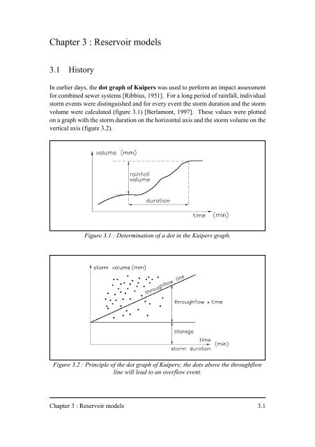
In earlier days, the dot graph of Kuipers was used to perform an impact assessment
for combined sewer systems [Ribbius, 1951]. For a long period of rainfall, individual
storm events were distinguished and for every event the storm duration and the storm
volume were calculated (figure 3.1) [Berlamont, 1997]. These values were plotted
on a graph with the storm duration on the horizontal axis and the storm volume on the
vertical axis (figure 3.2).
Figure 3.1 : Determination of a dot in the Kuipers graph.
Figure 3.2 : Principle of the dot graph of Kuipers; the dots above the throughflow
line will lead to an overflow event.
Chapter 3 : Reservoir models 3.1

In this graph each storm is represented by a dot, but the distinction in individual storms
is rather artificial. Although the rainfall variation is only incorporated in
an approximate way, the importance of a long term approach was already stressed.
In order to determine the number of storms that lead to an overflow event,
the throughflow line is drawn. The throughflow is the outflow from the sewer system
to a treatment plant or to a downstream catchment at the place the subcatchment is
hydraulically disconnected. The throughflow line crosses the vertical axis at a volume
equal to the storage in the combined sewer system and has a slope equal to the
throughflow from the combined sewer system, when a constant (pumped) throughflow
is assumed (figure 3.2). All dots above the throughflow line will lead to an overflow
event. Based on this principle, graphs were made in which the overflow frequency is
presented as a function of the maximum storage in the system and the maximum
throughflow from the system (figure 3.3) [Berlamont, 1990].
Figure 3.3 : Overflow frequency calculated with the ‘dot’ method of Kuipers
for the Uccle rainfall for the period 1958-1968 [Berlamont, 1990].
3.2
The influence of rainfall and model simplification on combined sewer system design

In this figure 3.3 the constant throughflow is presented on the horizontal axis
(in [m 3 /h/ha] for the upper horizontal axis and in [mm/h] for the lower horizontal axis),
while the maximum storage in the system is presented on the vertical axis (in [m 3 /ha]
at the left side and in [mm] at the right sight). The lines from the left top to the right
bottom are the isolines for the overflow frequency (from 2 to 25 p.a.).
The major disadvantage of this ‘dot’ method is the simplification of both rainfall and
model parameters. The method does not take into account the antecedent rainfall nor
the variability of the rainfall within a storm. By linking every storm to only one storm
duration (i.e. the duration of the total storm event), short overflow events for sewer
systems with a smaller critical storm duration may be missed. All this will lead to
an underestimation of the overflow frequency. There is also no criterion used to
distinguish dependent overflow events. Furthermore, the parameters of the combined
sewer system (storage and throughflow) are used as static parameters and are most
often determined very roughly. It can be concluded that the dot graph of Kuipers can
provide a rough estimation of the overflow frequency, but there remains a very high
uncertainty on the results. The advantage of this method is its simplicity and in earlier
days it was the only relevant possibility for the prediction of the overflow frequency.
It is obvious that by using computer technology, better methods can be developed,
while retaining the simplicity of the methodology.
In the early eighties at the Hydraulics Laboratory of the University of Leuven, a single
reservoir modelling system was developed [Berlamont & Smits, 1984a,b,c], which was
later extended to the multiple reservoir modelling system Glas [Glas, 1986; Berlamont
et al., 1987]. Glas is a linear reservoir modelling system, which means that the
throughflow of the reservoir is defined as a linear function of the storage in the
reservoir. Several reservoirs for subcatchments can be connected in series or parallel.
With such a reservoir model the real variability of the rainfall can be included. Also
the antecedent rainfall is included, because the time variation of the storage in the sewer
system is taken into account. The reservoir modelling system Glas used hourly rainfall
data as input for the period 1967-1986 measured at Uccle. This might be too smoothed
as rainfall input, because the rainfall variation within one hour can be high. Because
of the fact that the real succession of the rainfall is taken into account for a long period
(20 years) and a statistical analysis on the results is performed afterwards,
the assessment of the overflow parameters will be much better than using the Kuipers
graph. Using this kind of model, parameters other than the overflow frequency can be
easily determined (statistically), as there are overflow volumes, discharges and
durations. The remaining disadvantage of the Glas modelling system is the assumption
of the linearity between storage and throughflow, which is for many applications not
justified. The major bottleneck in the use of reservoir models is the calibration of the
sewer system parameters. The calibration is a very important stage, which is often
disregarded.
Chapter 3 : Reservoir models 3.3

3.2 Characterisation of sewer systems
3.2.1 Concept
In the past many procedures were used to determine the parameters for simplified
models. This has lead to a distrust in simplified models, because the results were often
not accurate. In this work, special attention is paid to the calibration of the sewer
system parameters. The purpose is to establish a methodology to characterise combined
sewer systems in order to find the necessary parameters for a reservoir model. In order
to be generally applicable in practice, this methodology must be as simple as possible
and unambiguous. This can only be obtained using a physically based approach in
order to find the sewer system parameters.
As the flow in any system has to comply with the continuity equation, this equation will
be the base of the system characterisation. Whereas in the reservoir modelling system
Glas the relationship between storage in the system and the throughflow was prescribed
(assumed to be linear), in this work a methodology will be established to find the real
relationships. This approach can only be used when the inflow into the system and
the throughflow are known. As very limited measurement data on both these aspects
at the same time are available and the accuracy of the measurements is highly
influenced by factors other than the sewer system parameters themselves, it is better to
base this characterisation on simulations with detailed hydrodynamic models. For this
study the hydrodynamic models Spida and Hydroworks (Wallingford Software, UK)
are used, as they are commonly used in Flanders. If a detailed hydrodynamic model is
available for a specific sewer system, the major sewer system parameters can be easily
determined using some single storm simulations. In order to obtain a good calibration,
a wide range of single storm simulations must be used in order to get a complete picture
of the model behaviour. In most cases a detailed hydrodynamic model is available
(e.g. in the framework of the Hydronaut studies), because the sewer system was
designed using detailed hydrodynamic simulations. In this case the hydrodynamic
model is verified and assumed to be as close to reality as possible. Moreover, if long
term hydrodynamic simulations should be performed, this verified hydrodynamic model
would be used anyway. In order to calibrate the simplified model, in the first instance
only the sewer system parameters are taken into account. Therefore, in the
hydrodynamic simulations the runoff model is not considered in this routing calibration
stage.
The calibration procedure is split into three parts. First, the concentration time
is determined. Secondly, the relationships between the storage in the system and
the throughflow are studied. Finally, the runoff module is calibrated. In a first
stage a simple catchment with one downstream throughflow and overflow is
assumed to explain the procedure. Afterwards the extension to more complex
systems is addressed.
3.4
The influence of rainfall and model simplification on combined sewer system design

3.2.2 Concentration time
As was already mentioned in the previous chapters, the concentration time is a very
important parameter in sewer system design. It is one of the basic parameters for the
flow through a sewer system and should therefore be incorporated in the simplified
model. The concentration time at a specific calculation point can be found as the time
between the peak rainfall input and the maximum discharge in the calculation point
(see paragraph 2.1.1). In this way it is also easy to determine the concentration time
using single storm events. The composite storms are peaked, which makes it easy to
determine the differences between the peak in inflow and the peak in outflow. As the
concentration time is different for every pipe or node in the system, the place must be
defined where the concentration time must be determined. For the impact assessment
of combined sewer systems, an optimal prediction of the throughflow and the overflow
discharges is preferred. Therefore, the concentration time is determined as the
difference between the peak of the rainfall input and the peak of the sum of
throughflow and overflow discharges, because this sum is the total outflow from the
system at the downstream end. The whole catchment is assumed as one reservoir for
which only the outflow (i.e. throughflow + overflow) is important. The flow inside all
the individual pipes themselves is not important in this case. Therefore, only the
concentration time for the global outflow is considered.
As the concentration time is the time the water needs to pass through the system and
the flow velocity is to some extent dependent on the magnitude of the flow, it is clear
that the concentration time is not a constant value. For pipe sections with increasing
(or equal) width for increasing height, the velocity is monotonously increasing with the
water depth, just as the flow, but for circular conduits this is not the case [Berlamont,
1997]. However, the velocity is increasing faster than the discharge for low water
depths and the increase is slowing down for larger water depths (figure 3.4).
There is a limitation for the increase in velocity with increasing flow, which is more
rapidly reached for closed sections. When the pipes get pressurised, the velocity is
linearly varying with the flow, while for lower flows the variation of the velocity is
depending on the filling ratio. For a whole network this range of variability will be
phased out, such that the overall relationship between discharge and velocity can be
approximated with a linear relationship. As the concentration time inversely varies
with the velocity, in a first approximation, the concentration time could be assumed to
vary with the inverse of the discharge (hyperbolic function).
For several sewer systems the variation of the concentration time with the flow is
calculated using a wide range of composite storms with frequencies between 20 p.a. till
return periods of 20 years. A typical result is shown in figure 3.5. The concentration
times (obtained as the peak shifts between rainfall and outflow) are presented as
a function of the maximum discharge.
Chapter 3 : Reservoir models 3.5

1.2
U/U full
1
0.8
0.6
circular section
square section
0.4
0.2
0
0 0.2 0.4 0.6 0.8 1 1.2 Q/Q full
Figure 3.4 : Relationship between velocity U and discharge Q
(relative to the velocity U full and the discharge Q full in a completely filled pipe)
in different types of sections.
16
concentration time (min)
14
12
10
8
6
4
2
0
0 0.2 0.4 0.6 0.8 1 1.2 1.4 1.6 1.8 2 2.2
maximum discharge (m 3 /s)
Figure 3.5 : Variation of the concentration time with the peak discharge
for a small (partly steep) gravitary sewer system and a hyperbolic fit to it.
The concentration time is strongly varying for this small sewer system and the variation
can be very well approximated by a hyperbolic function. It can be observed in
figure 3.5 that the decrease in concentration time is limited for larger discharges.
As the available rainfall series has a time step of 10 minutes, an error on the
3.6
The influence of rainfall and model simplification on combined sewer system design

(implemented) concentration time of some minutes is negligible as compared with the
intrinsic smoothing within the rainfall data. For larger systems the variation of the
concentration time will be (relatively) smaller, because the flow is more smoothed. For
more complex and non-linear systems there will often be a larger variability on the
concentration time. This leads to poorer fits of the variation of the concentration time
with the flow. However, from the modelling point of view it is especially important to
predict correctly the lower limit for the concentration time in order to ensure that at
least the shift in peak flows is sufficiently accurate. In cases where no clear peak shift
in the flow can be determined (e.g. when only one single pump is giving a constant
maximum throughflow over a long time), the time of the maximum flow at the end of
the sewer system can be observed taking into account the maximum water level.
The peak flow is then determined as the time of the maximum water level during
the (longest) period that the pump is working. This is an indication of the time for
the maximum discharge that occurs upstream of the pump.
3.2.3 Storage/throughflow-relationships
3.2.3.1 Introduction
The most important parameters of the sewer system are those which describe
the relationship between the state parameter (i.e. the storage volume) and the flow
parameters (i.e overflow discharge and throughflow). When the continuity equation is
applied to the inflow (i.e. composite storms) and the outflow (i.e. the results of
hydrodynamic simulations), the storage volume in the system can be calculated at every
time step. By eliminating the time using the time dependent storage and the outflow
hydrographs, the relationships between storage in the system and throughflow can
be determined. This can be performed for hydrodynamic simulations using a wide
range of single (composite) storm events. This relationship can be easily visualised in
a storage/throughflow-graph (e.g. figure 3.6).
In order to match the proposed reservoir model the rainfall input is first smoothed over
the concentration time before the continuity equation is applied (see paragraph 3.3.1).
As can be seen in figure 3.6 there is a clear relationship between the storage in the
sewer system and the throughflow. However, there is also a clear influence of the input
into the system as well. The storage volume is much larger during the rising branch
than during the falling branch of the storm. This hysteresis effect can be assigned to
the dynamic storage in the system.
It has been checked if this variation is not dependent on the rainfall type using a wide
range of rainfall events. The two extreme types of storms are a constant intensity
during the storm duration corresponding to the IDF-relationships on the one hand and
the peaked composite storms on the other hand. These two storm types were simulated
Chapter 3 : Reservoir models 3.7

for a wide range of return periods in several sewer systems. Some results are shown
in figure 3.7.
14
12
10
8
throughflow (mm/h)
decreasing
rainfall
intensity
f = 1 f = 2
6
4
2
increasing
rainfall
intensity
f = 3 f = 4
f = 5 f = 7
f = 10 f = 14
0
0 0.5 1 1.5 2 2.5 3 3.5 4 4.5 5
storage (mm)
Figure 3.6 : Storage/throughflow-relationship for a small gravitary (partly steep)
sewer system for a range of composite storms with different frequencies f [p.a.].
12
storage in the sewer system (mm)
10
8
6
4
maximum
beginning
end
2
0
0 1 2 3 4 5 6 7 8 9 10 11 12
maximum overflow discharge (mm/h)
Figure 3.7 : Variation of the storage during the overflow event (at the beginning,
at the end and maximum) in two sewer systems ( and —) for a wide range of rainfall
events (constant intensities as well as peaked composite storms).
3.8
The influence of rainfall and model simplification on combined sewer system design

In figure 3.7 the storage in the system at the beginning and at the end of the storm are
shown as well as the maximum storage that occurred. If these storage values are ranked
as a function of the maximum overflow discharge (i.e. approximately the maximum
outflow minus a constant throughflow when the overflow starts spilling), a clear trend
is observed. The storage at the end of the overflow event is an almost constant value.
At this moment the rainfall input into the system is most often nil or very small. In that
case the system behaves as a static reservoir with a fixed volume that is completely full.
The maximum storage in the system appears to be linearly varying with the maximum
discharge. The difference between the maximum storage and the storage at the end of
the event can be assigned to the dynamic storage, which seems to be highly correlated
with the maximum discharge. The fluctuation of the storage at the beginning of the
overflow event is due to the shape of the hyetograph. For peaked storms and (high)
constant rainfall input over short durations the storage at the beginning of the overflow
event will be near to the maximum storage, while for constant rainfall input over longer
durations the storage at the beginning of the overflow event will be more
an intermediate value. This indicates that the dynamic storage is highly dependent on
the instantaneous inflow.
3.2.3.2 Static storage
The maximum static storage is the storage in a sewer system when the system is
filled up to the crest of the weir, when there is no throughflow and the water is
stagnant (figure 3.8).
Figure 3.8 : Longitudinal profile of a sewer system
on which the static storage is indicated (hatched area).
Chapter 3 : Reservoir models 3.9

Although this is an unrealistic (artificial) situation, this state is most often a very good
approximation of the situation at the end of an overflow event (figure 3.7). At least the
maximum static storage in a sewer system can be assessed in this way, even if there is
a flow in the system which creates an extra storage (this is most often the case). In the
same way the static storage at any time can be assessed as the storage during the
emptying of the system when no rainfall input is present. This means that the
instantaneous static storage, for instance for the case of figure 3.6, must be very close
to the storage during the falling branch of the storm (slightly smaller (see figure 3.15)).
In figure 3.7 it can be seen that the storage at the end of the overflow event is a good
indication of the maximum static storage in the system. If only the static storage is
incorporated, the storage at the beginning of the smallest overflow event can also be
a good estimation for the static storage (values near to 0 on the horizontal axis in
figure 3.7). Although the maximum static storage can be easily obtained at the end of
the overflow event, it is important to use the instantaneous relationship between storage
and throughflow for the rising branch of the storm up to the moment the overflow starts
spilling. This is necessary to obtain a good estimation of the start of the overflow.
The primary objective should be to detect if an overflow occurs or not and when it
starts. The emptying of the system after the overflow event only has a second order
effect, because the storage in the system can have an influence on the following
overflow event. This means that in the first instance the dynamic storage can be
neglected. As for sewer system calculations in Flanders the composite storms are used,
it is logical to use the composite storm that will just lead to an overflow event to
determine this storage/throughflow-relationship in a first approach. This first
approach has been applied to a number of different sewer systems and provides already
a lot of information on the sewer systems behaviour. In figure 3.9 the ‘static’
storage/throughflow-relationship is shown for a small sewer system with a gravitary
throughflow.
3.10
The influence of rainfall and model simplification on combined sewer system design

200
175
150
125
100
75
50
25
0
throughflow (l/s)
real relationship
linear 'static' approach
storage (m 3 )
0 20 40 60 80 100 120 140
Figure 3.9 : Storage/throughflow-relationships up to the moment the overflow starts
spilling for a small sewer system with a gravitary throughflow.
It can be seen in figure 3.9 that the relationship between storage and throughflow is
almost linear. In that case the sewer system is labelled as ‘behaving linearly’. As the
throughflow from the system is linearly varying with the volume in the system and the
volume in the system is a function of the inflow through the continuity equation,
a specific input hydrograph will be smoothed, but the antecedent condition in the
reservoir will have only a limited influence. The system behaviour is then driven by
the flow.
In figure 3.10 the ‘static’ storage/throughflow-relationship is given for a small sewer
system with a single pump for the throughflow. It can be seen that the relationship
between storage and throughflow in this system is far from linear. If this relationship
would be approximated with the best linear fit (as is shown in figure 3.10) large errors
on the system behaviour are made. If a linear approximation is made based on the
maximum storage and the maximum throughflow only, the error will be even larger.
This clearly shows that it is not sufficient to determine the maximum storage and
maximum throughflow only, but that the instantaneous relationship between storage
and throughflow is equally important. When the relationship between the storage in the
system and the throughflow is divergent from linearity, the system behaviour is labelled
as non-linear. For this system (figure 3.10), the throughflow is even completely
independent on the storage volume in the system. This means that the throughflow is
hardly influenced by the immediate input into the system, but mainly by the antecedent
rainfall over a longer time. The system behaviour is driven by the volume instead of
the flow. The throughflow (and overflow) hydrograph can be completely different
when the same input hydrograph is used, depending on the antecedent rainfall.
Chapter 3 : Reservoir models 3.11

70
60
50
40
30
20
throughflow (l/s)
bi-linear fitting
linear through maxima
fitted linear
10
0
storage (m 3 )
0 200 400 600 800 1000 1200 1400
Figure 3.10 : Storage/throughflow-relationship for a small sewer system
with a single pump for the throughflow.
The two previous examples are the two most extreme possible behaviours of a sewer
system. In most cases the behaviour is intermediate. In figure 3.11,
the storage/throughflow-relationship is shown for a medium size sewer system with
a complex throughflow relationship (pumping station with five pumps). Although there
are some parts in the relationship which are non-linear, the global effect does not
diverge largely from a linear relationship.
1.2
throughflow (m 3 /s)
1
0.8
0.6
0.4
0.2
0
hydrodynamic
linear reservoir
0 1000 2000 3000 4000 5000 6000 7000
storage (m 3 )
Figure 3.11 : Storage/throughflow-relationship for the sewer system of Dessel
(with 5 pumps in series) for a composite storm which just leads to an overflow event.
3.12
The influence of rainfall and model simplification on combined sewer system design

The influence of the simplifications in the system behaviour, as shown in figure 3.10,
on the effects caused by the composite storm, which has been used to derive the
storage/throughflow-relationship, can be seen in the figures 3.12 and 3.13. If a good
linear approach is fitted, the overflow and throughflow volumes will be approximated
well, but the shape of the hydrographs will be different. Consequently, the type of
rainfall input can significantly influence the outflow. However, it is difficult to specify
what a good linear approximation means. In this work the volume under the
storage/throughflow-relationship is taken equal for both curves (e.g. figures 3.9 to
3.11), which seems to lead to good results. In that case the mean deviation from this
state/flow-relationship is minimised, but it remains an arbitrary choice. If the linear
approximation would only be based on the maximum storage and throughflow as is
shown in figure 3.10, the overflow events will even be larger. These results amplify
the conclusion that not only the maximum system parameters are important,
but that the instantaneous relationship between storage and throughflow is equally
important.
120
overflow discharge (l/s)
100
80
60
40
hydrodynamic model
linear reservoir model
bi-linear reservoir model
20
0
390 420 450 480 510 540
time (min)
Figure 3.12 : Overflow discharge for a single composite storm that will just lead to
an overflow event for a small sewer system with a single pump for the throughflow
(storage/throughflow-relationships in figure 3.10).
Chapter 3 : Reservoir models 3.13

2500
throughflow volume (m 3 )
2000
1500
1000
500
hydrodynamic model
linear reservoir model
bi-linear reservoir model
0
0 240 480 720 960 1200 1440
time (min)
Figure 3.13 : Throughflow volume for a single composite storm that will just lead to
an overflow event in a small sewer system with a single pump for the throughflow
(storage/throughflow-relationships in figure 3.10).
3.2.3.3 Dynamic storage
If the static storage is defined as the storage below a horizontal plane at the crest
level of the overflow, the dynamic storage can be defined as the storage above this
horizontal plane, which is due to the flow in the system (figure 3.14). Although this
is an artificial division, these two components can be recognised in the system
behaviour.
3.14
The influence of rainfall and model simplification on combined sewer system design

Figure 3.14 : Longitudinal profile of a sewer system on which the static
and dynamic storage is indicated using a strict definition of
storage under and above the crest level.
As already mentioned, the maximum dynamic storage is correlated with the maximum
overflow discharge (figure 3.7). Therefore, it could be assumed that there is
a relationship between the instantaneous dynamic storage and the global outflow from
the system (overflow + throughflow). It is more common to link the dynamic storage
to the inflow (e.g. Muskingum method [Cunge, 1969]) than to link it with the overflow
discharge, although the optimum relationship will be a combination of both. If the
inflow hydrograph is first smoothed in the same way as during a hydrodynamic routing,
the instantaneous values of this smoothed hydrograph will be near to the sum of the
instantaneous values of the overflow and the throughflow. This means that the dynamic
storage can be assessed as a function of the smoothed inflow hydrograph. In this work
this smoothing is obtained by an averaging of the runoff over the concentration time as
will be further addressed in paragraph 3.3.1. In figure 3.15 an example is given where
the dynamic storage is included as a linear function of the smoothed inflow. The total
storage can then be obtained by the summation of the static and the dynamic
storage. The correlation between the relationship for the total storage obtained with
a hydrodynamic simulation and those obtained using the linear relationships between
the dynamic storage and inflow on the one hand and between the static storage and the
throughflow on the other hand is very good for this sewer system (figure 3.15).
The incorporation of the dynamic storage can certainly improve the estimation of the
overflows, especially with respect to the overflow duration and the (instantaneous)
overflow discharges, although with only a static storage a good result is already
obtained in many cases. The incorporation of the dynamic storage not only improves
the shape of the overflow events (i.e. the variation of the overflow discharge in time),
it also allows a better approximation of the emptying of the system. The antecedent
rainfall conditions for the next storm will be better incorporated in this way.
Chapter 3 : Reservoir models 3.15

200
175
150
125
100
75
50
25
0
throughflow Q through (m 3 /s)
V d = k dyn * Q in
V s = k stat * Q trough
V tot = V d + V s
real relationship
dynamic storage
static storage V s
total storage V tot
0 20 40 60 80 100 120 140
storage (m 3 )
V d
Figure 3.15 : Linear ‘dynamic’ approach (with slopes k stat and k dyn ) for the
storage/throughflow-relationship of a small gravitary sewer system
(for the composite storm which will just lead to an overflow event).
In order to obtain a good approximation of the relationship between inflow and
dynamic storage, the relationship cannot be fitted only using the composite storm which
will just lead to an overflow event. In that case the range for which the relationship is
valid is too limited. Therefore, it is better that the fitting is performed using the whole
range of composite storms. This increases the calibration efforts, but it can be easily
automated.
Unfortunately, the determination of a dynamic storage is not always that easy as can be
seen in figure 3.16. However, the advantage is that the falling branch is better
described, while the rising branch of the storm is predicted equally well as in the ‘static’
approach. The reason that the fitting in figure 3.16 does not seem to be optimal is due
to the fact that the relationship between inflow and dynamic storage is based on a whole
range of different composite storms. The overall correlation is optimal, but for each
specific storm the differences may be considerable.
3.16
The influence of rainfall and model simplification on combined sewer system design

1.2
throughflow (m 3 /s)
1
0.8
0.6
0.4
0.2
0
hydrodynamic model
dynamic reservoir model
0 1000 2000 3000 4000 5000 6000 7000
storage (m 3 )
Figure 3.16 : Storage/throughflow-relationship for the sewer system
of Dessel when the dynamic storage is included
for a composite storm that will just lead to an overflow event.
3.2.3.4 Extra storage during the overflow event
During the overflow event the water will rise above the crest level. In some cases this
increasing water level can lead to significant extra backwater effects, which results in
increased storage in the system. This storage above the crest level can be defined as
dynamic storage as is shown in figure 3.14, but it is difficult to link this dynamic
storage unambiguously to the inflow as proposed in paragraph 3.2.3.2. Therefore, it
is better to define an extra storage above the crest level as the storage between a
horizontal plane at the crest level and a horizontal plane at the maximum water
level above the crest of the overflow (figure 3.17). In that definition the dynamic
storage is only the part above the horizontal plane at the maximum water level
above the crest of the overflow. Again, this is an artificial division, but these three
components can be recognised in the system behaviour.
This extra (static) storage above the weir can be assumed to be a function of the
overflow discharge. For a free overflow the relationship between discharge Q and
water level h above the crest is a non-linear function [Berlamont, 1996] :
(3.1)
This relationship may be the case for a storage basin (figure 3.18).
Chapter 3 : Reservoir models 3.17

Figure 3.17 : Longitudinal profile of a sewer system on which the static, dynamic
and extra storage during the overflow event are indicated.
1
overflow discharge (m 3 /s)
0.8
0.6
0.4
0.2
0
3000 3030 3060 3090 3120 3150 3180 3210
static storage (m 3 )
Figure 3.18 : Relationship between overflow discharge and volume in the system
for the storage basin in the sewer system of Dessel.
3.18
The influence of rainfall and model simplification on combined sewer system design

Also for combined sewer systems the extra storage (V) available can be limited
(as in figure 3.18), which leads to a similar non-linear relationship (curving in the same
direction as equation (3.1) : Q - V n , with n > 1). On the other hand, also the overflow
discharge Q may be restricted (e.g. by the transport capacity of the pipes from the
overflow structure to the receiving water). In that case a non-linear relationship with
a curving in the other direction (Q - V n , with n < 1) is obtained (figure 3.19).
1.4
overflow discharge (m 3 /s)
1.2
1
0.8
0.6
0.4
0.2
0
T = 1 year
T = 2 year
T = 5 year
T = 10 year
T = 20 year
bi-linear fit
0 2000 4000 6000 8000 10000 12000 14000
static storage (m 3 )
Figure 3.19 : Relationship between storage and overflow discharge for the overflow
in the sewer system of Dessel for design storms with different return periods (T).
Figure 3.19 shows that the extra storage during the overflow event can be large. In this
case this extra storage during the overflow event also has a major effect on the shape
of the overflow hydrograph. In figure 3.20 the effect on the overflow events is shown
for several situations : i.e. caused by a single storm using a static reservoir model only,
using a ‘dynamic’ reservoir model (i.e. reservoir model for which the dynamic storage
is included as a function of the inflow) and incorporating the extra storage during
the overflow event. The influence on the total volume of the overflow event is very
small, but the influence on the shape (discharge, duration) is significant. In figure 3.21,
the effect on some large overflow events is shown for the same sewer system, showing
that the peak discharges and overflow durations will be predicted well for a wide range
of storms. The differences in shape between the overflow events of both models
(figure 3.21) are due to the hysteresis of the extra storage during the overflow event
(figure 3.19).
Chapter 3 : Reservoir models 3.19

1.6
overflow discharge (m 3 /s)
1.4
1.2
1
hydrodynamic model
static reservoir model
dynamic reservoir model
+ storage during overflow
0.8
0.6
0.4
0.2
0
390 400 410 420 430 440 450 460 470 480 490
time (min)
Figure 3.20 : Overflow discharges for the combined sewer system of Dessel
for different models and a composite storm
which will just lead to an overflow event.
1.4
1.2
1
0.8
0.6
0.4
0.2
overflow discharge (m 3 /s)
hydrodynamic model
optimal reservoir model
0
180 210 240 270 300 330 360 390 420 450 480
time (min)
Figure 3.21 : Overflow discharges for the sewer system of Dessel for return periods
between 1 and 20 times p.a. obtained using the hydrodynamic model and the
reservoir model with extra storage above the weir (see figure 3.19).
3.20
The influence of rainfall and model simplification on combined sewer system design

3.2.4 Runoff models
After the calibration of the routing through the sewer system against a verified detailed
hydrodynamic model, the runoff model can be calibrated separately. As the
variability of the rainfall and consequently of the water input into the sewer system is
high, the calibration of the runoff model must be carried out using a wide range of
measurements. The calibration must be performed in such a way that the input volumes
are similar in the model and in the measurements. Most often it is not possible to also
obtain similar instantaneous discharges in model and measurements, because of the
high uncertainty on the parameters. There are significant uncertainties on the rainfall
measurements, on the runoff coefficients, on the losses and on the contributing area.
If the cumulative input is corresponding well in the model and measurements, the errors
on the instantaneous discharges are only of second order importance. An example of
the calibration of a runoff model is given in paragraph 6.5.
A wide range of runoff models can be used. From the modelling point of view the most
extreme runoff models are on the one hand a fixed runoff coefficient and on the other
hand a fixed depression storage (i.e. the storage in depressions on the surface).
Using a fixed runoff coefficient leads to rainfall losses which are a fixed percentage
of the rainfall input. This is a model with a linear behaviour, because the output is
linearly varying with the input. The losses are independent of the antecedent rainfall.
Using a fixed depression storage on the other hand, leads to a non-linear relationship
between in- and outflow. If the depression storage is empty, it will be filled during
the first part of the storm and the shape of the inlet hydrograph might be changed.
If the depression storage is already filled by antecedent rainfall, it will have no
influence on the storm. For this kind of model the antecedent rainfall and the intrinsic
variability of the rainfall are very important.
For continuous simulations the runoff models should not be event based, even if they
are calibrated using single measured events. For that reason a depression storage model
cannot simply be used to subtract the first volume of a storm as is often proposed in
event based models [Van den Herik & Van Luytelaar, 1990; WS, 1996], because of the
subjective definition of a ‘storm’. The depression storage must be written as a function
of instantaneous parameters. This can for instance be performed using a simple
reservoir model for which the outflow is linearly varying with the inflow and with the
depression storage (figure 3.22). The depression storage S is thus limited to S max . If
this relationship is incorporated in the continuity equation and this differential equation
is solved, an exponential filling of the depression storage is obtained :
S
⎡ Vin
= S − ⎛ ⎞ ⎤
max ⎢1 exp⎜−
⎟ ⎥
(3.2)
⎣⎢
⎝ Smax
⎠ ⎦⎥
In equation (3.2), V in is the cumulative inflow into the reservoir.
Chapter 3 : Reservoir models 3.21

Figure 3.22 : Depression storage model.
Using this equation (3.2) for the depression storage model simplifies continuous
simulations, because it is not event based. Moreover, this continuous relationship is
physically more realistic than the storage of the first rainfall volume. However,
the exponential filling has most often no significant influence on the rainfall runoff
as compared for instance with a fixed initial depression storage at the beginning of
a storm. Using this exponential filling of the depression storage, an inflowing rainfall
volume equal to S max will be retained for 63 %.
This kind of non-linear runoff model responds very different from a runoff model using
a fixed runoff coefficient. This can be shown when for the depression storage model
the instantaneous runoff coefficients are calculated. In figure 3.23, the instantaneous
runoff coefficients for a depression storage model are calculated in every (10 minute)
time step of the historical rainfall series of 27 years assuming a maximum depression
storage of 1.5 mm. These instantaneous runoff coefficients are ranked as a function of
the rainfall intensity. For the rainfall intensities that occur several times, the mean
value for the instantaneous runoff coefficients is presented in figure 3.23 by the markers
according to the primary (left) vertical axis. The number of times that a certain rainfall
intensity occurs is presented by the line according to the secondary (right) vertical axis.
Only the mean values per rainfall intensity are shown, but for the low intensities there
is a large variation (using the whole range from 0 to 1).
An extra parameter p (between 0 and 1) could be incorporated to delay the filling of the
depression storage (i = rainfall intensity; Q r = runoff discharge) :
( 1 )
Qr = − p i + p
S
S
max
i
(3.3)
⎡
S S p V in
= − ⎛ ⎞ ⎤
max ⎢1 exp⎜−
⎟ ⎥
(3.4)
⎣⎢
⎝ Smax
⎠ ⎦⎥
3.22
The influence of rainfall and model simplification on combined sewer system design

instantaneous runoff coefficient
1
0.9
number of occurence
2000
1800
0.8
1600
0.7
1400
0.6
1200
0.5
1000
0.4
0.3
instantaneous runoff coefficient
number of occurrence
800
600
0.2
400
0.1
200
0
0
0 1 2 3 4 5 6 7 8 9 10 11 12 13 14
rainfall intensity (mm/h)
Figure 3.23 : Instantaneous runoff coefficients (mean values
for every rainfall intensity) for a depression storage model
with a maximum storage of 1.5 mm (markers) and the
corresponding number of occurrence of the rainfall intensities (line).
In order to make the runoff model continuous, the depression storage must also be
emptied. This can for instance be implemented by applying evaporation.
The evaporation is varying over the year (equation 1.1). The influence of this variation
on the total evaporation volume is however much smaller than the large variation of the
evaporation capacity itself, because of the limited availability of water in the
depressions on the surface. Figure 3.24 shows the monthly evaporated volumes
obtained with a continuous long term simulation of 27 years using different constant
values for the evaporation capacity (full lines) and the effect (bold dashed line) using
a variable evaporation capacity (thin dashed line). The variation of the real evaporation
(i.e. based on the water availability) is much smaller than the evaporation capacity.
For this reason a constant evaporation capacity could be used as an approximation
without having too much effect on the prediction of the overflow events. In the winter
period the evaporation is overestimated if a constant evaporation capacity of 0.1 mm/h
is used, while in the summer this is a good approximation. The overestimation of the
evaporation during the winter is about 10 mm/month. The overflow volumes in winter
could be slightly underestimated in this way. However, most (and most severe)
combined sewer overflows occur in the summer period. Moreover, the evaporation
only influences the antecedent conditions and thus has only a second order effect on the
overflow emissions.
Chapter 3 : Reservoir models 3.23

90
80
70
60
50
40
30
20
10
0
evaporation volume (mm/month)
evaporation capacity
variable evaporation
1 2 3 4 5 6 7 8 9 10 11 12
month of the year
constant
evaporation
(mm/h) :
0.12
0.02
Figure 3.24 : Influence of a constant (full lines) versus a variable evaporation
(bold dashed line) over the year.
If not only impervious areas are modelled, but also pervious areas, then the losses can
also be due to infiltration. Although infiltration is a complex process where many
parameters are involved, a basic model for the infiltration capacity has been proposed
by Horton [1940] :
f = fmin + fmax − fmin exp −k t
(3.5)
( ) ( )
In this formula, f is the infiltration capacity (in [mm/h]), f min and f max respectively
the minimum and maximum infiltration capacity, k the decay factor (in [/h]) and t the
time. The physical meaning of this model is that the infiltration capacity will
exponentially decrease from an initial infiltration capacity f max to a minimum infiltration
capacity f min as the surface becomes wet. Also the restoration of the infiltration capacity
due to the drying-up of the surface can be assumed to occur exponentially :
f = fmax − fmax − fmin exp −k t
(3.6)
( ) ( )
In equation 3.6 a different decay factor k can be used than in equation (3.5).
As for pervious areas the depression storage will be emptied by infiltration, this can be
incorporated in the formula for the depression storage :
⎡ ⎛ Vin
− Fin
⎞ ⎤
S = Smax
⎢1 −exp⎜−
⎟ ⎥
(3.7)
⎣⎢
⎝ Smax
⎠ ⎦⎥
In equation (3.7) F in is the cumulative infiltration. Only if enough water is available in
the depression storage, will the infiltration be equal to the infiltration capacity.
3.24
The influence of rainfall and model simplification on combined sewer system design

Other more detailed runoff models could be used, but the calibration of the parameters
requires large amounts of high quality data. Although a detailed runoff model for the
pervious areas might be necessary for the modelling of runoff to brooks and rivers
(e.g. [Clarke, 1994; DHI, 1993]), the influence of pervious areas and certainly
the influence of the detail of the infiltration description will be small for urban
drainage. If it is necessary to incorporate the infiltration, in most cases the rough
description by Horton (equation 3.5) will suffice.
Next to the losses, also the smoothing by the overland flow should be considered.
Many complex models can be used for this, as was described in paragraph 1.3.3.
However, if this is already taken into account in the single storm simulations that are
used for the calibration of the routing model, the smoothing is already incorporated in
the routing part of the simplified model.
3.2.5 Complex systems
In the previous paragraphs, the sewer system characterisation was applied to simple
sewer systems with one overflow. In reality, sewer systems are more complex, but it
is not always necessary to incorporate this complexity into the model. Before a model
is built, the modeller has to decide which output he wants to obtain. Then, the model
has to be built in such a way that the required output is achieved with the desired
accuracy.
The first step in the transformation of a combined sewer system into a reservoir model
is to separate the hydraulically independent subcatchments. This can be done
e.g. at pumping stations, internal weirs, places where the critical water depth always
occurs, ... The number of places where these conditions occur may be limited.
However, other places can be used to disconnect different subcatchments as long as no
significant backwater effects occur at these places. Whether a certain place is suitable
for disconnecting subcatchments, can be seen in the storage/throughflow-relationships.
If the storage volume in the subcatchment cannot be linked unambiguously to the
inflow and outflow, the place is not suitable for disconnection of subcatchments. In all
other cases the disconnection can be applied at that place.
As a reservoir model is a conceptual model, the outflows of the reservoir do not
necessarily have to agree with the flow in a single pipe or at a single overflow.
The throughflow can be the sum of different pipes which connect two
subcatchments and the overflow can be the sum of two overflows which spill into
the same brook or river. This gives more possibilities to separate subcatchments,
but also to simplify the models.
Chapter 3 : Reservoir models 3.25

When a resulting subcatchment after separation still contains more than one overflow,
the modelling can be performed in several stages. For instance, for a subcatchment
with two overflows two stages are necessary. In the first stage the different overflows
are modelled as one overflow. In the second stage the overflow which starts spilling
first, is modelled together with the throughflow so that only the overflow events of the
second overflow are obtained. The overflow events of the first overflow can then be
obtained by subtracting both overflow series from each other. In figure 3.10
the storage/throughflow-relationship is presented for a catchment with two overflows
and a single pump as throughflow, where the two overflows are modelled together.
In figure 3.25 for the same catchment the storage/throughflow-relationship is given
where the first spilling overflow is modelled as throughflow in order to obtain
the overflow events from the second overflow. This kind of methodology can be
extended to more than two overflows per subcatchment. However, this is a labourious
methodology. It would be easier if these different stages would be implemented
in the reservoir modelling system itself for which a methodology is proposed in
paragraph 3.3.2.
12
11
10
9
8
7
6
5
4
3
2
1
0
throughflow (mm/h)
f = 1 f = 2
f = 3 f = 4
f = 5 f = 6
f = 7 f = 8
0 1 2 3 4 5 6 7 8 9 10 11 12 13
storage (mm)
Figure 3.25 : Storage/throughflow-relationship for the second spilling overflow
in a small sewer system with one pump for the throughflow
for a range of composite storms with different frequencies f
(the discharges of the first spilling overflow are modelled as throughflow).
3.26
The influence of rainfall and model simplification on combined sewer system design

3.3 The reservoir modelling system Remuli
3.3.1 Concept of the modelling system
Based on the basic parameters for combined sewer systems that were identified
in this work, a physically based conceptual modelling system was developed.
This modelling system contains four main parts which are connected in series
(figure 3.26) : a runoff module, a smoothing module, a module for the dynamic storage
and a module for the static storage. The long term simulations can be performed with
rainfall with a time step of 10 minutes at Uccle for the period 1967-1993.
Figure 3.26 : Schematic representation of the reservoir modelling system Remuli.
The runoff module incorporates the rainfall losses and consequently the rainfall input
into the system. In the runoff module a distinction can be made between impervious
and pervious area. For the impervious areas, a fixed runoff coefficient can be specified
as well as a depression storage (i.e. surface storage). The depression storage is filled
exponentially in time as described in paragraph 3.2.4, also including an extra parameter
to delay the filling up of the depression storage (equation 3.4). For the pervious areas,
Chapter 3 : Reservoir models 3.27

the same parameters can be specified as for the impervious areas and as an extra
possibility the infiltration can be modelled using the Horton equation as described in
paragraph 3.2.4. The decay factors for surface wetting (equation 3.5) and drying
(equation 3.6) may be chosen differently. The depression storage on the impervious
areas can be emptied during dry weather using a constant evaporation. The possible
evaporation is strongly influenced by other climatic parameters as for instance
the temperature. However, the actual evaporation from impervious areas varies much
less, because of the limited amounts of water available in the depression storage
(figure 3.24). The evaporation has only a small effect on the losses and does not
influence the prediction of overflows directly. It only slightly influences the antecedent
conditions. Therefore, it is acceptable to use a constant evaporation for emission
predictions at combined sewer overflows. For the pervious areas the depression storage
can also be emptied by infiltration.
In the reservoir modelling system Glas, hourly rainfall was used which already
incorporated some smoothing. Furthermore, a time shift of one or more hours (multiple
of the time step) could be applied on the throughflow. This is sufficient if no better
accuracy than hourly based results is necessary and for sewer systems which have
concentration times of maximum a few hours. Larger concentration times seldom
occured, because in earlier times only small systems were modelled with a single
reservoir. Since 10 minute rainfall data are available now, it is possible to predict the
combined sewer overflows with higher accuracy. In order to obtain the smoothing of
the hydrograph and the time delay of the peak flow, it is necessary to add an extra
smoothing module in the reservoir modelling system. This smoothing is applied to the
runoff.
The smoothing module contains an averaging of the runoff over the concentration time.
In this way the peak shift between inflow and outflow are well determined and part of
the smoothing due to the flow in the system is already incorporated. This smoothing
is necessary, because a single reservoir model has an instantaneous (exponential)
response. This means that the peak shift cannot be predicted well in the reservoir
model, when no extra module for this is included. For the same reason (i.e. exponential
response) a single linear reservoir is not a good tool for this smoothing. If the
concentration time is used as a variable parameter (as a (hyperbolic) function of the
runoff), discontinuities may occur for low concentration times using only multiples of
the 10 minute time step. Therefore the concentration time is incorporated with a higher
accuracy of 1 minute, however without reducing the simulation time step. This also
allows a more accurate smoothing for small systems using a constant concentration
time. The use of the relationship between peak shift and maximum runoff as described
in paragraph 3.2.2 can be generalised for the smoothing of all runoff discharges (not
just only the peaks) in order to obtain continuous smoothing. This is physically
acceptable and has so far led to good results. However, already good results are often
obtained with a constant concentration time which is equal to the peak shift between
rainfall and outflow for the (composite) storm that will just lead to an overflow event.
3.28
The influence of rainfall and model simplification on combined sewer system design

If the concentration time is not taken into account as a variable parameter with
the runoff, the extra variation in smoothing and peak shift can be modelled using
the dynamic storage. In that way the smoothing module and the dynamic storage
module overlap to some extent, although they cannot replace each other completely.
The differential equation that describes a linear static reservoir model is :
dV
dt
= Q − Q
(3.8)
in
through
with :
Q
through
V
=
V
Q m
(3.9)
m
In this set of equations, V is the instantaneous storage volume in the reservoir,
V m the maximum storage, Q in the inflow, Q m the maximum throughflow and
Q out the instantaneous throughflow. The analytical solution for this set of equations
at time t+dt as a function of the instantaneous storage V t in the previous time step t is :
V Q V ⎛
m
Qm
Q
V dt V Qm
t+ dt = in − ⎛ ⎞⎞
⎜−
⎟
⎜
t
V
dt
m ⎝ ⎝ m ⎠
⎟
+ ⎛ ⎞
1 exp exp ⎜−
⎟ (3.10)
⎠
⎝ m ⎠
When the maximum storage V m is reached, the overflow starts spilling and the overflow
discharge is equal to the difference between inflow Q in and maximum throughflow Q m .
The reservoir modelling system Remuli however uses piecewise linear relationships for
the storage/throughflow relationships, which also makes the inclusion of extra storage
during the overflow event possible (see paragraph 3.3.2).
The dynamic storage and the static storage are fitted together as shown in figure 3.15
using the following equations :
Vm
V k Q k Q
Q Q Vdm
= stat through + dyn in = through +
Q
Q in
(3.11)
in which V dm is the maximum dynamic storage corresponding with the maximum
inflow Q dm .
Combined with the continuity equation this leads to :
Or solved :
dV
dt
⎛ Vdm
V
Vt+ dt = Qin
⎜ +
⎝ Q Q
dm
⎛ Vdm
Qm
⎞ Qm
= Qin
⎜1 + ⎟ −
⎝ Q V ⎠ V
V
(3.12)
m
m
dm
m
m
m
⎞ ⎛ Qm
V dt V Qm
⎟ − ⎛ ⎞⎞
⎜−
⎟
t
⎠
⎜
⎝
V
dt
⎝
m ⎠
⎟ + ⎛ − ⎞
1 exp exp ⎜ ⎟ (3.13)
⎠ ⎝ m ⎠
dm
Chapter 3 : Reservoir models 3.29

In the reservoir modelling system Remuli up to 10 reservoirs can be connected in series
or parallel, each with one throughflow and one overflow. Although in the current
version the number of reservoirs is limited to 10, this can be increased without any
problem. An example is shown in figure 3.27. Each of these reservoirs contains the
four modules which are shown in figure 3.26 (eventually the dynamic storage can be
0 and only three modules are then present).
Figure 3.27 : Schematic view of the simplified model for the sewer system of Dessel;
each reservoir contains (part of) the modules in figure 3.26.
3.3.2 Piecewise linear relationships
As the instantaneous relationship between storage and throughflow is important, models
should be built that can take into account a possible non-linear behaviour of the
system. However, most existing modelling systems assume a fixed type relationship
between storage and throughflow (most often a linear relationship or a constant
throughflow). When the parameters of such models are well calibrated, they can
provide a rough estimation of the effects, but the results will not always be accurate.
Therefore, it is better to use modelling systems that do not prescribe the model
structure, but allow a wide range of possibilities. This can be achieved using a
piecewise linear (also named multi-linear) relationship between storage and
throughflow. With this model structure every possible relationship can easily be
approximated by a combination of several successive linear parts. The only restriction
is that the throughflow must monotonously increase with increasing storage.
An example for the ‘static’ modelling approach is shown in figure 3.28.
3.30
The influence of rainfall and model simplification on combined sewer system design

200
throughflow Q (l/s)
175
real relationship
150
125
Q 1
'static' approach
Q = Q 1 +
k 2 * (V-V 1 )
100
75
50
Q = k 1 * V
25
0
0 20 40 60 80 100 120 140
storage V (m 3 )
V 1
Figure 3.28 : Bi-linear ‘static’ approach (with slopes k 1 and k 2 ) for the
storage/throughflow-relationship of a small gravitary sewer system
(for the composite storm which will just lead to an overflow event).
If a linear relationship is used between the volume in the system and the inflow and
outflow, the differential equation (3.12) can be solved analytically (equation 3.13).
This has the advantage that a very fast and accurate calculation can be performed.
Calculation time and accuracy are both very important for long term simulations.
Using the piecewise linear relationships between storage and flow, these advantages
can be retained by applying the analytical solution in a subcoordinate system. The
transition from one linear relationship to another is made by a translation of the
coordinate system (figure 3.29). However, if the starting points of every linear
subrelationship between static storage and throughflow on the one hand and between
dynamic storage and inflow on the other hand are not situated at the same storage
values, the combined analytical solution of static and dynamic storage (equations 3.11
and 3.13) cannot be used anymore. Both relationships must be linear at the same time
in a subcoordinate system. Therefore, it is chosen to uncouple the dynamic storage
from the static storage module as shown in figure 3.26.
Chapter 3 : Reservoir models 3.31

Figure 3.29 : Coordinate system used in the reservoir modelling system Remuli.
This piecewise linear approach with a translation of the coordinate system also allows
the incorporation of extra storage during the overflow event.
The overflow can be modelled as one of the outflows, so that the total outflow Q out
becomes :
V
Q Q Q
( )
V Q V
V Q Q Q V
out = through + over = m + mo = m + mo
(3.14)
V
Q
through
m
where Q m and Q mo are the maximum throughflow and maximum overflow respectively.
Consequently both flows can be found as :
Qm
V V Qm
= =
Q + Q Q
m
m
m
mo
out
m
(3.15)
Q
over
Qmo
V V Qmo
= =
Q + Q Q
m
m
mo
out
(3.16)
This approach of modelling different outflows from one reservoir using different linear
relationships can be extended to more than two outflows. This makes it possible to
handle more complex models where one reservoir can have more than one overflow.
In this way it is not necessary to split up every sewer system into different reservoirs
each with one overflow, nor is it necessary to perform the modelling of subcatchments
with more than one overflow in several stages. These reservoirs with more than one
overflow are not implemented yet, but it can be performed easily.
3.32
The influence of rainfall and model simplification on combined sewer system design

3.3.3 Other features
The reservoir modelling system Remuli is a Fortran 90 coded software program,
which is compiled into an executable file. The interface for the input and output is
an Excel-sheet using macro’s in Visual Basic. The reservoir modelling system Remuli
has an online manual, which is a file in html-format. This manual is included in
appendix B.1. More details on the possibilities can be found in this manual.
Simulations can be performed with single storms, i.e. composite storms as well as user
defined rainfall series. More important are the long term simulations, which can be
performed for the Uccle rainfall with a time step of 10 minutes for the period
1967-1993. In the future this rainfall period can be extended. It is also possible to
select short rainfall series from this historical rainfall series with the reservoir
modelling system as will be described in paragraph 4.3.
Reservoirs can be connected in series and parallel, not only via the throughflow,
but also via the overflow. This means that off-line storage basins in treatment plants
and at overflows can be modelled. Also the modelling of return pumps is
implemented. Return pumps can be used to empty a reservoir after a storm or can also
represent the flow through a flap valve. This type of connection can be used if the flow
is not determined by the reservoir from which the water is pumped, but by the volume
V in the reservoir where the water is pumped into. This is incorporated in the
continuity equation of the receiving reservoir :
dV
dt
= Qin + Qp − Qthrough
(3.17)
Q
p
V
= Qpm
−
V
Q pm
(3.18)
m
The relationship for the pumped discharge Q p (Q pm is the maximum pump capacity)
can be piecewise linear, using the ranges of storage of the reservoir in which the water
is pumped. The pumped discharge has to decrease monotonously with increasing
storage in the receiving reservoir. For every time step it is checked if the volume
that can be pumped is available in the reservoir where the water is pumped from.
Using the possibilities on the modelling of reservoirs and return pumps even the
hydraulic behaviour of a treatment plant can be modelled as is shown in figure 3.30
for the sewer system and treatment plant of Dessel. The modelling of very complex
systems becomes possible, but it is rarely necessary to model it in such a detailed way.
The extremely simplified model in figure 3.27 for the same system already gives very
good results.
Chapter 3 : Reservoir models 3.33

Figure 3.30 : Schematic representation of the reservoir model
for the sewer system and treatment plant of Dessel.
3.34
The influence of rainfall and model simplification on combined sewer system design

For emission modelling it is very important to obtain the results in a statistically
processed way. It would require too much disk space and writing time to write all
results at every time step into a file. The user can choose to write the time step results
for one year into a file, but it is more important to obtain processed results. Therefore,
the overflow events are individually written to a file using parameters as starting time,
duration, overflow volume, mean overflow discharge and peak discharge (during the
time step, i.e. 10 minutes). The overflow ‘events’ can be defined as individual events
or as days with an overflow event. Average values per year, per month (over all the
years) and for the whole simulation are given. To obtain a rough estimation of the
deviation on the results the 68 %-intervals are also given. The peak overflow
discharges seem to fit very well to a lognormal distribution. The overflow volumes and
durations seem to tend more to an exponential distribution. This check for the type of
distribution for the overflow parameters was only carried out on a limited number of
time series and cannot be generalised. Furthermore, there could be a possible effect of
the definition of an overflow event on the distributions for the overflow volumes and
durations. When this statistical information will be used, further research on the type
of distributions should be performed. Finally, a file with the volume balance is written
in order to check the total volumes that have passed the reservoirs. In appendix B.2
some examples of results are shown.
Chapter 3 : Reservoir models 3.35

3.4 Sensitivity analysis
The main sewer system characteristics can be easily implemented in a reservoir model
and the effect can be assessed on the long term. This makes a reservoir model
an excellent tool to perform sensitivity analyses on the parameters and to search for
optimised parameters. The main parameters that can have an influence on the
conception of a sewer system are the throughflow capacity and the storage in the sewer
system. Therefore, graphs can be made on which the overflow parameters are
represented as a function of these two parameters. As demonstrated in the previous
paragraphs, not only the maximum throughflow and storage are important, but also
the instantaneous relationship between both. Therefore, the two most extreme
instantaneous relationships are investigated, as there are the linear relationship and
the constant throughflow. All other relationships are situated somewhere in between.
Another important sewer system parameter is the concentration time. This parameter
influences the peak shift and the smoothing of the hydrographs, so that it can also
strongly influence the overflow parameters. Therefore, this analysis is also performed
for different concentration times. In this analysis no dynamic storage or storage above
the weir is included, as these parameters often only influence the shape of the overflow
events. Finally, the runoff model can influence the results. For this analysis a runoff
model with a depression storage of 2 mm and a constant evaporation of 0.1 mm/h is
assumed. The studied overflow parameters are mainly overflow frequency and volume,
but also overflow durations, mean and peak overflow discharge. The rainfall input used
is the historical series of Uccle for the period 1967-1993.
In figure 3.31 the overflow frequency is visualised for a wide range of possible values
for the maximum storage in a sewer system and the maximum throughflow from the
system, using a linear relationship between instantaneous storage and throughflow.
In the graphs the maximum throughflow is not presented on the horizontal axis, but the
overcapacity. The overcapacity is the maximum throughflow minus the dry weather
flow. In this way these graphs can be used independently of the dry weather flow.
Both maximum storage and overcapacity are presented relative to the contributing area,
so that the graphs are representative for any size of catchment. In figure 3.32
the overflow frequency is visualised using a constant relationship between storage and
overcapacity. In both figures 3.31 and 3.32 a concentration time of 60 minutes is used.
It can be seen from these figures that the type of relationship between storage and
throughflow has a large influence on the predicted overflow frequency. In these graphs
the overflow frequency is defined as the number of days with an overflow event. If the
overcapacity is low, the overflow frequency is strongly influenced by the maximum
storage in the system. Or the other way around, to achieve a specific overflow
frequency much more storage is necessary at low overcapacities. Analogously, graphs
can be made for the percentage of rain water that is spilled via the overflows as is
shown in the figures 3.33 and 3.34.
3.36
The influence of rainfall and model simplification on combined sewer system design

Figure 3.31 : Overflow frequencies calculated with a single linear reservoir model
(concentration time = 60 minutes).
Chapter 3 : Reservoir models 3.37

Figure 3.32 : Overflow frequencies calculated with a single reservoir model
with a constant throughflow (concentration time = 60 minutes).
3.38
The influence of rainfall and model simplification on combined sewer system design

Figure 3.33 : Overflow volumes (% of total rainfall volume) calculated with a single
linear reservoir model (concentration time = 60 minutes).
Chapter 3 : Reservoir models 3.39

Figure 3.34 : Overflow volumes (% of total rainfall volume) calculated with a single
reservoir model with a constant throughflow (concentration time = 60 minutes).
3.40
The influence of rainfall and model simplification on combined sewer system design

Not only the storage, the throughflow and the relationship between these two
parameters, but also the concentration time can have a large influence on the predicted
overflow parameters. In figure 3.36 the effect of the concentration time on the
overflow frequency is shown. For small overcapacities (which is mostly the case) this
effect is however limited.
Other parameters could influence the prediction of the overflow parameters as there are
the runoff model and the used rainfall series (location, time step, measurement period).
Furthermore, the definition of an overflow event can have a large influence, not only
on the overflow frequency, but also on other parameters. This shows that there is still
room for other sensitivity analyses than the ones which are shown here. In this way not
only the sensitivity of the sewer system parameters can be tested, but also the feasibility
of emission criteria.
If a system is obtained with a storage/throughflow-relationship somewhere between
a linear and a constant throughflow, these graphs (figures 3.31 till 3.34) can still be
used to estimate the range in which the overflow parameters are situated. The ‘linear’
and ‘constant’ relationships (dashed lines) which bound the real relationship (solid line)
will also lead to the bounds for the overflow parameters (figure 3.35). In this context
it is important to remark that also the concentration time can have a large influence,
which should be taken into account (e.g. via figure 3.36).
These graphs, in which the overflow frequency is given as a function of the storage
in the system and the overcapacity, provide the same information as the graph of
Kuipers (see paragraph 3.1) These graphs are however much more accurate, because
the rainfall input has not been simplified in this methodology. For that reason the graph
of Kuipers should not be used anymore. Instead the figures 3.31 to 3.34 can be used
and these graphs have therefore been incorporated in the Flemish guidelines [VMM,
1996].
Figure 3.35 : Linear and constant approximations (dashed lines)
for the storage/throughflow-relationship that leads to the bounds
for the overflow parameters.
Chapter 3 : Reservoir models 3.41

Figure 3.36 : Influence of the concentration time on the overflow frequency
for a linear reservoir model for overflow frequencies
of 1, 2, 3, 5, 7, 10, 14 and 20 times p.a.
3.42
The influence of rainfall and model simplification on combined sewer system design

As the overflow events are strongly variable, distributions for all overflow
parameters are obtained. These distributions can be presented as a function of the
mean overflow frequency (over 27 years). The mean overflow frequency is defined
here as the number of days per year with an overflow event. In figure 3.37 the mean
overflow volume per day with overflow is shown as well as the upper limit of the 68 %
two sided confidence interval. From this figure it can be concluded that, except for
very low overflow frequencies, the mean overflow volume per day with an overflow
event is about 4 mm. However, there is a large scatter on the distribution. In figure
3.38 the variation of the mean overflow discharges with the mean overflow frequency
are shown. For higher mean overflow frequencies the mean overflow discharge will
decrease. This is mainly due to the fact that the mean overflow duration also increases
with increasing mean overflow frequency (figure 3.39). The variation of the maximum
overflow discharge within 10 minutes with the mean overflow frequency is similar to
the variation of the mean overflow discharge, but about 60 % higher (figure 3.40).
This comparison as a function of the overflow frequency shows that if the frequency
decreases only small and less severe overflow events will be avoided.
10
9
8
7
6
5
4
3
2
1
0
overflow volume (mm)
0 5 10 15 20 25 30
overflow frequency (days/year)
Figure 3.37 : Mean overflow volume per day with overflow and
the upper limit of the 68 % two sided confidence interval
as a function of the mean overflow frequency.
Chapter 3 : Reservoir models 3.43

9
mean overflow discharge (mm/h)
8
7
6
5
4
3
2
1
0
0 5 10 15 20 25 30
overflow frequency (days/year)
Figure 3.38 : Mean overflow discharge per day with overflow and
the upper limit of the 68 % two sided confidence interval
as a function of the mean overflow frequency.
200
180
160
140
120
100
80
60
40
20
0
overflow duration (min)
0 5 10 15 20 25 30
overflow frequency (days/year)
Figure 3.39 : Mean overflow duration per day with overflow and
the upper limit of the 68 % two sided confidence interval
as a function of the mean overflow frequency.
3.44
The influence of rainfall and model simplification on combined sewer system design

16
peak overflow discharge (mm/h)
14
12
10
8
6
4
2
0
0 5 10 15 20 25 30
overflow frequency (days/year)
Figure 3.40 : Peak overflow discharge (averaged over 10 minutes) per day with
overflow and the upper limit of the 68 % two sided confidence interval
as a function of the mean overflow frequency.
Chapter 3 : Reservoir models 3.45

3.5 Conclusions
In this chapter a methodology has been proposed to identify the most important
sewer system characteristics in order to calibrate a simplified conceptual sewer
model. It is very important that this sewer system characterisation is carried out
on a physical base, so that the obtained parameters have a physical meaning. This is
the key to an accurate model calibration. The major parameters for an emission model
are the storage in the sewer system, the throughflow and the concentration time.
The runoff model also has an important influence in order to obtain a good estimation
of the input into the sewer system model. The results of the sewer system
characterisation have been used to set-up a new reservoir modelling system, named
Remuli. Especially for the relationship between storage and throughflow, it is
important that the model structure is flexible. This is obtained by the implementation
of the piecewise linear relationships. However, this flexibility does not put a heavy
burden on the calculation times, because of the choice for a linear model which can be
solved analytically. The implementation of this analytical solution of the differential
equation and an optimal algorithm for the programming of the computational core have
led to very low calculation times. Compared with hydrodynamic simulations,
the calculation times are 10 4 to 10 6 times smaller using the reservoir modelling system
Remuli. This means that in a single reservoir the historical time series of 27 years can
be simulated within 5 to 15 seconds on a Pentium II 233 MHz computer, depending on
the complexity of the model. Thanks to this fast calculation, this reservoir modelling
system is an ideal tool for sensitivity and scenario analyses, the optimisation of storage,
the calibration of a runoff model, etc... In the near future the reservoir modelling
system Remuli will be extended with water quality modules in a conceptual way and
physically based on the same level as the water quantity aspects. However, this is
beyond the scope of this study. In chapter 6, more attention will be paid to model
verification and the practical applicability of simplified models.
3.46
The influence of rainfall and model simplification on combined sewer system design