Comparison of Angle-only Filtering Algorithms in 3D using Cartesian ...
Comparison of Angle-only Filtering Algorithms in 3D using Cartesian ...
Comparison of Angle-only Filtering Algorithms in 3D using Cartesian ...

You also want an ePaper? Increase the reach of your titles
YUMPU automatically turns print PDFs into web optimized ePapers that Google loves.
where<br />
⎡<br />
v(φ) =<br />
⎢<br />
⎣<br />
0<br />
0<br />
0<br />
β<br />
ɛ<br />
1/r<br />
⎤<br />
+ 1<br />
⎥ r<br />
⎦<br />
[ A(β, ɛ)<br />
0 3<br />
] ⎡ ⎣<br />
s cos γ s<strong>in</strong> α − ẋ o 1<br />
s cos γ cos α − ẏ o 1<br />
s s<strong>in</strong> γ − ż o 1<br />
(47)<br />
The <strong>in</strong>tegrals (45) and (46) can be evaluated over all variables<br />
except for the range r. Integration over r can be done<br />
numerically us<strong>in</strong>g, for example, Monte Carlo approximation.<br />
Due to lack <strong>of</strong> space, the expressions the components <strong>of</strong> ˆξ 1<br />
and P 1 are not presented <strong>in</strong> the paper but can be found <strong>in</strong><br />
[29].<br />
VI. NONLINEAR FILTERING USING RELATIVE CARTESIAN<br />
COORDINATES<br />
The dynamic model (NCVM <strong>in</strong> <strong>3D</strong>) is l<strong>in</strong>ear and the<br />
measurement model for bear<strong>in</strong>g and elevation is nonl<strong>in</strong>ear for<br />
this case.<br />
The widely used EKF is based on l<strong>in</strong>earized approximations<br />
to nonl<strong>in</strong>ear dynamic and/or measurement models [8], [14].<br />
For this case, the l<strong>in</strong>earized approximation is performed <strong>in</strong><br />
the measurement update step. The details <strong>of</strong> the algorithm are<br />
described <strong>in</strong> [8], [14].<br />
The UKF, like the EKF, is also an approximate filter<strong>in</strong>g<br />
algorithm. However, <strong>in</strong>stead <strong>of</strong> us<strong>in</strong>g the l<strong>in</strong>earized approximation,<br />
the UKF uses the unscented transformation (UT) to<br />
approximate the moments [23], [24]. This approach has two<br />
advantages over l<strong>in</strong>earization: it avoids the need to calculate<br />
the Jacobian and it provides a more accurate approximation.<br />
The details <strong>of</strong> the UKF algorithm are described <strong>in</strong> [23], [24]<br />
and [32].<br />
Particle filters are a class <strong>of</strong> sequential Monte Carlo methods<br />
for approximat<strong>in</strong>g the posterior density <strong>of</strong> the target state.<br />
The most common form <strong>of</strong> PF adopts a sequential importance<br />
sampl<strong>in</strong>g (SIS) [15], [6], [32] approach <strong>in</strong> which samples <strong>of</strong><br />
the target state are drawn from an importance density and<br />
weighted appropriately each time a measurement is acquired.<br />
We use a regularised bootstrap filter (BF). This <strong>in</strong>volves first<br />
draw<strong>in</strong>g samples from the prior and weight<strong>in</strong>g the samples<br />
by their likelihood [6], [15], [32]. Regularization is then<br />
performed, as suggested <strong>in</strong> [20], [30], by draw<strong>in</strong>g from a<br />
kernel density approximation us<strong>in</strong>g a Gaussian kernel with<br />
covariance matrix<br />
⎤<br />
⎦ .<br />
VII. NONLINEAR FILTERING USING MSC<br />
The dynamic model us<strong>in</strong>g MSC is nonl<strong>in</strong>ear as <strong>in</strong> (27) or<br />
(28). In addition, the process noise is not additive. S<strong>in</strong>ce,<br />
the bear<strong>in</strong>g and elevation are elements <strong>of</strong> the MSC, the<br />
measurement model (32) is l<strong>in</strong>ear.<br />
The EKF us<strong>in</strong>g MSC is described by Algorithm 1. We note<br />
that l<strong>in</strong>earization <strong>of</strong> the dynamic model is performed over<br />
both the previous state ξ k−1 and the process noise w t k−1 .<br />
As a result, the Jacobian B is a 6 × 12 matrix rather than<br />
the 6 × 6 matrix which would result if the dynamic model<br />
were nonl<strong>in</strong>ear <strong>in</strong> the previous state and l<strong>in</strong>ear <strong>in</strong> the additive<br />
process noise.<br />
A recursion <strong>of</strong> the UKF us<strong>in</strong>g MSC is given by Algorithm<br />
2. In Algorithm 2, the nonl<strong>in</strong>ear transformation is applied to a<br />
12-dimensional random variable. Therefore, 2 × 12 + 1 = 25<br />
sigma po<strong>in</strong>ts are required. The weights are selected as w 0 =<br />
κ/(12 + κ) and w i = 1/[2(12 + κ)], i = 1, . . . , 24 with κ =<br />
−3.<br />
Algorithm 3 presents a recursions <strong>of</strong> the PF us<strong>in</strong>g MSC.<br />
This PF provides state estimates <strong>in</strong> relative <strong>Cartesian</strong> coord<strong>in</strong>ates<br />
by transform<strong>in</strong>g each sample from MSC to relative<br />
<strong>Cartesian</strong> coord<strong>in</strong>ates and comput<strong>in</strong>g the weighted mean.<br />
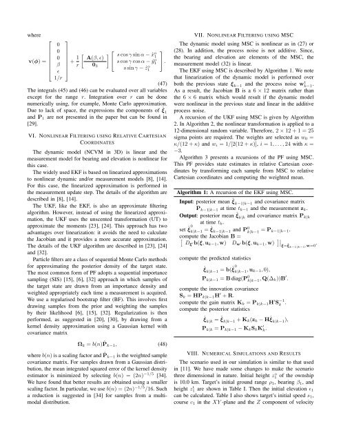
Algorithm 1: A recursion <strong>of</strong> the EKF us<strong>in</strong>g MSC.<br />
Input: posterior mean ˆξ k−1|k−1 and covariance matrix<br />
P k−1|k−1 at time t k−1 and the measurement z k .<br />
Output: posterior mean ˆξ k|k and covariance matrix P k|k<br />
at time t k .<br />
set ˆξ 0 k|k−1 = ˆξ k−1|k−1 and P 0 k|k−1 = P k−1|k−1.<br />
compute the Jacobian B =<br />
[<br />
Dξ ′b(ξ, u k−1 , w) D w ′b(ξ, u k−1 , w) ]∣ ∣<br />
ξ=ˆξk−1|k−1 ,w=0 .<br />
compute the predicted statistics<br />
ˆξ k|k−1 = b(ˆξ 0 k|k−1, u k−1 , 0),<br />
P k|k−1 = B diag(P 0 k|k−1 , Q(∆ k))B ′ .<br />
compute the <strong>in</strong>novation covariance<br />
S k = HP k|k−1 H ′ + R.<br />
compute the ga<strong>in</strong> matrix K k = P k|k−1 H ′ S −1<br />
k .<br />
compute the posterior statistics<br />
ˆξ k|k = ˆξ k|k−1 + K k (z k − Hˆξ k|k−1 ),<br />
P k|k = P k|k−1 − K k S k K ′ k.<br />
Ω k = b(n) ˆP k−1 , (48)<br />
where b(n) is a scal<strong>in</strong>g factor and ˆP k−1 is the weighted sample<br />
covariance matrix. For samples drawn from a Gaussian distribution,<br />
the mean <strong>in</strong>tegrated squared error <strong>of</strong> the kernel density<br />
estimator is m<strong>in</strong>imized by select<strong>in</strong>g b(n) = (2n) −1/5 [34].<br />
We have found that better results are obta<strong>in</strong>ed us<strong>in</strong>g a smaller<br />
scal<strong>in</strong>g factor. In particular, we use b(n) = (2n) −1/5 /16. Such<br />
a reduction is suggested <strong>in</strong> [34] for samples from a multimodal<br />
distribution.<br />
VIII. NUMERICAL SIMULATIONS AND RESULTS<br />
The scenario used <strong>in</strong> our simulation is similar to that used<br />
<strong>in</strong> [11]. We have made some changes to make the scenario<br />
three dimensional <strong>in</strong> nature. Initial height z o 1 <strong>of</strong> the ownship<br />
is 10.0 km. Target’s <strong>in</strong>itial ground range ρ 1 , bear<strong>in</strong>g β 1 , and<br />
height z t 1 are shown <strong>in</strong> Table I. Then the <strong>in</strong>itial elevation ɛ 1<br />
can be calculated. Table I also shows target’s <strong>in</strong>itial speed s 1 ,<br />
course c 1 <strong>in</strong> the XY -plane and the Z component <strong>of</strong> velocity