Positive relationship between non-native and native squirrels in an ...

Pagination not final/Pagination non finale
4 Can. J. Zool. Vol. 86, 2008
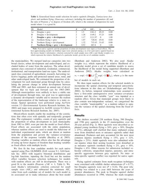
Table 1. Generalized linear model selection for native squirrels (Douglas, Tamiasciurus douglasii,
and northern flying, Glaucomys sabrinus), including the number of parameters (K) and
the ratio of Pearson 2 to degrees of freedom (df), which is the estimate of dispersion for each
model where 1 is a good fit.
ID Model K 2 /df AIC c i w i
1a Douglas = grey 2 1.5 1161.2 49.23 0.00
B Douglas = development 2 1.26 1149.2 37.23 0.00
C Douglas = grey + development 3 1.17 1111.97 0 1.00
2a Northern flying = grey 2 1.07 728.81 45.01 0.00
B Northern flying = development 2 1.32 715.43 31.63 0.00
C Northern flying = grey + development 3 0.92 683.8 0 1.00
Note: Non-native squirrels and the proportion of urban development were input as fixed effects. The
best approximating models (in boldface type) were selected among a to d for each native squirrel based on
the lowest Akaike’s information criterion corrected for small sample sizes (AIC c ) and Akaike weights (w i ),
which represent the relative likelihood of a particular model, given the set of candidate models.
the municipalities. We merged land-use categories into two
broad classes, urban development and undeveloped, and excluded
bodies of water from the analyses. The urban development
class consisted of industrial, residential, commercial,
institutional, and transportation land-use types. The undeveloped
class consisted of agricultural, research, harvesting (selective
logging), parks and protected natural areas, rural, and
other undeveloped lands. We estimated the proportion of development
for each municipal group through time by calculating
the percent change in urban development between
1996 and 2001, and then estimated an annual rate of development
that we back and forward cast for 1983–2003.
Although municipalities were unlikely to have a stable rate
of development through time, our goal was to approximate
a dynamic development variable and to increase the realism
of the representation of the landscape relative to a static estimate.
Spatial operations were performed using ArcView
version 3.3 (Environmental Systems Research Institute, Inc.
2002) and maps were prepared in ArcGIS version 9.2 (Environmental
Systems Research Institute, Inc. 2007).
Mixed-effects models enable the modeling of the correlations
that often exist with spatially and temporally grouped
data. The explanatory variables, counts of grey squirrels and
the proportion of urban development in each municipality
from 1983 to 2003, were put into the model as fixed effects.
Fixed effects are associated with the entire population,
whereas random effects are used to model the behaviour of
individual experimental units, which are drawn at random
from the population and govern the variance–covariance
structure of the response variable (Buckley et al. 2003).
Treating variables as random effects also has the advantage
of using up fewer degrees of freedom than treating variables
as fixed effects with multiple levels.
We first fit the four candidate models for each native
squirrel using Proc GLIMMIX (SAS version 9.1; SAS Institute
Inc. 2003) with negative binomial distributions and
log-link functions, inputting the fixed but not the random
effect variables because selection techniques for models
with random effects are still in development. There was a
good fit to the models (Pearson 2 /df & 1; Table 1). We
used Akaike’s information criterion corrected for small
sample sizes (AIC c ) and subtracted the minimum AIC c
value from each candidate set of models for each model in
its associated set to make inferences about the best model
g¼1
(Burnham and Anderson 2002). We also used Akaike
weights (w i ), which represent the relative likelihood of a
particular model given a set of candidate models to assess
the likelihood of the model being supported (Burnham and
Anderson 2002). Akaike weights were calculated as
w i ¼ expð 1=2_c i Þ= Pg
expð 1=2_c g Þ, where g is the number
of models in each set.
We then input random effects for the selected models to
incorporate the spatial clustering and temporal autocorrelations
inherent in this data set (Schabenberger and Pierce
2002). As before, temporal relationships were assumed to
have a first-order autoregressive error variance–covariance
structure and the class variable ‘‘year’’ was inputted as a
random effect. Given that municipal groups were likely to
also contain non-independent variance, we categorized the
class variable ‘‘municipalilty’’ as a random subject to separate
the variance of the spatial clustering from the fixed effects.
Results
The shelters recorded 238 northern flying, 590 Douglas,
and 3786 grey squirrels in the 15 municipalities over the
20-year period (Fig. 2). Most squirrels were described as orphaned
young (northern flying = 24%, grey = 30%, Douglas
= 27%), although staff clarified that many orphaned young
were from disturbed nests or nuisance squirrels rather than
abandoned. Predators and pets accounted for the next most
common injuries (northern flying = 15%, grey = 12%,
Douglas = 23%). Adult squirrels were also submitted without
injuries when their nesting locations were disturbed or
as nuisance squirrels (northern flying = 2%, grey = 10%,
Douglas = 4%). Other reasons for submission included vehicular
collisions, unspecified injuries, parasites, and intraspecific
aggression between grey squirrels. No inter- or
intra-specific squirrel conflict was reported for native squirrels.
Flying squirrel estimates from mark–recapture techniques
were correlated with wildlife shelter submissions (P = 0.77),
but Douglas squirrels were not (P = 0.24). The poor relationship
was related to a year shift between the years of
greatest abundances. The peak in Douglas squirrel shelter
abundances occurred in 1996, whereas the mark–recapture
PROOF/ÉPREUVE
# 2008 NRC Canada