Existence and Uniqueness of Eddy Current Problems in Bounded ...

6 MICHAEL KOLMBAUER
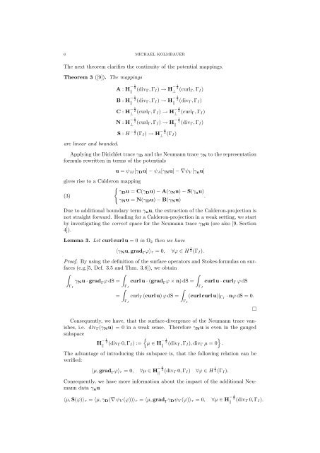
The next theorem clarifies the continuity of the potential mappings.
Theorem 3 ([9]). The mappings
are linear and bounded.
A : H − 1 2
‖
(div Γ , Γ I ) → H − 1 2
⊥ (curl Γ, Γ I )
B : H − 1 2
‖
(div Γ , Γ I ) → H − 1 2
‖
(div Γ , Γ I )
C : H − 1 2
⊥ (curl Γ, Γ I ) → H − 1 2
⊥ (curl Γ, Γ I )
N : H − 1 2
⊥ (curl Γ, Γ I ) → H − 1 2
‖
(div Γ , Γ I )
S : H − 1 2 (ΓI ) → H − 1 2
⊥ (Γ I)
Applying the Dirichlet trace γ D and the Neumann trace γ N to the representation
formula rewritten in terms of the potentials
gives rise to a Calderon mapping
u = ψ M [γ D u] − ψ A [γ N u] − ∇ψ V [γ n u]
(3)
{
γD u = C(γ D u) − A(γ N u) − S(γ n u)
.
γ N u = N(γ D u) − B(γ N u)
Due to additional boundary term γ n u, the extraction of the Calderon-projection is
not straight forward. Heading for a Calderon-projection in a weak setting, we start
by investigating the correct space for the Neumann trace γ N u (see also [9, Section
4]).
Lemma 3. Let curl curl u = 0 in Ω 2 then we have
〈γ N u, grad Γ ϕ〉 τ = 0, ∀ϕ ∈ H 1 2 (ΓI ).
Proof. By using the definition of the surface operators and Stokes-formulas on surfaces
(e.g.[5, Def. 3.5 and Thm. 3.8]), we obtain
∫
∫
∫
γ N u · grad Γ ϕ dS = curl u · (grad Γ ϕ × n) dS = curl u · curl Γ ϕ dS
Γ I Γ I Γ
∫
∫
I
= curl Γ (curl u) ϕ dS = (curl curl u)| ΓI · nϕ dS = 0.
Γ I Γ I
Consequently, we have, that the surface-divergence of the Neumann trace vanishes,
i.e. div Γ (γ N u) = 0 in a weak sense. Therefore γ N u is even in the gauged
subspace
{
}
H − 1 2
‖
(div Γ 0, Γ I ) := µ ∈ H − 1 2
‖
(div Γ , Γ I ), div Γ µ = 0 .
The advantage of introducing this subspace is, that the following relation can be
verified:
〈µ, grad Γ ϕ〉 τ = 0, ∀µ ∈ H − 1 2
‖
(div Γ 0, Γ I ) ∀ϕ ∈ H 1 2 (ΓI ).
Consequently, we have more information about the impact of the additional Neumann
data γ n u
〈µ, S(ϕ)〉 τ = 〈µ, γ D (∇ ψ V (ϕ))〉 τ = 〈µ, grad Γ γ D ψ V (ϕ)〉 τ = 0, ∀µ ∈ H − 1 2
‖
(div Γ 0, Γ I ).
□