Existence and Uniqueness of Eddy Current Problems in Bounded ...
Existence and Uniqueness of Eddy Current Problems in Bounded ...
Existence and Uniqueness of Eddy Current Problems in Bounded ...

Create successful ePaper yourself
Turn your PDF publications into a flip-book with our unique Google optimized e-Paper software.
JOHANNES KEPLER UNIVERSITY LINZ<br />
Institute <strong>of</strong> Computational Mathematics<br />
<strong>Existence</strong> <strong>and</strong> <strong>Uniqueness</strong> <strong>of</strong> <strong>Eddy</strong> <strong>Current</strong><br />
<strong>Problems</strong> <strong>in</strong> <strong>Bounded</strong> <strong>and</strong><br />
Unbounded Doma<strong>in</strong>s<br />
Michael Kolmbauer<br />
Institute <strong>of</strong> Computational Mathematics, Johannes Kepler University<br />
Altenberger Str. 69, 4040 L<strong>in</strong>z, Austria<br />
NuMa-Report No. 2011-03 May 2011<br />
A–4040 LINZ, Altenbergerstraße 69, Austria
Technical Reports before 1998:<br />
1995<br />
95-1 Hedwig Br<strong>and</strong>stetter<br />
Was ist neu <strong>in</strong> Fortran 90? March 1995<br />
95-2 G. Haase, B. Heise, M. Kuhn, U. Langer<br />
Adaptive Doma<strong>in</strong> Decomposition Methods for F<strong>in</strong>ite <strong>and</strong> Boundary Element August 1995<br />
Equations.<br />
95-3 Joachim Schöberl<br />
An Automatic Mesh Generator Us<strong>in</strong>g Geometric Rules for Two <strong>and</strong> Three Space August 1995<br />
Dimensions.<br />
1996<br />
96-1 Ferd<strong>in</strong><strong>and</strong> Kick<strong>in</strong>ger<br />
Automatic Mesh Generation for 3D Objects. February 1996<br />
96-2 Mario Goppold, Gundolf Haase, Bodo Heise und Michael Kuhn<br />
Preprocess<strong>in</strong>g <strong>in</strong> BE/FE Doma<strong>in</strong> Decomposition Methods. February 1996<br />
96-3 Bodo Heise<br />
A Mixed Variational Formulation for 3D Magnetostatics <strong>and</strong> its F<strong>in</strong>ite Element February 1996<br />
Discretisation.<br />
96-4 Bodo Heise und Michael Jung<br />
Robust Parallel Newton-Multilevel Methods. February 1996<br />
96-5 Ferd<strong>in</strong><strong>and</strong> Kick<strong>in</strong>ger<br />
Algebraic Multigrid for Discrete Elliptic Second Order <strong>Problems</strong>. February 1996<br />
96-6 Bodo Heise<br />
A Mixed Variational Formulation for 3D Magnetostatics <strong>and</strong> its F<strong>in</strong>ite Element<br />
Discretisation.<br />
May 1996<br />
96-7 Michael Kuhn<br />
Benchmark<strong>in</strong>g for Boundary Element Methods. June 1996<br />
1997<br />
97-1 Bodo Heise, Michael Kuhn <strong>and</strong> Ulrich Langer<br />
A Mixed Variational Formulation for 3D Magnetostatics <strong>in</strong> the Space H(rot)∩ February 1997<br />
H(div)<br />
97-2 Joachim Schöberl<br />
Robust Multigrid Precondition<strong>in</strong>g for Parameter Dependent <strong>Problems</strong> I: The June 1997<br />
Stokes-type Case.<br />
97-3 Ferd<strong>in</strong><strong>and</strong> Kick<strong>in</strong>ger, Sergei V. Nepomnyaschikh, Ralf Pfau, Joachim Schöberl<br />
Numerical Estimates <strong>of</strong> Inequalities <strong>in</strong> H 1 2 . August 1997<br />
97-4 Joachim Schöberl<br />
Programmbeschreibung NAOMI 2D und Algebraic Multigrid. September 1997<br />
From 1998 to 2008 technical reports were published by SFB013. Please see<br />
http://www.sfb013.uni-l<strong>in</strong>z.ac.at/<strong>in</strong>dex.php?id=reports<br />
From 2004 on reports were also published by RICAM. Please see<br />
http://www.ricam.oeaw.ac.at/publications/list/<br />
For a complete list <strong>of</strong> NuMa reports see<br />
http://www.numa.uni-l<strong>in</strong>z.ac.at/Publications/List/
EXISTENCE AND UNIQUENESS OF EDDY CURRENT<br />
PROBLEMS IN BOUNDED AND UNBOUNDED DOMAINS<br />
MICHAEL KOLMBAUER<br />
Abstract. This work is devoted to provid<strong>in</strong>g existence <strong>and</strong> uniqueness results<br />
for time-dependent eddy current problems <strong>in</strong> bounded <strong>and</strong> unbounded<br />
doma<strong>in</strong>s. There<strong>in</strong> we comb<strong>in</strong>e well known results for abstract evolution equations<br />
with boundary reduction methods like harmonic extensions <strong>and</strong> boundary<br />
<strong>in</strong>tegral operators.<br />
1. Introduction<br />
<strong>Eddy</strong> current problems are fundamental different for conduct<strong>in</strong>g <strong>and</strong> non-conduct<strong>in</strong>g<br />
regions. While <strong>in</strong> conduct<strong>in</strong>g regions the problems are <strong>of</strong> “parabolic“ type, <strong>in</strong><br />
non-conduct<strong>in</strong>g regions the problems reduce to ”elliptic” ones. In this work we<br />
want to analyze these PDEs <strong>of</strong> mixed type <strong>and</strong> provide existence <strong>and</strong> uniqueness<br />
results.<br />
In a conduct<strong>in</strong>g doma<strong>in</strong> Ω 1 ⊂ R 3 , the conductivity can be assumed to be piecewise<br />
constant <strong>and</strong> uniformly positive, i.e. σ ≥ σ 0 > 0 almost everywhere. Inside<br />
the conductor Ω 1 , the relation between the magnetic field H <strong>and</strong> the magnetic field<br />
density B can be <strong>in</strong> general nonl<strong>in</strong>ear. Neglect<strong>in</strong>g the effects <strong>of</strong> hysteresis, the relation<br />
is given by the B-H curve: H = ν 1 (B)B, where the reluctivity ν 1 is given by a<br />
cont<strong>in</strong>uous function ν 1 : R + 0 → R+ , satisfy<strong>in</strong>g the follow<strong>in</strong>g properties: s ↦→ ν 1 (s)s<br />
is strictly monotone <strong>and</strong> Lipschitz cont<strong>in</strong>uous <strong>and</strong> s ↦→ ν 1 (s) is uniformly positive<br />
<strong>and</strong> bounded. These properties are an immediate consequence <strong>of</strong> the physical<br />
background (see e.g. [10]). We mention, that the reluctivity satisfies the relation<br />
ν = µ −1 , where µ is the magnetic permeability. The excitation f 1 is provided by<br />
impressed currents or source currents. For simplicity we neglect permanent magnets.<br />
By <strong>in</strong>troduc<strong>in</strong>g a vector potential u for the magnetic field density B = curl u,<br />
the equation <strong>in</strong> the conduct<strong>in</strong>g doma<strong>in</strong> has the follow<strong>in</strong>g parabolic structure:<br />
σ(x) ∂u<br />
∂t + curl (ν 1(|curl u|) curl u) = f 1 .<br />
In a non-conduct<strong>in</strong>g doma<strong>in</strong> Ω 2 , the conductivity vanishes, i.e. σ = 0. Additionally<br />
the reluctivity ν 2 > 0 is constant <strong>and</strong> we assume that there is no source. Hence we<br />
deal with a stationary <strong>and</strong> elliptic curl-curl problem:<br />
curl (ν 2 curl u) = 0.<br />
A non-conduct<strong>in</strong>g doma<strong>in</strong> Ω 2 corresponds to the unbounded air region, <strong>and</strong> therefore<br />
is unbounded <strong>in</strong> general. Nevertheless we also analyze the case <strong>of</strong> a bounded air<br />
region, s<strong>in</strong>ce <strong>in</strong> many applications, the unbounded exterior doma<strong>in</strong> is approximated<br />
by a bounded one with homogeneous boundary conditions imposed some distance<br />
away from the conductor.<br />
In order to provide existence <strong>and</strong> uniqueness results for a general eddy current<br />
problem consist<strong>in</strong>g <strong>of</strong> both conduct<strong>in</strong>g <strong>and</strong> non-conduct<strong>in</strong>g doma<strong>in</strong>s, the ma<strong>in</strong> tool<br />
is the reduction <strong>of</strong> the full computational doma<strong>in</strong> to the conduct<strong>in</strong>g doma<strong>in</strong> only.<br />
The authors gratefully acknowledge the f<strong>in</strong>ancial support by the Austrian Science Fund (FWF)<br />
under the grant P19255 <strong>and</strong> DK W1214.<br />
1
2 MICHAEL KOLMBAUER<br />
This can be achieved by either us<strong>in</strong>g the framework <strong>of</strong> pde-harmonic extensions or<br />
by the framework <strong>of</strong> boundary <strong>in</strong>tegral operators.<br />
<strong>Eddy</strong> current problems <strong>in</strong> bounded doma<strong>in</strong>s have already been analyzed <strong>in</strong> [3, 4].<br />
They used pde-harmonic extensions to reduce the full computational doma<strong>in</strong> to the<br />
conduct<strong>in</strong>g doma<strong>in</strong>s only <strong>and</strong> provided existence <strong>and</strong> uniqueness results <strong>in</strong> special<br />
gauged spaces. Nevertheless we want to clarify their prov<strong>in</strong>g techniques <strong>and</strong> the<br />
computational details. For other works us<strong>in</strong>g similar techniques we mention [2].<br />
In order to extend the existence <strong>and</strong> uniqueness theory also to the case <strong>of</strong> unbounded<br />
doma<strong>in</strong>s, <strong>in</strong> pr<strong>in</strong>ciple the same approach <strong>of</strong> pde-harmonic extensions can<br />
be used. The drawback <strong>of</strong> the latter mentioned approach is the need for <strong>in</strong>troduc<strong>in</strong>g<br />
weighted Sobolev spaces, s<strong>in</strong>ce we are deal<strong>in</strong>g with an unbounded doma<strong>in</strong>. In<br />
order to avoid this, we prefer to use the theoretical framework <strong>of</strong> boundary <strong>in</strong>tegral<br />
operators. Additionally this approach directly <strong>of</strong>fers a start<strong>in</strong>g po<strong>in</strong>t for a doma<strong>in</strong><br />
decomposition method <strong>in</strong> the terms <strong>of</strong> a FEM-BEM (F<strong>in</strong>ite Element-Boundary<br />
Element) coupl<strong>in</strong>g.<br />
Indeed the symmetric coupl<strong>in</strong>g <strong>of</strong> eddy current problems <strong>in</strong> the frequency doma<strong>in</strong><br />
is well understood [9]. In contrast to the latter mentioned approach, we do not<br />
switch from the time doma<strong>in</strong> to the frequency doma<strong>in</strong>, <strong>and</strong> hence we have to deal<br />
with a time-dependent problem. Nevertheless we can comb<strong>in</strong>e well known existence<br />
<strong>and</strong> uniqueness results for parabolic problems [12, 13] <strong>and</strong> the technique <strong>of</strong> symmetric<br />
coupl<strong>in</strong>g [8] to obta<strong>in</strong> existence <strong>and</strong> uniqueness also <strong>in</strong> the time doma<strong>in</strong>. For<br />
another approach us<strong>in</strong>g these techniques for time-dependent eddy current problems<br />
we mention [1].<br />
The rest <strong>of</strong> the paper is organized as follows: In Section 2 we provide st<strong>and</strong>ard<br />
existence <strong>and</strong> uniqueness results for abstract evolution equations. After that,<br />
the basic function spaces <strong>and</strong> traces for Maxwell’s equations are <strong>in</strong>troduced. Furthermore<br />
we collect some useful results for eddy current problems <strong>in</strong> conduct<strong>in</strong>g<br />
doma<strong>in</strong>s. In Section 3 <strong>and</strong> 4 the ma<strong>in</strong> results, the existence <strong>and</strong> uniqueness <strong>of</strong> eddy<br />
current problems are presented for the case <strong>of</strong> unbounded <strong>and</strong> bounded doma<strong>in</strong>s,<br />
respectively.<br />
2. Some prelim<strong>in</strong>ary results<br />
2.1. <strong>Existence</strong> <strong>and</strong> uniqueness <strong>of</strong> abstract evolution equations. The basis<br />
for prov<strong>in</strong>g existence <strong>and</strong> uniqueness <strong>of</strong> degenerated parabolic problems, is the<br />
abstract theory for abstract evolution equations. For details we refer to [12] <strong>and</strong><br />
[13] for l<strong>in</strong>ear <strong>and</strong> nonl<strong>in</strong>ear equations, respectively. We just quote the result<strong>in</strong>g<br />
theorems for operator equations <strong>of</strong> parabolic type.<br />
Theorem 1 (Nonl<strong>in</strong>ear). Let V ⊂ H ⊂ V ∗ be an evolution triple. Let A : V → V ∗<br />
be a hemicont<strong>in</strong>uous, monotone, coercive <strong>and</strong> bounded operator. Suppose furthermore<br />
that F ∈ L 2 ((0, T ), V ∗ ) <strong>and</strong> u 0 ∈ H be given. Then the <strong>in</strong>itial value problem<br />
d<br />
dt u(t) + A(u(t)) = F (t), <strong>in</strong> L 2(0, T ; V ∗ )<br />
u(0) = u 0 , <strong>in</strong> H<br />
has a unique solution u ∈ L 2 ((0, T ), V ) with weak derivative ˙u ∈ L 2 ((0, T ), V ∗ ).<br />
Pro<strong>of</strong>. [13, Theorem 30.A], see also [13, Corollary 30.12]<br />
Theorem 2 (L<strong>in</strong>ear). Let V ⊂ H ⊂ V ∗ be an evolution triple. Let A : V → V ∗ be<br />
a l<strong>in</strong>ear, coercive <strong>and</strong> bounded operator. Suppose furthermore that F ∈ L 2 (0, T ; V ∗ )<br />
<strong>and</strong> u 0 ∈ H be given. Then the <strong>in</strong>itial value problem<br />
d<br />
dt u(t) + Au(t) = F (t), <strong>in</strong> L 2(0, T ; V ∗ )<br />
u(0) = u 0 , <strong>in</strong> H<br />
has a unique solution u ∈ L 2 ((0, T ), V ) with weak derivative ˙u ∈ L 2 ((0, T ), V ∗ ).<br />
□
Pro<strong>of</strong>. [12, Theorem 23.A]<br />
EXISTENCE AND UNIQUENESS 3<br />
2.2. Spaces <strong>and</strong> trace spaces for Maxwell’s equations. In this Section we<br />
briefly summarize the underly<strong>in</strong>g space <strong>and</strong> the correct trace spaces for the eddy<br />
current problem. Therefore, <strong>in</strong> this Section let Ω ⊂ R 3 be a simply connected<br />
polyhedron with boundary Γ. The underly<strong>in</strong>g Hilbert space is<br />
H(curl, Ω) := {u ∈ L 2 (Ω) : curl u ∈ L 2 (Ω)}.<br />
For the traces we fix the follow<strong>in</strong>g notations<br />
γ D u := n×(u| Γ ×n) γ × u := u| Γ ×n γ N u := curl u| Γ ×n γ n u := n·u| Γ ,<br />
where n denotes the exterior normal <strong>of</strong> Ω on the boundary Γ. For the def<strong>in</strong>ition <strong>of</strong><br />
the appropriate trace spaces, please recall the def<strong>in</strong>itions <strong>of</strong> the surface differential<br />
operators grad Γ , curl Γ , curl Γ , div Γ (see e.g. [6, 7]). The appropriate trace spaces<br />
for polyhedral doma<strong>in</strong>s have been <strong>in</strong>troduced by Buffa <strong>and</strong> Ciarlet <strong>in</strong> [6, 7]. The<br />
space for the Dirichlet trace γ D <strong>and</strong> the Neumann trace γ N are given by<br />
H − 1 2<br />
⊥ (curl Γ, Γ) := {v ∈ H − 1 2<br />
⊥<br />
(Γ), curl Γv ∈ H − 1 2 (Γ)}<br />
H − 1 2<br />
‖<br />
(div Γ , Γ) := {v ∈ H − 1 2<br />
‖<br />
(Γ), div Γ v ∈ H − 1 2 (Γ)}.<br />
Indeed H − 1 2<br />
⊥ (curl Γ, Γ) is the dual <strong>of</strong> H − 1 2<br />
‖<br />
(div Γ , Γ) <strong>and</strong> vice versa. The correspond<strong>in</strong>g<br />
duality product is the extension <strong>of</strong> the L 2 t (Γ) duality product <strong>and</strong> <strong>in</strong> the follow<strong>in</strong>g<br />
will be denoted with subscript τ:<br />
〈·, ·〉 τ<br />
:= 〈·, ·〉<br />
H<br />
− 1 2<br />
‖ (div Γ,Γ)×H − 1 2<br />
⊥ (curlΓ,Γ) .<br />
For u ∈ H(curl curl, R 3 \Ω) := {u ∈ H(curl, R 3 \Ω) : curl curl u ∈ L 2 (R 3 \Ω)}<br />
the <strong>in</strong>tegration by parts formula for the exterior doma<strong>in</strong> R 3 \Ω holds<br />
〈γ N u, γ D v〉 τ = −(curl u, curl v) L2(R 3 \Ω) + (curl curl u, v) L2(R 3 \Ω).<br />
The Dirichlet <strong>and</strong> Neumann trace can be extended to cont<strong>in</strong>uous mapp<strong>in</strong>gs.<br />
Lemma 1 ([6, 7, 9]). The trace operators<br />
are l<strong>in</strong>ear, cont<strong>in</strong>uous <strong>and</strong> surjective.<br />
γ D : H(curl, Ω) → H − 1 2<br />
⊥ (curl Γ, Γ)<br />
γ × : H(curl, Ω) → H − 1 2<br />
‖<br />
(div Γ , Γ)<br />
γ N : H(curl curl, Ω) → H − 1 2<br />
‖<br />
(div Γ , Γ)<br />
2.3. <strong>Eddy</strong> current problems <strong>in</strong> conduct<strong>in</strong>g doma<strong>in</strong>s. In this Section we collect<br />
some useful auxiliary results from the analysis <strong>of</strong> the eddy current problem <strong>in</strong><br />
conduct<strong>in</strong>g regions. In this case the existence <strong>and</strong> uniqueness is well understood<br />
(see e.g. [3, 4]). Indeed the difficulty <strong>of</strong> deal<strong>in</strong>g with the nonl<strong>in</strong>earity, result<strong>in</strong>g<br />
from the nonl<strong>in</strong>earity <strong>of</strong> the B-H curve, are discussed. Let the nonl<strong>in</strong>ear operator<br />
A be def<strong>in</strong>ed by<br />
∫<br />
〈A(u), v〉 := ν 1 (|curl u|)curl u · curl v dx,<br />
Ω 1<br />
where 〈·, ·〉 denotes the duality product. The ma<strong>in</strong> properties <strong>of</strong> A are summarized<br />
<strong>in</strong> the follow<strong>in</strong>g lemma.<br />
Lemma 2. Let s ↦→ ν 1 (s)s be strictly monotone <strong>and</strong> Lipschitz cont<strong>in</strong>uous <strong>and</strong><br />
s ↦→ ν 1 (s) uniformly positive <strong>and</strong> bounded, then the operator A is<br />
• monotone, i.e. 〈A(u) − A(v), u − v〉 ≥ 0<br />
□
4 MICHAEL KOLMBAUER<br />
I n<br />
n 2<br />
n 1<br />
2<br />
Σ⩵0<br />
air<br />
1<br />
Σ0<br />
conductor<br />
Figure 1. Unbounded exterior doma<strong>in</strong><br />
• semi-coercive, i.e. 〈A(u), u〉 ≥ c‖ curl u‖ 2 L 2(Ω)<br />
• bounded, i.e. 〈A(u), v〉 ≤ c‖u‖ H(curl,Ω) ‖v‖ H(curl,Ω)<br />
• hemicont<strong>in</strong>uous.<br />
Pro<strong>of</strong>. see [3, Lemma 2.6].<br />
For l<strong>in</strong>ear operators the whole analysis simplifies as the follow<strong>in</strong>g remark states.<br />
Remark 1. Let M be any l<strong>in</strong>ear operator. If M is semi-coercive, i.e. 〈M(w), w〉 ≥<br />
0, then M is also monotone.<br />
Hence the operator A result<strong>in</strong>g from the conduct<strong>in</strong>g part <strong>of</strong> our computational<br />
doma<strong>in</strong> naturally fulfills the requirements <strong>of</strong> Theorem 1 <strong>and</strong> Theorem 2. Therefore<br />
the idea <strong>of</strong> reduc<strong>in</strong>g the computational doma<strong>in</strong> to the conduct<strong>in</strong>g parts only, arises<br />
quite natural <strong>in</strong> this context.<br />
3. The eddy current problem <strong>in</strong> R 3<br />
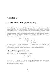
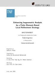
Let Ω be R 3 <strong>and</strong> consist <strong>of</strong> two subdoma<strong>in</strong>s, Ω 1 <strong>and</strong> Ω 2 , with the follow<strong>in</strong>g properties.<br />
Ω 1 is Lipschitz polyhedron that is simply connected. Ω 2 is the complement<br />
<strong>of</strong> Ω 1 <strong>in</strong> R 3 , i.e R 3 \Ω 1 , <strong>and</strong> hence also simply connected. Furthermore we denote<br />
by Γ I the <strong>in</strong>terface <strong>of</strong> the two subdoma<strong>in</strong>s, i.e. Γ I = Ω 1 ∩ Ω 2 . By n we denote the<br />
exterior unit normal vector field <strong>of</strong> Ω 1 on Γ I , po<strong>in</strong>t<strong>in</strong>g from Ω 1 to Ω 2 (see Figure 1).<br />
Additionally to the partial differential equations <strong>in</strong> Ω 1 <strong>and</strong> Ω 2 , the solution has to<br />
be s<strong>in</strong>usoidal <strong>in</strong> Ω 2 . The system is completed by appropriate decay <strong>and</strong> <strong>in</strong>terface<br />
conditions <strong>and</strong> an <strong>in</strong>itial condition. Hence we deal with the follow<strong>in</strong>g problem:<br />
(1)<br />
⎧<br />
⎪⎨<br />
⎪⎩<br />
∂u<br />
σ 1 ∂t + curl (ν 1(|curl u|) curl u) = f 1 , <strong>in</strong> Ω 1 × (0, T )<br />
curl (curl u) = 0 <strong>in</strong> Ω 2 × (0, T )<br />
div u = 0 <strong>in</strong> Ω 2 × (0, T )<br />
u = O(|x| −1 ) for |x| → ∞<br />
curl u = O(|x| −1 ) for |x| → ∞<br />
u = u 0 on Ω 1 × {0}<br />
u 1 × n = u 2 × n on Γ I × (0, T )<br />
ν 1 (|curl u 1 |)curl u 1 × n = curl u 2 × n on Γ I × (0, T )<br />
Here u 1 <strong>and</strong> u 2 are the restrictions <strong>of</strong> u to Ω 1 <strong>and</strong> Ω 2 , i.e. u 1 = u| Ω1 <strong>and</strong> u 2 = u| Ω2 .<br />
Remark 2. Due to scal<strong>in</strong>g arguments, it can always be achieved that ν 2 = 1.<br />
(Otherwise ν 1 = ν 1 /ν 2 <strong>and</strong> σ 1 = σ 1 /ν 1 .)<br />
We show, that the degenerated parabolic problem on the whole doma<strong>in</strong> (1) can<br />
be reduced to an <strong>in</strong>itial value problem <strong>in</strong> the conduct<strong>in</strong>g region by us<strong>in</strong>g the tools<br />
<strong>of</strong> boundary <strong>in</strong>tegral operators. For the result<strong>in</strong>g parabolic equation, st<strong>and</strong>ard<br />
□
EXISTENCE AND UNIQUENESS 5<br />
arguments provide existence <strong>and</strong> uniqueness. The crucial po<strong>in</strong>t <strong>in</strong> the pro<strong>of</strong> is to<br />
verify the coercivity <strong>of</strong> the result<strong>in</strong>g l<strong>in</strong>ear or nonl<strong>in</strong>ear operator <strong>and</strong> this is done<br />
<strong>in</strong> detail. The start<strong>in</strong>g po<strong>in</strong>t <strong>of</strong> our analysis is the l<strong>in</strong>e-variational formulation.<br />
By Multiply<strong>in</strong>g by a test function only depend<strong>in</strong>g on the space variable x <strong>and</strong><br />
<strong>in</strong>tegrat<strong>in</strong>g over the computational doma<strong>in</strong> Ω, we arrive at the follow<strong>in</strong>g variational<br />
form.<br />
[<br />
] ∫<br />
∫<br />
∂u<br />
σ 1<br />
∫Ω 1<br />
∂t v + ν 1(|curl u|)curl u · curl v dx+ ν 2 curl u·curl v dx = f 1·v dx<br />
Ω 2 Ω 1<br />
Apply<strong>in</strong>g <strong>in</strong>tegration by parts <strong>in</strong> the exterior doma<strong>in</strong> Ω 2 once more <strong>and</strong> us<strong>in</strong>g the<br />
fact, that there is no prescribed source <strong>in</strong> Ω 2 , i.e. curl curl u = 0, allows to reduce<br />
the variational problem to one just liv<strong>in</strong>g <strong>in</strong> Ω 1 .<br />
∫Ω 1<br />
[<br />
σ 1<br />
∂u<br />
∂t v + ν 1(|curl u|)curl u · curl v<br />
] ∫<br />
dx −<br />
γ N u · γ D v dS =<br />
Γ<br />
}<br />
I<br />
{{ }<br />
=〈γ N u,γ D v〉 τ<br />
∫<br />
Ω 1<br />
f 1 · v dx<br />
In order to analyze this variational form we fix the time t. The first step is the<br />
<strong>in</strong>troduction <strong>of</strong> the framework <strong>of</strong> boundary <strong>in</strong>tegral equations for the part correspond<strong>in</strong>g<br />
to the <strong>in</strong>terface Γ I . Therefore we strongly follow the approach <strong>of</strong> Hiptmair<br />
for the frequency doma<strong>in</strong> approach [9]. The boundary <strong>in</strong>tegral equations for the<br />
exterior problem emerge from a representation formula. In the case <strong>of</strong> Maxwell’s<br />
equation this is the Stratton-Chu formula, that <strong>in</strong>volves the fundamental solution<br />
<strong>of</strong> the Laplacian <strong>in</strong> three dimensions.<br />
∫<br />
u(x) = (n × curl u)(y)E(x, y) dS y − curl x (n × u)(y)E(x, y) dS y<br />
∫Γ I Γ<br />
∫<br />
I<br />
(2) + ∇ x (n · u)(y)E(x, y) dS y + curl curl u(y)E(x, y) dy<br />
∫Γ I Ω<br />
∫<br />
2<br />
− div u(y)∇ x E(x, y) dy.<br />
Ω 2<br />
The fundamental solution <strong>of</strong> the Laplacian <strong>in</strong> three dimensions is given by<br />
E(x, y) := 1 1<br />
4π |x − y| , x, y ∈ R3 , x ≠ y.<br />
Note, that due to curl curl u = 0 <strong>and</strong> div u = 0, the last two terms <strong>in</strong> (2) vanish.<br />
Next we <strong>in</strong>troduce the vectorial s<strong>in</strong>gle layer potential ψ A , the vectorial double layer<br />
potentials ψ M <strong>and</strong> the scalar s<strong>in</strong>gle layer potential ψ V :<br />
∫<br />
ψ A (u)(x) := u(y)E(x, y) dS y<br />
Γ I<br />
ψ M (n × u)(x) := curl x (n × u)(y)E(x, y) dS y<br />
∫Γ<br />
∫<br />
I<br />
ψ V (n · u)(x) := (n · u)(y)E(x, y) dS y<br />
Γ I<br />
Tak<strong>in</strong>g the Dirichlet <strong>and</strong> Neumann traces <strong>of</strong> these potential operators gives rise to<br />
the def<strong>in</strong>ition <strong>of</strong> the boundary <strong>in</strong>tegral operators.<br />
Aλ := γ D ψ A (λ)<br />
Bλ := γ N ψ A (λ)<br />
Cu := γ D ψ M (u)<br />
Nu := γ N ψ M (u)<br />
Sϕ := γ D (∇ ψ V (ϕ)).
6 MICHAEL KOLMBAUER<br />
The next theorem clarifies the cont<strong>in</strong>uity <strong>of</strong> the potential mapp<strong>in</strong>gs.<br />
Theorem 3 ([9]). The mapp<strong>in</strong>gs<br />
are l<strong>in</strong>ear <strong>and</strong> bounded.<br />
A : H − 1 2<br />
‖<br />
(div Γ , Γ I ) → H − 1 2<br />
⊥ (curl Γ, Γ I )<br />
B : H − 1 2<br />
‖<br />
(div Γ , Γ I ) → H − 1 2<br />
‖<br />
(div Γ , Γ I )<br />
C : H − 1 2<br />
⊥ (curl Γ, Γ I ) → H − 1 2<br />
⊥ (curl Γ, Γ I )<br />
N : H − 1 2<br />
⊥ (curl Γ, Γ I ) → H − 1 2<br />
‖<br />
(div Γ , Γ I )<br />
S : H − 1 2 (ΓI ) → H − 1 2<br />
⊥ (Γ I)<br />
Apply<strong>in</strong>g the Dirichlet trace γ D <strong>and</strong> the Neumann trace γ N to the representation<br />
formula rewritten <strong>in</strong> terms <strong>of</strong> the potentials<br />
gives rise to a Calderon mapp<strong>in</strong>g<br />
u = ψ M [γ D u] − ψ A [γ N u] − ∇ψ V [γ n u]<br />
(3)<br />
{<br />
γD u = C(γ D u) − A(γ N u) − S(γ n u)<br />
.<br />
γ N u = N(γ D u) − B(γ N u)<br />
Due to additional boundary term γ n u, the extraction <strong>of</strong> the Calderon-projection is<br />
not straight forward. Head<strong>in</strong>g for a Calderon-projection <strong>in</strong> a weak sett<strong>in</strong>g, we start<br />
by <strong>in</strong>vestigat<strong>in</strong>g the correct space for the Neumann trace γ N u (see also [9, Section<br />
4]).<br />
Lemma 3. Let curl curl u = 0 <strong>in</strong> Ω 2 then we have<br />
〈γ N u, grad Γ ϕ〉 τ = 0, ∀ϕ ∈ H 1 2 (ΓI ).<br />
Pro<strong>of</strong>. By us<strong>in</strong>g the def<strong>in</strong>ition <strong>of</strong> the surface operators <strong>and</strong> Stokes-formulas on surfaces<br />
(e.g.[5, Def. 3.5 <strong>and</strong> Thm. 3.8]), we obta<strong>in</strong><br />
∫<br />
∫<br />
∫<br />
γ N u · grad Γ ϕ dS = curl u · (grad Γ ϕ × n) dS = curl u · curl Γ ϕ dS<br />
Γ I Γ I Γ<br />
∫<br />
∫<br />
I<br />
= curl Γ (curl u) ϕ dS = (curl curl u)| ΓI · nϕ dS = 0.<br />
Γ I Γ I<br />
Consequently, we have, that the surface-divergence <strong>of</strong> the Neumann trace vanishes,<br />
i.e. div Γ (γ N u) = 0 <strong>in</strong> a weak sense. Therefore γ N u is even <strong>in</strong> the gauged<br />
subspace<br />
{<br />
}<br />
H − 1 2<br />
‖<br />
(div Γ 0, Γ I ) := µ ∈ H − 1 2<br />
‖<br />
(div Γ , Γ I ), div Γ µ = 0 .<br />
The advantage <strong>of</strong> <strong>in</strong>troduc<strong>in</strong>g this subspace is, that the follow<strong>in</strong>g relation can be<br />
verified:<br />
〈µ, grad Γ ϕ〉 τ = 0, ∀µ ∈ H − 1 2<br />
‖<br />
(div Γ 0, Γ I ) ∀ϕ ∈ H 1 2 (ΓI ).<br />
Consequently, we have more <strong>in</strong>formation about the impact <strong>of</strong> the additional Neumann<br />
data γ n u<br />
〈µ, S(ϕ)〉 τ = 〈µ, γ D (∇ ψ V (ϕ))〉 τ = 〈µ, grad Γ γ D ψ V (ϕ)〉 τ = 0, ∀µ ∈ H − 1 2<br />
‖<br />
(div Γ 0, Γ I ).<br />
□
EXISTENCE AND UNIQUENESS 7<br />
Us<strong>in</strong>g the last identity, we can set the Calderon mapp<strong>in</strong>g <strong>in</strong> a weak sett<strong>in</strong>g. Test<strong>in</strong>g<br />
with appropriate test functions µ <strong>and</strong> λ yields<br />
⎧<br />
⎨ 〈µ, γ D u〉 τ<br />
= 〈µ, C(γ D u)〉 τ<br />
− 〈µ, A(γ N u)〉 τ<br />
, ∀µ ∈ H − 1 2<br />
‖<br />
(div Γ 0, Γ I )<br />
(4)<br />
⎩<br />
〈γ N u, λ〉 τ<br />
= 〈N(γ D u), λ〉 τ<br />
− 〈B(γ N u), λ〉 τ<br />
, ∀λ ∈ H − 1 2<br />
⊥ (curl Γ, Γ I ).<br />
In the follow<strong>in</strong>g Lemmata we collect several properties <strong>of</strong> the boundary <strong>in</strong>tegral<br />
operators A, B, C <strong>and</strong> N.<br />
Lemma 4. The bil<strong>in</strong>ear form on H − 1 2<br />
‖<br />
(div Γ 0, Γ I ) <strong>in</strong>duced by the operator A is<br />
symmetric <strong>and</strong> positive def<strong>in</strong>ite.<br />
Pro<strong>of</strong>. see [9, Thm 6.2]<br />
〈λ, Aλ〉 τ ≥ c A 1 ‖λ‖ 2 , ∀λ ∈ H − 1<br />
H − 2<br />
1 2<br />
‖<br />
(div Γ 0, Γ).<br />
(div ‖ Γ,Γ)<br />
Lemma 5. We have the symmetry property<br />
〈B(µ), λ〉 τ = 〈µ, (C − Id)(λ)〉 τ , ∀µ ∈ H − 1 2<br />
‖<br />
(div Γ 0, Γ), λ ∈ H − 1 2<br />
⊥<br />
(curl Γ, Γ).<br />
Pro<strong>of</strong>. see [9, Eqn. (6.5)].<br />
□<br />
□<br />
Lemma 6. The bil<strong>in</strong>ear form on H − 1 2<br />
⊥<br />
(curl Γ, Γ I ) <strong>in</strong>duced by the operator N is<br />
symmetric <strong>and</strong> negative semi-def<strong>in</strong>ite.<br />
Pro<strong>of</strong>. see [9, Thm 6.4]<br />
−〈Nµ, µ〉 τ ≥ c‖curl Γ µ‖ 2 H − 1 2 (Γ) , ∀µ ∈ H− 1 2<br />
⊥ (curl Γ, Γ)<br />
The follow<strong>in</strong>g Lemma plays an important role for provid<strong>in</strong>g the coercivity result,<br />
needed for prov<strong>in</strong>g existence <strong>and</strong> uniqueness.<br />
Lemma 7. We have<br />
−〈γ N u, γ D u〉 τ ≥ 0.<br />
Pro<strong>of</strong>. Us<strong>in</strong>g the weak Calderon mapp<strong>in</strong>g (4) <strong>and</strong> choos<strong>in</strong>g special test functions<br />
µ = γ N u <strong>and</strong> λ = γ D u we obta<strong>in</strong> from the first equation <strong>and</strong> the symmetry property<br />
(Lemma 5)<br />
〈γ N u, A(γ N u)〉 τ<br />
= 〈γ N u, (C − Id)(γ D u)〉 τ<br />
= 〈B(γ N u), γ D u〉 τ<br />
.<br />
Consequently from the second equation we obta<strong>in</strong><br />
− 〈γ N u, γ D u〉 τ<br />
= − 〈N(γ D u), γ D u〉 τ<br />
+ 〈B(γ N u), γ D u〉 τ<br />
= − 〈N(γ D u), γ D u〉 τ<br />
+ 〈γ N u, A(γ N u)〉 τ<br />
.<br />
Now the result follows from the negative semi-def<strong>in</strong>iteness <strong>of</strong> N <strong>and</strong> the positive<br />
def<strong>in</strong>iteness <strong>of</strong> A.<br />
□<br />
Now we have provided the necessary tools for prov<strong>in</strong>g existence <strong>and</strong> uniqueness<br />
for the variational problem: F<strong>in</strong>d u ∈ L 2 ((0, T ), H(curl, Ω)) with a weak derivative<br />
˙u ∈ L 2 ((0, T ), H(curl, Ω) ∗ ), such that<br />
〈σ 1<br />
∂u<br />
∂t , v〉 + 〈A(u), v〉 − 〈γ Nu, γ D v〉 τ = 〈F, v〉<br />
for all v ∈ H(curl, Ω). As outl<strong>in</strong>ed <strong>in</strong> Section 2.3, we have that A is positive semidef<strong>in</strong>ite.<br />
Due to the positivity <strong>of</strong> the boundary term (Lemma 7), we can conclude<br />
that<br />
〈A(u), u〉 − 〈γ N u, γ D u〉 τ ≥ c‖ curl u‖ 2 L 2(Ω 1) .<br />
□
8 MICHAEL KOLMBAUER<br />
Indeed this estimate is too weak to obta<strong>in</strong> coercivity <strong>in</strong> the full space H(curl, Ω 1 ).<br />
Even the boundary term does not fix this problem s<strong>in</strong>ce the whole expression vanishes<br />
for v ∈ W(Ω 1 ). Here W(Ω 1 ) denotes the space <strong>of</strong> gradients, given by<br />
W(Ω 1 ) := {w = ∇ϕ : ϕ ∈ H 1 (Ω 1 ) <strong>and</strong> ϕ = c on Γ}.<br />
In order to be able to prove coercivity <strong>in</strong> the full norm, we have to restrict H(curl, Ω 1 )<br />
to the space <strong>of</strong> weakly divergence free functions. Consequently we <strong>in</strong>troduce the<br />
gauged subspace ¯V given by<br />
(5) ¯V := {u 1 ∈ H(curl, Ω 1 ) : (u 1 , w 1 ) L2(Ω 1) = 0, ∀ w 1 ∈ W(Ω 1 )}<br />
In the gauged subspace ¯V the full norm ‖·‖ H(curl,Ω) is equivalent to the semi-norm<br />
‖ curl ·‖ L2(Ω), as the follow<strong>in</strong>g Lemma states.<br />
Lemma 8 (Friedrich’s <strong>in</strong>equality). Let Ω 1 be a simply-connected Lipschitz doma<strong>in</strong>.<br />
For all u ∈ ¯V we have<br />
Pro<strong>of</strong>. see [11, Thm 3.26]<br />
‖u‖ L2(Ω 1) ≤ c‖ curl u‖ L2(Ω 1).<br />
Therefore the variational formulation restricted to this gauged subspace reads<br />
as: F<strong>in</strong>d u ∈ L 2 ((0, T ), ¯V), with a weak derivative ˙u ∈ L 2 ((0, T ), ¯V ∗ ), such that<br />
(6) 〈σ 1<br />
∂u<br />
∂t , v〉 + 〈A(u), v〉 − 〈γ Nu, γ D v〉 τ = 〈F, v〉<br />
for all v ∈ ¯V. Analogous, by def<strong>in</strong><strong>in</strong>g<br />
〈Mu, v〉 := 〈γ N u, γ D v〉 τ<br />
the correspond<strong>in</strong>g operator equation is given by: F<strong>in</strong>d u ∈ L 2 ((0, T ), ¯V) with a<br />
weak derivative ˙u ∈ L 2 ((0, T ), ¯V ∗ ), such that<br />
A(u) − Mu = F, <strong>in</strong> L 2 ((0, T ), ¯V ∗ )<br />
u(0) = u 0 , <strong>in</strong> L 2 (Ω 1 )<br />
Due to Lemma 8, we obta<strong>in</strong> coercivity <strong>in</strong> ¯V. S<strong>in</strong>ce the operator associated to<br />
the boundary part M is l<strong>in</strong>ear, hemicont<strong>in</strong>uity <strong>and</strong> monotonicity follow due to<br />
Lemma 2. <strong>Bounded</strong>ness <strong>of</strong> M follows by apply<strong>in</strong>g the trace theorems (Lemma 1.<br />
Note that curl curl u = 0 <strong>in</strong> the exterior doma<strong>in</strong>.) The precedent considerations<br />
<strong>in</strong> comb<strong>in</strong>ation with Theorem 1 give rise to the ma<strong>in</strong> result <strong>of</strong> this Section:<br />
Theorem 4. The variational problem (6) has a unique solution u ∈ L 2 ((0, T ), ¯V)<br />
with ˙u ∈ L 2 ((0, T ), ¯V ∗ ).<br />
In the next step we show, that under additional assumptions, we even can guarantee<br />
uniqueness <strong>in</strong> the non-gauged space L 2 ((0, T ), H(curl, Ω 1 )). We consider a<br />
test function w ∈ W(Ω 1 ).<br />
∫<br />
∫<br />
∫<br />
∫<br />
∂u<br />
σ 1<br />
Ω 1<br />
∂t w dx + ν 1 curl u · curl w dx − γ N u · γ D w dS = f 1 · w dx<br />
Ω 1 Γ I Ω 1<br />
Now we assume that the source f 1 <strong>and</strong> the <strong>in</strong>itial condition u 0 are weakly divergence<br />
free, i.e.<br />
(7)<br />
∫<br />
f 1 · w dx = 0<br />
Ω 1<br />
<strong>and</strong><br />
∫<br />
u 0 · w dx = 0,<br />
Ω 1<br />
∀w ∈ W(Ω 1 ).<br />
In order to show that u(t) is weakly divergence free for all time t we apply Lemma 3<br />
<strong>and</strong> recall the def<strong>in</strong>ition <strong>of</strong> the surface gradient grad Γ (p| Γ ) = γ D (∇p), ∀p ∈ H 1 (Ω 1 ).<br />
So, comb<strong>in</strong><strong>in</strong>g these two results, for constant σ 1 we arrive at<br />
∫<br />
∂u<br />
σ 1<br />
∂t w dx = 0, ∀w ∈ W(Ω 1).<br />
Ω 1<br />
□
EXISTENCE AND UNIQUENESS 9<br />
<br />
n<br />
n 2<br />
I n<br />
2<br />
Σ⩵0<br />
air<br />
1<br />
Σ0<br />
conductor<br />
n 2<br />
n 1<br />
Figure 2. <strong>Bounded</strong> doma<strong>in</strong>s<br />
S<strong>in</strong>ce the <strong>in</strong>itial condition u 0 is weakly divergence free, we can conclude that u(t)<br />
is weakly divergence-free for all t. Consequently for fixed t the solution u(t) is an<br />
element <strong>of</strong> the gauged space ¯V, a subspace <strong>of</strong> H(curl, Ω 1 ), where we have already<br />
proven existence <strong>and</strong> uniqueness. Summariz<strong>in</strong>g, if we claim the given data (f 1 <strong>and</strong><br />
u 0 ) to be s<strong>in</strong>usoidal, then neither the ¯V gaug<strong>in</strong>g <strong>in</strong> the conduct<strong>in</strong>g doma<strong>in</strong> Ω 1 nor<br />
the H − 1 2<br />
‖<br />
(div Γ 0, Γ) gaug<strong>in</strong>g on the <strong>in</strong>terface Γ I has to be enforced explicitly, s<strong>in</strong>ce<br />
they are fulfilled <strong>in</strong> a natural way.<br />
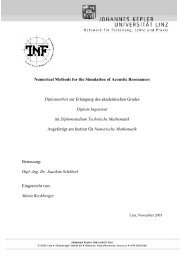
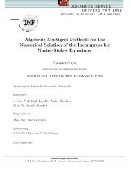
4. The eddy current problem <strong>in</strong> a bounded doma<strong>in</strong><br />
In this Section the unbounded exterior doma<strong>in</strong> Ω 2 is approximated by a bounded<br />
doma<strong>in</strong> by <strong>in</strong>troduc<strong>in</strong>g some artificial boundary some distance away from the conductor.<br />
Therefore let Ω ⊂ R 3 be a bounded Lipschitz doma<strong>in</strong>, consist<strong>in</strong>g <strong>of</strong> two<br />
subdoma<strong>in</strong>s Ω 1 <strong>and</strong> Ω 2 , i.e. ¯Ω = ¯Ω 1 ∩ ¯Ω 2 . Aga<strong>in</strong> the <strong>in</strong>terface Γ I <strong>and</strong> the normal n<br />
are def<strong>in</strong>ed <strong>in</strong> the same manner as <strong>in</strong> Section 3 (see Figure 2). Instead <strong>of</strong> appropriate<br />
decay condition, homogeneous Dirichlet boundary conditions are imposed on<br />
∂Ω. Hence we deal with the follow<strong>in</strong>g problem:<br />
(8)<br />
⎧<br />
⎪⎨<br />
⎪⎩<br />
∂u<br />
σ 1 ∂t + curl (ν 1(|curl u|) curl u) = f 1 , <strong>in</strong> Ω 1 × (0, T )<br />
curl (curl u) = 0 <strong>in</strong> Ω 2 × (0, T )<br />
div u = 0 <strong>in</strong> Ω 2 × (0, T )<br />
u × n = 0 on ∂Ω × (0, T )<br />
u = u 0 on Ω 1 × {0}<br />
u 1 × n = u 2 × n on Γ I × (0, T )<br />
ν 1 (|curl u 1 |)curl u 1 × n = curl u 2 × n on Γ I × (0, T )<br />
Aga<strong>in</strong> we derive the l<strong>in</strong>e-variational formulation. S<strong>in</strong>ce we impose homogeneous<br />
Dirichlet conditions on ∂Ω = ∂Ω 2 \Γ I , <strong>in</strong>tegration by parts yields the follow<strong>in</strong>g<br />
result: For a fixed t, f<strong>in</strong>d u ∈ H 0 (curl, Ω), such that<br />
[<br />
] ∫<br />
∫<br />
∂u<br />
σ 1<br />
∫Ω 1<br />
∂t v + ν 1(|curl u|)curl u · curl v dx + curl u · curl v x = f 1 · v dx<br />
Ω 2 Ω 1<br />
for all v ∈ H 0 (curl, Ω). Here H 0 (curl, Ω) is the space <strong>of</strong> H(curl, Ω) functions with<br />
vanish<strong>in</strong>g tangential trace on the boundary ∂Ω, i.e.<br />
H 0 (curl, Ω) := {v ∈ H(curl, Ω) : v × n = 0 on ∂Ω}.<br />
Similarly to the problem <strong>in</strong> the unbounded doma<strong>in</strong>, we want to reduce the full<br />
sett<strong>in</strong>g to a parabolic problem only settled <strong>in</strong> Ω 1 . Analogous to [3] we <strong>in</strong>troduce<br />
the mapp<strong>in</strong>g H : H(curl, Ω 1 ) → H(curl, Ω 2 ), where u 2 = H(u 1 ) is def<strong>in</strong>ed as the
10 MICHAEL KOLMBAUER<br />
unique solution <strong>of</strong> the problem: For given u 1 f<strong>in</strong>d u 2 , such that<br />
⎧<br />
curl curl u 2 = 0, <strong>in</strong> Ω 2<br />
⎪⎨ div u 2 = 0, <strong>in</strong> Ω 2<br />
(9)<br />
u 2 × n = u 1 × n, on Γ I<br />
⎪⎩<br />
u 2 × n = 0, on ∂Ω 2<br />
Here we use the notation u i := u| Ωi for i = 1, 2.<br />
Lemma 9. The mapp<strong>in</strong>g H is bounded, i.e.<br />
‖H(u 1 )‖ H(curl,Ω2) ≤ c‖u 1 ‖ H(curl,Ω1), ∀u 1 ∈ H(curl, Ω 1 )<br />
Pro<strong>of</strong>. S<strong>in</strong>ce H(u 1 ) = u 2 is the unique solution <strong>of</strong> (9), it is classical to deduce that<br />
the follow<strong>in</strong>g estimate holds<br />
‖u 2 ‖ H(curl,Ω2) ≤ c‖u 1 × n‖<br />
H<br />
− 1 2<br />
‖ (div Γ,Γ I ) .<br />
Us<strong>in</strong>g the trace theorem the desired result follows:<br />
‖u 1 × n‖ − 1 ≤ c‖u 1‖<br />
H 2 (div ‖ Γ,Γ I ) H(curl,Ω1).<br />
The mapp<strong>in</strong>g H allows to def<strong>in</strong>e the space <strong>of</strong> curl curl-harmonic extended functions<br />
⎧<br />
⎫<br />
u ∈ H(curl, Ω) :u 1 ∈ H(curl, Ω 1 ),<br />
⎪⎨<br />
u 2 = H(u 1 ),<br />
⎪⎬<br />
Ṽ 0 :=<br />
.<br />
(u, w) L2(Ω) = 0, ∀w ∈ W(Ω 1 ),<br />
⎪⎩<br />
⎪⎭<br />
u × n = 0 on ∂Ω<br />
Us<strong>in</strong>g Ṽ 0 , we can state the variational problem as follows: F<strong>in</strong>d u ∈ L 2 ((0, T ), Ṽ 0 )<br />
with weak derivative ˙u ∈ L 2 ((0, T ), Ṽ0), ∗ such that<br />
[<br />
] ∫<br />
∫<br />
∂u<br />
σ 1<br />
∫Ω 1<br />
∂t v + ν 1(|curl u|)curl u · curl v dx+ curl u·curl v dx = f 1 ·v dx<br />
Ω 2 Ω 1<br />
for all v ∈ Ṽ 0 . Consequently by us<strong>in</strong>g u 2 = H(u 1 ) we can reduce the problem to<br />
one with support only <strong>in</strong> the conduct<strong>in</strong>g doma<strong>in</strong> Ω 1 . By recall<strong>in</strong>g the def<strong>in</strong>ition <strong>of</strong><br />
¯V (see (5)), we can state the variational form: F<strong>in</strong>d u 1 ∈ L 2 ((0, T ), ¯V) with weak<br />
derivative ˙u 1 ∈ L 2 ((0, T ), ¯V ∗ ), such that<br />
[<br />
∂u<br />
]<br />
1<br />
σ 1<br />
∫Ω<br />
(10)<br />
1<br />
∂t v 1 + ν 1 (|curl u 1 |)curl u 1 · curl v 1 dx<br />
∫<br />
∫<br />
+ curl H(u 1 ) · curl H(v 1 ) dx = f 1 · v 1 dx<br />
Ω 2 Ω 1<br />
for all v 1 ∈ ¯V.<br />
In order to apply Theorem 1 to the variational sett<strong>in</strong>g (10) the crucial po<strong>in</strong>ts are<br />
to show boundedness <strong>and</strong> coercivity <strong>of</strong> the bil<strong>in</strong>ear form. <strong>Bounded</strong>ness follows by<br />
the boundedness <strong>of</strong> the nonl<strong>in</strong>ear part <strong>and</strong> the boundedness <strong>of</strong> the pde-harmonic<br />
extension as stated <strong>in</strong> Lemma 9. In order to show coercivity, we proceed as <strong>in</strong> the<br />
unbounded case. S<strong>in</strong>ce we have the non-negativity property<br />
∫<br />
curl H(u 1 ) · curl H(u 1 ) dx = ‖ curl H(u 1 )‖ 2 L ≥ 0<br />
2(Ω 2)<br />
Ω 2<br />
we aga<strong>in</strong> obta<strong>in</strong> the estimate<br />
∫<br />
∫<br />
[ν 1 (|curl u 1 |)curl u 1 · curl u 1 ] dx+ curl H(u 1 )·curl H(u 1 ) dx ≥ c‖ curl u 1 ‖ 2 L . 2(Ω 1)<br />
Ω 1 Ω 2<br />
□
EXISTENCE AND UNIQUENESS 11<br />
S<strong>in</strong>ce we imposed the restriction <strong>of</strong> weakly divergence free functions also <strong>in</strong> Ω 1 , coercivity<br />
follows from Friedrich’s <strong>in</strong>equality (Lemma 8). The precedent considerations<br />
give rise to the ma<strong>in</strong> result <strong>of</strong> this Section:<br />
Theorem 5. The variational problem (10) has a unique solution u 1 ∈ L 2 ((0, T ), ¯V)<br />
with weak derivative ˙u 1 ∈ L 2 ((0, T ), ¯V ∗ ).<br />
Under certa<strong>in</strong> additional assumptions, the solution is not only unique among the<br />
divergence-free functions, but even <strong>in</strong> the space L 2 ((0, T ), H(curl, Ω 1 )). Accord<strong>in</strong>g<br />
the approach <strong>in</strong> Section 3, we assume aga<strong>in</strong> that the source f 1 <strong>and</strong> the <strong>in</strong>itial<br />
condition u 0 are weakly divergence free (cf. (7)). Now, test<strong>in</strong>g (10) with w ∈<br />
W(Ω 1 ) <strong>and</strong> us<strong>in</strong>g the fact that the curl-parts vanish for gradient functions, we<br />
obta<strong>in</strong> for constant σ 1<br />
∫<br />
∂u<br />
σ 1<br />
∂t w dx = 0, ∀w ∈ W(Ω 1).<br />
Ω 1<br />
Hence u(t) is weakly divergence-free <strong>and</strong> consequently for fixed t an element <strong>of</strong> ¯V,<br />
a subspace <strong>of</strong> H(curl, Ω 1 ), where we have already proven existence <strong>and</strong> uniqueness.<br />
5. Conclusion<br />
We have provided existence <strong>and</strong> uniqueness results for the eddy current problem<br />
<strong>in</strong> bounded <strong>and</strong> unbounded doma<strong>in</strong>s. After apply<strong>in</strong>g appropriate boundary reduction<br />
methods, we were able to provide existence <strong>and</strong> uniqueness by st<strong>and</strong>ard results<br />
for evolution equations.<br />
We want to po<strong>in</strong>t out two important features <strong>of</strong> our calculations. Firstly, the<br />
crucial po<strong>in</strong>t for prov<strong>in</strong>g existence <strong>and</strong> uniqueness is to ensure the non-negativity <strong>of</strong><br />
the part related to the non-conduct<strong>in</strong>g doma<strong>in</strong> Ω 2 . The exterior doma<strong>in</strong> stabilizes<br />
the coercivity s<strong>in</strong>ce<br />
∫<br />
−〈γ N u 1 , γ D u 1 〉 τ = | curl H(u 1 )| 2 dx ≥ 0.<br />
Ω 2<br />
Secondly, to avoid redundancy, the <strong>in</strong>itial condition is only allowed to be prescribed<br />
<strong>in</strong> the conduct<strong>in</strong>g region Ω 1 . Indeed, at least <strong>in</strong> the smooth case, the <strong>in</strong>itial condition<br />
<strong>in</strong> the exterior doma<strong>in</strong> Ω 2 is the pde-harmonic extension <strong>of</strong> the <strong>in</strong>itial condition<br />
<strong>in</strong> the <strong>in</strong>terior doma<strong>in</strong>, i.e. the solution <strong>of</strong> the follow<strong>in</strong>g problem<br />
⎧<br />
⎪⎨<br />
curl curl u = 0, <strong>in</strong> Ω 2<br />
div u = 0, <strong>in</strong> Ω 2<br />
⎪⎩<br />
γ D u = γ D u 0 , on Γ I<br />
with appropriate boundary or decay conditions.<br />
The variational framework presented <strong>in</strong> this work is the start<strong>in</strong>g po<strong>in</strong>t <strong>of</strong> various<br />
discretization techniques <strong>in</strong> time (e.g. time-stepp<strong>in</strong>g, multiharmonic-approaches,<br />
discont<strong>in</strong>uous Galerk<strong>in</strong>) <strong>and</strong> <strong>in</strong> space (e.g. FEM, FEM-BEM).<br />
References<br />
[1] R. Acevedo <strong>and</strong> S. Meddahi. An E-based mixed FEM <strong>and</strong> BEM coupl<strong>in</strong>g for a time-dependent<br />
eddy current problem. IMA Journal <strong>of</strong> Numerical Analysis, 2010.<br />
[2] R. Acevedo, S. Meddahi, <strong>and</strong> R. Rodríguez. An E-based mixed formulation for a timedependent<br />
eddy current problem. Math. Comp., 78(268):1929–1949, 2009.<br />
[3] F. Bach<strong>in</strong>ger. Multigrid solvers for 3D multiharmonic nonl<strong>in</strong>ear magnetic field computations.<br />
Master’s thesis, Johannes Kepler University, L<strong>in</strong>z, October 2003.<br />
[4] F. Bach<strong>in</strong>ger, U. Langer, <strong>and</strong> J. Schöberl. Numerical analysis <strong>of</strong> nonl<strong>in</strong>ear multiharmonic<br />
eddy current problems. Numer. Math., 100(4):593–616, 2005.<br />
[5] J. Breuer. Schnelle R<strong>and</strong>elementmethode zur Simulation von elektrischen Wirbelstromfeldern<br />
sowie ihrer Wärmeproduktion und Kühlung. PhD thesis, Universität Stuttgart, Stuttgart,<br />
2004.
12 MICHAEL KOLMBAUER<br />
[6] A. Buffa <strong>and</strong> P. Ciarlet, Jr. On traces for functional spaces related to Maxwell’s equations. I.<br />
An <strong>in</strong>tegration by parts formula <strong>in</strong> Lipschitz polyhedra. Math. Methods Appl. Sci., 24(1):9–30,<br />
2001.<br />
[7] A. Buffa <strong>and</strong> P. Ciarlet, Jr. On traces for functional spaces related to Maxwell’s equations.<br />
II. Hodge decompositions on the boundary <strong>of</strong> Lipschitz polyhedra <strong>and</strong> applications. Math.<br />
Methods Appl. Sci., 24(1):31–48, 2001.<br />
[8] M. Costabel. Symmetric methods for the coupl<strong>in</strong>g <strong>of</strong> f<strong>in</strong>ite elements <strong>and</strong> boundary elements<br />
(<strong>in</strong>vited contribution). In Boundary elements IX, Vol. 1 (Stuttgart, 1987), pages 411–420.<br />
Comput. Mech., Southampton, 1987.<br />
[9] R. Hiptmair. Symmetric coupl<strong>in</strong>g for eddy current problems. SIAM J. Numer. Anal.,<br />
40(1):41–65 (electronic), 2002.<br />
[10] B. K. S. Reitz<strong>in</strong>ger <strong>and</strong> M. Kaltenbacher. A note on the approximation <strong>of</strong> b-h curves for<br />
nonl<strong>in</strong>ear magentic field computations. SFB-Report 02-30, SFB ”Numerical <strong>and</strong> Symbolic<br />
Scientific Comput<strong>in</strong>g”, Johannes Kepler University L<strong>in</strong>z, 2002.<br />
[11] S. Zaglmayr. High Order F<strong>in</strong>ite Element Methods for Electromagnetic Field Computation.<br />
PhD thesis, Universität L<strong>in</strong>z, L<strong>in</strong>z, 2006.<br />
[12] E. Zeidler. Nonl<strong>in</strong>ear functional analysis <strong>and</strong> its applications. II/A. Spr<strong>in</strong>ger-Verlag, New<br />
York, 1990. L<strong>in</strong>ear monotone operators, Translated from the German by the author <strong>and</strong> Leo<br />
F. Boron.<br />
[13] E. Zeidler. Nonl<strong>in</strong>ear functional analysis <strong>and</strong> its applications. II/B. Spr<strong>in</strong>ger-Verlag, New<br />
York, 1990. Nonl<strong>in</strong>ear monotone operators, Translated from the German by the author <strong>and</strong><br />
Leo F. Boron.<br />
(M. Kolmbauer) Institute <strong>of</strong> Computational Mathematics, JKU L<strong>in</strong>z<br />
E-mail address: kolmbauer@numa.uni-l<strong>in</strong>z.ac.at
Latest Reports <strong>in</strong> this series<br />
2009<br />
[..]<br />
2009-14 Clemens Pechste<strong>in</strong><br />
Shape-Explicit Constants for Some Boundary Integral Operators December 2009<br />
2009-15 Peter G. Gruber, Johanna Kienesberger, Ulrich Langer, Joachim Schöberl <strong>and</strong><br />
Jan Valdman<br />
Fast Solvers <strong>and</strong> A Posteriori Error Estimates <strong>in</strong> Elastoplasticity December 2009<br />
2010<br />
2010-01 Joachim Schöberl, René Simon <strong>and</strong> Walter Zulehner<br />
A Robust Multigrid Method for Elliptic Optimal Control <strong>Problems</strong> Januray 2010<br />
2010-02 Peter G. Gruber<br />
Adaptive Strategies for High Order FEM <strong>in</strong> Elastoplasticity March 2010<br />
2010-03 Sven Beuchler, Clemens Pechste<strong>in</strong> <strong>and</strong> Daniel Wachsmuth<br />
Boundary Concentrated F<strong>in</strong>ite Elements for Optimal Boundary Control <strong>Problems</strong><br />
<strong>of</strong> Elliptic PDEs<br />
June 2010<br />
2010-04 Clemens H<strong>of</strong>reither, Ulrich Langer <strong>and</strong> Clemens Pechste<strong>in</strong><br />
Analysis <strong>of</strong> a Non-st<strong>and</strong>ard F<strong>in</strong>ite Element Method Based on Boundary Integral June 2010<br />
Operators<br />
2010-05 Helmut Gfrerer<br />
First-Order Characterizations <strong>of</strong> Metric Subregularity <strong>and</strong> Calmness <strong>of</strong> Constra<strong>in</strong>t<br />
Set Mapp<strong>in</strong>gs<br />
July 2010<br />
2010-06 Helmut Gfrerer<br />
Second Order Conditions for Metric Subregularity <strong>of</strong> Smooth Constra<strong>in</strong>t Systems<br />
September 2010<br />
2010-07 Walter Zulehner<br />
Non-st<strong>and</strong>ard Norms <strong>and</strong> Robust Estimates for Saddle Po<strong>in</strong>t <strong>Problems</strong> November 2010<br />
2010-08 Clemens H<strong>of</strong>reither<br />
L 2 Error Estimates for a Nonst<strong>and</strong>ard F<strong>in</strong>ite Element Method on Polyhedral<br />
Meshes<br />
December 2010<br />
2010-09 Michael Kolmbauer <strong>and</strong> Ulrich Langer<br />
A frequency-robust solver for the time-harmonic eddy current problem December 2010<br />
2010-10 Clemens Pechste<strong>in</strong> <strong>and</strong> Robert Scheichl<br />
Weighted Po<strong>in</strong>caré <strong>in</strong>equalities December 2010<br />
2011<br />
2011-01 Huidong Yang <strong>and</strong> Walter Zulehner<br />
Numerical Simulation <strong>of</strong> Fluid-Structure Interaction <strong>Problems</strong> on Hybrid<br />
Meshes with Algebraic Multigrid Methods<br />
2011-02 Stefan Takacs <strong>and</strong> Walter Zulehner<br />
Convergence Analysis <strong>of</strong> Multigrid Methods with Collective Po<strong>in</strong>t Smoothers<br />
for Optimal Control <strong>Problems</strong><br />
2011-03 Michael Kolmbauer<br />
<strong>Existence</strong> <strong>and</strong> <strong>Uniqueness</strong> <strong>of</strong> <strong>Eddy</strong> <strong>Current</strong> <strong>Problems</strong> <strong>in</strong> <strong>Bounded</strong> <strong>and</strong> Unbounded<br />
Doma<strong>in</strong>s<br />
February 2011<br />
February 2011<br />
May 2011<br />
From 1998 to 2008 reports were published by SFB013. Please see<br />
http://www.sfb013.uni-l<strong>in</strong>z.ac.at/<strong>in</strong>dex.php?id=reports<br />
From 2004 on reports were also published by RICAM. Please see<br />
http://www.ricam.oeaw.ac.at/publications/list/<br />
For a complete list <strong>of</strong> NuMa reports see<br />
http://www.numa.uni-l<strong>in</strong>z.ac.at/Publications/List/