Diploma thesis as pdf file - Johannes Kepler University, Linz
Diploma thesis as pdf file - Johannes Kepler University, Linz
Diploma thesis as pdf file - Johannes Kepler University, Linz

Create successful ePaper yourself
Turn your PDF publications into a flip-book with our unique Google optimized e-Paper software.
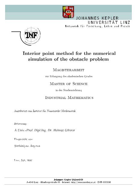
ÆØÞÛÖĐÙÖÓÖ×ÙÒ¸ÄÖÙÒÈÖÜ× ÂÇÀÆÆËÃÈÄÊ ÍÆÁÎÊËÁÌĐÌÄÁÆ<br />
ÁÒØÖÓÖÔÓÒØÑØÓÓÖØÒÙÑÖÐ ×ÑÙÐØÓÒÓØÓ×ØÐÔÖÓÐÑ<br />
ÞÙÖÖÐÒÙÒ×Ñ×ÒÖ× Å×ØÖÖØ<br />
Å×ØÖÓËÒ<br />
ÁÒÙ×ØÖÐÅØÑØ× ÒÖËØÙÒÖØÙÒ<br />
ÒÖØØÑÁÒ×ØØÙØĐÙÖÆÙÑÖ×ÅØÑØ<br />
ØÖÙÙÒ<br />
ÒÖØÚÓÒ ºÍÒÚº¹ÈÖÓºÔкÁÒºÖºÀÐÑÙØÖÖÖ<br />
ËÖÒÝÞÒÝÚ<br />
ÄÒÞ¸ÂÙи¾¼¼<br />
¹¼¼ÄÒÞ¡ÐØÒÖÖ×ØÖ¡ÁÒØÖÒØØØÔ»»ÛÛÛºÙÒ¹ÐÒÞººØ¡Îʼ¼¿ ÂÓÒÒ×ÃÔÐÖÍÒÚÖ×ØĐØ
Abstract<br />
In this work the interior point method is considered for the numerical solution<br />
of the obstacle problem. The scheme follows the predictor-corrector approach.<br />
For the numerical realization the unknowns are approximated by using first order<br />
finite elements. Results for several 2D examples are presented.
Contents<br />
Acknowledgments<br />
iii<br />
Introduction 1<br />
1 Mathematical modeling of the obstacle problem 2<br />
1.1 Statement of the problem . . . . . . . . . . . . . . . . . . . . . . 2<br />
1.2 Existence and uniqueness of the solution . . . . . . . . . . . . . . 3<br />
1.3 Alternative equivalent formulations . . . . . . . . . . . . . . . . . 6<br />
1.3.1 Variational inequality . . . . . . . . . . . . . . . . . . . . 6<br />
1.3.2 Free boundary problem . . . . . . . . . . . . . . . . . . . 8<br />
1.3.3 Linear complementarity problem . . . . . . . . . . . . . . 10<br />
2 Interior point method for the numerical solution of the obstacle problem<br />
11<br />
2.1 The central path . . . . . . . . . . . . . . . . . . . . . . . . . . . 11<br />
2.2 A predictor-corrector approach for the following the central path . 16<br />
2.2.1 The corrector step . . . . . . . . . . . . . . . . . . . . . 17<br />
2.2.2 The predictor step . . . . . . . . . . . . . . . . . . . . . 20<br />
3 Numerical implementation 23<br />
3.1 Algorithm . . . . . . . . . . . . . . . . . . . . . . . . . . . . . . 23<br />
3.2 Finite element discretization . . . . . . . . . . . . . . . . . . . . 26<br />
3.2.1 Corrector step . . . . . . . . . . . . . . . . . . . . . . . . 26<br />
3.2.2 Predictor step . . . . . . . . . . . . . . . . . . . . . . . . 29<br />
3.3 Error estimate for Finite Element solution . . . . . . . . . . . . . 29<br />
3.4 Numerical experiments . . . . . . . . . . . . . . . . . . . . . . . 32<br />
3.4.1 Example 1 . . . . . . . . . . . . . . . . . . . . . . . . . 33<br />
3.4.2 Example 2 . . . . . . . . . . . . . . . . . . . . . . . . . 35<br />
3.4.3 Example 3 . . . . . . . . . . . . . . . . . . . . . . . . . 38<br />
3.4.4 Example 4 . . . . . . . . . . . . . . . . . . . . . . . . . 40<br />
i
Conclusion 42<br />
A List of notations 43<br />
ii
Acknowledgments<br />
My sincere gratitude to my supervisor Prof. Helmut Gfrerer for his guidance and<br />
suggestions on this project work; especially, thanks for the providing me with<br />
the knowledge on the interior point method. I also want to thank the Computational<br />
Mathematics Institute for the challenging scientific atmosphere with their<br />
seminars.<br />
My special thanks to the Graduate School ”Mathematics <strong>as</strong> a Key Technology”<br />
of the Technical <strong>University</strong> of Kaiserslautern for their help in finding the sponsorship<br />
for my study. As a result I w<strong>as</strong> granted an Er<strong>as</strong>mus Mundus Scholarship for<br />
the participation in joint M<strong>as</strong>ter’s programme in Industrial Mathematics.<br />
In addition to my unforgettable and ple<strong>as</strong>ant impressions from staying in Europe,<br />
studying at the both universities, first year at the TU of Kaiserslautern and<br />
second year at the <strong>Johannes</strong> <strong>Kepler</strong> <strong>University</strong> of <strong>Linz</strong>, set up a solid scientific<br />
background me to be able to do this project work. Participation in this programme<br />
w<strong>as</strong> really great learning experience for me. I am grateful to all people who are<br />
involved in the organization of this nice programme for the given me opportunity<br />
to study in Europe and for the support and help during the study period.<br />
iii
Introduction<br />
The unknown of the obstacle problem is the deflection of the membrane which<br />
is stretched downward under an acting force and the deformation of which is restricted<br />
from below by an obstacle. Mathematically this problem can be posed<br />
<strong>as</strong> a constrained convex minimization problem, <strong>as</strong> a variational inequality, free<br />
boundary problem or <strong>as</strong> a linear complementarity problem. The mathematical<br />
formulations of this problem appears in many other applications: fluid filtration<br />
in porous media, el<strong>as</strong>to-pl<strong>as</strong>ticity, optimal control and financial mathematics.<br />
The formulations of the obstacle problem and existence of the solution have<br />
been discussed in many works e.g. by G.Stampacchia, L.A.Caffarelli, A.Friedman.<br />
Although there are results on the existence of the solution, it’s difficult to find the<br />
analytical solution in general c<strong>as</strong>e. That’s why the effective methods of the finding<br />
of numerical solution of this problem take important place in applications.<br />
In this work we consider an interior point method for the approximate solution<br />
of the obstacle problem. In chapter 1 we derive the mathematical model and<br />
discuss the existence and uniqueness of the solution. This chapter is b<strong>as</strong>ed mainly<br />
on the works [3] and [4]. In the chapter 2 we construct the interior point method<br />
for the obstacle problem when it’s considered <strong>as</strong> a minimization problem. In<br />
the third chapter the algorithm for the implementation is formulated. We use<br />
piecewise linear finite elements for the approximation of the solution. The part of<br />
this chapter about the finite element error estimate is b<strong>as</strong>ed on the work [8]. And,<br />
finally, we discuss numerical results of several examples.<br />
1
Chapter 1<br />
Mathematical modeling of the<br />
obstacle problem<br />
1.1 Statement of the problem<br />
We consider the membrane problem, when an el<strong>as</strong>tic membrane is attached to a<br />
flat wireframe and force is acting on it only in vertical direction. By Ω ⊂ R 2 we<br />
denote the domain which is enclosed by the wireframe. We denote by v(x,y) the<br />
deflection of the membrane. We choose the Cartesian coordinate system such that<br />
the Oxy plane coincides with the plane of the wireframe, so v(x,y) = 0 on ∂Ω. We<br />
<strong>as</strong>sume that the rigid body which we call ”the obstacle” in the following is placed<br />
under the membrane. Denoting by ψ(x,y) the surface of the obstacle we make<br />
<strong>as</strong>sumption that ψ(x,y) ≤ 0<br />
∀(x,y) ∈ ∂Ω.<br />
Total energy of the deformed membrane is :<br />
J(v) = P(v) − E(v),<br />
where P(v) - is the potential energy and E(v) is the energy due to the external<br />
forces. Assuming that the potential energy is proportional to the change of the<br />
membrane’s surface area we can approximate it by using of Taylor expansion:<br />
√<br />
∫<br />
P(v) = 1 + dv 2<br />
+ dv 2<br />
dω − µ(Ω) ≈ 1 ∫<br />
| ∇v | 2 dω,<br />
Ω dx dy<br />
2 Ω<br />
2
1.2 Existence and uniqueness of the solution 3<br />
here and in the following µ stays for the Lebesgue me<strong>as</strong>ure. Then the total energy<br />
is:<br />
J(v) = 1 2<br />
∫<br />
Ω<br />
∫<br />
| ∇v | 2 dω − f vdω.<br />
Ω<br />
The ”obstacle problem” consists in finding the equilibrium state of the membrane,<br />
i.e. in minimizing the energy functional J(v), when the deflection of the<br />
membrane is restricted from below by the obstacle. Then the set of admissible<br />
deflections is given <strong>as</strong> :<br />
K = {v ∈ H 1 0 (Ω)|v ≥ ψ a.e. in Ω}.<br />
We see that the K is not a linear set. Throughout this work we <strong>as</strong>sume that ψ ∈<br />
L 2 (Ω) and f ∈ H −1 (Ω).<br />
Thus, we come up with the following:<br />
Problem 1.1.1 Given a bounded domain Ω ⊂ R 2 and functions f ∈ H −1 andψ ∈<br />
L 2 (Ω), find a solution u ∈ H 1 0<br />
such that<br />
J(u) = minJ(v) ∀v ∈ K,<br />
v∈K<br />
where the functional J(v) : H0 1 → R is represented by :<br />
J(v) = 1 ∫<br />
|∇v| 2 dω − 〈 f ,v〉.<br />
2<br />
1.2 Existence and uniqueness of the solution<br />
Ω<br />
For the existence and uniqueness of the solution of the problem (1.1.1) we bring<br />
here the following statement for more general problem:<br />
Theorem 1.2.1 Let H be a Hilbert space, K ⊂ H be closed and convex, the continuous<br />
bilinear form a(·,·) : H × H → R be symmetric and coercive, i.e.<br />
∃α > 0 : a(v,v) ≥ α‖v‖ 2 v ∈ H,
1.2 Existence and uniqueness of the solution 4<br />
and f ∈ H ∗ .<br />
Then there exists unique solution to the minimization problem:<br />
to find u ∈ K : J(u) = minJ(v) ∀v ∈ K,<br />
v∈K<br />
where the functional J : H → R is defined by<br />
J(v) = 1 a(v,v) − 〈 f ,v〉.<br />
2<br />
Remark Here 〈 f ,v〉 is the pairing between f and v, i.e. 〈 f ,v〉 = f (v).<br />
Definition 1.2.2 The point y ∈ K such that<br />
‖x − y‖ ≤ ‖x − z‖ ∀z ∈ K<br />
is called the projection of x onto K.<br />
For the proof of the theorem we need the following lemma:<br />
Lemma 1.2.3 If K is closed and convex subset of a Hilbert space then each x ∈ H<br />
admits unique projection on K.<br />
Proof of the lemma (1.2.3) Let d = inf ‖x − z‖. Then we can find a sequence<br />
z∈K<br />
{η k } ∈ K : lim ‖η k − x‖ = d. Since K is convex, for any η m ,η n ∈ {η k } it holds<br />
k→∞<br />
1<br />
2<br />
(η m + η n ) ∈ K and<br />
d 2 ∥<br />
≤ ∥x − 1 2 (η m + η n ) ∥ 2 .<br />
Applying the parallelogram law for Hilbert space:<br />
2‖x − η m ‖ 2 + 2‖x − η n ‖ 2 = ‖η n − η m ‖ 2 ∥<br />
+ 2∥x − 1 2 (η n + η m ) ∥ 2 .<br />
Hence:<br />
‖η n − η m ‖ 2 ≤ 2‖x − η m ‖ 2 + 2‖x − η n ‖ 2 − 4d 2 .
1.2 Existence and uniqueness of the solution 5<br />
From this it follows that {η k } is Cauchy sequence, and since H is complete, it<br />
converges to an element y ∈ H. And, since K is closed, y ∈ K and ‖x − y‖ = d.<br />
Now, let’s suppose that there are two projections y 1 and y 2 of the element x.<br />
Then from the previous discussions it follows that :<br />
‖y 1 − y 2 ‖ 2 ≤ 2‖x − y 1 ‖ 2 + 2‖x − y 2 ‖ 2 − 4d 2 = 0.<br />
Therefore, y 1 = y 2 .<br />
Proof of the theorem (1.2.1) We can consider the bilinear form a(·,·) <strong>as</strong> the<br />
inner product in Hilbert space H, then the norm ‖v‖ a = √ a(v,v) is equivalent to<br />
the given norm in H. By the Riesz representation lemma we can find an element<br />
v ∗ ∈ H such that<br />
〈 f ,v〉 = a(v ∗ ,v) ∀v ∈ H.<br />
Then<br />
J(v) = 1 2 a(v,v) − a(v∗ ,v) = 1 2 ‖v − v∗ ‖ 2 a − 1 2 ‖v∗ ‖ 2 a.<br />
Thus, the problem of minimization of J(v) reduces to finding of the projection of<br />
v ∗ on the closed convex set K. By lemma (1.2.3) there exist unique projection,<br />
therefore unique solution of the minimization problem.<br />
To apply this theorem for the problem (1.1.1) we need to show respective<br />
∫<br />
properties of the set K and a(u,v) = ∇u∇vdω.<br />
Lemma 1.2.4 K is convex and closed.<br />
Ω<br />
Proof Let u,v ∈ K. Then for 0 < t < 1 : tu + (1 − t)v ∈ V and tu + (1 − t)v ≥<br />
tψ + (1 −t)ψ = ψ. This shows convexity of K.<br />
Now let {v k } ∈ K be a convergent sequence. Since from the convergence<br />
in V follows convergence in L 2 (Ω), it contains an a.e. pointwise convergent<br />
subsequence {v kn }. Let {v kn } −→ v pointwise. Suppose that v is not from K.
1.3 Alternative equivalent formulations 6<br />
Then there exist subset A ⊂ K : µ(A) > 0 such that v < ψ on A, more precisely,<br />
∃ε > 0 : v ≤ ψ − ε on A. But then<br />
∫<br />
Ω<br />
∫<br />
|v kn − v| 2 dxdy ≥<br />
A<br />
|v kn − v| 2 dxdy ≥ ε 2 µ(A) > 0.<br />
This contradicts to the above mentioned a.e. pointwise convergence. <br />
∫<br />
a(u,v) =<br />
Ω<br />
∇u∇vdω is bilinear and symmetric. It’s continuous:<br />
∫<br />
Ω<br />
∇u∇vdω ≤ |u| 1,Ω |v| 1,Ω ≤ ‖u‖ 1,Ω ‖v‖ 1,Ω ,<br />
and it’s coercitivity follows from Poincaré-Friedrichs inequality:<br />
∃C(Ω) > 0 : a(v,v) = |v| 2 1,Ω ≥ C(Ω)‖v‖2 1,Ω ∀v ∈ H1 0 .<br />
Thus, we have all prerequisites for the following statement:<br />
Theorem 1.2.5 Assume that ∃ ũ ∈ H 1 0<br />
solution ū to the problem (1.1.1).<br />
: ũ ≥ ψ a.e. in Ω. Then there exists unique<br />
1.3 Alternative equivalent formulations<br />
1.3.1 Variational inequality<br />
One of the most useful approaches to obtain the properties of the solution to the<br />
problem (1.1.1) is using its equivalent formulations by variational inequality. The<br />
problem (1.1.1) can be reformulated <strong>as</strong> follows:<br />
Problem 1.3.1 Let K ⊂ H 1 0 be closed and convex and f ∈ H−1 . To find:<br />
u ∈ K :<br />
∫<br />
Ω<br />
∇u∇(v − u)dω ≥ 〈 f ,v − u〉 ∀v ∈ K.<br />
Theorem 1.3.2 u ∈ K solves (1.1.1) if and only if it solves (1.3.1).
1.3 Alternative equivalent formulations 7<br />
Proof Let u ∈ K be the solution to the minimization problem (1.1.1). Then for<br />
t ∈ [0,1] : u+t(v−u) ∈ K ∀v ∈ K. Function defined by φ(t) = J(u+t(v−u)), t ∈<br />
[0,1] attains its minimum at the point t = 0, i.e.<br />
φ(0) ≤ φ(t) ∀t ∈ [0,1].<br />
Then<br />
∫<br />
φ(t) − φ(0)<br />
0 ≤ lim<br />
= ∇u∇(v − u)dω − 〈 f ,v − u〉.<br />
t→0+ t<br />
Ω<br />
∫<br />
Let u ∈ K be such that ∇u∇(v − u)dω ≥ 〈 f ,v − u〉 ∀v ∈ K. Then for any<br />
Ω<br />
v ∈ K it holds :<br />
∫<br />
J(v)−J(u) = φ(1)−φ(0) = ∇u∇(v−u)dω −〈 f ,v−u〉+ 1 ∫<br />
Ω 2<br />
<br />
The next theorem states about the well-posedness of the problem:<br />
Ω<br />
|∇(v−u)| 2 dω ≥ 0.<br />
Theorem 1.3.3 There exist unique solution to the problem (1.3.1). In addition,<br />
the mapping f → u is Lipschitz, that is, if u 1 ,u 2 are solutions to the problem<br />
(1.3.1) corresponding to f 1 , f 2 ∈ H −1 , then<br />
where L > 0 constant.<br />
‖u 1 − u 2 ‖ ≤ L‖ f 1 − f 2 ‖ H −1, (1.1)<br />
Proof Existence of the unique solution results from the previous discussions,<br />
namely, from the equivalence of the variational inequality (1.3.1) to the minimization<br />
problem (1.1.1).<br />
We demonstrate validity of (1.1). We set v = u 2 in the variational inequality<br />
for the solution u 1 and v = u 1 in the inequality for u 2 . Upon adding we obtain:<br />
∫<br />
|∇(u 1 − u 2 )| 2 dω ≤ 〈 f 1 − f 2 ,u 1 − u 2 〉.<br />
Ω<br />
From the coercitivity of the form a(u,v) = ∫ Ω ∇u∇vdω, it follows that<br />
C(Ω)‖u 1 − u 2 ‖ 2 ≤ 〈 f 1 − f 2 ,u 1 − u 2 〉 ≤ ‖ f 1 − f 2 ‖ H −1‖u 1 − u 2 ‖.
1.3 Alternative equivalent formulations 8<br />
1.3.2 Free boundary problem<br />
Now we <strong>as</strong>sume that u ∈ H 2 (Ω) ∩ K is the solution of the obstacle problem. We<br />
divide domain Ω into the set Ω + = {x ∈ Ω : u(x) > ψ(x)}, which we call noncoincidence<br />
set, and coincidence set Ω 0 = {x ∈ Ω : u(x) = ψ(x)}.<br />
Since u solves the variational inequality (1.3.1), applying Green’s formula to<br />
the left hand side of the inequality we obtain<br />
∫<br />
∫<br />
∂u<br />
− ∆u(v − u)dω +<br />
Ω<br />
∂Ω ∂n<br />
∫Ω<br />
(v − u)ds ≥ f (v − u)dω ∀v ∈ K. (1.2)<br />
Both u,v ∈ K ⊂ H0 1 , so the boundary term vanishes. Let’s take any nonnegative<br />
function ζ ∈ C0 ∞ (Ω). Then v = u+εζ ∈ K for ε ≥ 0. Substituting this in the latter<br />
inequality, we obtain:<br />
From this it follows that :<br />
∫<br />
∫<br />
− ∆uζ dω ≥ f ζ dω, ∀ζ ∈ C0 ∞ , ζ ≥ 0.<br />
Ω<br />
Ω<br />
−∆u ≥ f a.e. in Ω.<br />
Let’s <strong>as</strong>sume that ψ ∈ C(Ω). Then the set Ω + is open, since u ∈ H 2 ↩→ C(Ω).<br />
We consider a point x ∈ Ω + , for which we can choose a neighborhood U δ (x)<br />
such that U δ (x) ⊂ Ω + . For any ζ ∈ C ∞ 0 (U δ (x)) we may find an ε > 0 such that<br />
v = u + εζ ∈ K. Substituting this v in (1.2) and dividing by ε we find that<br />
∫<br />
∫<br />
− ∆uζ dω ≥ f ζ dω<br />
U δ (x)<br />
U δ (x)<br />
In particular this holds for −ζ , therefore<br />
and also a.e. in Ω + .<br />
−∆u = f in U δ (x),<br />
∀ζ ∈ C ∞ 0 (U δ (x).)<br />
The function u − ψ ∈ H 2 (Ω), where u ∈ K is the solution of the obstacle<br />
problem, attains its minimum in Ω in the coincidence set Ω 0 . Thus, using the
1.3 Alternative equivalent formulations 9<br />
Figure 1.1: Free boundary for 1D problem.<br />
necessary condition for extremal point, we have then:<br />
u = φ on Γ ∗ ,<br />
∇u = ∇φ on Γ ∗ ,<br />
where Γ ∗ = ∂Ω + ∩ Ω is called the free boundary of the problem.<br />
We have shown that the solution of the obstacle problem with the appropriate<br />
data corresponds to the formal solution of the following boundary problem:<br />
⎧<br />
−∆u ≥ f a.e. in Ω,<br />
u ≥ ψ a.e. in Ω,<br />
⎪⎨<br />
if u(x) > ψ(x) then − ∆u(x) = f (x),<br />
u = φ on Γ ∗ ,<br />
∇u = ∇φ on Γ ⎪⎩<br />
∗ ,<br />
u = 0 on ∂Ω.<br />
Note that the free boundary of the problem is not known in advance. This kind<br />
of formulations may be useful only in the one-dimensional c<strong>as</strong>e of the problem,<br />
since we don’t know about the smoothness of the Γ ∗ .
1.3 Alternative equivalent formulations 10<br />
1.3.3 Linear complementarity problem<br />
We can reformulate the free boundary problem so that the free boundary conditions<br />
need not be handled explicitly <strong>as</strong> follows:<br />
⎧<br />
⎪⎨<br />
⎪⎩<br />
−∆u ≥ f a.e. in Ω,<br />
u ≥ ψ a.e. in Ω,<br />
(u − ψ)(−∆u − f ) = 0 a.e. in Ω,<br />
u = 0<br />
on ∂Ω.<br />
(1.3)<br />
Some results for this form of the obstacle problem interested reader can find<br />
in the work of Brézis and Stampacchia: if f ∈ L 2 (Ω), and ψ ∈ H 2 (Ω) then the<br />
problem (1.3.1) h<strong>as</strong> a unique solution u ∈ H 2 (Ω) and it satisfies (1.3).
Chapter 2<br />
Interior point method for the<br />
numerical solution of the obstacle<br />
problem<br />
2.1 The central path<br />
The idea of the interior point methods is to replace the constrained minimization<br />
problem by a sequence of unconstrained minimization problems, for solving of<br />
which we can use Newton’s method. An objective functional of the unconstrained<br />
problem we generate by adding barrier functional to the objective functional of the<br />
original constrained problem. Barrier function serves <strong>as</strong> barrier against leaving of<br />
the elements the fe<strong>as</strong>ible region K. Each of the problems in the sequence corresponds<br />
to the objective functional J κ (v) depending on the nonnegative penalty<br />
parameter κ. For our problem we construct J κ (v) in the following way:<br />
∫<br />
J κ (v) = J(v) − κ ln(v − ψ)dω.<br />
Ω<br />
We extend the definition of the ln to the whole real domain axis by setting lnz =<br />
−∞,<br />
z ≤ 0. Then barrier function approaches infinity <strong>as</strong> the elements from the<br />
interior approach the boundary. Thus we obtained the family of the following<br />
unconstrained minimization problem:<br />
11
2.1 The central path 12<br />
Problem 2.1.1 Given a bounded domain Ω ⊂ R 2 and functions f ∈ H −1 andψ ∈<br />
L 2 (Ω), find a solution u κ ∈ H0 1 (Ω) such that<br />
J κ (u κ ) =<br />
min<br />
v∈H 1 0 (Ω) J κ (v)<br />
∀v ∈ H 1 0 (Ω),<br />
where the functional J κ (v) : H 1 0<br />
→ R is represented by :<br />
J κ (v) = 1 2<br />
∫<br />
Ω<br />
∫<br />
|∇v| 2 dω − 〈 f ,v〉 − κ ln(v − ψ).<br />
Ω<br />
Now we will determine the existence and uniqueness of the solution for the auxiliary<br />
problems (2.1.1). We use the following theorem:<br />
Theorem 2.1.2 Let V be a Hilbert space and let F : V → R ∪ {±∞} be a proper<br />
lower semicontinuous function. If F is coercive, i.e. that<br />
then the problem<br />
lim F(u) = ∞,<br />
‖u‖→∞<br />
min F(u)<br />
u∈V<br />
h<strong>as</strong> at le<strong>as</strong>t one solution. If F is strictly convex, then the solution is unique.<br />
Proof Let {u n } ∈ V be the minimizing sequence :<br />
Since c < +∞ and F(u) is coercive:<br />
c = lim<br />
n→∞<br />
F(u n ) = inf<br />
u∈V F(u).<br />
‖u n ‖ < const.<br />
Then we can find subsequence {u nk } ⊂ {u n } weakly converging in V :<br />
u nk ⇀ ū ∈ V.
2.1 The central path 13<br />
By virtue of lower semicontinuity of F(u):<br />
Then it holds that<br />
so u = ū is the solution to the problem.<br />
lim F(u n) ≥ F(ū).<br />
n→∞<br />
F(ū) ≤ inf<br />
u∈V F(u),<br />
Let now u 1 ,u 2 ∈ V be two solutions to the problem. Then 1 2 (u 1 + u 2 ) ∈ V. If<br />
F(u) is strictly convex function, then<br />
( )<br />
1<br />
F<br />
2 (u 1 + u 2 )<br />
< min<br />
u∈V F(u),<br />
so only one solution exists for the strictly convex F(u). <br />
We make an <strong>as</strong>sumption (A1):<br />
∃ũ ∈ H 1 0 (Ω) :<br />
∫<br />
− ln(ũ − ψ)dω < ∞.<br />
Ω<br />
Theorem 2.1.3 With the <strong>as</strong>sumption (A1) for each κ > 0 the problem (2.1.1) h<strong>as</strong><br />
a unique solution u κ .<br />
Proof Let κ > 0 be an arbitrary fixed number. We apply theorem 2.1.2 with<br />
V = H0 1(Ω) and F(u) = J κ(u). J κ (u) is the sum of the strictly convex continuous<br />
∫<br />
function J(u) and the function φ(u) = − ln(u − ψ)dω. It’s clear that φ(u) is a<br />
convex function and consequently J κ (u) is strictly convex. Using the inequality<br />
lnz ≤ z for z > 0 we obtain<br />
∫<br />
φ(u) ≥ − max{u − ψ,0} ≥ −‖u − ψ‖ L 2 (Ω) µ(Ω) 1 2 .<br />
Ω<br />
Since ‖u − ψ‖ ≥ ‖u − ψ‖ L 2 (Ω), together with the <strong>as</strong>sumption (A1) it follows that<br />
φ and hence also J κ is proper. Moreover, we obtain<br />
J κ (u) ≥ c‖u‖ 2 − ‖ f ‖‖u‖ − κ‖u − ψ‖µ(Ω) 1 2<br />
Ω
2.1 The central path 14<br />
for some c > 0. Hence<br />
lim J κ(u) = ∞<br />
‖u‖→∞<br />
follows. It remains to show lower semicontinuity of J κ . It suffices to show that φ<br />
is lower semicontinuous.<br />
From the definition of the Lebesgue integral,<br />
φ(u) = supφ ε (u)<br />
ε>0<br />
∫<br />
follows, where φ ε (u) = − ln(max{u − ψ,ε})dω. Since the pointwise supremum<br />
of a family of continuous functions is lower semicontinuous, lower<br />
Ω<br />
semicontinuity<br />
of φ follows. <br />
Definition 2.1.4 The mapping κ → u κ is called the central path.<br />
The idea behind the interior point method is to follow the central path. This<br />
means we begin with some value of κ and find the solution to the corresponding<br />
unconstrained problem. Then we decre<strong>as</strong>e κ and solve again the auxiliary problem,<br />
and so on. Next theorem states about the convergence of u κ to ū <strong>as</strong> κ → 0.<br />
Theorem 2.1.5 For all κ > 0 one h<strong>as</strong> J(u κ ) ≤ J(ū) + κµ(Ω).<br />
∫<br />
Proof We denote again by φ(u) = − ln(u − ψ)dω.<br />
Ω<br />
For fixed κ > 0, let η(t) = J κ (v t ) for t ∈ [0,1), where v t = tū + (1 − t)u κ .<br />
Since<br />
v t − ψ = t(ū − ψ) + (1 −t)(u κ − ψ) ≥ (1 −t)(u κ − ψ) ≥ 0 a.e. in Ω,<br />
together with the monotonicity of ln, we have η(0) ≤ η(t) ≤ J(v t ) + κφ(u κ ) −<br />
κ ln(1 − t)µ(Ω) < +∞, t ∈ [0,1). It’s e<strong>as</strong>y to see that η(t) is convex on [0,1).
2.1 The central path 15<br />
Then the function θ(t) = η(t)−η(0)<br />
t<br />
from below by 0. Hence there exists<br />
Further we have<br />
∫<br />
0 ≤ η ′ (0) =<br />
It also follows<br />
is monotone nondecre<strong>as</strong>ing and it’s bounded<br />
η ′ η(t) − η(0)<br />
(0) = lim<br />
≥ 0, t ∈ (0,1).<br />
t→0+ t<br />
Ω<br />
φ(v t ) − φ(v 0 )<br />
t<br />
φ(v t ) − φ(0)<br />
∇u κ ∇(ū − u κ )dω + 〈 f ,ū − u κ 〉 + κ lim<br />
.<br />
t→0 t<br />
∫<br />
= κ t −1 (ln(v 0 − ψ) − ln(v t − ψ))dω.<br />
Ω<br />
As t → 0, the integrand converges to u κ−ū<br />
u κ −ψ a.e. in Ω. Further, on the set {u κ ≥<br />
ū} we have<br />
0 ≤ t −1 (ln(v 0 − ψ) − ln(v t − ψ)) ≤ u κ − ū<br />
v t − ψ ≤ u κ − ψ<br />
v t − ψ ≤ 1<br />
1 −t ,<br />
and hence, by theorem of dominated convergence, we obtain<br />
∫<br />
∫<br />
lim t −1 u κ − ū<br />
(ln(v 0 − ψ) − ln(v t − ψ))dω =<br />
t→0+ {u κ ≥ū}<br />
{u κ ≥ū} u κ − ψ dω.<br />
On the other hand, on the set u κ < ū we have<br />
t −1 (ln(v 0 − ψ) − ln(v t − ψ)) ↘ u κ − ū<br />
u κ − ψ<br />
< 0, for t → 0 + .<br />
Since<br />
∫<br />
lim<br />
t→0+ {u κ
2.2 A predictor-corrector approach for the following the central path 16<br />
∫<br />
by the theorem of Beppo-Levi. Hence,<br />
∫<br />
0 ≤ η ′ (0) =<br />
Ω<br />
Ω<br />
u κ − ū<br />
dω exists and<br />
u κ − ψ<br />
∫<br />
u κ − ū<br />
∇u κ ∇(ū − u κ )dω + 〈 f ,ū − u κ 〉 + κ<br />
Ω u κ − ψ dω.<br />
It follows that t = 0 is the solution of the optimization problem<br />
Therefore,<br />
∫<br />
min J(v u κ − ū<br />
t) + κt<br />
t≥0 Ω u κ − ψ dω.<br />
∫<br />
J(v 0 ) ≤ J(v 1 ) + κ 1 − ū − ψ<br />
Ω u κ − ψ dω ≤ J(v 1) + κµ(Ω)<br />
and since v 0 = u κ , v 1 = ū, the theorem is proved. <br />
Using in this inequality Taylor expansion of J(u κ ) at the point ū, we obtain:<br />
or, equivalently,<br />
∫<br />
1<br />
|∇(u κ − ū)| 2 dω ≤ κµ(Ω),<br />
2 Ω<br />
‖u κ − ū‖ H 1<br />
0 (Ω) = O(√ κ).<br />
2.2 A predictor-corrector approach for the following<br />
the central path<br />
All the results from the preceding section remain valid if we replace H0 1 (Ω) by a<br />
closed subspace V ⊂ H0 1(Ω), e.g. if ∃ ũ ∈ V : ∫ Ω ln(ũ − ψ)dω < ∞ then for each<br />
κ > 0 the problem<br />
min J κ(v) ∀v ∈ V,<br />
v∈V<br />
with<br />
J κ (v) = 1 2<br />
∫<br />
Ω<br />
∫<br />
|∇v| 2 dω − 〈 f ,v〉 − κ ln(v − ψ),<br />
Ω<br />
h<strong>as</strong> a unique solution which is again denoted by u κ .
2.2 A predictor-corrector approach for the following the central path 17<br />
2.2.1 The corrector step<br />
For given κ > 0 we are given an approximation u ∈ V of u κ and we want to find<br />
a better approximation u + by means of Newton’s method, i.e. u + = u + δu where<br />
the so called Newton corrector δu is a solution of the problem<br />
with<br />
min φ κ,u(v) (2.1)<br />
v∈V<br />
φ κ,u (v) = J κ (u) + J κ(u)v ′ + 1 2 J′′ κ(v,v).<br />
Here J ′ κ(u) : V → R, and J ′′<br />
κ(u) : V ×V → R are<br />
and<br />
∫<br />
J κ(u)v ′ =<br />
Ω<br />
∫<br />
v<br />
∇u∇vdω − 〈 f ,v〉 − κ<br />
Ω u − ψ dω<br />
∫<br />
∫<br />
J κ(u)(v,w) ′′<br />
vw<br />
= ∇v∇wdω + κ<br />
Ω<br />
Ω (u − ψ) 2 dω.<br />
For e<strong>as</strong>e of presentation we <strong>as</strong>sume that u − ψ ≥ ε > 0 a.e. in Ω. Then J ′ (u) and<br />
J ′′ (u) are well defined. Further, it e<strong>as</strong>ily follows that φ κ,u is a continuous strictly<br />
convex functional on V and a unique minimizer δu of φ κ,u exists and satisfies<br />
J ′′<br />
κ(u)(δu,v) = −J ′ κ(u)v, ∀v ∈ V.<br />
So at this step we replaced the objective functional J κ by its quadratic approximation<br />
φ κ,u . Since we used the logarithmic barrier functions it’s sufficient here<br />
to use Taylor expansion up to the second order. Thus we can rely on Newton’s<br />
method for solving this problem.<br />
Now let us analyze the next corrector step given by the unique solution δu +<br />
of the optimization problem<br />
min φ κ,u +(v).<br />
v∈V
2.2 A predictor-corrector approach for the following the central path 18<br />
Since<br />
J ′ κ(u + )v =<br />
we obtain<br />
∫<br />
Ω<br />
∫<br />
∇u + ∇vdω − 〈 f ,v〉 − κ<br />
= J ′ κ(u)v + J ′′<br />
κ(u)(δu,v) − κ<br />
∫<br />
= −κ<br />
Ω<br />
Ω<br />
∫<br />
Ω<br />
(δu) 2 v<br />
(u + − ψ)(u − ψ) 2 dω<br />
v<br />
u + − ψ dω<br />
( v<br />
u + − ψ −<br />
v<br />
u − ψ +<br />
δu v )<br />
(u − ψ) 2 dω<br />
∫<br />
J κ(u ′′ + )(δu + ,v) = −J κ(u ′ + (δu) 2 v<br />
)v = κ<br />
Ω (u + dω, ∀v ∈ V.<br />
− ψ)(u − ψ)<br />
By taking v = δu + it follows that<br />
and<br />
∫<br />
Ω<br />
∫<br />
|∇δu + | 2 dω + κ<br />
Ω<br />
(δu + ) 2<br />
(u + − ψ) 2 dω = κ ∫Ω<br />
Using the Cauchy-Schwartz inequality we conclude that<br />
∫<br />
κ<br />
Ω<br />
(δu + ) 2<br />
(u + − ψ) 2 dω ≤ κ ( ∫<br />
Ω<br />
∫<br />
Ω<br />
(δu + ) 2<br />
(u + − ψ) 2 dω ) 1<br />
2<br />
( ∫<br />
Ω<br />
δu + (δu) 2<br />
(u + dω. (2.2)<br />
− ψ)(u − ψ) 2<br />
(δu) 4<br />
(u − ψ) 4 dω ) 1<br />
2<br />
(δu + ) 2<br />
(u + − ψ)<br />
∫Ω<br />
2 dω ≤ (δu) 4<br />
dω. (2.3)<br />
(u − ψ) 4<br />
Now consider Newton’s step defined by u n+1 = u n +δu n , n = 0,1,2,..., where<br />
δu n is the unique minimizer of φ κ,u n(·).<br />
Definition 2.2.1 We say the sequence {γ n } converges R-superlinearly to γ if<br />
√<br />
n<br />
lim ‖γ n − γ‖ = 0.<br />
n→∞<br />
Theorem 2.2.2 Let κ > 0 be fixed and <strong>as</strong>sume that there exist some reals C > 0<br />
such that<br />
∥ δu<br />
∥ ∥∥<br />
∥<br />
u − ψ<br />
≤ C δu<br />
∥<br />
L ∞ (Ω) u − ψ<br />
∥<br />
L 2 (Ω)<br />
∀u > ψ.<br />
Then for all starting points u 0 > ψ with ‖ δu0<br />
u 0 −ψ ‖ L 2 (Ω) < C 1 Newton iterations converge<br />
to u κ . Moreover, the convergence is R-superlinear.
2.2 A predictor-corrector approach for the following the central path 19<br />
Proof From (2.3) we obtain<br />
∥ δun+1<br />
∥ ∥∥<br />
u n+1 ∥<br />
− ψ<br />
≤ δu n<br />
L 2 (Ω) u n ∥ ∥ δun<br />
∥ ∥∥<br />
− ψ L ∞ (Ω) u n ∥<br />
− ψ<br />
≤ C δu n<br />
L 2 (Ω) u n ∥ 2<br />
− ψ<br />
.<br />
L 2 (Ω) With the starting point ∥ δu0<br />
∥ < τ L 2 (Ω)<br />
C<br />
, 0 < τ < 1 it follows then<br />
u 0 −ψ<br />
From (2.2) we obtain for ∇δu n+1<br />
∫<br />
Ω<br />
∥ δun<br />
u n ∥<br />
− ψ<br />
< τ2n<br />
L 2 (Ω) C .<br />
∫<br />
|∇δu n+1 | 2 δu n+1 (δu n ) 2<br />
≤ κ<br />
Ω (u n+1 − ψ)(u n − ψ) 2 dω<br />
∥<br />
⇒ |δu n+1 | 2 ∥∥<br />
1,Ω ≤ κ δu n+1<br />
∥<br />
u n+1 − ψ<br />
√ κ<br />
⇒ |δu n+1 | 1,Ω ≤<br />
C τ2n+1<br />
∥<br />
L 2 (Ω)<br />
∥ δun<br />
∥<br />
u n − ψ<br />
∥<br />
L 2 (Ω)<br />
∥ δun<br />
∥<br />
u n − ψ<br />
∥<br />
L ∞ (Ω)<br />
This implies that ‖δu n+1 ‖ → 0 <strong>as</strong> n → ∞, so the sequence {u n } is Cauchy sequence<br />
and it converges to some element ū ∈ V :<br />
Due to the strict convexity of J κ it holds:<br />
Consider J ′ κ(u n )(v − u n ) :<br />
ū = lim<br />
n→∞<br />
u n .<br />
J κ (v) ≥ J κ (u n ) + J ′ κ(u n )(v − u n ) ∀v ∈ V. (2.4)<br />
J κ(u ′ n )(v − u n ) = −J κ(δu ′′ n ,v − u n )<br />
∫<br />
∫<br />
= ∇δu n ∇(v − u n δu n (v − u n )<br />
) + κ<br />
Ω<br />
Ω (u n − ψ) 2<br />
≤ |δu n | 1,Ω ‖v − u n ‖ 1,Ω + κ∥ δun<br />
u n ∥ ∥ v − un<br />
− ψ L 2 (Ω) u n ∥<br />
− ψ<br />
.<br />
L 2 (Ω)<br />
From this we can conclude that J ′ κ(u n )(v − u n ) → 0 <strong>as</strong> n → ∞. Taking the limit in<br />
(2.4) we obtain<br />
J(v) ≥ J(ū) ∀v ∈ V,
2.2 A predictor-corrector approach for the following the central path 20<br />
thus ū = u κ .<br />
It remains to justify R-superlinear convergence:<br />
|u n ∞<br />
√ κ<br />
− ū| 1,Ω ≤ ∑ |δu k ∞<br />
√ κ τ<br />
| 1,Ω ≤<br />
k=n<br />
C<br />
∑<br />
2n<br />
τ 2k ≤<br />
k=n<br />
C 1 − τ 2 .<br />
Consequently,<br />
<br />
√<br />
n<br />
lim ‖u n − ū‖ = 0.<br />
n→∞<br />
2.2.2 The predictor step<br />
For κ > 0 let u + = u + δu be the result of one corrector step. Under the <strong>as</strong>sumptions<br />
of theorem 2.2.2 u + is sufficiently near u κ , when ∥ u−ψ<br />
δu<br />
∥ ≤ τ L 2 (Ω)<br />
C<br />
for some<br />
τ < 1.<br />
Now we want to approximate u κ + for the smaller penalty parameter κ + =<br />
(1 − ρ)κ. To do this we compute a predictor p <strong>as</strong> the unique solution of the minimization<br />
problem<br />
min<br />
v∈V J(u+ ) + J ′ (u + )v + 1 2 J′′ κ(u + )(v,v) (2.5)<br />
and take ũ = u + + ρ p <strong>as</strong> starting point for the next Newton’s method to approximate<br />
u κ +. We want to stay near the central path by performing single Newton’s<br />
step. For a given accuracy of the Newton method τ, in view of theorem 2.2.2 we<br />
want to choose ρ such that the next corrector δũ satisfies<br />
∥ δũ<br />
∥<br />
ũ − ψ<br />
≤ τ L 2 (Ω) C .<br />
We present now an analysis for a proper choice of ρ. As the solution to the minimization<br />
problem (2.5) the predictor p satisfies<br />
J ′′<br />
κ(u + )(p,v) = −J ′ (u + )v ∀v ∈ V. (2.6)
2.2 A predictor-corrector approach for the following the central path 21<br />
And for the next corrector step it holds<br />
We have<br />
J ′′<br />
κ(ũ)(δũ,v) = −J ′ κ(ũ)v ∀v ∈ V. (2.7)<br />
∫<br />
J ′ (ũ)v = J ′ (u + )v + ρ ∇p∇vdω ∀v ∈ V,<br />
Ω<br />
then by use of (2.6) we obtain<br />
(<br />
∫<br />
∀v ∈ V J ′ (ũ)v = J ′ (u + )v + ρ −J ′ (u + )v − κ<br />
∫<br />
= (1 − ρ)J ′ (u + )v − ρκ<br />
Ω<br />
(<br />
∫<br />
= (1 − ρ) J κ(u ′ + )v + κ<br />
=<br />
and consequently, denoting by ξ = δu<br />
u−ψ ,:<br />
∀v ∈ V − J ′ κ + (ũ)v = −J ′ (ũ)v + κ + ∫<br />
∫<br />
Ω<br />
=<br />
=<br />
=<br />
Ω<br />
pv<br />
(u + − ψ) 2<br />
Ω<br />
)<br />
pv<br />
(u + − ψ) 2 dω<br />
)<br />
v<br />
u + − ψ dω − ρκ<br />
∫<br />
Ω<br />
pv<br />
(u + − ψ) 2<br />
−κ + (δu) 2 v<br />
(u + − ψ)(u − ψ) 2 + v<br />
κ+<br />
u + − ψ − ρκ pv<br />
(u + − ψ) 2 dω<br />
∫<br />
Ω<br />
∫<br />
κ +<br />
Ω<br />
∫<br />
κ +<br />
Ω<br />
Ω<br />
( ξ<br />
κ + 2 v<br />
u + − ψ −<br />
v<br />
ũ − ψ dω<br />
v<br />
u + − ψ +<br />
v )<br />
ũ − ψ<br />
pv<br />
+ ρκ<br />
(u + − ψ) 2 dω<br />
ξ 2 v<br />
u + − ψ − pv<br />
ρκ+ (u + − ψ)(ũ − ψ) + ρκ pv<br />
(u + − ψ) 2 dω<br />
ξ 2 v<br />
u + − ψ + ρ2 κ p(u+ + p − ψ)v<br />
(u + − ψ) 2 (ũ − ψ) dω.<br />
Then using (2.7) with v = δũ and application of the Cauchy-Schwartz inequality<br />
yield<br />
∫<br />
Ω<br />
|∇δũ| 2 dω + κ + ∫<br />
Ω<br />
(δũ) 2 ( ∫<br />
(ũ − ψ) 2 dω ≤ (δũ) 2 ) 1<br />
2 κ+ Ξ<br />
Ω (ũ − ψ) 2 dω ,<br />
where<br />
∫<br />
Ξ =<br />
Ω<br />
(<br />
ξ 2 p<br />
(1 + ρ<br />
u + − ψ ) +<br />
ρ2<br />
1 − ρ<br />
(<br />
p<br />
u + 1 + p )) 2<br />
− ψ u + dω.<br />
− ψ
2.2 A predictor-corrector approach for the following the central path 22<br />
It follows then<br />
∫<br />
Ω<br />
(δũ) 2<br />
dω ≤ Ξ.<br />
(ũ − ψ) 2<br />
Thus we constructed a policy for a choice of a suitable decre<strong>as</strong>ing parameter ρ for<br />
κ: ρ should satisfy the following conditions<br />
1. ρ < 1<br />
2. u + − ψ + ρ p > 0 in Ω<br />
3. Ξ ≤ ( τ<br />
C<br />
) 2 .
Chapter 3<br />
Numerical implementation<br />
3.1 Algorithm<br />
Interior point method consists of outer cycle : corrector-predictor steps and inner<br />
cycle for solely corrector step. As starting point for the approximate solution we<br />
can choose u h = 0.<br />
As we already noted the principle of the interior point method is to follow the<br />
central path. Ideally, we would like the iterations u i corresponding to κ i would<br />
lie on the central path, i.e. u i = u κi , where u κi is the exact solution of the corresponding<br />
UP. But to achieve high accuracy on each corrector step would cost us<br />
a number of iterations. So, instead, we try our approximate solutions in each corrector<br />
step to remain in the predefined neighborhood of the exact solution (picture<br />
3.1).<br />
∥<br />
Under the <strong>as</strong>sumption that<br />
we have:<br />
∥ δun+1<br />
∥<br />
u n+1 − ψ<br />
∥<br />
L ∞ (Ω)<br />
∥ δu0<br />
u 0 −ψ<br />
≤<br />
≤<br />
≤<br />
∥ < τ L 2 (Ω)<br />
C<br />
, from the proof of theorem 2.2.2<br />
C∥ δun+1<br />
∥<br />
u n+1 − ψ<br />
C∥ δun<br />
∥<br />
u n − ψ<br />
τ 2n∥ ∥ δu n<br />
∥<br />
u n − ψ<br />
∥<br />
L 2 (Ω)<br />
∥<br />
L ∞ (Ω)<br />
∥<br />
L ∞ (Ω)<br />
∥ δun<br />
∥<br />
u n − ψ<br />
∥<br />
L 2 (Ω)<br />
23
3.1 Algorithm 24<br />
Figure 3.1: Staying close to the central path by single Newton iterations<br />
Thus, if we choose at each predictor step decre<strong>as</strong>ing factor ρ of the κ such that<br />
the starting point ũ for the next Newton iterations satisfies ∥ ũ−ψ<br />
δũ<br />
∥ < τ L 2 (Ω)<br />
C and<br />
∥ ∥<br />
define to stop Newton iterates <strong>as</strong> the condition<br />
< τ is satisfied, then<br />
∥ u−ψ<br />
δu ∥<br />
L 2 (Ω)<br />
we reach this kind of accuracy τ for the corrector step just in single step:<br />
∥ δu1<br />
∥ ∥∥<br />
u 1 ∥<br />
− ψ<br />
≤ C δu 0<br />
∥<br />
L ∞ (Ω) u 0 − ψ<br />
∥<br />
L ∞ (Ω)<br />
∥ δu0<br />
∥<br />
u 0 − ψ<br />
∥<br />
L 2 (Ω)<br />
≤ C2<br />
τ2<br />
C 2 < τ.<br />
We also need to determine the constant C for the <strong>as</strong>sumptions of the theorem<br />
2.2.2 to be fulfilled. This constant can be found by updating it at each Newton<br />
∥ ∥<br />
∥∥<br />
iterate <strong>as</strong> the maximal value of the old one and the ratio ∥ / δu<br />
∥ .<br />
L ∞ (Ω) L 2 (Ω)<br />
∥ u−ψ<br />
δu<br />
After solving of the elliptic equations for the corrector δu we need to choose<br />
the step-size α such that updated value of the approximate solution would be fe<strong>as</strong>ible,<br />
i.e. it should hold u + αδ > ψ. This is equivalent to α<br />
u−ψ δu > −1, and since<br />
under the appropriate <strong>as</strong>sumptions ∥ u−ψ<br />
δu<br />
∥ ≤ τ holds, for the implementation<br />
L ∞ (Ω)<br />
∥<br />
we write it <strong>as</strong> ∥α δu<br />
∥ < 1.<br />
L ∞ (Ω)<br />
u−ψ<br />
u−ψ
3.1 Algorithm 25<br />
Algorithm 1 Interior points method<br />
1: precision ε, precision τ, κ, u (0)<br />
2: k=0<br />
3: repeat<br />
4: u ← u (k)<br />
5: repeat<br />
6: solve for { δu : J κ(u)(δu,v) ′′ = −J ∥ κ(u)v<br />
′ 7: C = max C, ∥ δu<br />
∥∥<br />
∥ / δu ∥<br />
L ∞ (Ω)<br />
u−ψ<br />
u−ψ ∥<br />
L 2 (Ω)<br />
8: choose step-size 0 < α ≤ 1 such that :<br />
} ∀v ∈ V<br />
∥<br />
∥α δu<br />
u−ψ<br />
∥ ≤ 0.99<br />
L ∞ (Ω)<br />
9: u = u + αδu<br />
10: until ‖<br />
u−ψ δu ‖ L ∞ (Ω) ≤ τ<br />
11: solve for a predictor p : J κ(u)(p,v) ′′ = −J ′ (u)v, ∀v ∈ V.<br />
12: choose 0 < ρ < 0.99 such that :<br />
∥<br />
• ∥ρ δu<br />
∥ ≤ 0.99<br />
L ∞ (Ω)<br />
u−ψ<br />
• Ξ ≤ ( τ<br />
C<br />
) 2<br />
13: κ = (1 − ρ)κ<br />
14: k=k+1<br />
15: u (k+1) = u + ρ p<br />
16: until κ ≤ ε<br />
As we established in the preceding section we also need choose the step-size<br />
ρ for the predictor such that the condition<br />
with<br />
∫<br />
Ξ =<br />
Ω<br />
( ( ) δu 2 (<br />
1 + ρ<br />
u − ψ<br />
p<br />
u + − ψ<br />
( τ 2<br />
Ξ ≤<br />
C)<br />
)<br />
+ ρ2<br />
1 − ρ<br />
(<br />
p<br />
u + 1 + p ) ) 2<br />
− ψ u + dω<br />
− ψ<br />
(3.1)<br />
would be satisfied. For realization of this condition we set the ρ = 0.99, and then<br />
decre<strong>as</strong>e it consecutively until it’s appropriate. For the saving of the computation
3.2 Finite element discretization 26<br />
time it makes sense to divide the integral (3.1) into the several parts <strong>as</strong> follows:<br />
Ξ = I 1 + 2ρI 2 + ρ 2 I 3 + 2 ρ2<br />
1 − ρ I 4 + 2ρ ρ2<br />
1 − ρ I 5 + ρ4<br />
(1 − ρ) 2 I 6,<br />
where<br />
I 1 =<br />
I 2 =<br />
I 3 =<br />
I 4 =<br />
I 5 =<br />
I 6 =<br />
∫<br />
Ω<br />
∫<br />
Ω<br />
∫<br />
Ω<br />
∫<br />
Ω<br />
∫<br />
Ω<br />
∫<br />
Ω<br />
( ) δu 4<br />
dω<br />
u − ψ<br />
( ) δu 4<br />
p<br />
u − ψ u + − ψ dω<br />
( ) δu 4 ( ) p 2<br />
u − ψ u + dω<br />
− ψ<br />
( ) δu 2 (<br />
p<br />
u − ψ u + 1 + p )<br />
− ψ u + dω<br />
− ψ<br />
( ) δu 2 ( ) p 2 (<br />
u − ψ u + 1 + p<br />
− ψ u + − ψ<br />
) 2<br />
dω<br />
( p<br />
u + − ψ<br />
) 2 (<br />
1 + p<br />
u + − ψ<br />
)<br />
dω<br />
3.2 Finite element discretization<br />
3.2.1 Corrector step<br />
At the corrector step we solve the variational elliptic problem for the unknown<br />
corrector:<br />
If we write it explicitly :<br />
find δu ∈ H 1 0 : J ′′<br />
κ(u)(δu,v) = −J ′ κ(u)v ∀v ∈ H 1 0 .<br />
∫<br />
∫<br />
find δu ∈ H0 1 : ∇δu∇vdω +κ<br />
Ω<br />
Ω<br />
∫<br />
∫<br />
δuv<br />
(u − ψ)<br />
∫Ω<br />
2 dω = − ∇u∇vdω + f vdω +κ<br />
Ω<br />
Ω<br />
(3.2)<br />
According to Lax-Milgram Lemma there exist unique solution for this variational<br />
problem.<br />
v<br />
u − ψ dω.
3.2 Finite element discretization 27<br />
We use standard Galerkin method. Let T h be regular triangulation of ¯Ω :<br />
¯Ω = ∪ T ∈Th T , T - triangle of the mesh;<br />
for any two distinct triangles T 1 and T 2 : intT 1 ∩ intT 2 = ∅;<br />
any non-empty intersections of two distinct triangles equals one common edge<br />
E ∈ E (T h ) or a node x ∈ N (T h ).<br />
{<br />
∣ ∣ }<br />
∣∣T<br />
Let V h = v h ∈ C( ¯Ω)| v h ∈ P 1 ∣∣∂Ω<br />
(T ) ∀T ∈ T h , v h = 0 ⊂ V = H0 1(Ω).<br />
Let {φ j }, j = 1,N be piecewise linear b<strong>as</strong>is functions in V h with compact support:<br />
∀x i ∈ N (T h )<br />
φ j (x i ) = δ i j ; N < ∞ number of nodes in the mesh, dimension of<br />
V h . Then we can use the representation<br />
u h = ∑u j φ j ,<br />
j<br />
δu h = ∑δu j φ j .<br />
j<br />
Substituting this in (3.2) we obtain the linear system of equations :<br />
Aδu h = b,<br />
where A ∈ R N×N : V h → R N h<strong>as</strong> components:<br />
∫<br />
A i j =<br />
b ∈ R N with components<br />
Ω<br />
∫<br />
φ i φ j<br />
∇φ i ∇φ j dω + κ<br />
Ω (u h − ψ) 2 dω,<br />
∫<br />
∫<br />
∫<br />
b i = −∑u j ∇φ i ∇φ j dω + f φ i dω + κ<br />
j Ω<br />
Ω<br />
Ω<br />
and δu h ∈ R N with components δu j .<br />
Assembling the stiffness matrix<br />
φ i<br />
u h − ψ dω,<br />
For a triangular element T ∈ T h let (x 1 ,y 1 ),(x 2 ,y 2 ),(x 3 ,y x ) be the vertices and φ 1 ,<br />
φ 2 , φ 3 be the corresponding b<strong>as</strong>is functions in V h . We denote by |T | the area of the<br />
triangle. Then<br />
⎛ ⎞<br />
|T | = 1 1 1 1<br />
⎝x 1 x 2 x 3<br />
⎠<br />
2<br />
y 1 y 2 y 3
3.2 Finite element discretization 28<br />
Since<br />
⎛ ⎞ ⎛ ⎞ ⎛ ⎞<br />
φ 1 (x,y) λ 1 1 1 1<br />
⎝φ 2 (x,y) ⎠ = ⎝λ 2<br />
⎠ = ⎝x 1 x 2 x 3<br />
⎠<br />
φ 3 (x,y) λ 3 y 1 y 2 y 3<br />
⎞<br />
1<br />
⎝x⎠,<br />
y<br />
−1 ⎛<br />
where λ 1 , λ 2 , λ 3 are the corresponding barycentric coordinates at (x,y) ∈ T, it can<br />
be e<strong>as</strong>ily computed that<br />
∇φ i (x,y) = 1 2<br />
( )<br />
yi+1 − y i+2<br />
.<br />
x i+2 − x i+1<br />
Here, the indices are to be understood modulo 3.<br />
Then<br />
∫<br />
T<br />
∇φ i ∇φ j dω = 1<br />
( )<br />
y<br />
4|T | (y i+1 − y i+2 ,x i+2 − x i+1 ) j+1 − y j+2<br />
.<br />
x j+2 − x j+1<br />
Thus, using this, for the first term ∫ T ∇φ i∇φ j dω of the local stiffness matrix we<br />
can write <strong>as</strong><br />
M 1 = |T |<br />
2 GGT with G =<br />
⎛ ⎞<br />
1 1 1<br />
⎝x 1 x 2 x 3<br />
⎠<br />
y 1 y 2 y 3<br />
0<br />
⎞<br />
0<br />
⎝1 0⎠<br />
0 1<br />
−1 ⎛<br />
Using the trapezoidal rule for integration, we obtain for the second term of the<br />
local stiffness matrix:<br />
M 2 = κ|T |<br />
3<br />
⎛<br />
⎜<br />
⎝<br />
1<br />
(u 1 −ψ 1 ) 2 0 0<br />
0<br />
1<br />
(u 2 −ψ 2 ) 2 0<br />
0 0<br />
1<br />
⎟<br />
⎠,<br />
(u 3 −ψ 3 ) 2 ⎞<br />
where u 1 , u 2 , u 3 and ψ 1 , ψ 2 ,ψ 3 values of u h and ψ respectively at the corresponding<br />
nodes of the triangle.<br />
Assembling the right hand side<br />
For the terms of the right-hand side we e<strong>as</strong>ily obtain using the trapezoidal rule<br />
∫<br />
f φ i dω = |T |<br />
3 f (x i,y i ),<br />
∫<br />
κ<br />
T<br />
T<br />
φ i<br />
u h − ψ<br />
dω =<br />
κ|T |<br />
3<br />
1<br />
u i − ψ(x i ,y i ) .
3.3 Error estimate for Finite Element solution 29<br />
3.2.2 Predictor step<br />
At the predictor step we need to solve for p the following variational problem:<br />
Writing explicitly,<br />
find p ∈ V :<br />
∫<br />
Ω<br />
J ′′<br />
κ(u + )(p,v) = −J ′ (u + )v ∀v ∈ V.<br />
∫<br />
∇p∇vdω + κ<br />
Ω<br />
pv<br />
(u + − ψ)<br />
∫Ω<br />
2 dω = −<br />
∫<br />
∇u + ∇vdω + f vdω.<br />
Ω<br />
Discretization by using piecewise linear functions leads to the system:<br />
A + p h = b + ,<br />
where A + ∈ R N×N : V h → R N h<strong>as</strong> components:<br />
A + i j = ∫<br />
b + ∈ R N with components<br />
b + i<br />
Ω<br />
= −∑u + j<br />
j<br />
and p h ∈ R N with components p j .<br />
∫<br />
φ i φ j<br />
∇φ i ∇φ j dω + κ<br />
Ω (u + h − , ψ)2<br />
∫<br />
Ω<br />
∫<br />
∇φ i ∇φ j dω + f φ i dω,<br />
Ω<br />
3.3 Error estimate for Finite Element solution<br />
First we bring the theorem about the error estimate for the approximation which<br />
is valid for a general cl<strong>as</strong>s of approximations schemes for variational inequalities.<br />
We consider in the Hilbert space V the problem :<br />
find u ∈ K : a(u,v − u) ≥ 〈 f ,v − u〉 ∀v ∈ K, (3.3)<br />
where K ⊂ V is a convex set, a(·,·) is continuous bilinear form, f ∈ V ∗ .
3.3 Error estimate for Finite Element solution 30<br />
Let V h be a finite-dimensional subspace of the space V. We replace K by a<br />
convex set K h ⊂ V h . The corresponding discrete problem is<br />
find u h ∈ K h : a(u h ,v h − u h ) ≥ 〈 f ,v h − u h 〉 ∀v h ∈ K h , (3.4)<br />
We define the linear mapping : A : V → V ∗ such that 〈Au,v〉 = a(u,v) ∀v ∈ V.<br />
Theorem 3.3.1 If u and u h satisfy (3.3) and (3.4) respectively, then<br />
a(u − u h ,u − u h ) ≤ a(u − u h ,u − v h ) + 〈Au − f ,v h − u h 〉 ∀v h ∈ K h (3.5)<br />
a(u − u h ,u − u h ) ≤ a(u − u h ,u − v h ) + 〈Au − f ,v h − u〉 + 〈Au − f ,v − u h 〉 (3.6)<br />
v h ∈ K h , ∀v ∈ K<br />
Proof We have<br />
a(u − u h ,u − u h ) = a(u − u h ,u − v h ) + a(u − u h ,v h − u h )<br />
= a(u − u h ,u − v h ) + 〈Au − f ,v h − u h 〉 + 〈 f ,v h − u h 〉 − a(u h ,v h − u h )<br />
(from (3.4)) ≤ a(u − u h ,u − v h ) + 〈Au − f ,v h − u h 〉. (3.7)<br />
(3.3) implies 〈Au − f ,v − u〉 ≥ 0 ∀v ∈ K, then<br />
〈Au − f ,v h − u h 〉 = 〈Au − f ,v h − u〉 + 〈Au − f ,u − v〉 + 〈Au − f ,v − u h 〉<br />
≤ 〈Au − f ,v h − u〉 + 〈Au − f ,v − u h 〉.<br />
From this and (3.7) follows (3.6). <br />
Now, we replace Ω with its polygonal approximation Ω h . We choose shape<br />
regular triangulation of Ω h such that all the vertices of T h which are on the boundary<br />
of the set Ω h are also on ∂Ω. Let h be triangulation parameter, i.e. the diameter<br />
of the biggest triangle is less than h. With such a triangulation T h we <strong>as</strong>sociate<br />
subspace V h ⊂ H0 1 (Ω) with piecewise linear elements defined by function values<br />
at the triangle vertices. We denote by Π h u piecewise linear interpolate of u.
3.3 Error estimate for Finite Element solution 31<br />
Figure 3.2: The set K h is not in general contained in the set K.<br />
Let K h be approximation of the convex set K :<br />
K h = {v h ∈ V h |∀b ∈ N h : v h (b) ≥ ψ(b), v h = Π h u on Ω − Ω h }.<br />
Note that the set K h is not in general contained in the set K.<br />
Theorem 3.3.2 Assume that the solution u is in the space H 2 (Ω). Then the continuous<br />
piecewise linear approximation u h satisfies ‖u h − u‖ 1,Ω = O(h).<br />
Proof Using integration by parts and denoting by µ = −(∆u + f ), we find<br />
〈Au − f ,v〉 =<br />
∫<br />
= −<br />
Ω∫<br />
= 〈µ,v〉.<br />
Taking in (3.5) instead of v h = Π h u gives:<br />
∇u∇vdω − 〈 f ,v〉<br />
Ω<br />
∆u vdω − 〈 f ,v〉<br />
|u − u h | 1,Ω ≤ a(u − u h ,u − Π h u) + 〈µ,Π h u − u h 〉 Ωh , (3.8)<br />
since u h = Π h u on Ω − Ω h .<br />
From [7] the variational inequality (3.3) implies the following pointwise relations:<br />
µ ≥ 0 and µ(ψ − u) = 0 a.e. on Ω.
3.4 Numerical experiments 32<br />
Hence<br />
〈µ,Π h u − u h 〉 Ωh = 〈µ,Π h (u − ψ) − (u − ψ)〉 Ωh + 〈µ,u − ψ〉 + 〈µ,Π h ψ − u h 〉 Ωh<br />
≤ 〈µ,Π h (u − ψ) − (u − ψ)〉 Ωh (3.9)<br />
≤ ‖µ‖ L 2 (Ω h ) ‖Π h(u − ψ) − (u − ψ)‖ L 2 (Ω h ) = O(h2 ). (3.10)<br />
Here (3.9) w<strong>as</strong> derived from the observation: from u h (b) ≥ Π h ψ(b) ∀b ∈ N h<br />
follows that u h ≥ Π h ψ on Ω h ; hence 〈µ,Π h ψ − u h 〉 Ωh ≤ 0.<br />
Thus, from (3.8) we can conclude:<br />
‖u − u h ‖ 2 1,Ω ≤ C‖u − u h‖ 1,Ω ‖u − Π h u‖ 1,Ω + O(h 2 ).<br />
Taking into account that linear interpolate is of the first order approximation in<br />
H 1 , we obtain the error estimate<br />
‖u − u h ‖ 1,Ω = O(h).<br />
<br />
3.4 Numerical experiments<br />
In this section we present results for several examples. For all these examples the<br />
initial iterate w<strong>as</strong> taken u (0) = 0.<br />
We know that the convergence rate of the solutions of the sequence of unconstrained<br />
minimization problems (UP) to the solution of the original problem is<br />
‖u κ − ū‖ = O( √ κ). And accuracy of approximation by using piecewise finite elements<br />
will not be better than O(h). Consequently, we should relate the tolerance<br />
ε for κ with h in a proper way: e.g. ε = 0.1/N, where N - number of unknowns.<br />
Initial barrier parameter w<strong>as</strong> chosen κ 0 = 1.<br />
∥<br />
For Newton iterations stopping criterion w<strong>as</strong><br />
∥ u−ψ<br />
δu<br />
∥ ≤ 0.5.<br />
L ∞ (Ω)<br />
For the integrations in computing of L 2 (Ω)-norms and checking of the conditions<br />
Ξ ≤ ( )<br />
τ 2<br />
C<br />
trapezoidal rule w<strong>as</strong> used.
3.4 Numerical experiments 33<br />
Implementations were performed on WindowsXP platform with the 1595 MHz<br />
speed Intel x86 processor by using MatLab@ programming language.<br />
3.4.1 Example 1<br />
In this example : domain Ω is a unit circle; force acting on the membrane is<br />
constant: f = −32; and obstacle is a plane z = −1.<br />
The exact solution to this problem is :<br />
{ −1, if r < 0.7374<br />
u =<br />
8r 2 − 8.699lnr − 8, if r ≥ 0.7374<br />
In table 3.4.1 N means number of nodes in the triangulation mesh, the column<br />
’iterations’ shows the number of predictor-corrector steps; the next column - the<br />
number of Newton steps at the first iteration (at the other iterations we have only<br />
one Newton corrector step). The error is considered in H 1 -norm; e h = |u − u h |,<br />
where u is the exact solution. The column ’κ’ shows the final value of κ when<br />
iterations stopped.<br />
Table 3.1: Results for the flat obstacle<br />
Newton<br />
N iter. steps CPU, s ‖u − u h ‖ 1,Ω max j e h κ C<br />
(first it.)<br />
144 5 6 0.437 0.48196 0.06951 0.0079 4.316<br />
544 6 6 1.31 0.15497 0.01686 0.00235 9.2418<br />
1130 6 6 2.75 0.10952 0.00974 0.00236 9.9739<br />
1506 6 6 3.718 0.08702 0.00666 0.00219 16.9396<br />
2173 7 6 6.062 0.08183 0.00625 0.00065 14.4017<br />
4421 7 6 13.422 0.03599 0.00312 0.00066 20.6203<br />
8257 8 6 40.437 0.01516 0.00167 0.00054 26.3749<br />
17489 8 6 121.68 0.01338 0.00104 0.0005 19.3735<br />
33985 9 6 335.4 0.01137 0.0007 0.00031 34.9717<br />
From this table we see that the number of iterations do not incre<strong>as</strong>e unpredictably<br />
<strong>as</strong> the number of unknowns is incre<strong>as</strong>ed, and the number of Newton iter-
3.4 Numerical experiments 34<br />
ations for the correction of solution at the first iterate is the same for all considered<br />
here c<strong>as</strong>es.<br />
In the picture 3.3 the final iterate of the solution u is depicted. In the picture 3.4<br />
on the left : the red zone is the coincidence set and the blue zone - non-coincidence<br />
set. On the right distribution of error e h = |u − u h | is depicted. We observe that<br />
the approximate solution is well-behaved in the contact zone and the larger values<br />
of errors come to the non-coincidence set.<br />
Figure 3.3: Approximate solution for the plane-obstacle<br />
Figure 3.4: On the left: coincidence and non-coincidence sets, on the right: error<br />
distribution.
3.4 Numerical experiments 35<br />
3.4.2 Example 2<br />
We consider another radially symmetric problem when: Ω is a unit circle, constant<br />
force is acting on the membrane f = −10, and the obstacle is described <strong>as</strong><br />
{ √<br />
R<br />
ψ(x,y) =<br />
2 − x 2 − y 2 − R − 1, if x 2 + y 2 ≤ R 2 ,<br />
−5, if x 2 + y 2 > R 2<br />
where R = 0.7<br />
The exact solution to this problem is :<br />
{ √<br />
R<br />
u =<br />
2 − x 2 − y 2 − R − 1, if x 2 + y 2 < r<br />
5(x 2 + y 2 )/2 − alnr − 5/2, if x 2 + y 2 ≥ r<br />
where r = 0.3976, a = r 2 (5 + 1/ √ R 2 − r 2 ).<br />
Figure 3.5 depicts the final iterate of the approximate solution.<br />
Figure 3.5: Approximate solution for the obstacle with the spherical surface<br />
The table 3.4.2 reports the results when the stopping criterion for the Newton<br />
iterations w<strong>as</strong> changed to δu<br />
u−ψ<br />
≤ 0.1. It illustrates that stricter stopping criterion<br />
doesn’t improve the accuracy of the solution for the original constrained problem,<br />
but only incre<strong>as</strong>es the number of iterations. This confirms the fact that we<br />
don’t need to solve each corrector problem with high accuracy but it’s sufficient
3.4 Numerical experiments 36<br />
Table 3.2: Results for the example 2<br />
Newton<br />
N iter. steps CPU, s ‖u − u h ‖ 1,Ω max j e h κ C<br />
(first it.)<br />
144 10 6 0.841 0.11367 0.01785 0.0055 5.4551<br />
544 12 6 1.8 0.05661 0.00797 0.00203 7.5279<br />
1130 13 6 4.65 0.04224 0.00439 0.00104 11.7238<br />
1506 13 6 6.125 0.03597 0.00358 0.0011 17.0023<br />
2173 14 6 9.656 0.03439 0.003395 0.00145 15.4000<br />
4421 15 6 17.828 0.02136 0.00240 0.00067 17.9878<br />
8257 15 6 47 0.01776 0.00170 0.00053 25.6321<br />
17489 16 6 114 0.01966 0.00114 0.0007 34.7167<br />
33985 16 6 379.8 0.02171 0.00136 0.00028 40.4416<br />
Table 3.3: Results for the example 2 with τ = 0.1<br />
N iter. Newton st. ‖u − u h ‖ 1,Ω<br />
(first iter.)<br />
144 23 7 0.11973<br />
544 28 7 0.05667<br />
1130 29 7 0.04222<br />
1506 29 7 0.03589<br />
2173 31 7 0.03426<br />
4421 32 7 0.02135<br />
8257 33 7 0.01772<br />
17489 35 7 0.01964<br />
33985 37 7 0.02169<br />
the approximate solutions to remain in the predefined neighborhood of the corresponding<br />
point on the central path. Figure 3.6 demonstrates how ‖u − u h ‖ 1,Ω<br />
changes with iterations for different number of nodes in the mesh. We can observe<br />
that below the some value of κ it doesn’t decre<strong>as</strong>e further with the next<br />
iterations. Thus, sufficient number of iterations w<strong>as</strong> done in order to approximate<br />
the solution for the given mesh size.
3.4 Numerical experiments 37<br />
Figure 3.6: Convergence of the solution for a: N = 144, b: N = 544, c: N = 1130,<br />
d: N = 2173, e: N = 4421, f: N = 33985
3.4 Numerical experiments 38<br />
In the picture 3.7 on the left coincidence (in red) and non-coincidence (in blue)<br />
sets are shown. On the right distribution of the error considered <strong>as</strong> the absolute of<br />
the difference between exact and approximate solutions value is shown. We see<br />
that again the highest values of such error comes to the region in non-coincidence<br />
set closer to the free boundary.<br />
Figure 3.7: On the left: coincidence and non-coincidence sets, on the right: error<br />
distribution.<br />
3.4.3 Example 3<br />
For this example we take Ω <strong>as</strong> unit circle, obstacle is described <strong>as</strong><br />
{ √<br />
0.64 − (x + 0.3)<br />
ψ(x,y) =<br />
2 − 1, if |x + 0.3| ≤ 0.8,<br />
−1, if |x + 0.3| > 0.8<br />
We considered this problem with different constant forces: f = −5, f = −10, f =<br />
−30 and f = −100 (pictures 3.8, 3.9, 3.10, 3.11) and observed that the number of<br />
iterations remains stable also with respect to the number of contact points.
3.4 Numerical experiments 39<br />
Figure 3.8: f = −5, 13 corrector-predictor iterations, 2 Newton iterations at the<br />
first corrector step<br />
Figure 3.9: f = −10, 14 corrector-predictor iterations, 4 Newton iterations at the<br />
first corrector step<br />
Figure 3.10: f = −30, 18 corrector-predictor iterations, 7 Newton iterations at the<br />
first corrector step<br />
Figure 3.11: f = −100, 13 corrector-predictor iterations, 13 Newton iterations at<br />
the first corrector step
3.4 Numerical experiments 40<br />
3.4.4 Example 4<br />
In this example Ω is a unit circle, force h<strong>as</strong> intensity f = −30 and discontinuous<br />
obstacle:<br />
{ −1, if |x − 0.3| ≤ 0.3 and |y| ≤ 0.4,<br />
ψ(x,y) =<br />
−100, otherwise<br />
Here we can motivate our choice of trapezoidal rule for the integration: using this<br />
rule the method copes with such discontinuous obstacles <strong>as</strong> well.<br />
The picture 3.12 depicts the result of the final iteration, the picture 3.13 illustrates<br />
Lagrange multipliers and picture 3.14 – subdivision of Ω into coincidence<br />
and non-coincidence sets. Lagrange multipliers computed <strong>as</strong> µ =<br />
κ<br />
u−ψ<br />
at the final<br />
iteration can be interpreted <strong>as</strong> the reaction forces at the corresponding points of<br />
the obstacle.<br />
Figure 3.12: Numerical solutions for the discontinuous obstacle
3.4 Numerical experiments 41<br />
Figure 3.13: Lagrange multipliers<br />
Figure 3.14: In red is coincidence set and and in blue is non-coincidence set
Conclusion<br />
In this work we considered the mathematical model of the obstacle problem for<br />
the numerical simulation of it by using the interior point method. We discussed<br />
the existence and uniqueness of the solution of the primal formulation of the obstacle<br />
problem. Constrained minimization problem w<strong>as</strong> replaced by a sequence<br />
of unconstrained minimization problems (UP) by adding the barrier function multiplied<br />
with the barrier parameter and showed that the solution of the sequence<br />
of UP converges to the solution of the original problem <strong>as</strong> the barrier parameter<br />
converges to zero.<br />
The algorithm for the implementation follows the predictor-corrector method:<br />
we begin with a fe<strong>as</strong>ible guess of the solution of UP for the current value of the<br />
barrier parameter and correct that ’guess’ by using of Newton method. For the<br />
numerical implementation of the method we used finite element discretization<br />
with piecewise linear elements.<br />
We performed several numerical tests which gave satisfactory results. We<br />
observed that the number of iteration doesn’t incre<strong>as</strong>e unpredictably with the incre<strong>as</strong>e<br />
of the mesh nodes or contact points. We observed also that numerical<br />
solution behaves well in the coincidence set and higher values of error occur in<br />
the non-coincidence set near the free boundary. Thus, for the improvement of the<br />
accuracy it seems to be of interest using of adaptive finite elements for refining<br />
the mesh in the region where the solution is of le<strong>as</strong>t accuracy.<br />
42
Appendix A<br />
List of notations<br />
v(·), v(·,·)<br />
intA<br />
J ′ (u)v<br />
J ′′ (u)(v,w)<br />
H m (Ω)<br />
H0 1(Ω)<br />
H ∗<br />
function v of one variable, two variables<br />
interior of A<br />
first Fréchet derivative of a functional J at a point u along v<br />
second Fréchet derivative of a functional J at a point u<br />
= {v ∈ L 2 (Ω)|∀α : |α| ≤ m, ∂ α v ∈ L 2 (Ω)}<br />
= {v ∈ H1 |v = 0 on ∂Ω}<br />
dual of a space H<br />
H −1 dual of the space H 1<br />
↩→<br />
‖v‖ m,Ω<br />
|v| m,Ω<br />
continuous embedding<br />
= ( ∑ |α|≤m<br />
∫<br />
Ω |∂ α v| 2) 1/2<br />
= ( ∑ |α|=m<br />
∫<br />
Ω |∂ α v| 2) 1/2<br />
43
Bibliography<br />
[1] Bonnans, J.F.; Gilbert, J.C.; Lemaréchal, C.; Sag<strong>as</strong>tizábal, C.A. Numerical<br />
Optimization, Berlin, Heidelberg, New-York: Springer-Verlag, 1997<br />
[2] Ciarlet, Philippe G. The finite element methods for elliptic problems, North-<br />
Holland publishing company, 1978<br />
[3] Kinderlehrer, David ; Stampacchia, Guido An introduction to variational inequalities<br />
and their applications, New York: Academic Press, 1980<br />
[4] H<strong>as</strong>linger, J.; Hlaváçek, I.; Neç<strong>as</strong>, J. Numerical methods for unilateral problems<br />
in solid mechanics, Amsterdam: Elsevier Science B.V.,1996<br />
[5] Friedman, Awner Variational principles and free-boundary problems, Wiley,<br />
New York: 1982<br />
[6] Brézis, H.R.; Stampacchia, G. Sur la régularité de la solution d’inéquations<br />
elliptiques, France: Bull.Soc.Math., 1968<br />
[7] Brézis, H.R. Problémes unilateraux, J.Math. Pures Appl., v.IX, 1971 : 1–168<br />
[8] Brezzi, F.; Hager, W.W.; Raviart, P.A., Error estimates for the finite element<br />
solution of variational inequalities, Numerische Mathematik 28, 1977 : 431–<br />
443<br />
44
BIBLIOGRAPHY 45<br />
[9] Albery, J.; Carstencen, C.; Funken, S.A. Remarks around 50 lines of Matlab:<br />
Short finite element implementation, Numerical Algorithms 20, 1999 :117–<br />
137
Eidesstattliche Erklarung<br />
Ich, Serbiniyaz Anyeva, erkläre an Eides statt, d<strong>as</strong>s ich die vorliegende M<strong>as</strong>terarbeit<br />
selbstständig und ohne fremde Hilfe verf<strong>as</strong>st, andere als die angegebenen<br />
Quellen und Hilfsmittel nicht benutzt bzw. die wörtlich oder sinngemäß entnommenen<br />
Stellen als solche kenntlich gemacht habe.<br />
<strong>Linz</strong>, 11 Juli, 2007<br />
————————————-<br />
46