Chapter 9
Chapter 9
Chapter 9
Create successful ePaper yourself
Turn your PDF publications into a flip-book with our unique Google optimized e-Paper software.
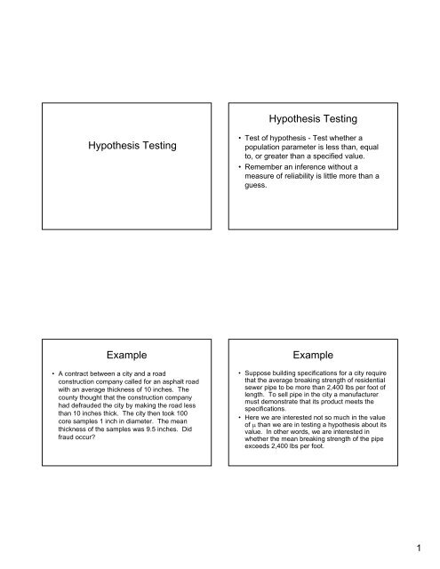
Hypothesis Testing<br />
Hypothesis Testing<br />
• Test of hypothesis - Test whether a<br />
population parameter is less than, equal<br />
to, or greater than a specified value.<br />
• Remember an inference without a<br />
measure of reliability is little more than a<br />
guess.<br />
Example<br />
• A contract between a city and a road<br />
construction company called for an asphalt road<br />
with an average thickness of 10 inches. The<br />
county thought that the construction company<br />
had defrauded the city by making the road less<br />
than 10 inches thick. The city then took 100<br />
core samples 1 inch in diameter. The mean<br />
thickness of the samples was 9.5 inches. Did<br />
fraud occur?<br />
Example<br />
• Suppose building specifications for a city require<br />
that the average breaking strength of residential<br />
sewer pipe to be more than 2,400 lbs per foot of<br />
length. To sell pipe in the city a manufacturer<br />
must demonstrate that its product meets the<br />
specifications.<br />
• Here we are interested not so much in the value<br />
of μ than we are in testing a hypothesis about its<br />
value. In other words, we are interested in<br />
whether the mean breaking strength of the pipe<br />
exceeds 2,400 lbs per foot.<br />
1
Hypotheses Statements<br />
• Two hypotheses:<br />
– Null hypothesis (H 0 ) - status quo to the party<br />
performing the experiment. The hypothesis will not<br />
be rejected unless the data provide convincing<br />
evidence that it is false.<br />
– Alternative or research hypothesis (H a ) - which will<br />
be accepted only if the data provide convincing<br />
evidence of its truth.<br />
Hypotheses Statements<br />
Examples<br />
• For pipe example:<br />
– (H0) μ ≤ 2 , 400 (the pipe does not meet<br />
specifications)<br />
– (Ha) μ > 2 , 4 0 0 (the pipe meets specifications)<br />
• How can the city decide when enough evidence<br />
exists to conclude the pipe meets specifications?<br />
– When the sample mean x convincingly indicates that<br />
the population mean exceeds 2,400 lbs per foot.<br />
Evidence<br />
• “Convincing” evidence in favor of the alternative<br />
exists when the value of x exceeds 2,400 by<br />
an amount that cannot be readily attributed to<br />
sampling variability.<br />
• We need to compute a “test statistic” which will<br />
be the z-value that measures the distance<br />
between the values of x and the value of<br />
μ specified in the null hypothesis.<br />
• The test statistic is:<br />
Example<br />
x − x 2 400<br />
z<br />
μ −<br />
= =<br />
,<br />
σ σ<br />
x<br />
n<br />
• A value of z=1 means that x-bar is 1<br />
standard deviation above μ = 2,<br />
400<br />
• A value of z=1.5 means that x-bar is 1.5<br />
standard deviations above μ = 2,<br />
400<br />
2
Two Types of Errors:<br />
Type I Error<br />
• Deciding that the null hypothesis is false when in<br />
fact it is true is called a Type I error. In the<br />
graph shown, the probability of making a Type I<br />
error is only:<br />
• =P(Type 1 error)<br />
α = 0 . 0 5<br />
• =P(reject H0 when in fact H0 is true)<br />
• =P(z > 1.645 when in fact<br />
μ = 2 , 4 0 0 )=0.05<br />
The Test Itself<br />
• Null and alternative hypothesis:<br />
H 0<br />
: μ = 2 , 4 0 0<br />
H a<br />
: μ > 2,<br />
400<br />
• Test statistic:<br />
x<br />
z =<br />
− 2,<br />
400<br />
• Rejection region:<br />
• z > 1 6 4 5 for<br />
.<br />
• Example: assume<br />
x = 2, 460 s = 200 n = 50<br />
• What is your decision?<br />
σ<br />
x<br />
. α = 0 0 5<br />
Two Types of Errors:<br />
Type II Error<br />
• Accepting the null hypothesis when in fact it is<br />
false is called a Type II error. We denote the<br />
probability of committing a Type II error by β .<br />
• Usually difficult to determine so we simply say<br />
that the sample evidence is insufficient to reject<br />
the null hypothesis at the α = 005 . confidence<br />
level.<br />
Decisions and Consequences<br />
for a Test of Hypothesis<br />
True State of Nature<br />
Decision Ho True Ha True<br />
Choose Ho Correct Decision Type II Error<br />
Choose Ha Type I Error Correct Decision<br />
A Type I error has a probability of α .<br />
A Type II error has a probability of β .<br />
3
Elements of a Test of<br />
Hypothesis<br />
• 1. Null Hypothesis<br />
• 2. Alternative Hypothesis<br />
• 3. Test Statistic<br />
• 4. Rejection Region<br />
• 5. Assumptions<br />
• 6. Sample and Calculate Test Statistic<br />
• 7. Conclusion<br />
Steps for Selecting the Null and<br />
Alternative Hypotheses<br />
1. Select the alternative hypothesis - 3 types:<br />
One-tailed, upper tail H a : μ > 2400<br />
One-tailed, lower tail H a : μ < 2400<br />
Two-tailed H a : μ ≠ 2400<br />
2. Select the null hypothesis as the status quo,<br />
which will be presumed true unless the<br />
sample evidence conclusively establishes the<br />
alternative hypothesis: H o : μ = 2400<br />
Large-Sample Test of Hypothesis<br />
about a Mean<br />
• Use the z-statistic.<br />
• Example - A farmer hypothesizes that the mean<br />
yield of soybeans per acre is greater than 520<br />
bushels. A sample of 36 1-acre plots results in<br />
a sample mean value of 543 with a standard<br />
deviation of 124. At a .025 level, can we<br />
conclude that the mean yield is above 520?<br />
Small-Sample Test of Hypothesis<br />
about a Mean<br />
• If n is small, we cannot assume that the sample<br />
standard deviation will provide a good<br />
approximation of the population standard<br />
deviation. We must use the t-distribution rather<br />
than the z-distribution to make inferences about<br />
the population mean.<br />
• Test Statistic:<br />
t<br />
=<br />
x − μ 0<br />
s<br />
n<br />
4
Example<br />
• A tire company guarantees that a particular tire<br />
has a mean useful lifetime of 42,000 miles or<br />
more. A consumer testing agency, wishing to<br />
verify this claim, observed n=10 tires on a test<br />
wheel that simulated normal road conditions.<br />
The lifetimes (in thousands of miles) were as<br />
follows: 42, 36, 46, 43, 41, 35, 43, 45, 40, 39.<br />
Use these data to determine whether there is<br />
sufficient evidence to contradict the<br />
manufacturers claim at the .05 level.<br />
P-Values<br />
• For all the hypothesis testing examples so far,<br />
the value of α and thus the rejection region are<br />
selected prior to conducting the test.<br />
• A second method is to report the extent to which<br />
the statistic disagrees with the null hypothesis<br />
and letting the reader decide whether to reject<br />
the null hypothesis. This measure of<br />
disagreement is called the p-value.<br />
Steps for Calculating the p-<br />
value<br />
• Choose the maximum level of a you are willing to<br />
tolerate.<br />
• Determine the value of the test statistic z from the<br />
sample data. Look up the z-statistic and find the<br />
corresponding probability:<br />
– One-tailed test - the p-value = tail area beyond z<br />
in the same direction as the alternative<br />
hypothesis.<br />
– Two-tailed test - the p-value= 2 times the tail area<br />
beyond the z value in the direction of the sign of<br />
z.<br />
• Reject the null hypothesis if the observed p-value is<br />
less than α.<br />
Example<br />
• According to a national survey, the price of a new family<br />
home averages $115,000. You hypothesize that the<br />
average price in your city exceeds the national average.<br />
To test your belief, you record the prices of 20 new<br />
homes in your city and find the sample mean to equal<br />
$120,000 with a sample standard deviation of $30,000.<br />
If α =.05, does the data support your belief? What is the<br />
p-value? What would be the result if the sample was<br />
100 homes with the same mean and standard deviation<br />
above? What is the p-value?<br />
5
Large Sample Test of Hypothesis about<br />
a Binomial Probability<br />
• Inferences about proportions (or percentages)<br />
are often made in the context of the probability,<br />
p, of “success” for a binomial distribution.<br />
• Previously we have calculated a confidence<br />
interval for p.<br />
• For hypothesis tests on proportions, do not use<br />
the sample proportion to calculate the standard<br />
deviation. Instead, use the standard deviation<br />
based on the value of the null hypothesis.<br />
•H 0 :<br />
•H a :<br />
p<br />
• Test statistic:<br />
• Rejection region:<br />
Hypothesis Test<br />
= p<br />
0<br />
p><br />
p0<br />
p<<br />
p0<br />
p≠<br />
p<br />
0<br />
p$<br />
− p<br />
z =<br />
σ<br />
z<br />
z<br />
z<br />
p$<br />
><br />
<<br />
0<br />
><br />
z<br />
z<br />
α<br />
α<br />
z<br />
α<br />
2<br />
• Where<br />
x<br />
$p =<br />
n<br />
p q<br />
σ $p =<br />
n<br />
0 0<br />
Example<br />
• A rating service for local radio stations claims<br />
that 40% of the prime drive-time audience listens<br />
to WXIX. You are the advertising manager of a<br />
competing radio station and you doubt that<br />
WXIX’s market share is that large. Formulate<br />
and test the appropriate hypothesis at the 5%<br />
significance level if 380 people out of 1,000<br />
surveyed say that they listen to WXIX. What is<br />
the p-value?<br />
6
The Relationship Between Confidence<br />
Intervals and Hypothesis Tests<br />
• A Confidence Interval is really a two-tailed<br />
Hypothesis Test (at the same α-level):<br />
– For a confidence interval, we are (1-α)% sure that the<br />
true value of the population statistic is between the<br />
lower confidence level (LCL) and the upper<br />
confidence level (UCL). We are α% sure that the true<br />
value of the population statistic is not in this range.<br />
– For a hypothesis test, we either (1) fail to reject H0 at<br />
the (1-α)% level effectively creating a confidence<br />
interval or (2) reject H0 in favor of Ha which is the<br />
area outside of the confidence interval.<br />
Example<br />
• Our previous farmer example:<br />
– A farmer hypothesizes that the mean yield of<br />
soybeans per acre is not equal to 520 bushels.<br />
Sampling info of 36 one-acre plots finds a sample<br />
mean of 543 with a standard deviation of 124.<br />
– At a 0.10 level, can we conclude that the mean yield<br />
is not equal to 520?<br />
– Construct a 90% confidence interval using the above<br />
information.<br />
Two Population Means, μ 1 and μ 2<br />
• Independent Samples:<br />
– Mean income of households in two different<br />
neighborhoods in Fairfax County, VA: Incomes in<br />
one neighborhood are unrelated (independent) to<br />
incomes in the other neighborhood.<br />
• Dependent Samples:<br />
– Mean daily sales of two restaurants located on the<br />
same block in New York City: Is there a difference in<br />
daily sales volume between the two restaurants?<br />
Independent Sampling<br />
• Consider the Sampling Distribution of ( X1 − X 2)<br />
– The Mean of the sampling distribution of<br />
( μ<br />
1<br />
− μ<br />
2<br />
) is ( X<br />
1<br />
− X<br />
2<br />
)<br />
– Since the two samples are independent, the<br />
standard deviation of the sampling distribution<br />
(standard error of ( X ) ) is:<br />
1<br />
− X<br />
2<br />
σ σ<br />
σ = +<br />
( X 1 − X 2 )<br />
n n<br />
– The sampling distribution of ( X is )<br />
1<br />
− X<br />
2<br />
approximately normal for large samples (Central<br />
Limit Theorem) so use a z-statistic.<br />
2<br />
1<br />
1<br />
2<br />
2<br />
2<br />
7
Large Sample Hypothesis Test for<br />
(μ 1 - μ 2 ) - Independent Sampling<br />
• One-tailed Test:<br />
– H 0 : (μ 1 - μ 2 ) = D 0 (or 0) vs Ha: (μ 1 - μ 2 ) > D 0 (or 0)<br />
– H 0 : (μ 1 - μ 2 ) = D 0 (or 0) vs Ha: (μ 1 - μ 2 ) < D 0 (or 0)<br />
• Two-tailed Test:<br />
– H 0 : (μ 1 - μ 2 ) = D 0 (or 0) vs Ha: (μ 1 - μ 2 ) not equal to D 0 (or 0)<br />
• Test statistic:<br />
( x1<br />
− x2<br />
) − D0<br />
zcalc<br />
=<br />
σ<br />
( x −x<br />
)<br />
σ σ<br />
σ = +<br />
( X 1 − X 2 )<br />
n n<br />
1<br />
2<br />
2<br />
1<br />
1<br />
2<br />
2<br />
2<br />
Small Sample Confidence Interval for<br />
(μ 1 - μ 2 ) - Independent Sampling<br />
• Both populations must be approximately<br />
normally distributed with equal variances (these<br />
variances are usually unknown):<br />
s<br />
2<br />
p<br />
x<br />
−<br />
(<br />
1 2 α ( x 1 − x 2 )<br />
2<br />
( x<br />
=<br />
1<br />
−<br />
x ) ± t<br />
x ) ± t<br />
2<br />
α<br />
2<br />
σ<br />
s<br />
2<br />
p<br />
⎛ 1<br />
⎜<br />
⎝ n<br />
2<br />
( n − 1 ) s + ( n − 1 )<br />
1<br />
n<br />
1<br />
1<br />
+<br />
n<br />
2<br />
−<br />
2<br />
1<br />
2<br />
=<br />
+<br />
1 ⎞<br />
⎟<br />
n<br />
2 ⎠<br />
s<br />
2<br />
2<br />
Small Sample Hypothesis Test for<br />
(μ 1 - μ 2 ) - Independent Sampling<br />
• One-tailed Test:<br />
– H 0 : (μ 1 - μ 2 ) = D 0 (or 0) vs Ha: (μ 1 - μ 2 ) > D 0 (or 0)<br />
– H 0 : (μ 1 - μ 2 ) = D 0 (or 0) vs Ha: (μ 1 - μ 2 ) < D 0 (or 0)<br />
• Two-tailed Test:<br />
– H 0 : (μ 1 - μ 2 ) = D 0 (or 0) vs Ha: (μ 1 - μ 2 ) not equal to D 0 (or 0)<br />
• Test statistic:<br />
( x − x ) − D<br />
t =<br />
s<br />
2<br />
p<br />
=<br />
1<br />
2<br />
⎛<br />
s<br />
p<br />
⎜<br />
⎝<br />
2<br />
1<br />
n<br />
1<br />
+<br />
1<br />
n<br />
2<br />
0<br />
⎞<br />
⎟<br />
⎠<br />
2<br />
( n −1) s + ( n − )<br />
1<br />
1 2<br />
1 s<br />
n + n − 2<br />
1<br />
2<br />
2<br />
2<br />
Dependent Sampling<br />
• We are unable to use the two-sample (μ 1 - μ 2 )<br />
method for performing hypothesis tests and<br />
calculating confidence intervals if the samples<br />
are dependent on some external factor.<br />
• Instead, use Paired Difference method which<br />
takes sample dependence into account when<br />
performing hypothesis tests and calculating<br />
confidence intervals.<br />
8
Paired Difference Method<br />
• The test statistic becomes:<br />
x<br />
D<br />
− 0<br />
t =<br />
⎛ ⎞<br />
⎜<br />
s<br />
D ⎟<br />
⎝ n<br />
D ⎠<br />
– Assumptions:<br />
• The distribution of differences is approximately normally<br />
distributed.<br />
• The sample differences are random.<br />
Paired Difference Hypothesis<br />
Test<br />
• One-tailed Test:<br />
– H0: (μ1 - μ2) = D0 (or 0) vs Ha: (μ1 - μ2) > D0 (or 0)<br />
μD = D0 (or 0) μD > D0 (or 0)<br />
– H0: (μ1 - μ2) = D0 (or 0) vs Ha: (μ1 - μ2) < D0 (or 0)<br />
μD = D0 (or 0) μD < D0 (or 0)<br />
• Two-tailed Test:<br />
– H0: (μ1 - μ2) = D0 (or 0) vs Ha: (μ1 - μ2) not equal to D0 (or 0)<br />
μD = D0 (or 0) μD not equal to D0 (or 0)<br />
• Test statistic:<br />
x<br />
=<br />
⎛<br />
⎜<br />
⎝<br />
− D<br />
s ⎞<br />
D ⎟<br />
n<br />
D ⎠<br />
D 0<br />
t<br />
where t has (n D -1)<br />
degrees of<br />
freedom<br />
9


