A Simple and Effective Spectral Feature for Speech Detection ... - OFAI

Proc. of the 15 th Int. Conference on Digital Audio Effects (DAFx-12), York, UK , September 17-21, 2012
A SIMPLE AND EFFECTIVE SPECTRAL FEATURE FOR SPEECH DETECTION IN
MIXED AUDIO SIGNALS
Reinhard Sonnleitner 1 , Bernhard Niedermayer 1
1 Department for Computational Perception
Johannes Kepler University of Linz
Gerhard Widmer 1,2 , Jan Schlüter 2
2 Austrian Research Institute for
Artificial Intelligence, Vienna
ABSTRACT
We present a simple and intuitive spectral feature for detecting
the presence of spoken speech in mixed (speech, music, arbitrary
sounds and noises) audio signals. The feature is based on some
simple observations about the appearance, in signals that contain
speech, of harmonics with characteristic trajectories. Experiments
with some 70 hours of radio broadcasts in five different languages
demonstrate that the feature is very effective in detecting and delineating
segments that contain speech, and that it also seems to be
quite general and robust w.r.t. different languages.
1. INTRODUCTION
Detecting speech in mixed audio signals is a task that humans can
easily accomplish even in noisy environments, or when they do
not understand a foreign language. The identification of those segments
in an audio stream that contain speech (as opposed to, or in
combination with, other sounds like music or arbitrary noises) is
a fundamental prerequisite for many speech processing tasks, e.g.,
automatic speech recognition, speaker diarisation and automatic
story segmentation [1]. In the domain of audio signal processing
the task of Voice Activity Detection (VAD) is well established.
However, most authors in that field (see [2], [3], or [4], for example)
focus on the detection of voice in noisy environments, or in
the presence of reverberation.
Less research has been conducted on identifying and delineating
segments containing spoken speech in complex mixed audio
signals such as arbitrary radio or TV broadcast streams. Especially
for radio and TV broadcasts, the determining factors vary
considerably from the more limited VAD scenario, and more varied
mixtures of sounds need to be considered. [5] compare hierarchical
and multi-class approaches to speech/music segmentation
via Support Vector Machines. Audio features for this task are automatically
selected from an initial set of about 600 features of various
types, using a feature selection method. Detection of singing
voice in music tracks is performed in [6], by extraction and selection
of partials depending on vibrato and tremolo parameters
that are characteristic for voice and discriminative with respect to
musical instruments.
Discrimination of speech from non-speech samples like environmental
sounds, animal vocalizations and music has been investigated,
e.g., in [7]. The authors used a data corpus consisting of
speech samples from an Acoustic-Phonetic corpus, and dedicated
non-speech samples, but not from complex mixed signals, as one
will often encounter in real-world data. They report near perfect
speech classification. However, the speech samples in their audio
database represent clean speech rather than complex mixtures.
Generalization to unseen data was tested by artificially distorting
the clean speech samples with noise and reverberation.
In the area of speech/music discrimination, [1] classify audio
segments to one of three categories: silence, music, and a category
consisting of two subcategories, speech and speech with music.
They report to extract 94 different features based on Linear
Prediction Cepstral Coefficients (LPCC), Mel Frequency Cepstral
Coefficients (MFCC), Line Spectral Pairs (LSP) and the Shorttime
Fourier Transform (STFT) on a data corpus that consists of
10 hours of Mandarin news broadcasts The data includes speech
from news speakers, interviews with different speakers, ambient
noises and different genres of music, but no vocal music with instrumental
accompaniment is included in the data. The ground
truth is determined by using supplied automatic speech recognition
transcripts for semi-automatic labeling of the aforementioned
four categories. Near perfect evaluation results with F-Measure
round 0.97 to 0.98 are reported for three different classifiers based
on the above-mentioned general sets of features.
[8] address the tasks of discriminating between speech, monophonic
singing, and polyphonic music. It is pointed out that the
discrimination between speech and monophonic singing demands
for more sophisticated algorithms than the task of discriminating
speech from polyphonic music. The experiments are based on a
data corpus that consists of 1000 samples of speech, 1114 samples
of singing performed by 58 persons and 200 samples of polyphonic
music. Prior to signal type discrimination, the continuous audio
stream is segmented into short clips based on changes in intensity.
Starting from a set of 276 audio features, automatic feature selection
methods are applied. For the best classifier (an ensemble classifier
based on a reduced feature set computed on the segments), a
final error rate of 0.57% is reported.
In this paper, we propose a single novel spectral feature for
identifying the presence of speech in arbitrary mixed audio signals.
We present a straightforward machine learning classifier based on
this feature, and show – in experiments with an extensive and diverse
corpus of real-world radio broadcasts – that the feature works
surprisingly well, even across different languages. The advantages
of the new feature are its extreme simplicity (it amounts to 1 number
per audio frame), its intuitive comprehensibility and, related to
that, the fact that the feature (or classifiers based on it) can be easily
tuned to the specific requirements of a given application problem
(e.g., to balance recall against precision).
2. A SIMPLE FEATURE FOR SPEECH DETECTION
In the following, we define a single spectral feature to detect spoken
speech on the basis of a logarithmically scaled representation
of the STFT. The feature is motivated by some simple observations
concerning spectro-temporal variations of speech signals.
DAFX-1

Proc. of the 15 th Int. Conference on Digital Audio Effects (DAFx-12), York, UK , September 17-21, 2012
2.1. Observations on Speech Signals
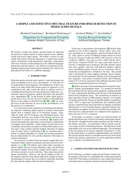
When comparing the spectrogram of a speech signal to signals representing
music or noise, one will observe a number of specific
characteristics.
• First, speech signals usually display patterns relating to the
presence of several harmonics, that are influenced by the
shape of the vocal tract. Within an individual time frame,
they manifest themselves in the form of significant peaks
within the spectrum. This behavior is similar to the sound
produced by (pitched) musical instruments. There, partials
can be found at the fundamental frequency f 0 of a tone and
also near its integer multiples (n + 1)f 0, with n ∈ N or
n ∈ N e for string or wind instruments, respectively.
• A second important observation is that the harmonics are
sustained over a certain span of time in which they are very
likely to vary in frequency. This is a discriminative characteristic
of speech in comparison to noise or the sound of
musical instruments. Noise, on the one hand, does generally
not reveal significant spectral peaks which are sustained
over time. Musical instruments, on the other hand,
are used to play tones on a discrete pitch scale. A corresponding
audio signal will, therefore, consist of partials
with a relatively constant frequency. 1 Exceptions to this
are specific effects like glissandi and – a somewhat more
serious problem for speech/music discrimination – vibrato.
(We will return to this issue in Section 4 below.)
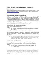
In Figure 1, one can clearly recognize the characteristic curved
trajectories in the spectrogram computed from the speech signal.
In contrast, the music sample is characterized by strictly horizontal
and minor vertical structures in the lower frequency regions, i.e.,
the partials at the harmonic frequencies of notes and the respective
transient note onsets. The third sample shows the frequency
components present in traffic noise. Here, one cannot identify any
dominant pattern.
Based upon those observations, we propose to identify human
voice within mixed audio signals by detecting the curved frequency
trajectory of the harmonics over a certain period of time.
2.2. Feature Computation
The basic idea behind the feature we propose is to capture sustained
harmonics’ trajectories which – in contrast to the partials of
a note played on a musical instrument – vary in frequency. Both
phenomena result in a high correlation when comparing the spectral
patterns of two nearby audio frames. Therefore, each time
frame X t is compared to a subsequent one X t+offset . However, in
order to allow for the curved frequency trajectories of speech harmonics,
frequency shifts have to be accounted for. We do this by
computing the cross-correlation between the two time frames X t
and X t+offset . The cross-correlation can be used to estimate the
degree of correlation between shifted versions of these vectors, for
a range of so-called lags l. Given two vectors x and y of length
N, the cross-correlation for all lags l ∈ [−N, N] including zerolag,
as given in Equation 1, results in a cross-correlation series of
length 2N + 1.
R xy(l) = ∑ x iy i+l (1)
i
1 In [9], this is exploited in a feature called Continuous Frequency Activation
(CFA) for (foreground and background) music detection in TV
broadcasts.
In our case the input vectors are time frames, and the lag corresponds
to a shift along the frequency axis. We define r xcorr as the
maximum cross-correlation over a range of lags:
r xcorr (X t, X t+offset ) = max R Xt ,X t+offset
(l) (2)
l
where l ∈ [−l max, l max] denotes the lag (frequency shift) in
terms of frequency bins. We define r as a special case of the crosscorrelation
mentioned above, with lag l = 0 , and subsequently
refer to zero-lag cross-correlation as correlation:
r(X t, X t+offset ) = R Xt ,X t+offset
(0) (3)
As an indicator of the dominance of speech in an audio signal,
we introduce the correlation gain r xcorr − r. For ‘ideal’ musiconly
signals (i.e, those dominated by horizontal tone patterns in
the spectrum), the cross-correlation will have its maximum for
frequency lag 0, and thus the gain r xcorr − r = R(0) − r =
r − r = 0. For signals dominated by curved harmonic patterns,
R(l) will be maximal for some l ≠ 0 and there will be a positive
gain r xcorr − r. For audio recordings where musical instruments
dominate the contribution of speech to the signal the gain
is lowered. Here, harmonics of varying frequency are mixed with
partials of constant frequency. For sections containing noise only,
the correlation between nearby time frames is generally expected
to be low. Also, it is unlikely that a frequency shift will yield significantly
higher correlations due to the randomness of the energy
distribution over time in such signals.
Since harmonic frequencies are multiples of the fundamental
frequency, shifting spectral patterns along the frequency axis
cannot be done on a linear scale: the lag parameter in the crosscorrelation
formula can only represent the frequency derivative
∆f of one single harmonic; for the other harmonics this derivative
would be a multiple c k ∆f. However, when frequencies are represented
on a logarithmic scale, harmonics are at constant offsets
relative to their fundamental frequency, so continuous frequency
changes can be captured by cross-correlation as described above.
We prepare our data corpus for subsequent computations by
sampling the input to 22.05 kHz monaural audio. To extract the
spectral feature, we transform the audio input to the frequency domain
by applying a Short Time Fourier Transform with a Kaiser
window of a size of 4096 samples. For subsequent computations
in the feature extraction process, we follow the preprocessing steps
as performed in [9], by computing the magnitude spectrum |X(f)|
and mapping the STFT magnitude spectrum to a perceptual scale.
For our implementation we have chosen the logarithmic cent scale
representation of STFT spectrograms. Also, the feature extraction
process considers the lower 150 cent-scaled frequency bins of the
spectrum only, which corresponds to frequencies of up to roughly
802 Hz, while discarding the upper bins.
Using this configuration we found that comparing an audio
frame to its direct successor does not yield the expected results.
The hop size chosen for the STFT corresponds to a time difference
of approximately 23 ms. During such a small time span the
harmonics’ frequencies do not vary significantly enough to permit
a reliable discrimination from partials of notes played by musical
instruments. Therefore, the parameter offset in the computation
of the cross-correlation (cf. Equation 2) was chosen to be 3.
Another parameter that has to be selected is the maximum lag
l max used for computing the cross-correlation (cf. Equation 2).
We propose to set this parameter such that it does not allow for the
shift of an entire semitone, which in our case gives us an l max of
DAFX-2

Proc. of the 15 th Int. Conference on Digital Audio Effects (DAFx-12), York, UK , September 17-21, 2012
(a) Speech (b) Music (c) Traffic Noise
Figure 1: Comparison of the spectrograms of sections containing (a) speech, (b) popular music including singing voice, and (c) traffic
noise. The length of each section is approximately 7 seconds and the frequencies range from 100 Hz to 3000 Hz on a logarithmic scale.
3. This prevents the feature from reporting high values at times
where a musical instrument plays along a chromatic scale.
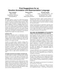
Figure 2 demonstrates the behavior of our feature. We show
intermediate results of the feature computation process, for two
different exemplary kinds of audio input: a transition from speech
to music is shown in the left half of the figure, a Pop song with
female sung voice is depicted on the right. Once again, note that
the cross-correlation value for lag l = 0 corresponds to the ‘regular’
correlation. Thus, in the plots in the second row of Fig. 2,
which show the cross-correlation values for different lags l (vertical
dimension, in the range of l ∈ [−3, 3]), high values in the
central row (l = 0) indicate high correlation, whereas high values
for rows with l ≠ 0 are possible indicators of speech. The former
can clearly be seen in the music examples (first half of plot on
left-hand side, and entire plot on right-hand side). The latter case
can be observed in the second half of the plot on the left, where
the presence of curved harmonic patterns in the spectrogram leads
to relatively high cross-correlation values for lags l < 0 – higher,
at any rate, than the correlation at lag l = 0. The resulting correlation
gain r xcorr − r, shown at the bottom of the figure, then
identifies exactly those areas that exhibit strong curved patterns.
(The somewhat spiky nature of the gain function also explains why
we will apply some smoothing to this curve when computing the
actual features for the classifier – see below).
2.3. The Final Feature: Context Integration and Smoothing
We compute the feature from the audio signal according to a decision
frequency of 5 Hz (i.e., one feature value every 200 ms),
where we center an observation window of width 50 STFT blocks
(approximately 1.3s) around each decision position, in order to
also capture some context.
For each of the N−offset pairs of STFT blocks (X t, X t+offset )
in the observation window of length N, two vectors xc, c of feature
values, one for the cross-correlation and one for the correlation
results, are computed, both having a length of N − offset,
where N is the number of STFT blocks of the observation window
(50, in our case). The element-wise difference of the vectors
gives the feature vector r = xc − c. Finally, r is smoothed using
a rectangular window of width 5, and the index of the dominant
frequency bin within the observation window is appended to the
feature vector as an additional feature. Preliminary experiments
showed that this increases the ratio of correctly classified instances
by roughly one percentage point. Thus, the final result is a vector
of 48 feature values (50 − 3 smoothed correlation gain values, and
1 frequency bin index) per decision point. The size of the observation
window allows us to capture enough context to detect spoken
speech, and carries overlap for effective smoothing that can be applied
as a post-processing step.
3.1. Classification Scenario
3. EXPERIMENTAL RESULTS
We test our feature in a classical machine learning approach, by
training a classifier on a manually annotated ground truth (radio
broadcast recordings with segment boundary indications) for a basic
two-class problem, namely for the classes contains speech and
does not contain speech. The used classifier model is a random
forest [10] (an ensemble classifier of decision trees that outputs
the mode of the decisions of its respective trees), parameterized to
use 200 decision trees, and 10 random features per tree. The classifier
outputs class probabilities, which are transformed to binary
decisions using simple thresholding.
We prepare three data sets: a training set, to be used as training
material for the classifier; a validation set, which will be used
to perform systematic parameter studies, and to select the final parameter
setting (in particular, the decision threshold); and an independent
test set, on which the final classifier will then be evaluated.
The classifier is trained to classify individual time points in the
audio stream — in other words, each training example is one point
in the audio, represented in terms of a feature vector of 48 feature
values, as explained above, where the feature values characterize
the signal at the current point, and its local context.
Training, validation, and test data are processed with a feature
extraction frequency of 5 Hz, which means that the classifier
produces predictions at a rate of 5 labels per second of audio. As
a post-processing step, the sequence of predicted class labels is
smoothed using a median filter with a window size of 52 labels.
3.2. The Data Corpus
The main data corpus consists of recordings of 61 hours of randomly
selected radio broadcasts, recorded in three batches (each
relating to a different week) from six different radio stations in
DAFX-3

Proc. of the 15 th Int. Conference on Digital Audio Effects (DAFx-12), York, UK , September 17-21, 2012
150
FM4−h1.wav; lower 150 cent bins;4.8065s at second1209
150
FM4−h3.wav; lower 150 cent bins;4.8065s at second854
100
100
50
50
20 40 60 80 100 120 140 160 180 200
20 40 60 80 100 120 140 160 180 200
Cross−correlation, offset=3, maxlag=3
Cross−correlation, offset=3, maxlag=3
2
2
0
0
−2
−2
20 40 60 80 100 120 140 160 180
20 40 60 80 100 120 140 160 180
0.01
vector of max(result) over each column
xcorr
corr
0.01
vector of max(result) over each column
xcorr
corr
0.005
0.005
0
0 20 40 60 80 100 120 140 160 180 200
0
0 20 40 60 80 100 120 140 160 180 200
x Result: (xcorr − corr), smoothed
10−4
8
6
4
2
0
0 20 40 60 80 100 120 140 160 180 200
(a) Music-Speech transition
x Result: (xcorr − corr), smoothed
10−4
8
6
4
2
0
0 20 40 60 80 100 120 140 160 180 200
(b) Music and sung voice
Figure 2: Comparison of the feature values for sections containing (a) music and then spoken speech and (b) music with singing voice
(duration: approximately 5 seconds each). The top row shows the spectrograms (the lower 150 bins of the cent scale) of the two audio
snippets. The second row shows the resulting cross-correlation values R(l) for offset = 3 and lag values l ∈ [−3, 3]. The third row
compares the corresponding values r(= R(0)) (dashed line) and r xcorr = max l R(l) (solid line). The bottom row plots the correlation
gain r xcorr − r, which is the basis for our proposed feature.
Switzerland (drsvirus, RSI Rete 2, RSR Couleur 3, Radio Central,
Radio Chablais, RTR Rumantsch), which together represent all
four official languages of Switzerland: (Swiss) German, French,
Italian and Rumantsch. The recordings were split into files with a
duration of 30 minutes each, and manually annotated according to
the two-class problem of ‘spoken speech’ vs. ‘other’, where ‘spoken
speech’ refers to all segments which contain speech, even if
mixed with other sounds or music (such as when a radio host introduces
a song while it is already playing). 2 Note that this classi-
2 Of course, the distinction between speech and non-speech is not always
entirely clear, and neither are the exact boundaries where a speech
signal ends or begins. (As as simple example, consider pauses in between
sentences. In a sense, these are a natural part of the way we speak; but if
such pauses grow longer, at some (rather arbitrary) point we will have to
classify them as non-speech.) This observation, in fact, makes us slightly
skeptical of some of the results in the literature, where recognition accuracies
in speech/non-speech segmentation of 100% or almost 100% are
reported. Our own preliminary experiments with multiple annotators per
fication problem is considerably more difficult that distinguishing
pure speech samples from pure music or noise samples.
The training set consists of 21 hours of audio (42 half hour
files, 7 files from each radio station) randomly selected from the
first two Swiss week batches. The validation set comprises 18 half
hour files (3 per station). The random forest classifier is trained on
the manually annotated ground truth; thresholds as well as postprocessing
parameters are chosen empirically using the validation
set.
The audio files for the independent test set were recorded two
weeks after training and validation data. The test set is made up
of 31 hours of previously unseen broadcast material, split into 62
files, distributed almost uniformly over the 6 radio stations.
Finally, to further test the robustness of the feature in relation
to different languages and dialects, we recorded an additional 9
audio file indicate an inter-annotator variability of up to 2%. Thus, not
even the so-called ground truth is 100% reliable (nor can it be).
DAFX-4

Proc. of the 15 th Int. Conference on Digital Audio Effects (DAFx-12), York, UK , September 17-21, 2012
1.0
1.0
0.9
1.0
0.8
0.8
0.8
0.7
0.8
Accuracy
0.6
0.4
Recall
0.6
0.4
0.6
0.5
0.4
0.3
F-Score
0.6
0.4
0.2
0.2
0.2
0.2
0.1
0.0
0.0 0.2 0.4 0.6 0.8 1.0
threshold
0.0
0.0 0.2 0.4 0.6 0.8 1.0
Precision
0.0
0.0
0.0 0.2 0.4 0.6 0.8 1.0
threshold
(a) Accuracy
(b) Precision / Recall
(c) F-score
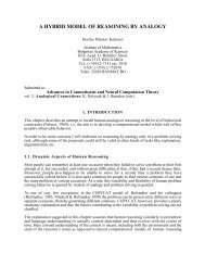
Figure 3: Accuracy, Precision vs. Recall and F-measure plots for thresholds t ∈ [0.0, 1.0], showing the robustness of the spoken speech
feature. In plot (b), the thresholds are indicated by colors.
hours of radio material from Switzerland’s neighbor country Austria
(3 stations: Oe1, Oe3, LiveRadio). The class distributions and
segment counts for the various data sets are given in Table 2.
are generally rather high and testify to the power of our simple
audio feature. Clearly, though, there is still some room for further
improvement, which we will address in future research.
3.3. Results
Figure 3 shows how the results on the validation set change as we
vary the decision threshold for the classifier. (Remember that the
classifier outputs a probability value between 0 and 1 for a given
example, which is then turned into a binary class prediction by
thresholding.) The classifier turns out to be extraordinarily stable
for a wide range of decision thresholds between 0.2 and 0.8. As
a consequence, we rather arbitrarily selected a threshold of 0.5 for
our remaining evaluation on independent test sets.
The results of the resulting classifier on the validation and test
sets are summarised and compared in Table 1. Given the complexity
of the signals and the task (which we are keenly aware of, having
annotated some of the audio files ourselves), F-Score values
over 0.93 must be considered extremely good – especially considering
that the classification is essentially based on 1 feature only.
Note again that we could easily direct the classifier towards other
points on the recall/precision trade-off continuum by changing the
decision threshold.
In order to assess the robustness and generality of the feature in
relation to different languages, we also performed specialized classification
experiments. Specifically, we trained five special classifiers,
one for each of the languages French, Italian, Rumantsch,
Swiss-German and Austrian German. The training sets for each
of these specialized classifiers consisted of 9 hours of broadcast
data (see Table 2). We did not need any validation sets for these
experiments, as we simply kept the threshold and post-processing
filter parameters that we used with the main classifier (a threshold
of 0.5 and a median filter over 52 samples).
The results of these experiments are shown in Table 3. While
there are some interesting deviations for certain pairs of languages
(in particular one that lends itself to a joke between Swiss and
Austrians, namely the particularly low mutual performance of the
classifiers related to Austrian and Swiss German – both of which
are supposed to be variants of a common language 3 ), the results
3 This is in stark contrast to the group of Romanic languages (French,
Italian, Rumantsch), whose relatedness shows very clearly in the classification
results.
4. DISCUSSION
We have proposed a simple, efficiently computable spectral feature
for precisely detecting spoken speech within complex, mixed
audio streams, as encountered in real world broadcast media content.
The feature’s dimensionality is 1, as one value per STFT
block is computed. The classifier is presented a several blockswide
observation window of feature values, which results, in our
configuration, in a feature vector of length 48, as explained in Section
2.3. In practice, feature values tend to be rather small numbers,
often in the range of 0 to 10 −3 . The feature values could be
transformed into the interval [0.0, 1.0] by representing the result
as: 1.0 − r/r xcorr for every result with correlation gain, and zero
otherwise.
Our feature has several advantages. It is extremely simple,
with a clear and intuitive interpretation. It is easily computable
– also in real time –, which also makes it a candidate for on-line
speech detection tasks. Generally, classifiers based on a single
feature are easy to understand and control.
One topic that we only hinted at in Section 2.1 above and did
not discuss in the rest of the paper is the ‘problem’ of vibrato
in singing, and in certain instruments. It is to be expected that
our ‘curved shape detection feature’ will also produce a positive
cross-correlation gain in passages containing a clear vibrato – and
indeed, focused tests with opera recordings show that it does. The
fact that this did not seem to be a big problem in the experiments
reported in this paper may be due to the fact that there was rather
little classical music contained in our audio material. On the other
hand, it seems that the problem of discriminating speech from sung
vibrato issue should be relatively easy to solve, as vibrato passages
in singing or instrument playing tend to be much longer than spoken
vowels – a musically meaningful vibrato needs a sustained
tone of considerable length. We are currently carrying out some
specialized investigations into this issue.
DAFX-5

Proc. of the 15 th Int. Conference on Digital Audio Effects (DAFx-12), York, UK , September 17-21, 2012
Dataset thresh. TP [s] FP [s] True ratio [%] Est. ratio [%] Acc.[%] Prec.[%] Recall [%] F-Score [%]
Validation Set 0.5 10664.8 456.6 35.06 34.33 96.44 95.89 93.88 94.87
Test Set 0.5 30041.4 1122.2 29.81 27.87 96.06 96.40 90.14 93.16
Table 1: Classification performance: Averaged true and false positives and quality measurements. TP/FP = true/false positives; “ratio” =
“percentage of speech segments in relation to total duration of recording”.
Dataset #files speech[s] speech[%] #speech other [s] #other Audio[s] #Sgmts
Train Set 42 22215.4 28.7 572 55117.5 595 77332.8 1167
Validation Set 18 11360.5 35.0 203 21039.3 208 32399.8 411
Test Set 62 33327.3 29.8 995 78471.5 1023 111799 2018
Dataset #files speech[s] speech[%] #speech other [s] #other Audio[s] #Sgmts
Austrian 18 11298.2 34.9 545 21102.4 549 32400.6 1094
French 18 11184.8 34.7 216 21030.1 221 32214.9 437
Italian 18 14446.6 44.5 176 18004.8 178 32451.4 354
Rumantsch 18 7236.87 22.3 249 25216.2 260 32453 509
Swiss German 18 4486.57 13.8 202 27963.4 217 32450 419
Table 2: Distribution of segment lengths and segment counts within the data corpus, by datasets and by languages. “#speech” means
“number of continuous segments labeled as containing speech (possibly mixed with other sounds)”.
Austrian Classifier TP [s] FP [s] True ratio [%] Est. ratio [%] Acc.[%] Prec.[%] Recall [%] F-Score [%]
French 10817.2 436.0 34.72 34.93 97.50 96.13 96.70 96.41
Italian 13828.8 234.0 44.51 43.33 97.38 98.34 95.73 97.01
Rumantsch 6999.6 434.6 22.30 22.91 97.93 94.15 96.73 95.42
Swiss German 3729.4 1096.6 13.83 14.87 94.29 77.28 83.13 80.10
French Classifier TP [s] FP [s] True ratio [%] Est. ratio [%] Acc.[%] Prec.[%] Recall [%] F-Score [%]
Austrian 9486.2 570.0 35.04 31.04 92.47 94.33 83.54 88.61
Italian 12298.0 100.2 44.51 38.20 93.07 99.19 85.13 91.63
Rumantsch 6789.8 212.2 22.30 21.58 97.97 96.97 93.83 95.37
Swiss German 3644.4 461.8 13.83 12.65 95.98 88.75 81.23 84.83
Italian Classifier TP [s] FP [s] True ratio [%] Est. ratio [%] Acc.[%] Prec.[%] Recall [%] F-Score [%]
Austrian 10686.2 1090.8 35.04 36.35 94.57 90.74 94.11 92.39
French 10940.4 1169.4 34.72 37.59 95.61 90.34 97.81 93.93
Rumantsch 7097.2 644.2 22.30 23.85 97.59 91.68 98.08 94.7
Swiss German 3976.4 2668.8 13.83 20.48 90.20 59.84 88.63 71.44
Rumantsch Cl. TP [s] FP [s] True ratio [%] Est. ratio [%] Acc.[%] Prec.[%] Recall [%] F-Score [%]
Austrian 10138.6 1195.4 35.04 34.98 92.56 89.45 89.29 89.37
French 10916.2 1067.6 34.72 37.20 95.85 91.09 97.59 94.23
Italian 12718.4 127.4 44.51 39.58 94.28 99.01 88.04 93.20
Swiss German 3962.6 2105.0 13.83 18.70 91.90 65.31 88.32 75.09
Swiss Classifier TP [s] FP [s] True ratio [%] Est. ratio [%] Acc.[%] Prec.[%] Recall [%] F-Score [%]
Austrian 8084.6 470.4 35.04 26.40 88.45 94.50 71.20 81.21
French 10129.2 179.0 34.72 32.00 96.16 98.26 90.55 94.25
Italian 11354.0 87.0 44.51 35.26 90.20 99.24 78.60 87.72
Rumantsch 6517.6 159.2 22.30 20.57 97.29 97.62 90.07 93.69
Table 3: Averaged true and false positives and quality measurements for classifiers trained on different languages
DAFX-6

Proc. of the 15 th Int. Conference on Digital Audio Effects (DAFx-12), York, UK , September 17-21, 2012
Acknowledgements
This research was funded by the Austrian Science Fund FWF under
projects L511 and Z159.
[13] B. Schuller, G. Rigoll, and K. Lang M. “Discrimination of
speech and monophonic singing in continuous audio streams
applying multi-layer support vector machines,” in International
Conference on Multimedia Computing and Systems,
2004, pp. 1655–1658.
5. REFERENCES
[1] C. Liu, L. Xie, and H. Meng, “Classification of music
and speech in mandarin news broadcasts,” in 9 th National
Conference on Man-Machine Speech Communication
(NCMMSC), Huangshan, Anhui, China, Oct. 21-24, 2007.
[2] K. Metha, C. K. Pham, and E. S. Chng, “Linear dynamic
models for voice activity detection,” in Proceedings 12 th
Annual Conf. Int. Speech Communication Association, Florence,
Italy, Aug. 27-31, 2011.
[3] J. Pohjalainen, T. Raitio, and P. Alku, “Detection of shouted
speech in the presence of ambient noise,” in Proceedings
12 th Annual Conf. Int. Speech Communication Association,
Florence, Italy, 2011.
[4] T. Petsatodis, F. Talantzis, C. Boukis, Z. Tan, and R. Prasad,
“Multi-sensor voice activity detection based on multiple observation
hypothesis testing,” in Proceedings of the 12 th
Annual Conf. Int. Speech Communication Association, Florence,
Italy, 2011.
[5] M. Ramona and G. Richard, “Comparison of different strategies
for a svm-based audio segmentation,” in European Signal
Processing Conference (EUSIPCO), Glasgow, UK, Sept.
2009.
[6] L. Regnier and G. Peeters, “Singing voice detection in music
tracks using direct voice vibrato detection,” IEEE International
Conference on Acoustics, Speech, and Signal Processing,
vol. 0, pp. 1685–1688, 2009.
[7] N. Mesgarani, M. Slaney, and S. Shamma, “Discrimination
of speech from nonspeech based on multiscale spectrotemporal
modulations,” in IEEE Transactions on Audio,
Speech and Language Processing, 2006, pp. 920–930.
[8] B. Schuller, B. Schmitt B. J. D. Arsic, S. Reiter, K. Lang M.
and G. Rigoll, “Feature selection and stacking for robust discrimination
of speech, monophonic singing, and polyphonic
music,” in IEEE International Conference on Multimedia &
Expo, 2005, pp. 840–843.
[9] K. Seyerlehner, T. Pohle, M. Schedl, and G. Widmer, “Automatic
music detection in television productions,” in Proceedings
of the Int. Conf. on Digital Audio Effects, Bordeaux,
France, 2007.
[10] Leo Breiman, “Random forests,” Machine Learning, vol. 45,
no. 1, pp. 5–32, 2001.
[11] J. Bach, J. Anemueller, and B Kollmeier, “Robust speech detection
in real acoustic backgrounds with perceptually motivated
features,” Speech Communication, vol. 53, no. 5, pp.
690–706, 2011.
[12] N. Mesgarani, S. Shamma, and M. Slaney, “Speech discrimination
based on multiscale spectro-temporal modulations,”
IEEE International Conference on Acoustics Speech and Signal
Processing, vol. 1, no. 3, pp. 601–604, 2004.
DAFX-7