Convergent Decomposition Solvers for Tree-reweighted Free ... - OFAI
Convergent Decomposition Solvers for Tree-reweighted Free ... - OFAI
Convergent Decomposition Solvers for Tree-reweighted Free ... - OFAI

You also want an ePaper? Increase the reach of your titles
YUMPU automatically turns print PDFs into web optimized ePapers that Google loves.
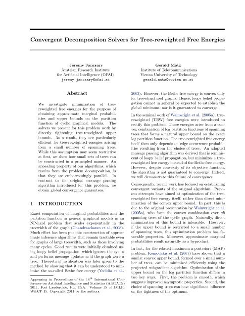
<strong>Convergent</strong> <strong>Decomposition</strong> <strong>Solvers</strong> <strong>for</strong> <strong>Tree</strong>-<strong>reweighted</strong> <strong>Free</strong> Energies<br />
Jeremy Jancsary<br />
Austrian Research Institute<br />
<strong>for</strong> Artificial Intelligence (<strong>OFAI</strong>)<br />
jeremy.jancsary@ofai.at<br />
Gerald Matz<br />
Institute of Telecommunications<br />
Vienna University of Technology<br />
gerald.matz@tuwien.ac.at<br />
Abstract<br />
We investigate minimization of tree<strong>reweighted</strong><br />
free energies <strong>for</strong> the purpose of<br />
obtaining approximate marginal probabilities<br />
and upper bounds on the partition<br />
function of cyclic graphical models. The<br />
solvers we present <strong>for</strong> this problem work by<br />
directly tightening tree-<strong>reweighted</strong> upper<br />
bounds. As a result, they are particularly<br />
efficient <strong>for</strong> tree-<strong>reweighted</strong> energies arising<br />
from a small number of spanning trees.<br />
While this assumption may seem restrictive<br />
at first, we show how small sets of trees can<br />
be constructed in a principled manner. An<br />
appealing property of our algorithms, which<br />
results from the problem decomposition, is<br />
that they are embarrassingly parallel. In<br />
contrast to the original message passing<br />
algorithm introduced <strong>for</strong> this problem, we<br />
obtain global convergence guarantees.<br />
1 INTRODUCTION<br />
Exact computation of marginal probabilities and the<br />
partition function in general graphical models is an<br />
NP-hard problem that scales exponentially in the<br />
treewidth of the graph (Chandrasekaran et al., 2008).<br />
Much ef<strong>for</strong>t has been put into construction of approximate<br />
inference algorithms that remain tractable even<br />
<strong>for</strong> graphs of large treewidth, such as those involving<br />
many cycles. Good results were initially obtained using<br />
loopy belief propagation, which ignores the cycles<br />
and per<strong>for</strong>ms message updates as if the graph were a<br />
tree. Theoretical justification was later given to the<br />
method by showing that it can be understood to minimize<br />
the so-called Bethe free energy (Yedidia et al.,<br />
Appearing in Proceedings of the 14 th International Conference<br />
on Artificial Intelligence and Statistics (AISTATS)<br />
2011, Fort Lauderdale, FL, USA. Volume 15 of JMLR:<br />
W&CP 15. Copyright 2011 by the authors.<br />
2003). However, the Bethe free energy is convex only<br />
<strong>for</strong> tree-structured graphs. Hence, loopy belief propagation<br />
cannot in general be expected to establish the<br />
global minimum, nor is it guaranteed to converge.<br />
In the seminal work of Wainwright et al. (2005a), tree<strong>reweighted</strong><br />
(TRW) free energies were introduced to<br />
rectify this problem. These energies arise from a convex<br />
combination of log partition functions of spanning<br />
trees that <strong>for</strong>ms a natural upper bound on the exact<br />
log partition function. The tree-<strong>reweighted</strong> free energy<br />
itself then only depends on edge occurrence probabilities<br />
resulting from the choice of trees. An adapted<br />
message passing algorithm was derived that is reminiscent<br />
of loopy belief propagation, but minimizes a tree<strong>reweighted</strong><br />
free energy instead of the Bethe free energy.<br />
However, despite convexity of its objective function,<br />
the algorithm is not guaranteed to converge. Indeed,<br />
we will demonstrate this failure of convergence.<br />
Consequently, recent work has focused on establishing<br />
convergent variants of the original algorithm. Previous<br />
attempts have aimed at optimization of the tree<strong>reweighted</strong><br />
free energy itself, rather than direct minimization<br />
of the convex upper bound. In part, this is<br />
due to the original presentation by Wainwright et al.<br />
(2005a), who <strong>for</strong>m the convex combination over all<br />
spanning trees of the cyclic graph. Naturally, direct<br />
minimization of this bound is infeasible. However,<br />
if the upper bound is restricted to a small number<br />
of spanning trees, this optimization problem has favorable<br />
properties. Moreover, approximate marginal<br />
probabilities result naturally as a byproduct.<br />
In fact, <strong>for</strong> the related maximum-a-posteriori (MAP)<br />
problem, Komodakis et al. (2007) have shown that a<br />
similar convex upper bound, <strong>for</strong>med over a small number<br />
of trees, can be minimized efficiently using the<br />
projected subgradient algorithm. Optimization of the<br />
upper bound on the log partition function differs in<br />
two key ways. First, the problem is smooth, which<br />
suggests improved asymptotic properties. Second, the<br />
choice of spanning trees can have significant influence<br />
on the tightness of the optimum.
<strong>Convergent</strong> <strong>Decomposition</strong> <strong>Solvers</strong> <strong>for</strong> <strong>Tree</strong>-<strong>reweighted</strong> <strong>Free</strong> Energies<br />
In this paper, we make the following contributions:<br />
(a) We investigate direct minimization of tree<strong>reweighted</strong><br />
upper bounds on the log partition function<br />
using the spectral projected gradient algorithm (Birgin<br />
et al., 2000) and the projected quasi-Newton algorithm<br />
(Schmidt et al., 2009). The core of the resulting algorithms<br />
is embarrassingly parallel and we demonstrate<br />
that it scales accordingly in the number of processors.<br />
(b) We present strategies <strong>for</strong> choosing small sets of<br />
spanning trees and study their effect on the error of<br />
marginal probabilities, tightness of the upper bound<br />
and computational cost. These results are of general<br />
interest as the choice of trees (or edge probabilities) is<br />
mandated by any tree-<strong>reweighted</strong> algorithm.<br />
2 BACKGROUND<br />
Next, we briefly review the most important concepts<br />
we will be concerned with.<br />
2.1 UNDIRECTED GRAPHICAL MODELS<br />
We consider undirected graphical models G with vertex<br />
set V and edge set E defined over n discrete random<br />
variables with pairwise interactions. The probability<br />
of a particular variable state x ∈ X n thus factors as<br />
⎛<br />
⎞<br />
p(x; θ) = exp θ s (x s ) +<br />
∑<br />
θ st (x st ) − Φ(θ) ⎠ ,<br />
⎝ ∑ s∈V<br />
(s,t)∈E<br />
where the log partition function is defined as<br />
⎛<br />
⎞<br />
Φ(θ) = log ∑ ⎝ ∑ θ s (x s ) + ∑ θ st (x st ) ⎠ .<br />
s<br />
(s,t)<br />
x∈X n exp<br />
We shall find it convenient to express the same factorization<br />
using a vector-valued indicator function φ(x),<br />
which maps a variable state to binary indicators <strong>for</strong><br />
the corresponding components of θ ∈ R d :<br />
and similarly,<br />
p(x; θ) = exp (φ(x) · θ − Φ(θ)) , (1)<br />
Φ(θ) = log ∑<br />
x∈X n exp (φ(x) · θ) . (2)<br />
Subsequently, we will be concerned with computation<br />
of approximations to Φ(θ) and the marginal probabilities<br />
E{φ α (x)} = ∑<br />
x∈X n p(x; θ)φ α (x), (3)<br />
where we use α to refer to a single index corresponding<br />
to a particular state of a vertex s or an edge (s, t).<br />
Interestingly, the first and second derivatives of Φ(θ)<br />
generate the cumulants<br />
∂Φ(θ)<br />
∂θ α<br />
= E{φ α (x)} and ∂2 Φ(θ)<br />
∂θ α ∂θ β<br />
= cov{φ α (x), φ β (x)}.<br />
Hence, the marginal probabilities are given precisely<br />
by the gradient of the log partition function. Moreover,<br />
the covariance matrix, which is by definition positive<br />
semi-definite, <strong>for</strong>ms the Hessian. Convexity of the<br />
log partition function follows from this property.<br />
2.2 TREE-REWEIGHTED BOUNDS<br />
Consider now the set T = {T } of all spanning trees<br />
of a cyclic graph G. We use I(T ) to denote the set of<br />
indices {α} corresponding to states x s of vertices and<br />
x st of edges that belong to a particular tree T . Each of<br />
the spanning trees is associated with a parameterization<br />
θ(T ) that is tractable by the structural assumption.<br />
Wainwright et al. (2005a) observe that a convex<br />
combination ∑ T<br />
ρ(T )Φ(θ(T )) over trees yields an upper<br />
bound on Φ(θ) if the tractable parameter vector<br />
⃗θ = [θ(T 1 ), . . . , θ(T m )] ∈ R md lies in the convex set<br />
{<br />
}<br />
θ<br />
C(θ) = ⃗θ<br />
α (T ) = 0 <strong>for</strong> all T, α /∈ I(T )<br />
∣ ∑<br />
T ρ(T )θ(T ) = θ , (4)<br />
and ρ = {ρ(T )} is constrained to belong to the simplex<br />
of distributions over T ,<br />
∆ =<br />
{ρ ∣ ∑ }<br />
T ρ(T ) = 1, ρ(T ) ≥ 0 . (5)<br />
Observe that ρ must also be valid in the sense that<br />
each edge is covered with non-zero probability, otherwise<br />
C(θ) is empty. The upper bound property now<br />
follows directly from Jensen’s inequality:<br />
Φ(θ) = Φ (∑ T ρ(T )θ(T )) ≤ ∑ T<br />
ρ(T )Φ(θ(T )).<br />
The structural constraints θ α (T ) = 0 in C(θ) are not<br />
required <strong>for</strong> the upper bound to hold, but we include<br />
them in our presentation to make explicit the fact that<br />
the parameterizations θ(T ) are tractable.<br />
A natural question is then how to obtain the tightest<br />
upper bound possible within this framework. For a<br />
given distribution ρ over spanning trees, and target<br />
parameters θ, we can simply optimize over the set of<br />
tractable parameterizations θ, ⃗<br />
∑<br />
ρ(T )Φ(θ(T )). (6)<br />
min<br />
⃗θ∈C(θ)<br />
T<br />
Since the upper bound is a convex combination of convex<br />
functions, and the constraint set is convex, this is<br />
a convex optimization problem.
Jeremy Jancsary, Gerald Matz<br />
2.3 TREE-REWEIGHTED ENERGIES<br />
By <strong>for</strong>ming the Lagrangian of (6) and exploiting the<br />
conjugate duality relation between the log partition<br />
function and the negative entropy of a distribution,<br />
one can obtain an equivalent dual problem:<br />
max<br />
µ∈L(G)<br />
{<br />
µ · θ + ∑ s H(µ s) − ∑ (s,t) ν stI(µ st )<br />
}<br />
, (7)<br />
where µ s and µ st have interpretations as node and<br />
edge pseudomarginals, H(·) and I(·) denote the Shannon<br />
entropy and the mutual in<strong>for</strong>mation, respectively,<br />
and the constraint set<br />
{<br />
L(G) = µ ≥ 0<br />
∣<br />
∑<br />
x s<br />
µ s (x s ) = 1<br />
∑<br />
x st∼x s<br />
µ st (x st ) = µ s (x s )<br />
}<br />
(8)<br />
ensures proper local normalization and marginalization<br />
consistency 1 . The edge probabilities ν = {ν st }<br />
are strictly positive and arise from the valid distribution<br />
ρ ∈ ∆ over spanning trees.<br />
The objective function in (7) is the negative tree<strong>reweighted</strong><br />
free energy. As the dual of a convex function,<br />
it is concave in µ, and strong duality holds. The<br />
primary advantage of problem (7) over (6) is its reduced<br />
dimensionality: it is independent of the number<br />
of spanning trees involved. However, constraint set<br />
L(G) is considerably more complicated than C(θ).<br />
3 APPROACH<br />
The original message passing algorithm by Wainwright<br />
et al. (2005a) can be understood to per<strong>for</strong>m block coordinate<br />
updates in the Lagrangian of (7). However,<br />
without further precautions, the scheme is not guaranteed<br />
to converge. In practice, “damping” strategies are<br />
often applied to improve the convergence characteristics.<br />
In contrast, we investigate efficient methods <strong>for</strong><br />
direct minimization of (6). The coupling constraints<br />
in C(θ) are more easy to handle than L(G), and convergent<br />
minimization schemes thus arise naturally. We<br />
next discuss several key aspects of our approach.<br />
3.1 OBTAINING MARGINALS<br />
An approximation to the log partition function is naturally<br />
given by the optimum of problem (6). In contrast,<br />
it is not so obvious how to obtain approximate<br />
marginals from the solution. The key observation here<br />
arises en route of deriving (7) from (6): By <strong>for</strong>ming the<br />
Lagrangian of (6), and taking derivatives with respect<br />
to θ α , one obtains the stationary conditions<br />
E θ ⋆ (T ){φ α (x)} ! = µ α <strong>for</strong> all T, α ∈ I(T ) .<br />
1 We use x st ∼ x s to denote edge states x st that are<br />
consistent with node state x s.<br />
Consequently, at the optimal solution ⃗ θ ⋆ , all trees<br />
share a single set of marginals. To construct a full set<br />
of pseudomarginals µ, <strong>for</strong> each index α, we can thus<br />
use the marginal probability of any tree T <strong>for</strong> which<br />
α ∈ I(T ) once (6) is solved to optimality. Notably,<br />
the marginals of any tree can be obtained efficiently.<br />
3.2 COMPUTING THE GRADIENT<br />
As we pointed out in section 2.1, the derivative of the<br />
log partition function Φ(·) with respect to θ α is given<br />
by the corresponding marginal probability, E{φ α (x)}.<br />
Given that (6) is a weighted sum of such partition<br />
functions, it is easy to see that the full gradient<br />
∇ ⃗θ = ∑ [<br />
0 · · · ρ(T )Eθ(T ) {φ(x)} · · · 0 ]<br />
T<br />
= [ ρ(T 1 )E θ(T1){φ(x)}, . . . , ρ(T m )E ]<br />
θ(Tm){φ(x)}<br />
is thus given as a vector of weighted component gradients.<br />
In principle, this gradient can be computed<br />
very efficiently; the only concern is the number m of<br />
spanning trees involved. We discuss this issue in great<br />
detail in section 3.5.<br />
3.3 HANDLING THE CONSTRAINTS<br />
We now turn to discussion of the constraint set<br />
C(θ),<br />
∑<br />
defined in (4). Both the coupling constraints<br />
T<br />
ρ(T )θ(T ) = θ and the structural constraints<br />
θ α (T ) = 0 are linear, so C(θ) defines a convex polytope.<br />
As we shall point out, projection onto this set<br />
can be realized very efficiently. Formally, we search<br />
the solution to the following optimization problem:<br />
P θ ( θ ⃗ ∥<br />
′ ) = argmin∥⃗ θ − ⃗ ∥ θ<br />
′ 2 . (9)<br />
2<br />
⃗θ∈C(θ)<br />
For all T , if α /∈ I(T ), the structural constraints<br />
prescribe θ α (T ) = 0. These components are hence<br />
fully<br />
∑<br />
specified. Otherwise, the coupling constraints<br />
T ρ(T )θ α(T ) = θ α must be satisfied. Among the admissible<br />
{θ α (T )} <strong>for</strong> a given index α, whose weighted<br />
sum must be θ α , the sum of squares is minimized if<br />
(θ α (T )−θ α(T ′ )) 2 is equal <strong>for</strong> all trees T with α ∈ I(T ).<br />
Consider now the distance from the target parameter<br />
δ α = ( ∑ T ρ(T )θ′ α(T )−θ α ) and the accumulated probability<br />
mass σ α = ∑ T :α∈I(T )<br />
ρ(T ). It can be verified<br />
that the projection given by<br />
{<br />
P θ ( θ ⃗′ θ α (T ) = 0 if α /∈ I(T )<br />
) =<br />
θ α (T ) = θ α(T ′ (10)<br />
) − δα<br />
σ α<br />
otherwise<br />
ensures satisfaction of all constraints while adhering<br />
to the optimality criterion discussed above. Hence, it<br />
provides a solution to (9) which can be computed in<br />
O(md), i.e. in time linear in the dimensionality of ⃗ θ.
<strong>Convergent</strong> <strong>Decomposition</strong> <strong>Solvers</strong> <strong>for</strong> <strong>Tree</strong>-<strong>reweighted</strong> <strong>Free</strong> Energies<br />
Algorithm 1: TightenBound<br />
(SPG Variant)<br />
input : set of trees T and valid distribution ρ, target<br />
parameters θ, arbitrary initial θ ⃗(1) , step size<br />
interval [α min, α max], history length h<br />
output: pseudomarginals µ, upper bound ˜Φ ≥ Φ(θ)<br />
⃗θ (1) ← P θ ( θ ⃗(1) )<br />
˜Φ (1) ← parallelized ∑ T ρ(T )Φ(θ(1) (T ))<br />
α (1) ← 1/‖P θ ( θ ⃗(1) − ∇ (1)<br />
⃗θ<br />
) − θ ⃗(1) ‖<br />
k ← 1<br />
while ‖P θ ( θ ⃗(k) − ∇ (k)<br />
⃗θ<br />
d (k) ← P θ ( θ ⃗(k) − α (k) ∇ (k)<br />
⃗θ<br />
repeat<br />
) − ⃗ θ (k) ‖ < ε do<br />
) − ⃗ θ (k)<br />
choose λ ∈ (0, 1) ; e.g. via interpolation<br />
⃗θ (k+1) ← θ ⃗(k) + λd (k)<br />
˜Φ (k+1) ← parallelized ∑ T ρ(T )Φ(θ(k+1) (T ))<br />
until ˜Φ(k+1) < max{ ˜Φ (k) , . . . , ˜Φ (k−h) } + ɛλ∇ (k) · d<br />
⃗θ<br />
s (k) ← θ ⃗(k+1) − θ ⃗(k)<br />
y (k) ← ∇ (k+1) − ∇ (k)<br />
⃗θ<br />
⃗θ<br />
α (k+1) ← min{α max, max{α min, (s (k)·s (k) )/(s (k)·y (k) )}}<br />
k ← k + 1<br />
return ( ˜Φ (k) , marginals{∇ (k) }) ; see section 3.1<br />
⃗θ<br />
3.4 TIGHTENING THE BOUND<br />
For now, assume that ρ(T ) > 0 <strong>for</strong> a small number of<br />
trees T only. The gradient of our objective in (6) can<br />
then be computed efficiently. Moreover, the constraint<br />
set C(θ) is convex and can be projected onto at little<br />
cost. A principal method <strong>for</strong> optimization in such a<br />
setting is the projected gradient algorithm. However,<br />
this basic method can be improved on.<br />
3.4.1 Spectral Projected Gradient Method<br />
The main improvements of the spectral projected gradient<br />
(SPG) method (Birgin et al., 2000) over classic<br />
projected gradient descent are a particular choice of<br />
the step size (Barzilai and Borwein, 1988) and a nonmonotone,<br />
yet convergent line search (Grippo et al.,<br />
1986). In the setting of unconstrained quadratics, the<br />
SPG algorithm has been observed to converge superlinearly<br />
towards the optimum. We outline its application<br />
to (6) in Algorithm 1. Besides the mandatory<br />
input T , ρ and θ, the meta parameters [α min , α max ]<br />
specify the interval of admissible step sizes, and history<br />
length h specifies how many steps may be taken without<br />
sufficient decrease of the objective. If the number<br />
of steps is exceeded, backtracking is per<strong>for</strong>med<br />
and the step size is decremented until sufficient decrease<br />
has been established. In our implementation,<br />
we chose α min = 10 −10 , α max = 10 10 and h = 10. In<br />
the backtracking step, we simply multiply with a factor<br />
λ = 0.3. In practice, we found Algorithm 1 to be very<br />
robust with respect to the choice of meta parameters.<br />
(a)<br />
(b)<br />
Figure 1: (a) Two “snakes” cover any grid; (b) Two more<br />
mirrored replicas achieve symmetric edge probabilities.<br />
Proposition 1. For a given set of spanning trees T ,<br />
valid distribution over trees ρ and target parameters θ,<br />
Algorithm 1 converges to the global optimum of (6).<br />
Proof (Sketch). Convergence follows from the analysis<br />
of the SPG method by Wang et al. (2005).<br />
3.4.2 Projected Quasi-Newton Method<br />
The projected quasi-Newton (PQN) method was recently<br />
introduced by Schmidt et al. (2009) and can<br />
be considered a generalization of L-BFGS (Nocedal,<br />
1980) to constrained optimization. At each iteration,<br />
a feasible direction is found by minimizing a quadratic<br />
model subject to the original constraints:<br />
min ˜Φ (k) +( θ− ⃗ θ ⃗(k) )·∇ (k)<br />
⃗θ + 1 2 (⃗ θ−θ ⃗(k) ) T B (k) ( θ− ⃗ θ ⃗(k) )<br />
⃗θ∈C(θ)<br />
where B (k) is a positive-definitive approximation to<br />
the Hessian that is maintained in compact <strong>for</strong>m in<br />
terms of the previous p iterates and gradients (Byrd<br />
et al., 1994). The SPG algorithm can be used to<br />
per<strong>for</strong>m the above minimization effectively. We hypothesized<br />
that PQN might compensate <strong>for</strong> the larger<br />
per-iteration cost through improved asymptotic convergence<br />
and thus implemented a scheme similar to<br />
Algorithm 1. We do not give a complete specification<br />
here, as it only differs from Algorithm 1 in the choice<br />
of the direction and the use of a traditional line search.<br />
3.5 CHOOSING THE SET OF TREES<br />
It is clear that Algorithm 1 is only efficient <strong>for</strong> a reasonably<br />
small number of selected trees with ρ(T ) > 0.<br />
We refer to this set as S and denote the corresponding<br />
vector of non-zero coefficients by ρ s . Subsequently, we<br />
discuss how to obtain S and ρ s in a principled manner.<br />
3.5.1 Uni<strong>for</strong>m Edge Probabilities<br />
According to the Laplacian principle of insufficient<br />
reasoning, one might choose uni<strong>for</strong>m edge occurrence<br />
probabilities given by ν st = (|V| − 1)/|E|. However,<br />
in our <strong>for</strong>mulation, we need to find a pair (S, ρ s ) that<br />
results in these probabilities. The dual coupling between<br />
(S, ρ s ) and ν is defined in terms of the map-
Jeremy Jancsary, Gerald Matz<br />
Algorithm 2: Covering<strong>Tree</strong>s<br />
input : graph G, stopping criterion<br />
output: selected trees S, valid ρ s<br />
S (1) ← {random spanning tree}, ρ (1)<br />
s ← [1], k ← 1<br />
while not criterion do<br />
ν (k) ← ν(S (k) , ρ s (k) ) ; compute edge probabilities<br />
S (k+1) ← S (k) ∪ MST(G, ν (k) ) ; MST f. edge cost ν (k)<br />
ρ (k+1)<br />
s ← 1/(k + 1) ; <strong>for</strong> 1 ∈ R k+1<br />
k ← k + 1<br />
return (S (k) , ρ s (k) )<br />
ping ν(S, ρ s ) = ∑ T ∈S ρ s(T )ν(T ), where ν(T ) ∈ R |E|<br />
indicates the edges contained in T , such that ν st (T ) =<br />
[(s, t) ∈ E T ]. Algorithm 2 establishes a suitable pair<br />
(S, ρ s ) in a greedy manner. At each step, we add a<br />
minimum spanning tree (MST) <strong>for</strong> weights given by<br />
the current edge probabilities. We stop when ν(S, ρ s )<br />
is sufficiently uni<strong>for</strong>m, which allows to trade off the<br />
number of resulting trees against uni<strong>for</strong>mity.<br />
Proposition 2. Algorithm 2 determines a sequence<br />
{ν(S (k) , ρ (k)<br />
s )} that converges to a vector u with components<br />
given by u st = (|V| − 1)/|E| as k → ∞.<br />
We outline a proof in the supplementary material, appendix<br />
A.1.1; Algorithm 2 takes conditional gradient<br />
steps that seek to minimize ‖ν(S, ρ s ) − u‖ 2 2.<br />
3.5.2 Snake-Based Strategy<br />
For grid-structured graphs, we also found that fairly<br />
uni<strong>for</strong>m edge occurrence probabilities could be obtained<br />
using four “snake”-shaped trees that in sum<br />
cover all edges. This is best seen in terms of an illustration,<br />
which we provide in Figure 1. If we choose<br />
ρ s = 1/|S|, the edges in the interior assume ν st = 1/2,<br />
whereas those on the boundary are given by ν st = 3/4.<br />
3.5.3 Constructing an Almost Minimal Set<br />
If we choose a different stopping criterion, namely<br />
ν st > 0 ∀(s, t), Algorithm 2 can also be used to greedily<br />
establish a set of trees that is almost minimal in<br />
the sense that its cardinality is close to the minimum<br />
number of spanning trees required to cover all edges<br />
of G. Note that there is no guarantee of optimality in<br />
this respect. However, in practice, we found that Algorithm<br />
2 was very effective at establishing such sets.<br />
3.5.4 Obtaining an Optimal Set<br />
Wainwright et al. (2005a) show that one can obtain<br />
even tighter upper bounds by optimizing (7) over the<br />
edge occurrence probabilities ν. This is achieved using<br />
conditional gradient steps, where each such outer<br />
Algorithm 3: Optimal<strong>Tree</strong>s<br />
input : graph G, target parameters θ<br />
output: selected trees S, valid ρ s, µ, ˜Φ ≥ Φ(θ)<br />
(S (l) , ρ (l)<br />
s ) ← Covering<strong>Tree</strong>s(G, ν st > 0 ∀(s, t))<br />
k ← l<br />
while not converged do<br />
( ˜Φ (k) , µ (k) ) ← TightenBound(S (k) , ρ (k)<br />
s , θ)<br />
i (k) ← [−I(µ (k)<br />
st ), −I(µ (k)<br />
uv ), . . .] ; negative MI per edge<br />
S (k+1) ← S (k) ∪ MST(G, i (k) ) ; MST f. edge cost i (k)<br />
ρ (k+1)<br />
s ← 1/(k + 1) ; <strong>for</strong> 1 ∈ R k+1<br />
k ← k + 1<br />
return (S (k) , ρ (k) ,TightenBound(S (k) , ρ (k)<br />
s , θ))<br />
iteration involves solution of (7) <strong>for</strong> the current iterate<br />
ν (k) and a subsequent minimum spanning tree<br />
(MST) search with edge weights given by the negative<br />
mutual in<strong>for</strong>mation (MI) of the current edge pseudomarginals,<br />
denoted by I(µ st ). The resulting bound<br />
is jointly optimal over ν and µ. Algorithm 3 defines<br />
a similar procedure <strong>for</strong> the primal space we are operating<br />
in. It successively establishes pairs (S, ρ s ) resulting<br />
in increasingly tighter upper bounds ˜Φ. The<br />
invocation of Covering<strong>Tree</strong>s(·) in the initialization<br />
phase ensures that we start from a valid distribution<br />
ρ s and a small set S such that each edge is covered<br />
with non-zero probability and Algorithm 1 can be applied.<br />
In practice, the biggest gains are achieved in the<br />
first few iterations. Hence, although it is expensive to<br />
find a suitable tree at each iteration, the number of<br />
trees stays relatively small, and we approach the joint<br />
optimum in the process.<br />
Proposition 3. Algorithm 3 determines a sequence<br />
{ ˜Φ (k) } converging to an upper bound ˜Φ ⋆ ≥ Φ(θ) that is<br />
jointly optimal over the choice of trees S, the distribution<br />
over trees ρ s , and the tractable parameterization<br />
⃗θ, as k → ∞.<br />
The sketch of a proof is given in appendix A.1.2.<br />
3.6 PARALLELIZING COMPUTATION<br />
The computational cost of Algorithm 1 is dominated<br />
by computation of ∑ T ρ(T )Φ(θ(k+1) (T )), which requires<br />
sum-product belief propagation on each tree<br />
T ∈ S. One might then assume that compared to<br />
traditional message passing algorithms, Algorithm 1<br />
incurs an overhead that is asymptotically linear in the<br />
number of selected trees. However, observe that the<br />
terms {Φ(θ (k+1) (T ))} are completely independent of<br />
each other. Hence, as long as the number of CPU cores<br />
is greater than or equal to the number of trees, we can<br />
avoid the additional cost by scheduling each run of belief<br />
propagation on a different core. As we shall see in<br />
section 4.2.3, this works very well in practice.
<strong>Convergent</strong> <strong>Decomposition</strong> <strong>Solvers</strong> <strong>for</strong> <strong>Tree</strong>-<strong>reweighted</strong> <strong>Free</strong> Energies<br />
Table 1: Impact of the set of spanning trees on the approximation error<br />
Grid IsingGauss Grid IsingUni<strong>for</strong>m Regular IsingGauss Complete ExpGauss<br />
e( ˜Φ) e(µ) e( ˜Φ) e(µ) e( ˜Φ) e(µ) e( ˜Φ) e(µ)<br />
4Snakes 0.085 ± 0.01 0.112 ± 0.01 0.104 ± 0.01 0.087 ± 0.00 ∼ ∼<br />
Minimal 0.088 ± 0.01 0.113 ± 0.01 0.109 ± 0.01 0.090 ± 0.00 0.833 ± 0.10 0.308 ± 0.05 0.397 ± 0.07 0.074 ± 0.01<br />
Uni<strong>for</strong>m 0.084 ± 0.01 0.110 ± 0.01 0.102 ± 0.01 0.085 ± 0.00 0.833 ± 0.10 0.308 ± 0.05 0.394 ± 0.07 0.074 ± 0.01<br />
⋆ Uni<strong>for</strong>m 0.083 ± 0.01 0.110 ± 0.01 0.101 ± 0.01 0.085 ± 0.00 0.833 ± 0.10 0.308 ± 0.05 0.394 ± 0.07 0.074 ± 0.01<br />
Optimal 0.031 ± 0.01 0.091 ± 0.02 0.053 ± 0.01 0.079 ± 0.01 0.832 ± 0.10 0.308 ± 0.05 0.377 ± 0.07 0.075 ± 0.01<br />
4 EXPERIMENTS<br />
We wanted to assess several aspects of our algorithms<br />
empirically. Towards this end, we considered four<br />
types of random graphs that varied with respect to<br />
their structure and the exponential parameters θ. 2<br />
Grid IsingGauss: an n g × n g grid of binary variables<br />
(X = {−1, +1}), with potentials chosen as<br />
θ s (x s ) = θx s and θ st (x st ) = θx s x t , where θ ∼ N (0, 1)<br />
was drawn independently <strong>for</strong> each node and edge.<br />
Grid IsingUni<strong>for</strong>m: Equal to the above, except that<br />
θ was drawn from U(−1, +1).<br />
Regular IsingGauss: A random regular graph with<br />
n r binary variables, each of which was connected to n d<br />
others, and potentials akin to Grid IsingGauss.<br />
Complete ExpGauss: A complete graph with n c<br />
variables (X = {0, 1, 2, 3}) and potentials independently<br />
drawn as θ s (x s ) = 0 and θ st (x st ) ∼ N (0, 1).<br />
4.1 IMPACT OF TREE SELECTION<br />
We considered four different ways of decomposing the<br />
cyclic graphs into spanning trees: 4Snakes, described<br />
in section 3.5.2; Minimal, described in section 3.5.3;<br />
Uni<strong>for</strong>m described in section 3.5.1; and finally Optimal<br />
(section 3.5.4). For the Uni<strong>for</strong>m decomposition,<br />
we stopped once min (s,t) ν st ≥ 0.9 max (s,t) ν st . The<br />
4Snakes decomposition was only applicable to grids.<br />
First, we wanted to assess the impact of the decomposition<br />
scheme on the approximation errors e( ˜Φ) =<br />
| ˜Φ − Φ(θ)|/Φ(θ) and e(µ) = ‖µ − E{φ(x)}‖ 1 /d. We<br />
generated 30 instances of each type of graph considered<br />
(with n g = 15, n r = 30, n d = 10 and n c = 10)<br />
and solved the corresponding instance of (6) to a tolerance<br />
of ε = 10 −5 using Algorithm 1. For the Optimal<br />
scheme, we used 50 outer iterations. The gains<br />
were minuscule beyond this point. The reference values<br />
Φ(θ) and E{φ(x)} were computed using join trees<br />
or brute <strong>for</strong>ce, depending on the type of graph.<br />
Table 1 shows the average and the standard deviation<br />
(indicated using ±) of the error over the 30 instances<br />
2 We used libDAI (Mooij, 2010) to generate instances.<br />
Table 2: Standard deviation of the approximation error<br />
<strong>for</strong> 30 runs over the same graphs and potentials, using<br />
different Minimal sets of trees at each run.<br />
e( ˜Φ) e(µ)<br />
Grid IsingGauss 0.096 ± 0.0018 0.113 ± 0.0012<br />
Grid IsingUni<strong>for</strong>m 0.112 ± 0.0019 0.090 ± 0.0010<br />
Regular IsingGauss 0.866 ± 0.0003 0.351 ± 0.0002<br />
Complete ExpGauss 0.355 ± 0.0023 0.076 ± 0.0004<br />
of each type of graph. The tree decomposition was<br />
computed anew <strong>for</strong> each instance. Unsurprisingly, the<br />
Optimal scheme per<strong>for</strong>med best almost universally,<br />
with large gains in some instances. More interestingly,<br />
the other three schemes were rather closely tied, with<br />
only a slight edge <strong>for</strong> the Uni<strong>for</strong>m decomposition.<br />
For comparison, we also computed the approximation<br />
errors resulting from analytically determined uni<strong>for</strong>m<br />
edge probabilities ( ⋆ Uni<strong>for</strong>m), which corresponds to<br />
an infinite number of iterations of Algorithm 2; the<br />
gains over the Uni<strong>for</strong>m scheme are negligible. Finally,<br />
we checked how deterministically the Minimal<br />
scheme behaved on a single given graph (considering<br />
its random nature). Table 2 shows that the deviation<br />
over 30 independent decompositions was very low.<br />
4.2 EFFECTIVENESS OF SOLVERS<br />
In a second series of experiments, we compared our<br />
own solvers (TrwSPG, outlined by Algorithm 1, and<br />
TrwPQN with p = 4) to the message passing algorithm<br />
(TrwMP) of Wainwright et al. (2005a) and<br />
a variant thereof (TrwDMP) that employs “damping”<br />
(α = 0.5). In our implementation of the latter,<br />
we updated the messages by iterating over the edges<br />
uni<strong>for</strong>mly at random. For comparison, we used the<br />
same types of graphs as in section 4.1, with n g = 50,<br />
n r = 100, n d = 10 and n c = 50.<br />
4.2.1 Asymptotic Efficiency<br />
First, we compared the asymptotic behavior of the<br />
competing solvers. To this end, we ran them on the<br />
same randomly generated instances of each type of<br />
graph. Figure 2 shows the progress of the objective<br />
as a function of iterations of the respective algorithm.<br />
The plot displays only a single run of each solver
Jeremy Jancsary, Gerald Matz<br />
˜Φ<br />
5,200<br />
4,950<br />
TrwSPG<br />
TrwPQN<br />
TrwMP<br />
TrwDMP<br />
˜Φ<br />
3,360<br />
3,260<br />
˜Φ<br />
1,980<br />
1,960<br />
˜Φ<br />
2,000<br />
1,500<br />
4,700<br />
0 10 20 30 40<br />
3,160<br />
0 10 20 30 40<br />
1,940<br />
0 10 20 30 40<br />
1,000<br />
0 20 40 60 80 100 120 140<br />
iteration<br />
iteration<br />
iteration<br />
iteration<br />
(a) Grid IsingGauss, Minimal<br />
(b) Grid IsingUni<strong>for</strong>m, Minimal<br />
(c) Reg. IsingGauss, Minimal<br />
(d) Comp. ExpGauss, Minimal<br />
Figure 2: Asymptotic efficiency—only a single run is depicted to highlight convergence characteristics.<br />
˜Φ<br />
5,200<br />
4,950<br />
TrwSPG<br />
TrwPQN<br />
TrwMP<br />
TrwDMP<br />
˜Φ<br />
3,360<br />
3,260<br />
˜Φ<br />
1,980<br />
1,960<br />
˜Φ<br />
2,000<br />
1,500<br />
4,700<br />
0 0.5 1 1.5<br />
3,160<br />
0 0.2 0.4 0.6 0.8 1<br />
1,940<br />
0 0.1 0.2 0.3<br />
1,000<br />
0 0.5 1 1.5 2<br />
running time (s)<br />
running time (s)<br />
running time (s)<br />
running time (s)<br />
(a) Grid IsingGauss, Minimal<br />
(b) Grid IsingUni<strong>for</strong>m, Minimal<br />
(c) Reg. IsingGauss, Minimal<br />
(d) Comp. ExpGauss, Minimal<br />
˜Φ<br />
5,200<br />
4,950<br />
TrwSPG<br />
TrwPQN<br />
TrwMP<br />
TrwDMP<br />
˜Φ<br />
3,330<br />
3,230<br />
˜Φ<br />
1,980<br />
1,960<br />
˜Φ<br />
2,000<br />
1,500<br />
4,700<br />
0 2 4 6 8<br />
3,130<br />
0 1 2 3 4 5 6<br />
1,940<br />
0 0.1 0.2 0.3 0.4<br />
1,000<br />
0 2 4 6 8 10 12<br />
running time (s)<br />
running time (s)<br />
running time (s)<br />
running time (s)<br />
(e) Grid IsingGauss, Uni<strong>for</strong>m<br />
(f) Grid IsingUni<strong>for</strong>m, Uni<strong>for</strong>m<br />
(g) Reg. IsingGauss, Uni<strong>for</strong>m<br />
(h) Comp. ExpGauss, Uni<strong>for</strong>m<br />
Figure 3: Computational efficiency of competing solvers—average over 10 runs is shown here.<br />
(rather than an average over multiple runs), so as not<br />
to “average out” the convergence characteristics. Due<br />
to a lack of space, we only show the curves <strong>for</strong> a particular<br />
set of trees obtained using the Minimal scheme;<br />
the others triggered similar asymptotic behavior.<br />
As one can see from Figure 2, the message updates<br />
per<strong>for</strong>med by TrwMP decrease the objective very<br />
rapidly. However, this comes at a price. In some<br />
cases, e.g. panel (c), the process diverges. We also<br />
note that the iterates produced by TrwMP need not<br />
lie within L(G). Feasibility is only guaranteed <strong>for</strong> the<br />
optimal solution; hence, the curve can fluctuate about<br />
the optimum, see panel (d). This can even happen<br />
<strong>for</strong> TrwDMP, which generally improves smoothness<br />
of convergence considerably, but decreases the objective<br />
more slowly. In contrast, the iterates of TrwSPG<br />
and TrwPQN are always guaranteed to yield an upper<br />
bound. In terms of smoothness of convergence,<br />
TrwPQN exposes the most desirable behavior. On<br />
the other hand, TrwSPG implements a compromise<br />
between smoothness and rapid decrease; while its nonmonotone<br />
line search can yield sporadic “bumps”, it<br />
ultimately converges to the global optimum.<br />
4.2.2 Computational Efficiency<br />
Next, we assessed the solvers in terms of their computational<br />
efficiency. For this purpose, we measured<br />
the progress of the objective as a function of running<br />
time, rather than iterations. We averaged the curve<br />
of each solver over 10 runs in order to smoothen any<br />
effects caused by the random nature of the updates<br />
per<strong>for</strong>med by TrwMP, or scheduling of the multiple<br />
CPU threads used by TrwSPG and TrwPQN. All<br />
results were obtained on a machine with eight Intel<br />
Xeon CPU cores running at 2.4 GHz.<br />
Figure 3 shows the resulting plots. We employed two<br />
decomposition schemes at opposing ends of the spectrum,<br />
Minimal (top row), and Uni<strong>for</strong>m (bottom<br />
row). As expected, the results varied significantly with<br />
the number of trees in use. For Minimal sets, we<br />
found that TrwSPG approached the optimum even<br />
more quickly than TrwMP, and much more so than<br />
TrwDMP. TrwPQN was also competitive in some<br />
cases, but was generally dominated by TrwSPG due<br />
to the lower per-iteration cost. On the other hand,<br />
TrwMP and its damped variant were more efficient<br />
<strong>for</strong> the larger Uni<strong>for</strong>m sets, since they only depend<br />
on the edge occurrence probabilities. This is particularly<br />
apparent in panels (e) and (f); over 50 spanning<br />
trees were required to achieve uni<strong>for</strong>m edge probabilities,<br />
which significantly outnumbered the available<br />
CPU cores. However, in section 4.1, we found that<br />
there is only limited gain in establishing Uni<strong>for</strong>m<br />
sets. Hence, one should definitely opt <strong>for</strong> a Minimal<br />
or 4Snakes strategy with TrwSPG and TrwPQN.<br />
In this regime, TrwSPG outper<strong>for</strong>med both TrwMP<br />
and TrwDMP while guaranteeing convergence.
<strong>Convergent</strong> <strong>Decomposition</strong> <strong>Solvers</strong> <strong>for</strong> <strong>Tree</strong>-<strong>reweighted</strong> <strong>Free</strong> Energies<br />
running time (s)<br />
800<br />
600<br />
400<br />
200<br />
0<br />
TrwSPG<br />
NoSMP<br />
Naive<br />
TrwDMP<br />
0 5 10 15 20 25 30<br />
outer iteration<br />
(a) accumulated running time<br />
˜Φ<br />
3,300<br />
3,200<br />
3,100<br />
3,000<br />
0 5 10 15 20 25 30<br />
outer iteration<br />
(b) progress of objective<br />
Figure 4: Construction of Optimal sets of spanning trees<br />
<strong>for</strong> Grid IsingUni<strong>for</strong>m—TrwSPG scales linearly until<br />
after the number of trees exceeds the number of CPU cores.<br />
4.2.3 Scalability of Optimal <strong>Tree</strong> Selection<br />
We next considered Optimal tree selection. Here, at<br />
each iteration, the set of trees grows. One might then<br />
expect the running time of Algorithm 1 to increase<br />
at each iteration, such that the accumulated running<br />
time grows superlinearly. We drew on two strategies<br />
in order to suppress this effect. First, by parallelizing<br />
computation, the cost of each iteration could be kept<br />
constant until the number of trees exceeds the number<br />
of cores. Second, by warm-starting Algorithm 1,<br />
almost-constant cost could be maintained up to a relevant<br />
number of iterations: At each outer iteration, we<br />
started from the previous solution ⃗ θ ⋆ ; the additional<br />
parameters θ(T ⋆ ) of the newly added MST were obtained<br />
from the weighted average over the other trees,<br />
θ(T ⋆ ) = ∑ T ′ ∈S\T ⋆ ρ s(T ′ )θ ⋆ (T ′ ). All parameters were<br />
then projected to obtain an initial feasible point.<br />
Figure 4 shows a run of the Optimal<strong>Tree</strong>s algorithm.<br />
We compared our actual implementation<br />
(TrwSPG) to an implementation that does not use<br />
multi-processing (NoSMP) and a naive implementation<br />
that uses neither warm-starting nor multiprocessing<br />
(Naive). As one can see, the differences<br />
are dramatic. Finally, we assessed an implementation<br />
(TrwDMP) that uses damped (α = 0.5) message<br />
passing to solve the inner problem, as in Wainwright<br />
et al. (2005a). Figure 4 shows that up to a<br />
relevant number of iterations, this is less efficient than<br />
the TrwSPG-based scheme. Moreover, one does not<br />
know in advance which damping factor to choose.<br />
5 RELATED WORK<br />
Our <strong>for</strong>mulation is most closely related to the dual decomposition<br />
scheme of Komodakis et al. (2007), who<br />
optimize an upper bound on the MAP score. As opposed<br />
to our setting, there is no strong duality between<br />
the (discrete) primal MAP problem and minimization<br />
of the convex upper bound, hence primal solutions<br />
must be generated heuristically. Moreover, the<br />
upper bound on the MAP score is non-differentiable,<br />
which has recently been dealt with using proximal regularization<br />
(Jojic et al., 2010). On the other hand, the<br />
upper bound on the log partition function depends on<br />
the choice of trees, a different source of complication.<br />
Several independent lines of work have focused on convergent<br />
algorithms <strong>for</strong> convex free energies. Heskes<br />
(2006) derives convergent double-loop algorithms. He<br />
also argues that given sufficient damping, the original<br />
algorithm of Wainwright et al. (2005b) should<br />
converge. Globerson and Jaakkola (2007) provide<br />
a convergent algorithm <strong>for</strong> tree-<strong>reweighted</strong> free energies<br />
that solves an unconstrained geometric program.<br />
However, the authors note their work is mostly of theoretical<br />
interest, since “damped” message passing converges<br />
more rapidly. Hazan and Shashua (2008) devise<br />
a convergent algorithm <strong>for</strong> general convex energies by<br />
imposing strict non-negativity constraints on certain<br />
coefficients of the entropy terms. Meltzer et al. (2009)<br />
provide a unifying view that relates convergence to the<br />
order in which message updates are per<strong>for</strong>med.<br />
Concerning parallelization, Gonzalez et al. (2009) devise<br />
an efficient concurrent implementation of belief<br />
propagation. They show that synchronous schedules,<br />
which are naturally parallel, converge less rapidly—<br />
both empirically and theoretically. Hence, the authors<br />
parallelize a residual-based asynchronous schedule,<br />
which requires locking and considerable engineering<br />
ef<strong>for</strong>t. Moreover, their algorithm is not guaranteed<br />
to converge. On the other hand, some schemes that do<br />
guarantee convergence—such as that of Meltzer et al.<br />
(2009)—rely on the order of updates, which makes it<br />
inherently hard to gainfully employ parallelization.<br />
6 CONCLUSION<br />
We presented convergent optimization schemes <strong>for</strong><br />
computation of approximate marginal probabilities in<br />
cyclic graphical models. For tree-<strong>reweighted</strong> energies<br />
arising from a small number of spanning trees, our<br />
SPG-based solver was shown to be more efficient than<br />
the original message passing algorithm, while guaranteeing<br />
convergence. Moreover, we found empirically<br />
that such energies provide approximations of reasonable<br />
quality. If more accurate approximations are desired,<br />
one can additionally optimize over the choice of<br />
trees. Towards this end, we outlined an efficient algorithm<br />
that draws on our convergent solvers at each<br />
iteration to establish the joint global optimum.<br />
Acknowledgements<br />
We thank our reviewers. <strong>OFAI</strong> is supported by the<br />
Austrian Federal Ministry <strong>for</strong> Transport, Innovation,<br />
and Technology. JJ and GM acknowledge funding by<br />
WWTF Grant ICT10-049 and FWF Grant S10606.
Jeremy Jancsary, Gerald Matz<br />
References<br />
J. Barzilai and J. M. Borwein. Two-point step size gradient<br />
methods. IMA Journal of Numerical Analysis,<br />
8:141–148, 1988.<br />
D. P. Bertsekas. Nonlinear Programming. Athena Scientific,<br />
2nd edition, 1999.<br />
E. G. Birgin, J. M. Martinez, and M. Raydan. Nonmonotone<br />
spectral projected gradient methods on<br />
convex sets. SIAM Journal of Optimization, 10(4):<br />
1196–1211, 2000.<br />
R. Byrd, J. Nocedal, and R. Schnabel. Representations<br />
of quasi-Newton matrices and their use in limited<br />
memory methods. Mathematical Programming, 63<br />
(1):129–156, 1994.<br />
V. Chandrasekaran, N. Srebro, and P. Harsha. Complexity<br />
of inference in graphical models. In 24th<br />
Conference on Uncertainty in Artificial Intelligence<br />
(UAI), 2008.<br />
J. Edmonds. Matroids and the greedy algorithm.<br />
Mathematical Programming, 1(1):127–136, 1971.<br />
A. Globerson and T. S. Jaakkola. <strong>Convergent</strong> propagation<br />
algorithms via oriented trees. In 23rd Conference<br />
on Uncertainty in Artificial Intelligence (UAI),<br />
2007.<br />
J. E. Gonzalez, Y. Low, and C. Guestrin. Residual<br />
splash <strong>for</strong> optimally parallelizing belief propagation.<br />
In 12th International Conference on Artificial Intelligence<br />
and Statistics (AISTATS), 2009.<br />
L. Grippo, F. Lampariello, and S. Lucidi. A nonmonotone<br />
line search technique <strong>for</strong> Newton’s method.<br />
SIAM Journal on Numerical Analysis, 23:707–716,<br />
1986.<br />
T. Hazan and A. Shashua. <strong>Convergent</strong> messagepassing<br />
algorithms <strong>for</strong> inference over general graphs<br />
with convex free energies. In 24th Conference on<br />
Uncertainty in Artificial Intelligence (UAI), 2008.<br />
T. Heskes. Convexity arguments <strong>for</strong> efficient minimization<br />
of the Bethe and Kikuchi free energies. Journal<br />
of Artificial Intelligence Research, 26:153–190, 2006.<br />
V. Jojic, S. Gould, and D. Koller. Accelerated dual<br />
decomposition <strong>for</strong> MAP inference. In 27th International<br />
Conference on Machine Learning (ICML),<br />
2010.<br />
N. Komodakis, N. Paragios, and G. Tziritas. MRF optimization<br />
via dual decomposition: Message-passing<br />
revisited. In IEEE 11th International Conference on<br />
Computer Vision (ICCV), pages 1–8, 2007.<br />
T. Meltzer, A. Globerson, and Y. Weiss. <strong>Convergent</strong><br />
message passing algorithms - a unifying view. In<br />
Proceedings of the 25th Conference on Uncertainty<br />
in Artificial Intelligence (UAI), 2009.<br />
J. M. Mooij. libDAI: A free and open source C++<br />
library <strong>for</strong> discrete approximate inference in graphical<br />
models. Journal of Machine Learning Research,<br />
11:2169–2173, 2010.<br />
A. Nedić and V. G. Subramanian. Approximately optimal<br />
utility maximization. In IEEE In<strong>for</strong>mation<br />
Workshop on Networking and In<strong>for</strong>mation Theory<br />
(ITW), pages 206–210, 2009.<br />
J. Nocedal. Updating quasi-Newton matrices with limited<br />
storage. Mathematics of Computation, 35:773–<br />
782, 1980.<br />
M. Schmidt, E. van den Berg, M. Friedlander, and<br />
K. Murphy. Optimizing costly functions with simple<br />
constraints: A limited-memory projected quasi-<br />
Newton algorithm. In 12th International Conference<br />
on Artificial Intelligence and Statistics (AISTATS),<br />
2009.<br />
M. J. Wainwright, T. S. Jaakkola, and A. S. Willsky.<br />
A new class of upper bounds on the log partition<br />
function. IEEE Transactions on In<strong>for</strong>mation Theory,<br />
51:2313–2335, July 2005a.<br />
M. J. Wainwright, T. S. Jaakkola, and A. S. Willsky.<br />
MAP estimation via agreement on (hyper)trees:<br />
Message-passing and linear-programming<br />
approaches. IEEE Transactions on In<strong>for</strong>mation<br />
Theory, 51(11):3697–3717, 2005b.<br />
C. Wang, Q. Liu, and X. Yang. Convergence properties<br />
of nonmonotone spectral projected gradient methods.<br />
Journal of Computational and Applied Mathematics,<br />
181(1):51–66, 2005.<br />
J. S. Yedidia, W. T. <strong>Free</strong>man, and Y. Weiss. Understanding<br />
belief propagation and its generalizations.<br />
In Exploring artificial intelligence in the new millennium,<br />
pages 239–269. Morgan Kaufmann Publishers<br />
Inc., 2003.<br />
A<br />
SUPPLEMENTARY MATERIAL<br />
We provide here additional material that is not officially<br />
part of the paper.<br />
A.1 PROOFS W.R.T. TREE SELECTION<br />
We start with a general discussion, as Proposition 2<br />
and Proposition 3 are both based on the same framework.<br />
In particular, both algorithms seek the solution<br />
to a convex optimization problem<br />
min f(ν),<br />
ν∈T(G)<br />
where f(·) is a convex function of the edge occurrence<br />
probabilities ν and T(G) is the so-called spanning tree
<strong>Convergent</strong> <strong>Decomposition</strong> <strong>Solvers</strong> <strong>for</strong> <strong>Tree</strong>-<strong>reweighted</strong> <strong>Free</strong> Energies<br />
polytope of a graph G (e.g. Edmonds, 1971). The latter<br />
is described by a number of inequalities that is<br />
exponential in the size of G. Nonetheless, one can optimize<br />
efficiently over ν using the conditional gradient<br />
or Frank-Wolfe method (e.g. Bertsekas, 1999). Here,<br />
at each iteration k, we determine a feasible descent<br />
direction p (k) through the solution of the first-order<br />
Taylor expansion of f(·) around ν (k) ,<br />
{<br />
}<br />
min<br />
ν∈T(G)<br />
f(ν (k) ) + ∇f(ν (k) ) · (ν − ν (k) ) .<br />
We use ν ⋆(k) to denote the minimizer of the above.<br />
The feasible descent direction is then given by p (k) =<br />
ν ⋆(k) − ν (k) , and the next iterate is obtained as<br />
ν (k+1) = ν (k) + α (k) p (k) , α (k) ∈ [0, 1].<br />
Observe that this is equivalent to<br />
ν (k+1) = α (k) ν ⋆(k) + (1 − α (k) )ν (k) , α (k) ∈ [0, 1],<br />
i.e., the new iterate is obtained as a convex combination<br />
of the previous iterate and the extreme<br />
point ν ⋆(k) , which can be found efficiently using the<br />
minimum spanning tree (MST) algorithm with edge<br />
weights given by ∇f(ν (k) ). Hence, the MST algorithm<br />
solves the linear program min ν∈T(G) ∇f(ν (k) ) · ν over<br />
the spanning tree polytope.<br />
Lemma 1. The steps taken by Algorithm 2 and Algorithm<br />
3 are exactly of the <strong>for</strong>m described above.<br />
Proof. To see this, observe that at each step, the current<br />
edge occurrence probabilities ν (k) are maintained<br />
through the mapping<br />
ν (k) = ν(S (k) , ρ (k)<br />
s ) = ∑<br />
T ∈S (k) ρ (k)<br />
s (T )ν(T ),<br />
where ν(T ) ∈ R |E| indicates which edges are contained<br />
in T , that is, ν st (T ) = [(s, t) ∈ E T ]. Each step chooses<br />
ρ (k+1)<br />
s as 1/(k + 1). Equivalently, we can develop the<br />
iterate as ρ s<br />
(k+1) = [α (k) , (1 − α (k) )ρ (k)<br />
s ] with α (k) =<br />
1/(k + 1). Moreover, we note that the extreme point<br />
ν ⋆(k) corresponds to a particular tree T ⋆(k) via the<br />
relation ν ⋆(k) = ν(T ⋆(k) ). It is precisely this tree T ⋆(k)<br />
that Algorithm 2 and Algorithm 3 add to S (k) with<br />
associated probability α (k) at each step. But then,<br />
through the mapping between (S, ρ s ) and ν, we obtain<br />
ν (k+1) = ν(S (k+1) , ρ (k+1)<br />
s )<br />
= α (k) ν(T ⋆(k) ) + ν(S (k) , (1 − α (k) )ρ (k)<br />
s )<br />
= α (k) ν ⋆(k) + (1 − α (k) )ν (k) ,<br />
which is what we wanted to show.<br />
To guarantee convergence of the framework, we also<br />
need the following lemma.<br />
Lemma 2. For the sequence of step sizes {α (k) } chosen<br />
as α (k) = 1/(k + 1), the conditional gradient algorithm<br />
converges to the global minimum of f(·).<br />
Proof (Sketch). We do not give an explicit proof here.<br />
Global convergence of a conditional gradient algorithm<br />
with {α (k) } chosen as a 1/(k + 1) is shown by Nedić<br />
and Subramanian (2009), among others.<br />
Note that it is also possible to choose α (k) such that<br />
sufficient decrease is obtained at each step by imposing<br />
the Armijo condition (Bertsekas, 1999). It remains<br />
to discuss the objective functions f(·) optimized by<br />
Algorithm 2 and Algorithm 3.<br />
A.1.1 Proof of Proposition 2<br />
We wish to show that Algorithm 2 determines a sequence<br />
{ν(S (k) , ρ (k)<br />
s )} that converges to a vector u<br />
with components given by u st = (|V| − 1)/|E|. To see<br />
this, consider the optimization problem<br />
min f uni(ν),<br />
ν∈T(G)<br />
f uni (ν) def<br />
= ‖ν − u‖ 2 2.<br />
To apply the conditional gradient algorithm, we require<br />
the gradient of the objective, which we develop<br />
as ∇f uni (ν) = 2(ν − u). At each iteration k, to determine<br />
the extreme point ν ⋆(k) , we thus solve a minimum<br />
spanning tree problem with edge weights given<br />
by 2(ν (k) − u). The constant factor 2 does not affect<br />
the solution, nor does the constant vector u, the<br />
components of which are all equal. Consequently, we<br />
can solve the MST problem with edge weights given<br />
by ν (k) . This is exactly what Algorithm 2 does. Finally,<br />
we note that u ∈ T(G) such that ν = u can be<br />
achieved. Proposition 2 then follows from Lemma 1<br />
and Lemma 2.<br />
A.1.2 Proof of Proposition 3<br />
We wish to show that Algorithm 3 determines a sequence<br />
{ ˜Φ (k) } converging to an upper bound ˜Φ ⋆ ≥<br />
Φ(θ) that is jointly optimal over the choice of trees S,<br />
the distribution over trees ρ s , and the tractable parameterization<br />
θ. ⃗ To see this, consider the problem<br />
min f opt(ν), f opt given by (7).<br />
ν∈T(G)<br />
It can be shown (Wainwright et al., 2005a) that f opt (·)<br />
is convex and differentiable in ν, and that its partial<br />
derivatives are given by ∂fopt<br />
∂ν st<br />
= −I(µ ⋆ st), where I(µ ⋆ st)<br />
denotes the mutual in<strong>for</strong>mation of (s, t) given the pseudomarginals<br />
µ ⋆ that maximize the objective in (7).
Jeremy Jancsary, Gerald Matz<br />
Note that at each iteration k, the term µ ⋆(k) depends<br />
on the solution of (7) given the current iterate ν (k) .<br />
Consequently, at each step, the conditional gradient<br />
algorithm first determines µ ⋆(k) , and then finds the<br />
minimum spanning tree with the weight of edge (s, t)<br />
given by −I(µ ⋆(k)<br />
st ). Wainwright et al. (2005a) show<br />
that by minimizing f opt (·) over ν, one obtains an upper<br />
bound ˜Φ ⋆ ≥ Φ(θ) that is jointly optimal over ν and<br />
µ. Now, from Lemma 1, we conclude that Algorithm<br />
3 takes the same steps as the conditional gradient algorithm<br />
of Wainwright et al. (2005a). The only difference<br />
lies in the fact that the edge occurrence probabilities<br />
ν (k) are implicitly maintained in terms of the<br />
mapping ν(S (k) , ρ (k)<br />
s ), and that the pseudomarginals<br />
µ ⋆(k) are (equivalently) computed using Algorithm 1,<br />
which at each step determines the parameterization<br />
⃗θ ⋆(k) that minimizes the upper bound <strong>for</strong> the current<br />
iterate (S (k) , ρ (k)<br />
s ). Furthermore, Lemma 2 guarantees<br />
convergence <strong>for</strong> our choice of step sizes. It then follows<br />
that the sequence of upper bounds { ˜Φ (k) } converges to<br />
a jointly optimal upper bound ˜Φ ⋆ .<br />
A.2 AVAILABILITY OF SOFTWARE<br />
Our SPG- and PQN-based solvers are made available<br />
as opensource software in the PhiWeave machine learning<br />
library <strong>for</strong> approximate discriminative training of<br />
graphical models at http://phiweave.sf.net. The<br />
library is still in its infancy, but is approaching maturity<br />
at rapid speed.<br />
Specifically, the implementation of our solvers can<br />
be viewed online at http://phiweave.svn.sf.net/<br />
viewvc/phiweave/trunk/src/main/scala/net/<br />
sf/phiweave/inference/SumDual<strong>Decomposition</strong>.<br />
scala?view=markup. PhiWeave is currently lacking<br />
documentation, but the situation will improve<br />
substantially once the set of supported features has<br />
stabilized.