Characterization of extrusion flow using particle image velocimetry
Characterization of extrusion flow using particle image velocimetry
Characterization of extrusion flow using particle image velocimetry

Create successful ePaper yourself
Turn your PDF publications into a flip-book with our unique Google optimized e-Paper software.
eXPRESS Polymer Letters Vol.3, No.9 (2009) 569–578<br />
Available online at www.expresspolymlett.com<br />
DOI: 10.3144/expresspolymlett.2009.71<br />
<strong>Characterization</strong> <strong>of</strong> <strong>extrusion</strong> <strong>flow</strong> <strong>using</strong> <strong>particle</strong> <strong>image</strong><br />
<strong>velocimetry</strong><br />
J. E. Fournier, M. F. Lacrampe * , P. Krawczak<br />
Ecole des Mines de Douai, Department <strong>of</strong> Polymers and Composites Technology & Mechanical Engineering, 941 rue<br />
Charles Bourseul, BP 10838, 59508, Douai, France<br />
Received 29 May 2009; accepted in revised form 24 June 2009<br />
Abstract. The aim <strong>of</strong> this study was the characterization <strong>of</strong> polymer <strong>flow</strong>s within an <strong>extrusion</strong> die <strong>using</strong> <strong>particle</strong> <strong>image</strong><br />
<strong>velocimetry</strong> (PIV) in very constraining conditions (high temperature, pressure and velocity). Measurements were realized<br />
on semi-industrial equipments in order to have test conditions close to the industrial ones. Simple <strong>flow</strong>s as well as disrupted<br />
ones were studied in order to determine the capabilities and the limits <strong>of</strong> the method. The analysis <strong>of</strong> the velocity pr<strong>of</strong>iles<br />
pointed out significant wall slip, which was confirmed by rheological measurements based on Mooney's method. Numerical<br />
simulations were used to connect the two sets <strong>of</strong> measurements and to simulate complex velocity pr<strong>of</strong>iles for comparison<br />
to the experimental ones. A good agreement was found between simulations and experiments providing wall slip is<br />
taken into account in the simulation.<br />
Keywords: rheology, wall-slip, <strong>particle</strong> <strong>image</strong> <strong>velocimetry</strong>, <strong>extrusion</strong>, polycarbonate<br />
1. Introduction<br />
Due to the severe pressure and temperature conditions<br />
involved during polymer processing, the tooling<br />
is made <strong>of</strong> steel or aluminum and gives little<br />
access to the inside <strong>of</strong> the mold cavity or the die.<br />
The consequence is an incomplete knowledge <strong>of</strong><br />
the phenomena that can appear in this ‘black box’<br />
especially concerning the way the <strong>flow</strong> develops<br />
and is affected by the processing conditions and the<br />
mold or die specificities. It is therefore interesting<br />
to develop and implement techniques that can give<br />
more information about what happens during the<br />
process and also to check the validity <strong>of</strong> the numerical<br />
models.<br />
Several methods have been investigated to characterize<br />
the <strong>flow</strong> within an injection mold or an <strong>extrusion</strong><br />
die. The basic one is based on direct<br />
observation <strong>of</strong> the <strong>flow</strong> through a transparent window<br />
that is generally made <strong>of</strong> glass or quartz in<br />
order to withstand pressure and heat. This approach<br />
was successfully used by Yokoi et al. [1–5] to<br />
study phenomena such as jetting, weld lines and<br />
<strong>flow</strong> marks formation. Dowling and Bress [6] and<br />
Nabialek [7] also used this technique to compare<br />
mold filling simulations to actual behavior. Unfortunately,<br />
this method provides mainly qualitative<br />
information about the <strong>flow</strong> front and gives no quantitative<br />
measurements that would describe the <strong>flow</strong><br />
more precisely.<br />
In order to get a better description <strong>of</strong> the <strong>flow</strong>, optical<br />
techniques have been adapted to polymer processing.<br />
They are commonly used in other engineering<br />
sectors such as aero- or hydrodynamics but<br />
are not extensively used in polymer processing due<br />
to the difficulty <strong>of</strong> implementation in conditions<br />
close to industrial ones. One <strong>of</strong> the main difficulties<br />
is that these methods generally request one or two<br />
optical accesses to the <strong>flow</strong>, which means molds or<br />
*Corresponding author, e-mail: lacrampe@ensm-douai.fr<br />
© BME-PT<br />
569
Fournier et al. – eXPRESS Polymer Letters Vol.3, No.9 (2009) 569–578<br />
dies with transparent walls withstanding very high<br />
pressure and temperature.<br />
Most techniques are based on laser <strong>particle</strong><br />
<strong>velocimetry</strong> with two main physical principles to<br />
determine the local velocity. The first one uses the<br />
Doppler effect to measure the speed <strong>of</strong> seeds that<br />
are inserted into the fluid (Laser Doppler Velocimetry<br />
– LDV). It was used by several authors [8–11]<br />
to study polymer <strong>flow</strong> features such as <strong>flow</strong> instabilities<br />
in <strong>extrusion</strong> molding, wall slip and die<br />
swell. This method is very precise and convenient<br />
for detailed analyses <strong>of</strong> some phenomena. It is<br />
however time consuming due to the measurement<br />
principle, one point after the other, and is therefore<br />
not suitable for the study <strong>of</strong> transient <strong>flow</strong>s such as<br />
those occurring during injection molding.<br />
The second group <strong>of</strong> methods is based on optical<br />
<strong>particle</strong> tracking with different variants such as <strong>particle</strong><br />
tracking <strong>velocimetry</strong> (PTV), <strong>particle</strong> streak<br />
imaging (PSV) or <strong>particle</strong> <strong>image</strong> <strong>velocimetry</strong><br />
(PIV). They normally need two optical accesses to<br />
the <strong>flow</strong>, one for laser lighting and the other for<br />
<strong>particle</strong> movement recording. All variants use seeds<br />
to make the <strong>flow</strong> visible, at rather low concentration<br />
for PTV and PSV in order to be able to follow<br />
the <strong>particle</strong>s individually, at a higher concentration<br />
for PIV due to the global analysis <strong>of</strong> the pictures.<br />
Martyn et al. [12] used PSV and PTV to study the<br />
recombination <strong>of</strong> polyethylene <strong>flow</strong>s within a die<br />
whereas Yokoi et al. [13] used the same kind <strong>of</strong><br />
techniques to study the filling <strong>of</strong> a mold with polystyrene.<br />
However, if the PIV technique is being<br />
increasingly used in the analysis <strong>of</strong> <strong>flow</strong> kinematics<br />
<strong>of</strong> non-newtonian fluids, in particular in the study<br />
<strong>of</strong> <strong>flow</strong> instabilities and wall slip, it has been rarely<br />
used to study molten polymer in industrial configurations<br />
(materials, machines and molds) due to the<br />
unfavorable and very constraining environment<br />
imposed by polymer processing (high pressure and<br />
temperature). As a consequence, little work has<br />
been published concerning measurements on real<br />
engineering thermoplastics (such as polycarbonate<br />
for example). Nigen et al. [14] used this method to<br />
analyze <strong>flow</strong> instabilities <strong>of</strong> model polymers (liquid<br />
at room temperature) when passing a sudden die<br />
contraction.<br />
The measurement method chosen for this study is<br />
PIV. The aim was to check its applicability and<br />
efficiency to characterize the <strong>flow</strong> in test conditions<br />
as close as possible to real processing ones i.e.<br />
<strong>using</strong> a semi-industrial <strong>extrusion</strong> die connected to<br />
an industrial extruder and fed with an engineering<br />
polymer (polycarbonate). High temperatures and<br />
pressures were therefore involved in the experiments.<br />
Simple <strong>flow</strong>s in a rectangular die were<br />
investigated as well as disrupted ones generated by<br />
a <strong>flow</strong> restriction. The direct observations <strong>of</strong> actual<br />
<strong>flow</strong>s were then compared to numerical simulations.<br />
Due to significant wall slip appearing in the<br />
PIV measurements, wall slip was also taken into<br />
account in the simulation through rheological<br />
measurements based on the classical Mooney’s<br />
method.<br />
2. Experimental<br />
The material chosen for this project was polycarbonate<br />
(PC, Lexan ® from GE Plastics). For a comparison<br />
purpose, an other polymer, namely a<br />
polystyrene (PS, HH999 from BP Chemicals) has<br />
been used punctually. The processing equipment<br />
consisted <strong>of</strong> a single screw extruder (Kaufman ® ,<br />
screw diameter: 40 mm, L/D = 22) and a rectangular<br />
die specially developed for PIV measurements,<br />
connected to the extruder by an adaptation device.<br />
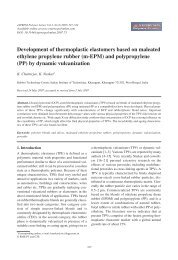
The die had a rectangular section (6 mm×60 mm)<br />
and a length equal to 200 mm, and contained a<br />
quartz transparent window (14 mm×80 mm) on<br />
two orthogonal faces (Figure 1) in order to meet the<br />
requirements <strong>of</strong> the PIV method. In a second step,<br />
the basic geometry was slightly modified by fixing<br />
a small obstacle (4 mm×8 mm×14 mm) on the bottom<br />
surface <strong>of</strong> the die. The maximum <strong>flow</strong> rate <strong>of</strong><br />
the extruder was 30 kg/h, which corresponds to a<br />
maximum average velocity <strong>of</strong> 20 mm/s and a maximum<br />
apparent shear rate <strong>of</strong> 20 s –1 . Melt and die<br />
temperatures were set at the same level (280 to<br />
320°C for polycarbonate and 220°C for polystyrene).<br />
The temperature control system <strong>of</strong> the die<br />
was that <strong>of</strong> the industrial <strong>extrusion</strong> machine. It is<br />
therefore necessarily less efficient than the temper-<br />
Figure 1. Extrusion die: a) overview, b) transverse section,<br />
c) adaptation device<br />
570
Fournier et al. – eXPRESS Polymer Letters Vol.3, No.9 (2009) 569–578<br />
ature control systems attached to laboratory devices<br />
such as capillary rheometers. That is why the<br />
experiments carried out on the industrial extruder<br />
have been always performed under the same conditions,<br />
after stabilization so as to reach a steady state<br />
and thus to limit this inconveniency.<br />
PIV equipment was supplied by Dantec Dynamics.<br />
The principles <strong>of</strong> this measurement technique can<br />
be found elsewhere [15]. The lighting was generated<br />
by a Nd:YAG laser emitting at 532 nm<br />
(green). Optical lenses are used to create a 1 mm<br />
thick laser sheet. A CCD camera recorded the pictures.<br />
Aluminum powder (average diameter:<br />
1.5 μm) was used as tracer at a weight concentration<br />
<strong>of</strong> 5 to 10·10 –4 %. This material was chosen due<br />
to its high light reflectivity that appeared adequate<br />
after comparison with others materials (talcum,<br />
glass spheres). The time between photographs was<br />
adapted to the <strong>extrusion</strong> <strong>flow</strong> rate and varied from<br />
5000 to 30000 μs. The size <strong>of</strong> the interrogation<br />
window (IW) was kept constant, equal to<br />
64×64 pixels (i.e. 558×558 μm). The observation<br />
zone covered 25 IW resp. 11 IW in the <strong>flow</strong> direction<br />
resp. in the transverse direction. The choice <strong>of</strong><br />
these parameters is the result <strong>of</strong> a compromise<br />
between the size <strong>of</strong> the gap to be observed, the<br />
<strong>image</strong> quality, the average displacement <strong>of</strong> the <strong>particle</strong>s<br />
between two successive <strong>image</strong>s and the mean<br />
<strong>flow</strong> rate.<br />
Rheological measurements were carried out on a<br />
rheograph (Göttfert) <strong>using</strong> 0.5 and 1 mm capillary<br />
dies with a L/D ratio <strong>of</strong> 20. Wall slip was determined<br />
<strong>using</strong> the classical Mooney’s method [17,<br />
18]. For a capillary <strong>flow</strong>, it is based on Equation<br />
(1):<br />
4V γ &<br />
s<br />
A = γ&<br />
A, S +<br />
(1)<br />
R<br />
where V s is the slip velocity, γ·A the apparent shear<br />
rate (calculated from <strong>flow</strong> rate Q and die radius R<br />
by Equation (2)) and γ·A,S the apparent shear rate<br />
corrected for slip, which is only a function <strong>of</strong> the<br />
wall shear stress (τ w ).<br />
4Q<br />
γ&<br />
A =<br />
3<br />
(2)<br />
πR<br />
At constant shear stress, the slip velocity can then<br />
be calculated from a plot <strong>of</strong> γ·A vs. 1/R, which is a<br />
straight line <strong>of</strong> 4V s slope. To apply this method, it is<br />
therefore necessary to measure the <strong>flow</strong> curves τ w<br />
vs. γ·A for capillaries <strong>of</strong> various diameters.<br />
Numerical simulations were performed <strong>using</strong> REM<br />
3D s<strong>of</strong>tware package supplied by Transvalor. This<br />
finite elements s<strong>of</strong>tware is dedicated to the three<br />
dimensional simulation <strong>of</strong> <strong>extrusion</strong> and injection<br />
molding processes and their variants (co-injection,<br />
co-<strong>extrusion</strong>, gas and water assisted injection molding).<br />
It contains a specific module based on a power<br />
law model (Equation (3)) to introduce wall slip in<br />
the computation.<br />
n<br />
τ = α·K·V s<br />
(3)<br />
with τ the shear stress, α the slip coefficient, K the<br />
consistency, V s the slip velocity and n the exponent<br />
<strong>of</strong> the power law.<br />
3. Results and discussion<br />
Two slightly different geometries were analyzed.<br />
The first corresponded to a basic <strong>flow</strong> in a rectangular<br />
die. It was used to implement and validate the<br />
method, and set the measurement parameters. It<br />
was also used to study the velocity pr<strong>of</strong>ile through<br />
the thickness <strong>of</strong> the die. In the second case, the <strong>flow</strong><br />
was disrupted by means <strong>of</strong> a geometrical discontinuity.<br />
This obstacle generated an abrupt step in the<br />
<strong>flow</strong> and a complex deviation <strong>of</strong> the latter. The<br />
resulting velocity pr<strong>of</strong>ile was then compared to<br />
numerical simulations introducing wall slip in the<br />
computation on the basis <strong>of</strong> rheological measurements.<br />
3.1. PIV measurements<br />
3.1.1. Simple <strong>flow</strong>s<br />
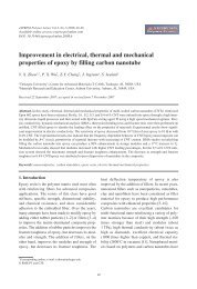
A typical example <strong>of</strong> a velocity field measured in<br />
the rectangular die for polycarbonate is presented<br />
in Figure 2. Figure 3 shows the pr<strong>of</strong>iles through the<br />
thickness <strong>of</strong> the die for the different <strong>flow</strong> rates that<br />
can be reached with the processing equipment.<br />
Though the velocity pr<strong>of</strong>iles appear globally as<br />
quadratic power laws as one could expect for Newtonian<br />
<strong>flow</strong>s (which is the case <strong>of</strong> polycarbonate in<br />
the range <strong>of</strong> temperature and <strong>flow</strong> rates covered by<br />
this study) between parallel plates, several peculiarities<br />
can be seen on these pr<strong>of</strong>iles. First, some<br />
velocity pr<strong>of</strong>iles are not symmetric with respect to<br />
the axis <strong>of</strong> the die. However it is worth reminding<br />
571
Fournier et al. – eXPRESS Polymer Letters Vol.3, No.9 (2009) 569–578<br />
Figure 2. Typical experimental velocity field through the<br />
die (temperature: 280°C, shear rate: 8.2 s –1 )<br />
that the experiments were carried out on an industrial<br />
machine, whose temperature regulation is not<br />
perfect and may be slightly non-symmetric. Secondly,<br />
the speed is non-zero at the wall and can represent<br />
a significant part <strong>of</strong> the maximum speed for<br />
the lowest <strong>flow</strong> rates (Figure 3b). Thirdly, the pr<strong>of</strong>iles<br />
measured at shear rates above 13 s –1 have a<br />
bell shape instead <strong>of</strong> a pure parabolic one as it<br />
appears at lower <strong>flow</strong> rates.<br />
The observations concerning wall slip are rather<br />
surprising if we consider the low shear rates<br />
(< 20 s –1 ) involved in these experiments. Nevertheless,<br />
the measurements are relevant since the <strong>flow</strong><br />
rate calculated from the velocity pr<strong>of</strong>ile and the one<br />
obtained from melt weight measurements at the<br />
exit <strong>of</strong> the die show a good match (Figure 4). Wall<br />
slip has to be there to get this match. Furthermore,<br />
the measurements close to the wall fit perfectly to<br />
Figure 3. Flow pr<strong>of</strong>iles for various shear rates (temperature:<br />
280°C): a) whole series <strong>of</strong> pr<strong>of</strong>iles,<br />
b) detail <strong>of</strong> the pr<strong>of</strong>iles at low shear rates<br />
Figure 4. Comparison <strong>of</strong> the <strong>flow</strong> rates calculated from<br />
the velocity pr<strong>of</strong>iles and measured by melt<br />
weighing at the die outlet<br />
the global velocity pr<strong>of</strong>ile, and the same result<br />
would have been obtained by extrapolating the wall<br />
velocity from the central part <strong>of</strong> the pr<strong>of</strong>ile. The<br />
measurements close to the wall are therefore reliable<br />
and we can fairly conclude that there is a significant<br />
slip at the wall within the spatial precision<br />
range <strong>of</strong> the measurement technique (0.2–0.3 mm).<br />
A non-slip layer thinner than the resolution <strong>of</strong> the<br />
system is obviously possible but such layer has not<br />
been reported in the literature even when 10 time<br />
more precise methods were used [9, 10].<br />
Furthermore, similar tests were punctually carried<br />
out with PS. The analysis <strong>of</strong> the measured velocity<br />
fields (in the same <strong>flow</strong> rate range) does not show<br />
wall-slip phenomena, the measured velocity at wall<br />
being not significant (
Fournier et al. – eXPRESS Polymer Letters Vol.3, No.9 (2009) 569–578<br />
Figure 5. Experimental (symbols and dashed lines) vs.<br />
theoretical (solid line) velocity pr<strong>of</strong>iles through<br />
the die (Newtonian isothermal model between<br />
infinite parallel plates)<br />
on an industrial extruder, the melt temperature is<br />
not fully controlled and depends on shear heating in<br />
the screw. Regarding the <strong>flow</strong>path length, the viscous<br />
shear heating may become significant, contrary<br />
to what is observed on laboratory devices<br />
such as rheometers. As a consequence, the melt<br />
temperature rises when the screw rotation speed<br />
and therefore the <strong>flow</strong> rate are increased. Temperature<br />
measurements at the die exit showed a discrepancy<br />
<strong>of</strong> about 20°C between shear rates <strong>of</strong> 3 and<br />
15 s –1 (Figure 6), whereas the shear heating<br />
induced temperature variations measured on the<br />
capillary rheometer remain lower than 2°C. This<br />
shear heating, which is important in industrial configurations,<br />
should generate more slip [16–18]. On<br />
the other hand, the results are presented vs. shear<br />
rate and not shear stress. The rise in temperature<br />
comes together with a decrease in viscosity and<br />
shear stress, and therefore a lower slip. In the particular<br />
case <strong>of</strong> polycarbonate considered in this<br />
study, the first phenomenon appears to be dominant,<br />
and, for a given apparent shear rate at the die<br />
wall, the reduction <strong>of</strong> the apparent shear stress (and<br />
thus the wall slip velocity) linked to the viscosity<br />
Figure 6. Wall slip velocity and melt temperature at the<br />
exit <strong>of</strong> the die vs. apparent shear rate (nominal<br />
temperature: 280°C)<br />
decrease is not enough to compensate the increase<br />
<strong>of</strong> the slip velocity induced by the temperature elevation.<br />
The distortion <strong>of</strong> the pr<strong>of</strong>iles at high <strong>flow</strong> rates<br />
(Figure 3a) can also be explained by thermal<br />
effects. Because <strong>of</strong> the shear heating <strong>of</strong> the melt<br />
(Figure 6), the temperature pr<strong>of</strong>ile through the die<br />
is no longer isothermal when the <strong>flow</strong> rate is<br />
increased. This temperature gradient comes<br />
together with other gradients <strong>of</strong> physical properties<br />
<strong>of</strong> the melt, especially its density and its refractive<br />
index. The melt acts therefore as a lens and deforms<br />
the <strong>image</strong>s that have to cross 30 mm <strong>of</strong> melt to exit<br />
the die and reach the recording camera. This was<br />
clearly visible at high <strong>flow</strong> rates because an apparent<br />
<strong>image</strong> <strong>of</strong> the die surfaces was visible away from<br />
the boundaries given by the steel surfaces. The<br />
higher the speed was, the narrower the apparent<br />
<strong>image</strong> was, which shows the temperature dependence<br />
<strong>of</strong> the phenomenon. This effect was partly<br />
corrected by resetting the walls position on the<br />
basis <strong>of</strong> their apparent <strong>image</strong> but it was impossible<br />
to have a perfect correction between these boundaries<br />
since the temperature gradient was unknown.<br />
This explains the peculiar shape <strong>of</strong> the velocity pr<strong>of</strong>iles.<br />
This is a physical phenomenon that cannot be<br />
avoided and that has to be taken into account when<br />
analyzing the results.<br />
3.1.2. Disrupted <strong>flow</strong>s<br />
In a second phase, the PC <strong>flow</strong> was disrupted by<br />
introducing a geometrical discontinuity. The results<br />
obtained with this configuration are presented in<br />
Figures 7 and 8. Figure 7 presents the observation<br />
from the side <strong>of</strong> the die, similar point <strong>of</strong> view to the<br />
one used in the previous section. In Figure 8, laser<br />
lighting and recording camera were swapped in<br />
order to study the <strong>flow</strong> from above at two different<br />
levels. Note that the observation window and the<br />
obstacle are much narrower than the total width <strong>of</strong><br />
the channel (14 mm vs. 60 mm) i.e. the polymer<br />
can <strong>flow</strong> beyond the observation window and the<br />
obstacle.<br />
These measurements give a good description <strong>of</strong> the<br />
deviation <strong>of</strong> the <strong>flow</strong> when passing the discontinuity.<br />
One can see the effect <strong>of</strong> a large step but also <strong>of</strong><br />
a small one. The lack <strong>of</strong> adjustment <strong>of</strong> the fixation<br />
screw generates a 0.5 mm-deep depression on the<br />
surface <strong>of</strong> the obstacle. This creates waves and<br />
573
Fournier et al. – eXPRESS Polymer Letters Vol.3, No.9 (2009) 569–578<br />
Figure 9. Combination <strong>of</strong> the different measurement and<br />
calculation results (for a given temperature)<br />
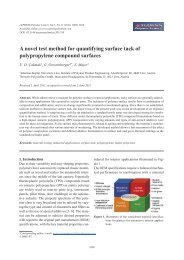
Figure 7. Velocity field in the vicinity <strong>of</strong> an obstacle (side<br />
view, <strong>flow</strong> from right to left): a) optical<br />
overview, b) velocity field<br />
speed changes in the <strong>flow</strong> above the obstacle,<br />
which are recorded on the side view (Figure 7). The<br />
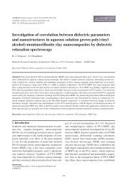
outline <strong>of</strong> this screw can also be distinguished on<br />
the top view (Figure 8c) through the distortion <strong>of</strong><br />
the velocity field. The observation from two<br />
orthogonal points gives quantitative information<br />
about the three-dimensional <strong>flow</strong>. In the next section,<br />
these results will be compared to numerical<br />
simulations.<br />
3.2. Rheological measurements and numerical<br />
simulations<br />
Since wall slip was pointed out in section 3.1.1. for<br />
polycarbonate, this phenomenon was taken into<br />
account in the numerical simulations. The numerical<br />
slip parameters were determined <strong>using</strong> rheometry.<br />
Figure 9 gives an overview <strong>of</strong> the way the<br />
experimental results and numerical simulations<br />
were combined. The parameters <strong>of</strong> the numerical<br />
slip law were first determined on the basis <strong>of</strong><br />
rheometry results, <strong>using</strong> the exponent m as it was<br />
measured and adjusting the slip coefficient α in<br />
order to get a good match between the numerical<br />
and the rheological slip velocity when simulating a<br />
capillary <strong>flow</strong>. Numerical simulations were then<br />
performed on geometries corresponding to the PIV<br />
die <strong>using</strong> the slip parameters determined at the previous<br />
step.<br />
Flow curves (Figure 10) were measured for different<br />
die diameters. Based on Mooney’s method, the<br />
discrepancy between these curves was used to calculate<br />
the slip velocity <strong>using</strong> the slope <strong>of</strong> the curve<br />
obtained when plotting the apparent shear rate vs.<br />
the reverse diameter at constant shear stress. Figure<br />
11 shows the evolution <strong>of</strong> the slip velocity with<br />
the apparent shear stress. One can see that slip is<br />
present and does not show any clear critical stress<br />
corresponding to the onset <strong>of</strong> slip down to<br />
0.04 MPa, the <strong>flow</strong> curves showing a progressive<br />
departure from each other (Figure 10). Wall slip is<br />
connected to shear stress through a power law<br />
(Equation (4)) within the range <strong>of</strong> shear stress covered<br />
by this study (0–0.18 MPa).<br />
Figure 8: Velocity field in the vicinity <strong>of</strong> an obstacle (top<br />
view, <strong>flow</strong> from right to left): a) optical<br />
overview, b) velocity field below the obstacle<br />
surface, c) velocity field above the obstacle<br />
Figure 10. Flow curves for two capillaries diameters at<br />
280°C<br />
574
Fournier et al. – eXPRESS Polymer Letters Vol.3, No.9 (2009) 569–578<br />
Figure 11. Slip velocity vs. apparent shear stress for different<br />
temperatures (capillary rheometry)<br />
Vs<br />
= α·<br />
τ<br />
m<br />
(4)<br />
Table 1 reports the parameters <strong>of</strong> the law for different<br />
temperatures. It appears that temperature has a<br />
limited influence on the exponent m whereas the<br />
coefficient α is strongly sensitive to it. For a given<br />
apparent shear stress, an increase in temperature<br />
induces a high increase in wall-slip velocity. For<br />
example, at an apparent shear stress <strong>of</strong> 0.1 MPa, the<br />
wall-slip velocity increases by 90% between 280<br />
and 300°C. The same trend was reported by<br />
Hatzikiriakos and Dealy [16, 17] in the case <strong>of</strong> high<br />
density polyethylene.<br />
The ranges <strong>of</strong> shear rates used for capillary measurements<br />
(25–300 s –1 ) and for PIV applied to <strong>extrusion</strong><br />
(
Fournier et al. – eXPRESS Polymer Letters Vol.3, No.9 (2009) 569–578<br />
Figure 14. Slip velocity vs. apparent shear rate: influence<br />
<strong>of</strong> the increase in melt temperature on the simulated<br />
wall slip<br />
adjusted accordingly by linear extrapolation<br />
between the rheological measurements at 280 and<br />
300°C. The simulated results obtained that way<br />
(Figure 14) are much closer to the experimental<br />
results, and also show the same wall-slip velocity<br />
stabilisation at higher shear rates as the one<br />
observed experimentally. Even if the difference<br />
between simulation and measurements still remains<br />
significant at higher shear rates, these results<br />
demonstrate that it is interesting and <strong>of</strong> prime<br />
importance to take the above-mentioned temperature-dependence<br />
in the slipping law.<br />
Figure 15 represents the numerical velocity pr<strong>of</strong>iles<br />
with and without slip. It definitely appears that the<br />
velocity pr<strong>of</strong>ile is significantly influenced by wall<br />
slip with reduction in the velocity range through the<br />
thickness and lower velocity gradients. Not taking<br />
slip into account can therefore lead to numerical<br />
simulations that are significantly different from the<br />
reality, not only in terms <strong>of</strong> velocity pr<strong>of</strong>iles but<br />
also concerning other important parameters <strong>of</strong> the<br />
process. For example, the inlet pressure is divided<br />
by two when wall slip is present (Figure 16).<br />
Figure 16. Simulated pressure at the entrance <strong>of</strong> the die<br />
vs. shear rate with and without wall slip<br />
In a second step, the <strong>extrusion</strong> through the die with<br />
the geometrical discontinuity was simulated. Wall<br />
slip was introduced into the calculation <strong>using</strong> the<br />
same parameter as the one determined in the simple<br />
<strong>flow</strong>. Figure 17a shows the field <strong>of</strong> the x-component<br />
(main <strong>flow</strong> direction) <strong>of</strong> the velocity. The evolution<br />
<strong>of</strong> the speed globally as well as near the wall<br />
shows a good agreement with what can be observed<br />
in Figure 8. Wall speed changes in accordance with<br />
the local fluctuation <strong>of</strong> the stress due to passing <strong>of</strong><br />
the complex obstacle.<br />
Comparison with the non-slip case (Figure 17b)<br />
emphasizes the regulating effect <strong>of</strong> stick. The<br />
velocity fluctuations are much less pronounced in<br />
the absence <strong>of</strong> slip since the speed at the wall is<br />
always zero and is not sensitive to shear stress<br />
changes generated by the geometrical discontinuity.<br />
For example, the velocity in the center <strong>of</strong> the<br />
gap above the obstacle does not show more than<br />
5% <strong>of</strong> variation along the obstacle in the stick condition<br />
whereas there is more than 30% decrease in<br />
velocity between the side and the center <strong>of</strong> the<br />
obstacle when wall slip is there. This shows that<br />
wall slip tends to destabilize the <strong>flow</strong> when passing<br />
geometrical singularities.<br />
Figure 18 shows the <strong>flow</strong> lines around the discontinuity<br />
seen from the side and from above at two different<br />
levels. The agreement with Figures 7 and 8 is<br />
good, which proves the relevance <strong>of</strong> both experi-<br />
Figure 15. Numerical velocity pr<strong>of</strong>iles through the thickness<br />
<strong>of</strong> the die without (solid lines) and with<br />
(dashed lines) wall slip<br />
Figure 17. Simulated x-velocity field around an obstacle<br />
with (a) and without (b) wall slip (center plane,<br />
shear rate: 3.3 s –1 )<br />
576
Fournier et al. – eXPRESS Polymer Letters Vol.3, No.9 (2009) 569–578<br />
measurements validated this approach, showing a<br />
quite good agreement <strong>of</strong> the wall velocity in industrial<br />
equipment with numerical simulations.<br />
Figure 18. Simulated <strong>flow</strong> lines around an obstacle a) 3D<br />
overview (background: x-velocity map),<br />
b) side view, c) top view above the obstacle,<br />
d) top view below the obstacle surface<br />
mental PIV measurements and numerical simulations.<br />
It is important to remember that the <strong>flow</strong> is<br />
complex with a real three dimensional behavior as<br />
shown in Figure 18a.<br />
4. Conclusions and outlook<br />
This study has shown the applicability <strong>of</strong> the PIV<br />
technique to characterize polymer <strong>flow</strong>s in an<br />
<strong>extrusion</strong> die in very constraining conditions: real<br />
polymer (and not model fluid), industrial equipment<br />
(machine, tooling), high temperature, pressure<br />
and velocity conditions. PIV was successfully<br />
used to analyze the <strong>flow</strong> pr<strong>of</strong>iles globally as well as<br />
for a detailed analysis <strong>of</strong> the surface phenomena in<br />
the case <strong>of</strong> a particular reference <strong>of</strong> polycarbonate.<br />
Furthermore, it was possible to highlight an<br />
unusual behavior <strong>of</strong> the polycarbonate investigated,<br />
characterized by a significant wall-slipping even at<br />
very low shear rate, confirmed by rheometry measurements.<br />
Numerical simulations <strong>using</strong> slip parameters<br />
determined on the basis <strong>of</strong> simple rheometrical<br />
measurements showed a good agreement with<br />
experimental direct observation at low shear rate.<br />
At higher shear rate, the necessity to introduce a<br />
temperature-dependence <strong>of</strong> the slip parameters has<br />
been shown. This requires a more extensive characterization<br />
<strong>of</strong> the temperature influence and the<br />
development <strong>of</strong> the adequate models to account for<br />
its effect more accurately in the simulation.<br />
Nonetheless, determining the numerical slip parameters<br />
on the basis <strong>of</strong> simple rheometrical measurements<br />
appeared, at least qualitatively, to be an<br />
interesting way to introduce wall slip in the simulation<br />
<strong>of</strong> <strong>flow</strong>s in more complex geometries. PIV<br />
Acknowledgements<br />
This work has been partly funded by the French Ministère<br />
de l’Économie des Finances et de l’Industrie, as part <strong>of</strong><br />
‘Réseau National Matériaux et Procédés’, project ‘Masther’.<br />
The authors also wish to thank Transvalor for supplying<br />
the simulation s<strong>of</strong>tware.<br />
References<br />
[1] Yokoi H., Hayashi T., Morikita N., Todd K.: Direct<br />
observation <strong>of</strong> jetting phenomena under a high injection<br />
pressure by <strong>using</strong> a prismatic-glass inserted<br />
mould. in ‘Proceedings <strong>of</strong> the SPE Annual Technical<br />
Conference ANTEC’88, Atlanta, USA’ 329–333<br />
(1988).<br />
[2] Yokoi H., Murata Y., Oka K., Watanabe H.: Visual<br />
analysis <strong>of</strong> weld line vanishing process by glassinserted<br />
mould. in ‘Proceedings <strong>of</strong> the SPE Annual<br />
Technical Conference ANTEC’91, Montreal, Canada’<br />
367–371 (1991).<br />
[3] Yokoi H., Nagami S., Kawasaki A., Murata Y.: Visual<br />
analysis <strong>of</strong> <strong>flow</strong> mark generation process <strong>using</strong> glassinserted<br />
mould. I. Micro-grooved <strong>flow</strong> marks. in ‘Proceedings<br />
<strong>of</strong> the SPE Annual Technical Conference<br />
ANTEC’94, San Francisco, USA’ 368–372 (1994).<br />
[4] Yokoi H., Deguchi Y., Sakamoto I., Murata Y.: Visual<br />
analyses <strong>of</strong> <strong>flow</strong> mark generation process <strong>using</strong> glassinserted<br />
mould. II. Synchronous <strong>flow</strong> marks with<br />
same phases on both top and bottom surfaces <strong>of</strong><br />
moulded samples. in ‘Proceedings <strong>of</strong> the SPE Annual<br />
Technical Conference ANTEC’94, San Francisco,<br />
USA’ 829–832 (1994).<br />
[5] Yokoi H., Han X.: Visualization analysis <strong>of</strong> melt <strong>flow</strong>ing<br />
behavior into micro-scale grooves during cavity<br />
filling process in injection molding. in ‘Proceedings <strong>of</strong><br />
the 21 st Annual Meeting <strong>of</strong> the Polymer Processing<br />
Society, Leipzig, Germany’ CD-ROM, SL 2.6, p8<br />
(2005).<br />
[6] Dowling D. R., Bress T. J.: Visualisation <strong>of</strong> injection<br />
moulding. in ‘Proceedings <strong>of</strong> the SPE Annual Technical<br />
Conference ANTEC’97, Toronto, Canada’ Vol III,<br />
3692–3696 (1997).<br />
[7] Nabialek J.: Monitoring and recording <strong>of</strong> the polymer<br />
<strong>flow</strong> in a mold cavity during the injection molding<br />
process. in ‘Proceedings <strong>of</strong> the 21 st Annual Meeting <strong>of</strong><br />
the Polymer Processing Society (PPS-21), Leipzig,<br />
Germany’ Paper P 13.7 (2005).<br />
577
Fournier et al. – eXPRESS Polymer Letters Vol.3, No.9 (2009) 569–578<br />
[8] Agassant J-F., Arda D., Combeaud C., Merten A.,<br />
Münstedt H., Mackley M. R., Robert L., Vergne B.:<br />
Polymer processing <strong>extrusion</strong> instabilities and methods<br />
for their elimination or minimization. in ‘Proceedings<br />
<strong>of</strong> the 21 st Annual Meeting <strong>of</strong> the Polymer Processing<br />
Society (PPS-21), Leipzig, Germany’ Paper<br />
KL 1.3 (2005).<br />
[9] Münstedt H., Schmidt M., Wassner E.: Stick and slip<br />
phenomena during <strong>extrusion</strong> <strong>of</strong> polyethylene melts as<br />
investigated by laser-Doppler <strong>velocimetry</strong>. Journal <strong>of</strong><br />
Rheology, 44, 413–427 (2000).<br />
DOI: 10.1122/1.551092<br />
[10] Robert L., Demay Y., Vergnes B.: Stick-slip <strong>flow</strong> <strong>of</strong><br />
high density polyethylene in a transparent slit die by<br />
laser Doppler <strong>velocimetry</strong>. Rheologica Acta, 43,<br />
89–98 (2004).<br />
DOI: 10.1007/s00397-003-0323-x<br />
[11] Mitsoulis E., Schwetz M., Münstedt H.: Entry <strong>flow</strong> <strong>of</strong><br />
LDPE melts in a planar contraction. Journal <strong>of</strong> Non-<br />
Newtonian Fluid Mechanics, 111, 41–61 (2003).<br />
DOI: 10.1016/S0377-0257(03)00012-0<br />
[12] Martyn M. T., Gough T., Spares S., Coates P. D., Zarloukal<br />
M.: Visualisation and analysis <strong>of</strong> LDPE melt<br />
<strong>flow</strong>s in a co<strong>extrusion</strong> geometry. in ‘Proceedings <strong>of</strong><br />
the SPE Annual Technical Conference ANTEC 2002,<br />
San Francisco, USA’ 937–941 (2002).<br />
[13] Yokoi H., Inagaki Y.: Dynamic visualisation <strong>of</strong> cavity<br />
filling process along the thickness direction <strong>using</strong> a<br />
laser light sheet technique. in ‘Proceedings <strong>of</strong> the SPE<br />
Annual technical Conference ANTEC’92, Detroit,<br />
USA’ 457–460 (1992).<br />
[14] Nigen S., El Kissi N., Piau J. M., Sadun S.: Velocity<br />
field for polymer melts <strong>extrusion</strong> <strong>using</strong> <strong>particle</strong> <strong>image</strong><br />
<strong>velocimetry</strong>: Stable and unstable <strong>flow</strong> regimes. Journal<br />
<strong>of</strong> Non-Newtonian Fluid Mechanics, 112, 177–<br />
202 (2003).<br />
DOI: 10.1016/S0377-0257(03)00097-1<br />
[15] Buchhave P.: Particle <strong>image</strong> <strong>velocimetry</strong> – status and<br />
trends. Experimentals Thermal and Fluid Science, 5,<br />
586–604 (1992).<br />
DOI: 10.1016/0894-1777(92)90016-X<br />
[16] Hatzikiriakos S. G., Dealy J. M.: Wall slip <strong>of</strong> molten<br />
high density polyethylene I. Sliding plate rheometer<br />
studies. Journal <strong>of</strong> Rheology, 35, 497–523 (1991).<br />
DOI: 10.1122/1.550178<br />
[17] Hatzikiriakos S. G., Dealy J. M.: Wall slip <strong>of</strong> molten<br />
HDPE. II. Capillary rheometer studies. Journal <strong>of</strong> Rheology,<br />
36, 703–741 (1992).<br />
DOI: 10.1122/1.550313<br />
[18] Maciel A., Salas V., Soltero J. F. A., Guzman J.,<br />
Manero O.: On the wall slip <strong>of</strong> polymer blends. Journal<br />
<strong>of</strong> Polymer Science Part B: Polymer Physics, 40,<br />
303–316 (2002).<br />
DOI: 10.1002/polb.10093<br />
578