Bivariate Frequency Analysis of Extreme Rainfall Events via Copulas
Bivariate Frequency Analysis of Extreme Rainfall Events via Copulas
Bivariate Frequency Analysis of Extreme Rainfall Events via Copulas

Create successful ePaper yourself
Turn your PDF publications into a flip-book with our unique Google optimized e-Paper software.
Seminar Presentation<br />
<strong>Bivariate</strong> <strong>Frequency</strong> <strong>Analysis</strong> <strong>of</strong><br />
<strong>Extreme</strong> <strong>Rainfall</strong> <strong>Events</strong> <strong>via</strong> <strong>Copulas</strong><br />
Shih-Chieh Kao<br />
Purdue University<br />
February 2007
Outline<br />
• Background and motivation<br />
• Brief introduction to copulas<br />
• Previous work<br />
• Selection <strong>of</strong> extreme events<br />
• <strong>Analysis</strong> <strong>of</strong> marginal distributions<br />
• <strong>Analysis</strong> <strong>of</strong> dependence structure<br />
• Model applications<br />
• Conclusions
Background and Motivation<br />
• <strong>Extreme</strong> rainfall behavior<br />
– Basis for hydrologic design<br />
– Conventionally analyzed only by “depth”<br />
– Pre-specified artificial duration (filter), not the real<br />
duration <strong>of</strong> extreme rainfall event<br />
– Hard to represent other rainfall characteristics, e.g.<br />
peak intensity<br />
• Definition <strong>of</strong> extreme event in multi-variate sense<br />
is not clear<br />
• Dependence exists between rainfall<br />
characteristics (e.g. volume(depth), duration,<br />
peak intensity)<br />
• Explore the use <strong>of</strong> copulas
Basic Probability Definitions<br />
• Univariate (for variable X)<br />
– Cumulative density function (CDF) and probability<br />
density function (PDF)<br />
F X<br />
• <strong>Bivariate</strong> (for variables X and Y)<br />
– joint-CDF and joint-PDF<br />
H XY<br />
( x, y)<br />
= P[ X ≤ x,<br />
Y ≤ y]<br />
hXY<br />
( x,<br />
y)<br />
– Marginal distirbutions<br />
f<br />
( x) = P[ X ≤ x]<br />
f<br />
X<br />
( x) = FX<br />
( x)<br />
( x) h ( x y)<br />
= ∫<br />
∞ −∞<br />
X XY<br />
,<br />
dy<br />
∂x∂y<br />
– Marginals (univariate CDF)<br />
x<br />
y<br />
u F ( x) f ( x)<br />
dx F ( y) f ( y)<br />
=<br />
X<br />
= ∫−<br />
∞<br />
X<br />
∂<br />
∂x<br />
=<br />
∂<br />
2<br />
H<br />
XY<br />
( y) h ( x y)<br />
∫ ∞ Y XY<br />
,<br />
−∞<br />
f<br />
( x,<br />
y)<br />
= dx<br />
v =<br />
Y<br />
= ∫−∞<br />
Y<br />
dy 0 ≤ u,<br />
v ≤ 1
f<br />
( ) ∫ ∞ X<br />
x = hXY<br />
( x, y)<br />
dy<br />
−∞<br />
f ( y) h ( x y)<br />
∫ ∞ Y XY<br />
,<br />
−∞<br />
= dx<br />
( x y)<br />
h XY<br />
,
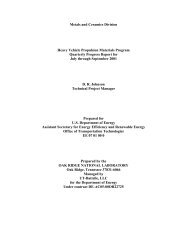
Concept <strong>of</strong> Dependence Structure<br />
• Conventionally quantified by the linear<br />
correlation coefficient ρ<br />
ρ<br />
XY<br />
=<br />
E<br />
[( X − x)( Y − y)<br />
]<br />
Std[ X ] Std[ Y ]<br />
– Can not correctly describe association between<br />
variables<br />
ρ=0.85 ρ=0.85 ρ=0.85<br />
– Only valid for Gaussian (or some elliptic) distributions<br />
– A better tool is required
Introduction to <strong>Copulas</strong><br />
• A copula C(u,v) is a function comprised <strong>of</strong> margins<br />
u & v from [0,1]×[0,1] to [0,1].<br />
– Sklar (1959) showed that for continuous marginals u and<br />
v, there exists a unique copula C such that<br />
H<br />
XY<br />
( x, y) = CUV<br />
( FX<br />
( x) , FY<br />
( y)<br />
) = CUV<br />
( u,<br />
v)<br />
– Transformation from [-∞,∞] 2 to [0,1] 2<br />
– Provides a complete description <strong>of</strong> dependence structure
Archimedean <strong>Copulas</strong> (I)<br />
• Archimedean <strong>Copulas</strong><br />
– There exists a generator φ(t), such that<br />
( C( u,<br />
v)<br />
)<br />
– When φ(t) = -ln(t), C(u,v) = uv. (Independent case)<br />
– Commonly used 1-parameter Archimedean <strong>Copulas</strong>:<br />
• Frank family<br />
• Clayton family<br />
( u) ϕ( v)<br />
ϕ = ϕ +<br />
ϕ<br />
• Genest-Ghoudi family<br />
ϕ<br />
−θt<br />
−θ<br />
() t = − ln[ ( e −1) ( e −1)<br />
]<br />
ϕ( t) = ( t<br />
−θ<br />
−1) θ<br />
1 θ<br />
() t = ( 1−<br />
t ) θ<br />
• Ali-Mikhail-Haq family<br />
ϕ() t = ln{ 1−θ<br />
( 1− t)<br />
t}<br />
[ ]<br />
C<br />
C<br />
C<br />
C<br />
( )<br />
( )(<br />
u, v = − ln<br />
⎜1+<br />
)⎟<br />
⎟<br />
−θ<br />
1<br />
⎛ −θ<br />
−θ<br />
− ⎞<br />
( u,<br />
v) = max⎜[ u + v −1] θ ,0⎟ ⎠<br />
{ ( [ θ<br />
] )} ,0<br />
θ<br />
1 θ θ 1 θ<br />
( u,<br />
v) = max1−<br />
( 1−<br />
u ) + ( 1−<br />
v )<br />
( u,<br />
v)<br />
1<br />
θ<br />
⎝<br />
=<br />
1−θ<br />
⎛<br />
⎝<br />
uv<br />
u<br />
e<br />
−θu<br />
−1<br />
e<br />
( 1−<br />
)( 1−<br />
v)<br />
e<br />
−θv<br />
−1<br />
−1<br />
⎞<br />
⎠
Archimedean <strong>Copulas</strong> (II)<br />
• Distribution function <strong>of</strong> copulas K C<br />
(t)=P[C UV<br />
(u,v)≤t]<br />
2<br />
( u,<br />
v) ∈ [ 0,1] | C( u,<br />
v)<br />
– Offers cumulative probability measure for<br />
ϕθ<br />
()<br />
( t)<br />
K C<br />
t = t −<br />
ϕ '()<br />
t<br />
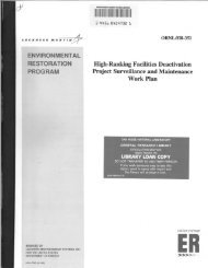
• Concordance measure - Kendall’s tau τ<br />
– 1: total concordance, -1: total discordance, 0: zero<br />
concordance<br />
– Sample estimator (c: concordant pairs, d: discordant<br />
pairs, n: number <strong>of</strong> samples)<br />
ˆ τ =<br />
θ<br />
[( X − X )( Y −Y<br />
) > ] − P[ ( X − X )( Y − ) 0]<br />
τ X , Y<br />
= P<br />
1 2 1 2<br />
0<br />
1 2 1<br />
Y2<br />
<<br />
⎛n⎞<br />
⎝ 2⎠<br />
( c − d ) ⎜ ⎟<br />
{ ≤ t}<br />
– For Archimedean copulas<br />
1 ϕθ<br />
( t)<br />
τ = 1+<br />
4∫<br />
dt<br />
0 ϕθ<br />
'()<br />
t<br />
– Non-parametric estimation <strong>of</strong> dependence parameter θ
τ= 0.66<br />
ρ= 0.85<br />
τ= 0.02<br />
ρ= 0.03<br />
τ= -0.65<br />
ρ= -0.84
Empirical <strong>Copulas</strong><br />
• Empirical copulas C n<br />
⎛ i j ⎞<br />
C n ⎜ , ⎟ =<br />
n<br />
a<br />
n<br />
⎝ n ⎠<br />
– a: number <strong>of</strong> pairs<br />
(x,y) in the smaple<br />
with x≤x (i) , y≤y (i)<br />
• Empirical distribution<br />
function K Cn<br />
⎛ k ⎞ b<br />
KC n<br />
⎜ ⎟ =<br />
⎝ n ⎠ n<br />
– b: number <strong>of</strong> pairs<br />
(x,y) in the sample<br />
with C n (i/n,j/n)≤k/n
Applications <strong>of</strong> <strong>Copulas</strong> in Hydrology<br />
• Flood <strong>Frequency</strong> <strong>Analysis</strong><br />
–Favreet al. (2004): Assessment <strong>of</strong> combined risk<br />
– De Michele et al. (2005): Dam spillway adequacy<br />
assessment<br />
– Grimaldi and Serinaldi (2006): The use <strong>of</strong> asymmetric<br />
copula in multi-variate flood frequency analysis<br />
– Zhang and Singh (2006): Conditional return period<br />
• Return period assessment using bivariate model<br />
– Salvadori and De Michele (2004): Concept <strong>of</strong><br />
secondary return period using distribution function K C<br />
• Probablistic structure <strong>of</strong> storm surface run<strong>of</strong>f<br />
– Kao and Govindaraju (2007): Quantifying the effect <strong>of</strong><br />
dependence between rainfall duration and average<br />
intensity on surface run<strong>of</strong>f
<strong>Copulas</strong> in <strong>Rainfall</strong> <strong>Frequency</strong> <strong>Analysis</strong><br />
• <strong>Rainfall</strong> frequency analysis<br />
– De Michele and Salvadori (2003, 2006)<br />
• Stochastic models for regular rainfall events<br />
• 2 rainfall stations in Italy with 7 years data<br />
– Grimaldi and Serinaldi (2006)<br />
• <strong>Extreme</strong> rainfall analysis<br />
• Relationship between design rainfall depth and the actual features<br />
<strong>of</strong> rainfall events<br />
• 10 rainfall stations in Italy with 7 years data<br />
– Zhang and Singh (2006)<br />
• <strong>Bivariate</strong> extreme rainfall frequency analysis using depth, duration<br />
and average intensity<br />
• 3 rainfall stations in Louisiana with 42 years data<br />
• Unanswered questions<br />
– Data used for analysis may not be sufficient<br />
– Definition <strong>of</strong> “extreme events” in multi-variate sense?<br />
– Can results be applied for a large region?
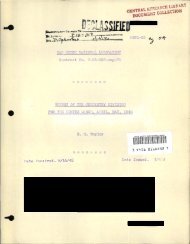
Data Source & Study Area<br />
• Nation Climate Data Center,<br />
Hourly Precipitation Dataset<br />
(NCDC, TD 3240 dataset)<br />
• 53 Co-operative <strong>Rainfall</strong> Stations<br />
in Indiana with record length<br />
greater than 50 years<br />
• Minimum rainfall hiatus: 6 hours<br />
• About 4800 events per station<br />
• Selected variables for analysis:<br />
– Depth (volume), P (mm)<br />
– Duration, D (hour)<br />
#<br />
# #<br />
#<br />
#<br />
#<br />
#<br />
#<br />
#<br />
#<br />
#<br />
#<br />
#<br />
#<br />
#<br />
#<br />
#<br />
#<br />
#<br />
#<br />
#<br />
#<br />
#<br />
# #<br />
#<br />
#<br />
#<br />
#<br />
#<br />
#<br />
#<br />
#<br />
# #<br />
#<br />
#<br />
#<br />
#<br />
#<br />
# #<br />
#<br />
#<br />
#<br />
#<br />
#<br />
#<br />
– Peak Intensity, I (mm/hour)<br />
#<br />
#<br />
• Marginals:<br />
– u=F P (p), v=F D (d), w=F I (i)<br />
#<br />
#<br />
#
Definitions <strong>of</strong> <strong>Extreme</strong> <strong>Events</strong><br />
• Hydrologic designs are usually governed by depth (volume)<br />
or peak intensity<br />
• Annual maximum volume (AMV) events<br />
– Longer duration<br />
• Annual maximum peak intensity (AMI) events<br />
– Shorter duration<br />
• Annual maximum cumulative probability (AMP) events<br />
– The use <strong>of</strong> empirical copulas C n between volume and peak intensity<br />
– Wide range <strong>of</strong> durations
<strong>Analysis</strong> <strong>of</strong> Marginal Distributions (I)<br />
• Candidate distributions<br />
– <strong>Extreme</strong> value type I (EV1)<br />
– Generalized extreme value (GEV)<br />
– Pearson type III (P3)<br />
– Log-Pearson type III (LP3)<br />
– Generalized Pareto (GP)<br />
– Log-normal (LN)<br />
• Parameters estimated primarily by maximum<br />
likelihood (ML) or method <strong>of</strong> moments (MOM)<br />
• Gringorton formula for empirical probabilities<br />
• Chi-square and Kolmogorov-Smirnov (KS) test<br />
with 10% significance level
<strong>Analysis</strong> <strong>of</strong> Marginal Distributions (II)<br />
AMV Rejection rate (%) <strong>of</strong> Chi-square test<br />
Rejection rate (%) <strong>of</strong> KS test<br />
events EV1 GEV P3 LP3 GP LN EV1 GEV P3 LP3 GP LN<br />
Depth, P 13.2 17.0 41.5 17.0 100 13.2 0.0 0.0 7.5 0.0 52.8 0.0<br />
Duration, D 13.2 15.1 24.5 37.7 100 22.6 1.9 0.0 7.5 0.0 22.6 0.0<br />
Intensity, I 15.1 17.0 45.3 20.8 100 11.3 0.0 0.0 1.9 0.0 54.7 0.0<br />
AMI Rejection rate (%) <strong>of</strong> Chi-square test<br />
Rejection rate (%) <strong>of</strong> KS test<br />
events EV1 GEV P3 LP3 GP LN EV1 GEV P3 LP3 GP LN<br />
Depth, P 5.7 3.8 62.3 3.8 100 1.9 0.0 0.0 11.3 0.0 45.3 0.0<br />
Duration, D 60.4 39.6 88.7 37.7 100 28.3 15.1 0.0 45.3 0.0 45.3 0.0<br />
Intensity, I 15.1 15.1 34.0 18.9 100 15.1 0.0 0.0 5.7 0.0 71.7 0.0<br />
AMP Rejection rate (%) <strong>of</strong> Chi-square test<br />
Rejection rate (%) <strong>of</strong> KS test<br />
events EV1 GEV P3 LP3 GP LN EV1 GEV P3 LP3 GP LN<br />
Depth, P 17.0 9.4 60.4 18.9 100 15.1 0.0 0.0 9.4 0.0 34.0 0.0<br />
Duration, D 24.5 26.4 64.2 26.4 100 18.9 0.0 0.0 13.2 1.9 15.1 0.0<br />
Intensity, I 7.5 17.0 43.4 18.9 100 9.4 0.0 0.0 1.9 3.8 62.3 0.0<br />
• EV1, GEV, LP3, LN provided better fit. GP provided<br />
the worst.<br />
• Fitting for duration <strong>of</strong> AMI events did not yield very<br />
good result<br />
• EV1 and LN could be recommended for use
<strong>Analysis</strong> <strong>of</strong> Dependence Structure (I)<br />
• Candidate Archimedean copulas<br />
– Frank family<br />
– Clayton family<br />
– Genest-Ghoudi family<br />
– Ali-Mikhail-Haq family<br />
• Non-parametric procedure for estimating<br />
dependence parameter<br />
• Examination <strong>of</strong> Goodness-<strong>of</strong>-fit<br />
– Distribution function K C (t)=P[C(u,v)≤t]<br />
– Diagonal section <strong>of</strong> copulas δ(t)=C(t,t)<br />
– Section with one marginal as median (one marginal<br />
equals 0.5)<br />
– Multidimensional KS test (Saunders and Laud, 1980)
Variation <strong>of</strong> Kendall’s τ<br />
τ PD τ DI τ PI<br />
mean stdev mean stdev mean stdev<br />
AMV events 0.183 0.084 -0.370 0.068 0.260 0.097<br />
AMI events 0.407 0.070 -0.011 0.096 0.405 0.070<br />
AMP events 0.324 0.078 -0.185 0.093 0.265 0.094
Variation <strong>of</strong> θ (Frank family)<br />
Frank<br />
θ UV θ VW θ UW<br />
family mean stdev mean stdev mean stdev<br />
AMV events 1.726 0.825 -3.824 0.909 2.546 1.063<br />
AMI events 4.333 1.003 -0.111 0.883 4.314 0.986<br />
AMP events 3.410 0.975 -1.863 0.927 2.389 1.029
Assessment <strong>of</strong> Copula Performance (I)
Assessment <strong>of</strong> Copula Performance (I)
<strong>Analysis</strong> <strong>of</strong> Dependence Structure (II)<br />
• The distribution function K C (t) provides the<br />
strictest examination <strong>of</strong> copulas<br />
• Clayton and Ali-Mikhail-Haq families performed<br />
well for positive dependence cases (C UV and<br />
C UW )<br />
• Frank family <strong>of</strong> Archimedean copulas<br />
– performed well for both positive and negative<br />
dependence<br />
– passed the KS test for entire Indiana at the 10%<br />
significant level<br />
– recommended for use in practice
Construct Joint Distribution <strong>via</strong> <strong>Copulas</strong><br />
• <strong>Bivariate</strong> stochastic models<br />
H ( p, d ) = C ( F ( p) , F ( d )) = C ( u v)<br />
H<br />
H<br />
PD UV P D<br />
UV<br />
,<br />
( d, i) = CVW<br />
( FD<br />
( d ),<br />
FI<br />
( i)<br />
) = CVW<br />
( v w)<br />
( p, i) = C ( F ( p) , F ( i)<br />
) = C ( u w)<br />
DI<br />
,<br />
PI UW P I<br />
UW<br />
,<br />
• Examples using Frank family and EV1 marginals
Application 1<br />
Estimate <strong>of</strong> depth for known duration (I)<br />
• For a known (or measured) d-hour event<br />
F<br />
P<br />
( p d −1<br />
< D ≤ d )<br />
=<br />
=<br />
H<br />
C<br />
PD<br />
UV<br />
( p,<br />
d ) − H<br />
PD<br />
( p,<br />
d −1)<br />
FD<br />
( d ) − FD<br />
( d −1)<br />
( FP<br />
( p) , FD<br />
( d )) − CUV<br />
( FP<br />
( p) , FD<br />
( d −1)<br />
)<br />
F ( d ) − F ( d −1)<br />
• Given return period T, the T-year, d-hour rainfall<br />
estimate p T will satisfy<br />
F ( p d −1<br />
< D ≤ d ) = 1−<br />
T<br />
P T<br />
1<br />
• Comparison between bivariate and univariate<br />
depth estimates<br />
– <strong>Bivariate</strong> using EV1 marginals and Frank family<br />
– Univariate counterpart using GEV distribution (Rao<br />
and Kao, 2006)<br />
D<br />
D
Estimate <strong>of</strong> depth for known duration (II)<br />
• Similar trends were observed for durations greater than<br />
10-hour, close to the univariate counterpart<br />
• For durations less than 10-hour<br />
– Univariate approach underestimated the rainfall depth<br />
– AMV estimates gave the highest value<br />
– AMI estimates should be the best, but fitting problem existed<br />
– AMP estimates are recommended<br />
• Average ratios for entire Indiana<br />
duration AMV/GEV AMP/GEV AMI/GEV<br />
1 1.98 1.51 1.18<br />
2 1.50 1.16 0.93<br />
3 1.33 1.04 0.86<br />
4 1.24 0.99 0.85<br />
6 1.14 0.96 0.89<br />
9 1.07 0.99 0.98<br />
12 1.05 1.03 1.04<br />
18 1.03 1.07 1.05<br />
24 1.03 1.08 1.03
Application 2<br />
Estimate <strong>of</strong> peak intensity for known duration (I)<br />
• For a known (or measured) d-hour event<br />
F<br />
I<br />
( i d −1<br />
< D ≤ d )<br />
=<br />
=<br />
H<br />
C<br />
• Given return period T, the T-year, d-hour rainfall<br />
estimate p T will satisfy<br />
F ( i d −1<<br />
D ≤ d ) = 1−<br />
T<br />
I T<br />
1<br />
DI<br />
VW<br />
F<br />
( d,<br />
i) − H<br />
DI<br />
( d −1,<br />
i)<br />
D<br />
( d ) − FD<br />
( d −1)<br />
( FD<br />
( d ),<br />
FI<br />
( i)<br />
) − CVW<br />
( FD<br />
( d −1 ),<br />
FI<br />
( i)<br />
)<br />
F ( d ) − F ( d −1)<br />
• Comparison between bivariate and univariate<br />
depth estimates<br />
– <strong>Bivariate</strong> using EV1 marginals and Frank family<br />
– Univariate counterpart using GEV depth with Huff<br />
(1967) temporal distribution derived at each station<br />
D<br />
D
Estimate <strong>of</strong> peak intensity for known duration (II)<br />
• Similar trends were observed between AMV,<br />
AMI, and AMP estimates.<br />
• AMI generally provided the largest estimates,<br />
unless positive dependence existed between D<br />
and I<br />
• Univariate approach<br />
– Peak intensity generated by GEV depth with Huff<br />
distribution is around 4-5 times larger than the<br />
average intensity<br />
– Followed the IDF relationship<br />
– Failed to capture peak intensity<br />
• AMP estimates are recommended
Application 3<br />
Estimate <strong>of</strong> peak intensity for known depth (I)<br />
• For extreme events greater than a threshold p<br />
F<br />
I<br />
( i P > p)<br />
=<br />
F<br />
I<br />
( i) − H<br />
PI<br />
( p,<br />
i)<br />
1−<br />
F ( p)<br />
w − CUW<br />
1 − u<br />
( u,<br />
w)<br />
• Conditional expectation E[I | P>p]<br />
E<br />
P<br />
∞<br />
∞ ∂<br />
[ I P > p] = ∫ if<br />
I<br />
( i P > p) di = ∫ i FI<br />
( i P > p)<br />
0<br />
=<br />
0<br />
∂i<br />
di
Conclusions (I)<br />
• Definition <strong>of</strong> extreme events<br />
– AMV events are generally <strong>of</strong> longer duration than<br />
AMP, following by AMI events. AMV events may<br />
therefore be less reliable for short durations.<br />
– For AMI definition, the hourly recording precision<br />
used in this study was found to be limiting<br />
– AMP criterion seems to be an appropriate indicator<br />
for defining extreme events<br />
• Marginal distributions<br />
– EV1, GEV, LP3, LN were found to be appropriate<br />
marginal models for extreme rainfall<br />
– EV1 and LN are recommended
Conclusions (II)<br />
• Dependence structure<br />
– Between P and D, positive correlated<br />
– Between D and I, generally negatively correlated<br />
– Between P and I, positive correlated<br />
– Frank family is recommended<br />
– Indiana rainfall may not be homogeneous in the multivariate<br />
sense<br />
• Estimate <strong>of</strong> depth for known duration<br />
– Similar results for durations larger than 10 hours<br />
– AMP estimates are recommended to use for<br />
durations less than 10 hours<br />
• Estimate <strong>of</strong> peak intensity for known duration<br />
– Conventional approach fails to capture the peak<br />
intensity<br />
– AMP definition is recommended
Thank you for listening.<br />
Questions?