Introductory Econometrics â Formula Sheet for the Final Exam
Introductory Econometrics â Formula Sheet for the Final Exam
Introductory Econometrics â Formula Sheet for the Final Exam

You also want an ePaper? Increase the reach of your titles
YUMPU automatically turns print PDFs into web optimized ePapers that Google loves.
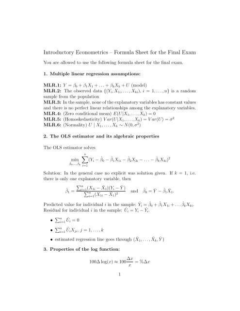
<strong>Introductory</strong> <strong>Econometrics</strong> – <strong>Formula</strong> <strong>Sheet</strong> <strong>for</strong> <strong>the</strong> <strong>Final</strong> <strong>Exam</strong><br />
You are allowed to use <strong>the</strong> following <strong>for</strong>mula sheet <strong>for</strong> <strong>the</strong> final exam.<br />
1. Multiple linear regression assumptions:<br />
MLR.1: Y = β 0 + β 1 X 1 + . . . + β k X k + U (model)<br />
MLR.2: The observed data {(Y i , X 1i , . . . , X ki ), i = 1, . . . , n} is a random<br />
sample from <strong>the</strong> population<br />
MLR.3: In <strong>the</strong> sample, none of <strong>the</strong> explanatory variables has constant values<br />
and <strong>the</strong>re is no perfect linear relationships among <strong>the</strong> explanatory variables.<br />
MLR.4: (Zero conditional mean) E(U|X 1 , . . . , X k ) = 0<br />
MLR.5: (Homoskedasticity) V ar(U|X 1 , . . . , X k ) = V ar(U) = σ 2<br />
MLR.6: (Normality) U | X 1 , . . . , X k ∼ N(0, σ 2 )<br />
2. The OLS estimator and its algebraic properties<br />
The OLS estimator solves<br />
n∑<br />
min (Y i − ˆβ 0 − ˆβ 1 X 1i − ˆβ 2 X 2i − . . . − ˆβ k X ki ) 2<br />
ˆβ 0 ,..., ˆβ k<br />
i=1<br />
Solution: In <strong>the</strong> general case no explicit was solution given. If k = 1, i.e.<br />
<strong>the</strong>re is only one explanatory variable, <strong>the</strong>n<br />
ˆβ 1 =<br />
∑ n<br />
i=1 (X 1i − ¯X 1 )(Y i − Ȳ )<br />
∑ n<br />
i=1 (X 1i − ¯X 1 ) 2 and ˆβ0 = Ȳ − ˆβ 1 ¯X1 .<br />
Predicted value <strong>for</strong> individual i in <strong>the</strong> sample: Ŷ i = ˆβ 0 + ˆβ 1 X 1i + . . . ˆβ k X ki .<br />
Residual <strong>for</strong> individual i in <strong>the</strong> sample: Û i = Y i − Ŷi.<br />
• ∑ n<br />
i=1 Ûi = 0<br />
• ∑ n<br />
i=1 ÛiX ji , j = 1, . . . , k<br />
• estimated regression line goes through ( ¯X 1 , . . . , ¯X k , Ȳ )<br />
3. Properties of <strong>the</strong> log function:<br />
100∆ log(x) ≈ 100 ∆x<br />
x<br />
= %∆x<br />
1
Predicting Y when <strong>the</strong> dependent variable is log(Y ):<br />
4. SST, SSE, SSR, R 2<br />
SST = ∑ n<br />
i=1 (Y i − Ȳ )2<br />
SSE = ∑ n<br />
i=1 (Ŷi − Ȳ )2<br />
SSR = ∑ n<br />
i=1 Û 2 i<br />
SST = SSE + SSR<br />
R 2 = SSE/SST = 1 − SSR/SST<br />
Ŷ adjusted = e σ2 /2 e ˆβ 0 + ˆβ 1 X 1 +... ˆβ k X k<br />
5. Variance of <strong>the</strong> OLS estimator, estimated standard error, etc.<br />
For j = 1, . . . , k:<br />
V ar( ˆβ j ) =<br />
σ 2<br />
SST Xj (1 − R 2 j ),<br />
where SST Xj = ∑ n<br />
i=1 (X ji− ¯X j ) 2 and Rj 2 is <strong>the</strong> R-squared from <strong>the</strong> regression<br />
of X j on all <strong>the</strong> o<strong>the</strong>r X variables. The estimated standard error of <strong>the</strong> ˆβ j ,<br />
j = 1, . . . , k, is given by<br />
√<br />
se(<br />
̂ ˆβ ˆσ<br />
j ) =<br />
2<br />
SST Xj (1 − Rj 2),<br />
where ˆσ 2 =<br />
SSR . n−k−1<br />
6. Simple omitted variables <strong>for</strong>mula:<br />
True model: Y = β 0 + β 1 X 1 + β 2 X 2 + U<br />
Estimated model: Y = β 0 + β 1 X 1 + V<br />
E( ˆβ 1 ) = β 1 + β 2<br />
cov(X 1 , X 2 )<br />
var(X 1 )<br />
2
7. Hypo<strong>the</strong>sis testing<br />
a. t-statistic <strong>for</strong> testing H 0 : β j = a<br />
ˆβ j − a<br />
ŝe( ˆβ j ) ∼ t(n − k − 1) if H 0 is true<br />
b. The F-statistic <strong>for</strong> testing hypo<strong>the</strong>ses involving more than one regression<br />
coefficient (“ur” = unrestricted, “r” = restricted, q = # of restrictions<br />
in H 0 , k = # of slope coefficients in <strong>the</strong> unrestricted regression)<br />
8. Heteroskedasticity<br />
(SSR r − SSR ur )/q<br />
SSR ur /(n − k − 1) ∼ F (q, n − k − 1) if H 0 is true<br />
Breusch-Pagan test <strong>for</strong> heteroskedasticity: Regress squared residuals on all<br />
explanatory variables and constant; test <strong>for</strong> joint significance of <strong>the</strong> explanatory<br />
variables.<br />
(F)GLS estimator: Let h(X 1 , . . . , X k ) = V ar(U|X 1 , . . . , X k ). Divide <strong>the</strong><br />
original model by <strong>the</strong> square root of h and do OLS. If h is unknown, one<br />
needs to model and estimate it as well.<br />
9. Linear probabiliy model<br />
V ar(U|X 1 , . . . , X k ) = (β 0 + β 1 X 1 + . . . β k X k )(1 − (β 0 + β 1 X 1 + . . . β k X k )).<br />
3