joint velocity inversion for pp and ps prestack depth imaging - PGS

More documents

Recommendations

Info

2 Theory and Methodology The proposed multi-component prestack depth migration flow is as following: (1) Build initial P-P and P-S velocity models and perform isotropic prestack depth migration for near offset P-P and P-S data. (2) Perform joint inversion on the migrated data to derive the vertical velocities that tie the depth of P-P and P-S images. The output from the inversion procedure will be the vertical depth, Z 0 , vertical P-wave velocity, Vp 0 , and vertical S-wave velocities, Vs 0 . (3) Update velocity model and re-run prestack depth migration for the same data. The resulting images between P-P and P-S should be depth consistent. (4) Use the velocity model obtained in step 3 to perform prestack depth migration for near to mid-offset data. If all depth image gathers are flat, then the data is isotropic and anisotropic processing is not required. If the image gathers are not flat, then anisotropy is implied. (5) Perform anisotropic parameter estimation. Vp 0 ,Vs 0 ,Z 0 Vp N,Z pp Vp N,Vs N,Z ps Vertical depth ∆Zpp ∆Zps Isotropic P-P image Figure 1. The mismatches between isotropic P-P and P-S images and vertical depth in the VTI medium. Our strategy for the anisotropic parameter estimation is depicted in Figure 1. We first perform P-P isotropic velocity focusing using the velocity model derived in step 3. Second, we stack the data and measure the depth, Z pp (see Figure 1). Third, we measure the depth difference between the vertical depth (Z 0 ) and isotropic P-P depth (Z pp ). Finally, we use this information to estimate the anisotropic parameter δ that can be expressed, to the first order approximation, as Z pp − Z 0 ∆Z pp δ ≈ = . Z 0 Z 0 where Z 0 is the vertical depth given by joint velocity inversion in step 2. Similarly, for the P-S anisotropic parameter, σ, we can approximate it by the following expression ∆Z 2 pp 2 γ ∆Z 0 pp σ ≈ γ 0 ( ) [ + 1] Z 2 Z 0 where γ 0 (=Vp 0 /Vs 0 ) is the ratio of the vertical P-wave velocity to the vertical S-wave velocity. Once these anisotropic parameters are determined, we can perform the final anisotropic prestack depth migration that requires Vp 0 , Vs 0 , δ, and σ. In summary, the depth consistent joint velocity inversion provides three critical parameters for the estimation of anisotropic parameters in presence of anisotropy: the vertical depth, Z 0 , vertical P-wave velocity, Vp 0 , and vertical S-wave velocities, Vs 0 . 0 Isotropic P-S image
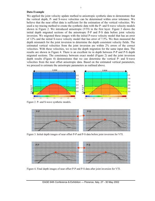
3 Data Example We applied the joint velocity update method to anisotropic synthetic data to demonstrate that the vertical depth, P- and S-wave velocities can be determined within error tolerance. We believe that the near offset data is sufficient for the estimation of the vertical velocities. We used a ray-tracing method to create the synthetic data with the P- and S-wave velocity models shown in Figure 2. We introduced anisotropic (VTI) in the first layer. Figure 3 shows the initial depth migrated sections of the anisotropic P-P and P-S data before joint velocity inversion. We migrated these images with the initial P-wave velocity model that has an error of 12% and the initial S-wave velocity model that has error of 7.5%. We then measured the depth mismatch for the joint inversion to determine the depth consistent velocity fields. The estimated vertical velocities from the joint inversion are within 2% errors of the correct velocities. With these velocities, we re-run the depth migration for the same input data. The results are shown in Figure 4. There is an excellent tie in depth between P-P and P-S depth migrated sections. The consistency between exact model (Figure 2) and the joint inversion depth results (Figure 4) demonstrates that we can determine the vertical P- and S-wave velocities from the near offset anisotropic data. Based on the estimated vertical parameters, we proceed to estimate the anisotropic parameters as outlined above. 5.0KM 5.0KM 0.5 0.5 1.0 1.0 1.5 1.5 D ep th (K M) 2.0 2.5 3.0 D ep th (K M) 2.0 2.5 3.0 Figure 2. P- and S-wave synthetic models. P-P P-S Figure 3. Initial depth images of near offset P-P and P-S data before joint inversion for VTI. P-P P-S Figure 4. Final depth images of near offset P-P and P-S data after joint inversion for VTI. EAGE 64th Conference & Exhibition — Florence, Italy, 27 - 30 May 2002
Page 1: 1 JOINT VELOCITY INVERSION FOR P-P

joint velocity inversion for pp and ps prestack depth imaging - PGS

You also want an ePaper? Increase the reach of your titles

Delete template?

Save as template?