OTC 16945 True 3D Data-driven Multiple Removal ... - PGS

OTC 16945 

True 3D Data-driven Multiple Removal: Acquisition & Processing Solutions 

Roald van Borselen, Rob Hegge and Michel Schonewille / PGS Geophysical 

Copyright 2004, Offshore Technology Conference 

This paper was prepared for presentation at the Offshore Technology Conference held in 

Houston, Texas, U.S.A., 3–6 May 2004. 

This paper was selected for presentation by an OTC Program Committee following review of 

information contained in an abstract submitted by the author(s). Contents of the paper, as 

presented, have not been reviewed by the Offshore Technology Conference and are subject to 

correction by the author(s). The material, as presented, does not necessarily reflect any 

position of the Offshore Technology Conference or officers. Electronic reproduction, 

distribution, or storage of any part of this paper for commercial purposes without the written 

consent of the Offshore Technology Conference is prohibited. Permission to reproduce in print 

is restricted to an abstract of not more than 300 words; illustrations may not be copied. The 

abstract must contain conspicuous acknowledgment of where and by whom the paper was 

presented. 

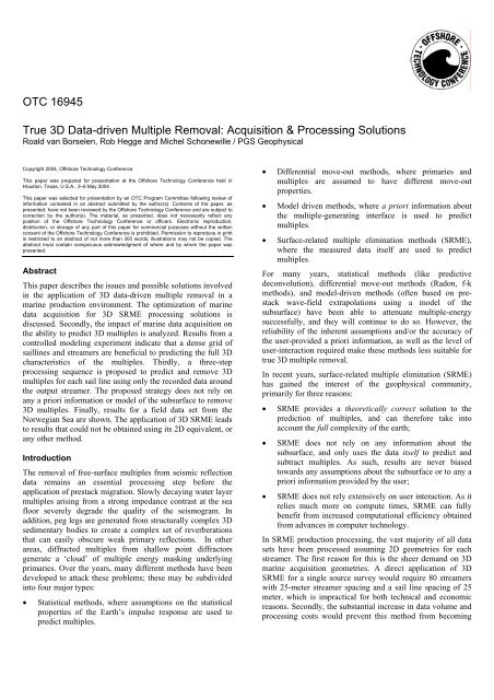
Abstract 

This paper describes the issues and possible solutions involved 

in the application of 3D data-driven multiple removal in a 

marine production environment. The optimization of marine 

data acquisition for 3D SRME processing solutions is 

discussed. Secondly, the impact of marine data acquisition on 

the ability to predict 3D multiples is analyzed. Results from a 

controlled modeling experiment indicate that a dense grid of 

saillines and streamers are beneficial to predicting the full 3D 

characteristics of the multiples. Thirdly, a three-step 

processing sequence is proposed to predict and remove 3D 

multiples for each sail line using only the recorded data around 

the output streamer. The proposed strategy does not rely on 

any a priori information or model of the subsurface to remove 

3D multiples. Finally, results for a field data set from the 

Norwegian Sea are shown. The application of 3D SRME leads 

to results that could not be obtained using its 2D equivalent, or 

any other method. 

Introduction 

The removal of free-surface multiples from seismic reflection 

data remains an essential processing step before the 

application of prestack migration. Slowly decaying water layer 

multiples arising from a strong impedance contrast at the sea 

floor severely degrade the quality of the seismogram. In 

addition, peg legs are generated from structurally complex 3D 

sedimentary bodies to create a complex set of reverberations 

that can easily obscure weak primary reflections. In other 

areas, diffracted multiples from shallow point diffractors 

generate a ‘cloud’ of multiple energy masking underlying 

primaries. Over the years, many different methods have been 

developed to attack these problems; these may be subdivided 

into four major types: 

• Statistical methods, where assumptions on the statistical 

properties of the Earth’s impulse response are used to 

predict multiples. 

• Differential move-out methods, where primaries and 

multiples are assumed to have different move-out 

properties. 

• Model driven methods, where a priori information about 

the multiple-generating interface is used to predict 

multiples. 

• Surface-related multiple elimination methods (SRME), 

where the measured data itself are used to predict 

multiples. 

For many years, statistical methods (like predictive 

deconvolution), differential move-out methods (Radon, f-k 

methods), and model-driven methods (often based on prestack 

wave-field extrapolations using a model of the 

subsurface) have been able to attenuate multiple-energy 

successfully, and they will continue to do so. However, the 

reliability of the inherent assumptions and/or the accuracy of 

the user-provided a priori information, as well as the level of 

user-interaction required make these methods less suitable for 

true 3D multiple removal. 

In recent years, surface-related multiple elimination (SRME) 

has gained the interest of the geophysical community, 

primarily for three reasons: 

• SRME provides a theoretically correct solution to the 

prediction of multiples, and can therefore take into 

account the full complexity of the earth; 

• SRME does not rely on any information about the 

subsurface, and only uses the data itself to predict and 

subtract multiples. As such, results are never biased 

towards any assumptions about the subsurface or to any a 

priori information provided by the user; 

• SRME does not rely extensively on user interaction. As it 

relies much more on compute times, SRME can fully 

benefit from increased computational efficiency obtained 

from advances in computer technology. 

In SRME production processing, the vast majority of all data 

sets have been processed assuming 2D geometries for each 

streamer. The first reason for this is the sheer demand on 3D 

marine acquisition geometries. A direct application of 3D 

SRME for a single source survey would require 80 streamers 

with 25-meter streamer spacing and a sail line spacing of 25 

meter, which is impractical for both technical and economic 

reasons. Secondly, the substantial increase in data volume and 

processing costs would prevent this method from becoming

2 OTC 

economically viable. However, due to new insights in the 

optimization of data acquisition, increased computer 

performance, and a better understanding of the fundamental 

steps in the reconstruction of missing data, the industry is now 

moving rapidly towards applying the full 3D implementation 

of SRME (see, for example, Hokstad and Sollie (2003), and 

Kleemeyer et al. (2003)). 

This paper presents an integrated strategy of the application of 

3D SRME in a production environment. In the first part, 

acquisition-related issues are discussed. It is shown how data 

can be acquired optimally for the prediction of 3D multiples. 

Also, the impact of data acquisition on the ability to predict 

3D multiples using SRME is investigated. In the second part, a 

processing strategy is presented that can be applied to most 3D 

data sets. Finally, the proposed processing strategy is applied 

to a field data set from the Norwegian Sea. 

Acquisition design criteria for 3D SRME 

To understand the impact of data acquisition on the ability to 

predict multiples, it is important to realize how multiples are 

predicted using SRME. Figure 1 shows how a typical freesurface 

multiple can be predicted by linking (adding) the 

raypaths of two events that are present in the measured data. 

This linkage is established through a convolution in time, and 

the actual position where the linkage takes place is called a 

‘multiple contribution’. Note that in order to establish the link, 

both source and receiver data must be available. To predict the 

multiple trace containing all free-surface multiples that belong 

to a source and receiver pair, all convolution results at all 

multiple-contribution locations have to be summed. In 

practice, after discretization of the wavefield, traces from a 3D 

common shot gather need to be convolved with all traces from 

a 3D common receiver gather, and summed. For the correct 

prediction of 3D multiples, the sampling of both the inline and 

crossline source and receiver locations needs to satisfy the 

Nyquist criteria. In addition, the aperture of the available data 

should be sufficient to include all relevant subsurface 

reflections, i.e. the Fresnel zone (Van Dedem et al, 2001). 

Figure 2 shows the ideal distribution of multiple contributions, 

where the aperture of the recorded data extends indefinitely. In 

practice, only a sparse distribution of multiple contributions in 

the crossline direction is obtained, as sources are only 

available on a sparse grid. In addition, only a limited crossline 

aperture is available due to the finite number of streamers 

used. It is remarked that the inline distribution of multiple 

contributions is, in general, sufficient. 

The key to the successful application of 3D SRME is to 

maximize the number of multiple contributions in the crossline 

direction, to obtain a regular distribution of the multiple 

contributions, and to maximize the crossline distance 

(aperture) between the two outer multiple contributions. 

In marine data acquisition, the main factors controlling the 

crossline spatial characteristics of the survey are the 

• Number of streamers, 

• Streamer separation, 

• Sail line spacing, 

• Source configuration (single or dual source, and the 

spacing between two sources when shooting in dual 

source mode). 

Figure 3a shows a conventional 8-streamer dual source 

configuration, where the sailline spacing is such that 

midpoints are not overlapping in the crossline direction. For 

the source and receiver combination depicted, the available 

three crossline multiple contribution positions are shown. Only 

at the positions highlighted can raypaths be connected to 

predict the 3D multiples. Note that changing the streamer 

spacing only affects the aperture between the two outer 

multiple contributions; it does not change the actual number of 

multiple contributions. In Figure 3b, it is shown how the 

number of multiple contributions increases when the number 

of streamers is increased while keeping the sailline spacing 

constant (streamer overlap). Note that, for this source and 

receiver combination, the additional two streamers on each 

side doubles the number of multiple contributions to six. Note 

also that the aperture between the multiple contributions has 

doubled as well. Figure 3c shows that by decreasing the sail 

line spacing by 50%, the number of multiple contributions can 

be increased further to eleven. Additionally, the aperture 

between the multiple contributions has increased slightly. As 

can be seen, the multiple contributions are now equally 

distributed over the aperure due to the additional intermediate 

saillines. Finally, in Figure 3d, it is shown how the number of 

multiple contributions changes when a single source 

configuration is used. Comparing this with Figure 3b (the 

same number of streamers and equal sailline spacing), a 

decrease in the number of multiple contributions is detected as 

the pairs of closely spaced contributions now have become 

single multiple contributions. However, it is noted that the 

distribution of the remaining contributions over the crossline 

aperture remains the same. 

Acquisition modeling 

To investigate the optimal acquisition geometry for the 

application of 3D SRME, an acquisition modeling tool was 

developed. 

Figure 4 shows the output of a simple modeling tool that was 

designed to compute the relevant diagnostics for the four 

acquisition geometries shown in Fig. 3. For each of the 

geometries, the first bar shows the number of contributions for 

the acquisition geometry under consideration. In this 

calculation, all sources within a midpoint spacing from the 

receiver line are taken into account. The other bars display the 

number of double contributions (i.e. number of secondary 

sources that are covered more than once), and the maximum 

crossline offsets to both sides that are involved in the multiple 

prediction, expressed in number of streamer intervals. From 

Fig. 4, it can be seen that by increasing the number of 

streamers and by reducing the sailline spacing, the number of 

multiple contributions increases for all streamers, where the 

highest number of multiple contributions occur at the inner 

streamers. Note from Fig. 4d that, even with some subsurface 

overlap, single source configurations leads to the situation

OTC 3 

where only two multiple contributions are available to predict 

3D multiples for the outer streamers. 

It should be noted that for a sailline spacing larger than twice 

the streamer separation, the amount of contributions can be 

increased artificially by applying some lateral shifts. In this 

way, one source of a neighboring streamer will act as 

secondary source for the two closest streamers. 

It is also remarked that the findings are independent of the 

actual streamer spacing as long as the sail line spacing is an 

integer multiple of the streamer spacing to obtain a repeatable 

pattern. The number of contributions will remain the same; 

only the crossline offsets and aperture will change 

accordingly. 

Finally, for dual source configurations, increasing the spacing 

between two sources may lead to a significant increase in both 

the aperture and the number of multiple contributions. 

However, this only applies to the hypothetical (and extremely 

uneconomical) case where the streamer spacing equals the sail 

line spacing. By putting both sources on one side of the 

streamers, the number of multiple contributions is reduced 

considerably. The contributions become very non-symmetric, 

which will be non-ideal for any 3D SRME implementation. 

The impact of acquisition on the prediction of 3D multiples 

In this subsection, the impact of the distribution of multiple 

contributions on the ability to predict 3D multiples is 

investigated. Because of the simplicity of the model used, 

insight is obtained in the general capabilities of interpolation 

and/or reconstruction methods to predict 3D multiples when 

only sparse data are available. 

In this example, the subsurface model consists of one plane 

layer dipping 4 degrees in the crossline direction only. Data 

were modeled for a dual source 16-streamer configuration 

with 50 meter streamer separation, with 200 meter and 400 

meter sailline separation respectively. Note that for this 

streamer configuration, 400 meter sail line spacing gives 

conventional sub-surface coverage with no duplication in the 

crossline direction. Figure 5a shows the ideal crossline 

multiple contribution gather for a source and receiver 

combination with 0 meter inline offset and 12.5 meter 

crossline offset. Figures 5b-c show, for the same source and 

receiver combination, the 7 and 3 crossline multiple 

contributions available for a 200 and 400 meter sailline 

separation respectively. Figure 6a shows a common shot 

gather for the inner streamer, and Fig. 6b shows the 

corresponding multiples, predicted using a 2D SRME 

approach. Figure 6c shows the ideal 3D multiples, and Figs. 

6d-e show the reconstructed multiples from the 200 and the 

400 meter sailline configuration respectively. Note that for 

both configurations, the 3D multiples were reconstructed 

satisfactory. Figures 7 and 8 shows the same results for the 

outer streamer. Note from Fig. 7b-c that the 5 contributions 

from the 200 meter sailline configuration (spaced at –362.5, – 

212.5, –162.5, –12.5 and 37.5 meters) are more equally 

distributed in the crossline direction than the 3 contributions 

from the 400 meter sailline configuation (spaced at –362.5, – 

12.5 and 37.5 meters). From Fig. 8b it can be seen that the 2D 

multiples are predicted too late in time. Also note that the 

results for the 200 meter sailline separation, shown in Figure 

8d, are significantly better then for the 400 meter separation 

shown in Figure 8e. This is due both to the increased number 

of contributions available (5 contributions for the 200 meter 

sailline separation versus 3 for the 400 meter separation), and 

the better distribution of the multiple contributions over the 

total aperture from the 200 meter configuration. However, for 

the data with 400 meter sailline separation, the second 

multiple is predicted much better than with 2D SRME, and 

although the wavelet of the first multiple is distorted, the 

timing is good. Therefore we would still expect 3D SRME to 

perform better than 2D SRME, even for the outer streamer. 

Recommendations for acquisition 

In 3D data-driven multiple removal, the multiple contributions 

(defined as locations where both receiver and source data are 

available) are the only data available to predict the 3D 

multiples. Hence, the distribution of multiple contributions 

will govern the quality of the final predicted 3D multiple trace. 

Results from synthetic modeling indicate that a denser grid of 

multiple contributions leads to a better prediction of the 3D 

multiples. 

During marine acquisition, the distribution of the crossline 

multiple contributions can be optimized for the application of 

3D SRME by 

• Shooting overlap (by increasing the number of streamers 

while keeping the sailline spacing constant); 

• Decreasing the sailline spacing; 

• Keeping the sailline spacing an integer multiplication of 

the streamer spacing; 

• Increasing the spread length 

For a more complex subsurface, it is therefore recommended 

to create a dense grid of multiple contributions with sufficient 

aperture to reconstruct the full complexity of the 3D multiples 

successfully. 

A processing strategy for 3D SRME 

This section describes an efficient processing sequence to 

apply 3D SRME in a production environment. A three-step 

sequence is proposed to predict and remove 3D multiples for 

each sail line using only the recorded data around the output 

streamer. Even though the proposed sequence will benefit 

from any form of acquisition optimization, the strategy is 

designed to handle 3D data sets that were acquired from 

conventional marine acquisition. The three steps involved are 

discussed in the following three subsections. 

Step 1: Pre-processing 

The pre-processing sequence starts with an analysis of the 

navigation data to investigate the positioning of the source and 

receivers. When irregularities (due to feathering and other 

positioning errors, such as drop-outs) are severe, wavefield 

regularization should be applied as part of the pre-processing 

sequence to position sources and receivers onto a regular pre-


defined grid. A data-driven regularization method, such as 

described in Schonewille et al. (2003) that uses the exact 

source- and receiver coordinates and allows for regularization 

to any user-defined grid is preferred. The proposed preprocessing 

sequence is very similar to the well-established 

pre-processing for the application of 2D SRME to marine data. 

The sequence includes: the removal of the direct wave and its 

surface reflection, the removal of non-physical noise and the 

directivity effects from source- and receiver arrays (optional), 

the recovery of missing shots and intermediate missing traces, 

shot interpolation (optional), and the extrapolation to zero 

offset of the inline component of the offsets. It is remarked 

that, after the optimal sequence and parameterizations have 

been found, all steps can be integrated into standardized flows 

to increase computational efficiency, and to minimize user 

interaction. 

Step 2: Multiple prediction through reconstruction in the 

crossline direction 

After pre-processing, the stacking of the multiple-contribution 

traces is carried out in two steps, first in the inline direction 

and secondly in the cross-line direction. Stacking of the 

multiple contribution traces in the inline direction is 

straightforward, as the sampling after pre-processing is 

sufficient. However, a direct Fresnel summation in the 

crossline direction leads to artifacts due to aliasing and 

insufficient aperture. Instead, the crossline summation is 

carried out implicitly through a reconstruction of the Fresnel 

zone, from a sparse-inversion based estimation of hyperbolic 

or parabolic events, with discrete curvatures and apex 

positions. 

In the literature, three methods for sparse-inversion based 

Fresnel zone reconstruction have been described: 1) using a 

time domain hyperbolic Radon transform (van Dedem and 

Verschuur, 2001); 2) using a frequency domain parabolic 

Radon transform (Hokstad and Sollie 2003); and 3) 

interpolation using Stolt migration operators (Trad, 2003). The 

time-domain approach has been shown to provide good results 

for 3D SRME, but is rather expensive. The frequency domain 

approach is computationally much more efficient, and has 

been shown to provide a good uplift compared with 2D SRME 

(Hokstad, 2003). However, using the frequency domain 

approach, only sparseness in the spatial direction can be 

enforced (Cary 1998, Trad 2003). As a result, for more 

complex data with events at many different apex positions, 

results may not be as good as with the time-domain approach. 

Interpolation with Stolt operators can provide sparseness in 

both time and space. The basic algorithm is computationally 

very efficient, but shows artifacts. These artifacts can be 

reduced, but this does increase the computational costs 

somewhat. This is a relatively new technique, and the 

suitability for 3D SRME is under further investigation. 

As the reconstruction has to be carried out for all source and 

receiver combinations, computational efficiency is vital for the 

economical viability of sparse-inversion based 3D SRME. In 

this paper, an approach is used that is based on the standard 

time domain approach described by van Dedem and Verschuur 

(2001) but which is much more computationally efficient. The 

computational speedup has been achieved through more 

efficient sparse matrix computations in a modified conjugate 

gradient scheme, and a data driven reduction of the model 

space. The results are comparable to those from using the 

standard time domain approach, and show significant 

improvements over any 2D implementation. 

After stacking the multiple-contribution traces in the Fresnel 

zone, a single trace with the corresponding predicted multiples 

is obtained, which can be used in the last step: the adaptive 

subtraction of the predicted multiples from the input data. 

Step 3: Adaptive subtraction of predicted multiples 

In the last step, the predicted free-surface multiples are 

subtracted from the input data using the minimum energy 

criterion, which states that the total energy after subtraction of 

the multiples should be minimized. In adaptive subtraction 

techniques, the predicted multiples are removed using Wiener 

filters designed in overlapping windows. In general, great care 

must be taken in choosing the filter length and the window 

size. If the filter length is too long, it is possible to remove 

primaries. Also, choosing too small a design window may lead 

to primary energy being affected when multiples and primaries 

are interfering. In 3D geometries, the application of 2D 

multiple prediction methods leads to multiples that are 

predicted too late in time. Using a 3D prediction scheme, the 

timing of the predicted multiples is better aligned with the 

multiples in the input data, leading to better removal of 

multiples. The more accurate timing of the predicted multiples 

allows the use of more conservative parameters in the adaptive 

subtraction, giving better preservation of primary energy. 

Field data example from the Norwegian Sea 

In this section, results from a 3D data set from the Norwegian 

Sea are shown. Data were shot in a dual-source 10-streamer 

configuration, with a 100 meter streamer separation and 500 

meter sailline separation. Results for a single offset line for 

one of the streamers have already been presented in Van 

Dedem and Verschuur (2001). Here, a total of 159 offset 

planes with a spacing of 12.5 meters were processed to allow 

further prestack processing after the application of 3D SRME. 

Figure 9 shows the results for a typical shot gather. Figure 9a 

shows the input gather after pre-processing. Figure 9b-c show 

the predicted multiples after 2D and 3D SRME respectively. A 

comparison indicates that, where the 2D multiples have all 

been predicted too late in time, the timing of the 3D predicted 

multiples is almost perfect. Figures 9d-e show the results after 

adaptive subtraction using the 2D and 3D predicted multiples 

respectively. It is remarked that a very mild adaptive 

subtraction approach was used in order to preserve the primary 

energy as much as possible. Note the much-improved removal 

of multiple-energy using the 3D predicted multiples. As a 

result, the remaining primaries have become much more 

visible. Figure 10 shows the same comparison for an inline at 

stack level. Note again the difference in timing between the 

2D and 3D predicted multiples, shown in Figs. 10b and c. As a 

result, after adaptive subtraction, the 3D result compares 

favorably to the 2D results. Both the first-order water bottom 

multiple (between 1.0 and 1.2 second), and the reverberations


off the elevated structure between 3 and 4 seconds have been 

removed well after 3D SRME. Furthermore, the diffracted 

multiples that have been generated by shallow subsurface 

diffractors have been attenuated better using 3D SRME. 

Conclusions 

The aim of 3D data-driven multiple removal is to predict 

multiples by relying only on the measured data. To reconstruct 

the 3D multiples, no subsurface model, or any other type of a 

priori information should be used that could possibly bias the 

results of the method. As the multiple contributions (defined 

as locations where both receiver and source data are available) 

are the only data available to predict the 3D multiples, it is 

evident that the distribution of the multiple contributions will 

govern the quality of the final predicted 3D multiple trace. 

In general, the inline wavefield sampling is sufficient and does 

not require any optimization for the application of 3D SRME. 

The crossline distribution of multiple contributions however is 

often (extremely) sparse. By increasing the number of 

streamers per sail line, and by decreasing the sail line spacing 

the crossline distribution of multiple contributions can be 

optimized. 

For the prediction of complex multiples patterns, it is 

recommended to create a dense grid of multiple contributions 

with sufficient crossline aperture to reconstruct the full 

complexity of the 3D multiples successfully, even though this 

may have some cost implications. 

Furthermore, a marine processing strategy for the application 

of 3D SRME has been presented. The sequence consists of 

three steps: pre-processing of the 3D data, prediction of 

multiples using a sparse-inversion based reconstruction 

method, and a (standard) adaptive subtraction of the 3D 

predicted multiples from the input data. The proposed strategy 

is designed to handle 3D data sets that were acquired from 

both optimized and conventional marine acquisition. 

Application of 3D SRME using the proposed sequence leads 

to good results that compare favourably to results obtained 

from 2D SRME, or any other method. 

Compute times, although still significantly higher than for 2D 

SRME, now justify consideration of 3D SRME application in 

a production environment. 

68th Ann. Internat. Mtg. SEG, Exp. Abstracts. 

Hokstad, K., and Sollie, R., 2003. 3-D surface-related multiple 

elimination using parabolic sparse inversion: 73rd. Ann. 

Internat. Mtg. SEG. Exp. Abstracts. 

Kleemeyer, G., Pettersson, S.E., Eppenga, R., Haneveld, C.J., 

Biersteker, J., and Den Ouden, R., 2003, It’s Magic, Industry 

First 3D Surface Multiple Elimination and Pre-stack Depth 

Migration on Ormen Lange: 65 th Ann. Internat. Mtg. EAGE. 

Schonewille, M.A., Romijn, R., Duijndam, A.J.W. and 

Ongkiehong, L., 2003, A general reconstruction scheme for 

dominant azimuth 3D seismic data: Geophysics, Soc. of Expl. 

Geophys., 68, 2092-2105. 

Trad D., 2003. Interpolation and multiple attenuation with 

migration operators: Geophysics 68, 2043-2054. 

Van Borselen, R.G. Schonewille M., and Hegge R., 2004. The 

impact of marine data acquisition on the prediction of 

multiples in 3D SRME: 66 th Ann. Internat. Mtg. EAGE 

(submitted). 

Van Borselen, R.G. and Verschuur, D. J., 2003. Optimization 

of Marine Data Acquisition for the Application of 3D SRME: 

74th Ann. Internat. Mtg. SEG, Exp. Abstracts. 

Van Dedem, E., and Verschuur, D., 2001. 3-D surface 

multiple prediction using sparse inversion: 71st Ann. Internat. 

Mtg. SEG, Exp. Abstracts. 

Acknowledgements 

The authors like to thank Eric Verschuur and Ewoud van 

Dedem from the DELPHI consortium for their contributions. 

Also, Peter van den Berg from Delft University is thanked for 

his contribution to this work. Finally, Dave King and David 

Hedgeland are thanked for their contributions and suggestions. 

References 

Berkhout A.J. and Verschuur D.J., Estimation of multiple 

scattering by iterative inversion, part 1: Theoretical 

considerations, Geophysics, 62, pp. 1586-1595. 

Cary, P.W., 1998. The simplest discrete Radon transform:


Multiple contribution 

↓ 

↓ ↓ 

Δ 

Δ 

Δ 

= 

-1 . 

∗ 

Figure 1: Multiple prediction through linkage of raypaths. 

Figure 2: Ideal distribution of multiple contributions. 

Figure 3a: Conventional 8-streamer, dual source configuration. 

Figure 3b: 12-streamer with overlap, dual source configuration. 

Figure 3c: 12-streamer with overlap, dual source configuration 

and with reduced (halved) sailline spacing. 

Figure 3d: 12-streamer with overlap, single source configuration.


800 

ysrc=-30 30 : nyrcv=8 : dyrcv=100 : dysail=400 

1000 


600 

800 

crossline location (m) 

400 

200 

0 

-200 

-400 


600 

400 

200 

0 

-200 

-400 

-600 

-600 

-800 

-800 

-500 0 500 1000 1500 2000 

inline location (m) 

-1000 

-500 0 500 1000 1500 2000 


12 

12 

10 

10 

8 

8 

6 

6 

4 

4 

2 

2 

0 

0 

-2 

-2 

-4 

-6 

-8 

contributions 

double contributions 

max streamer offset 

min streamer offset 

1 2 3 4 5 6 7 8 

streamer number 

-4 

-6 

-8 

contributions 




1 2 3 4 5 6 7 8 9 10 11 12 


Figure 4a: Diagnostics for an 8-streamer, dual source 

configuration. 

Figure 4b: Diagnostics for a 12-streamer with overlap, dual source 

configuration. 

1500 


1000 

ysrc=1 : nyrcv=12 : dyrcv=100 : dysail=400 

800 

1000 

600 


500 

0 

-500 


400 

200 

0 

-200 

-400 

-1000 

-600 

-800 

-1500 

-1000 0 1000 2000 3000 4000 


12 

10 

8 

6 

4 

2 

0 

-2 

-4 

-6 

-8 

contributions 




1 2 3 4 5 6 7 8 9 10 11 12 


Figure 4c: Diagnostics for a 12-streamer with overlap, dual source 

configuration with reduced (halved) sailline spacing. 

-1000 

-500 0 500 1000 1500 2000 


12 

10 

8 

6 

4 

2 

0 

-2 

-4 

-6 

-8 

contributions 




1 2 3 4 5 6 7 8 9 10 11 12 


Figure 4d: Diagnostics for a 12-streamer with overlap, single 

source configuration.


a) b) c) 

Figure 5: a) Ideal crossline multiple contribution gather for a chosen source and receiver combination with zero 

inline offset and 25 crossline offset , b) the corresponding 7 available multiple contributions for an inner streamer 

from a 16-streamer, dual source configuration with 200 meter sailline separation, c) the corresponding 3 available 

multiple contributions for an inner streamer from a 16-streamer, dual source configuration with a 400 meter sailline 

separation. 

a) b) c) d) e) 

Figure 6: a) Shot gather from the inner streamer of a 16-streamer configuration, b) The predicted multiples from 

2D SRME, c) The ideal 3D multiples, d) The reconstructed multiples from the 200 meter sailline separation 

configuration, e) The reconstructed multiples from the 400 meter sailline separation configuration.


a) b) 

c) 

Figure 7: a) Ideal crossline multiple contribution gather for a chosen source and receiver combination with 0 

meter inline offset and 362.5 meter crossline offset , b) the corresponding 5 available multiple contributions 

for an outer streamer from a 16-streamer, dual source configuration with 200 meter sailline separation, c) the 

corresponding 3 available multiple contributions for an outer streamer from a 16-streamer, dual source 

configuration with a 400 meter sailline separation. 

a) b) c) d) e) 

Figure 8: a) Shot gather from the outer streamer of the same 16-streamer configuration, b) The predicted 

multiples from 2D SRME, c) The ideal 3D multiples, d) The reconstructed multiples from the 200 meter sailline 

separation configuration, e) The reconstructed multiples from the 400 meter sailline separation configuration.


a) b) c) d e) 

Figure 9: a) Typical shot gather after pre-processing. b) Predicted multiples from 2D SRME. c) Predicted multiples using 3D SRME. 

Note that the multiples are better aligned with the multiples in the input data. d) Same shot gather after subtraction of the 2D 

multiples. e) Shot gather after subtraction of the 3D multiples. Note the better removal of multiples while preserving the primaries. 

a) b) c) 

Figure 10: a) Two zoomed sections of the stack after pre-processing. b) Zoomed stacks of the predicted multiples 

from 2D SRME. Note that the 2D multiples are predicted too late in time. c) Stacks of the predicted multiples using 3D 

SRME. Note that the 3D multiples are better aligned with the multiples in the pre-processed data.


d) 

e) 

Figure 10: d) Stacked section after prestack adaptive subtraction of the 2D multiples. Note that the 

first-order water bottom multiple, and the multiples off the elevated structure in the deeper section 

remain clearly visible. e) Stacked section after prestack subtraction of the 3D multiples. Note the 

better removal of the water bottom multiple in the shallow section. Also, reverberations from the 

elevated structure in the deeper section have been removed better, as well as the diffracted multiples 

generated by shallow subsurface diffractors. The gathers shown in Figure 9 correspond to a CMP 

location of about 50.

OTC 16945 True 3D Data-driven Multiple Removal ... - PGS

Create successful ePaper yourself

Delete template?

Save as template?