1 Quantum Statistical Mechanics - UBC Physics & Astronomy

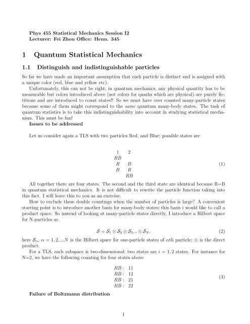
Phys 455 Statistical Mechanics Session I2
Lecturer: Fei Zhou Office: Henn. 345
1 Quantum Statistical Mechanics
1.1 Distinguish and indistinguishable particles
So far we have made an important assumption that each particle is distinct and is assigned with
a unique color (red, blue and yellow etc).
Unfortunately, this can not be right; in quantum mechanics, any physical quantity has to be
measurable but colors introduced above (not colors for quarks which are physical) are purely fictitious
and are introduced to count states!! So we must have over counted many-particle states
because some of them might correspond to the same quantum many-body states. The task of
quantum statistics is to take this indistinguishability into account in studying statistical mechanism.
This must be fun!
Issues to be addressed
Let us consider again a TLS with two particles Red, and Blue; possible states are
1 2
RB
R B
B R
RB
All together there are four states. The second and the third state are identical because R=B
in quantum statistical mechanics. It is not difficult to rewrite the particle function taking into
this fact. I will leave this to you as an exercise.
How to exclude these double countings when the number of particles is large? A convenient
starting point is to introduce another basis for many-body states; this basis i would like to call a
product space. So instead of looking at many-particle states directly, I introduce a Hilbert space
for N-particles as
S = S 1 ⊗ S 2 ⊗ S 3 ... ⊗ S N . (2)
here S α , α = 1, 2, ...N is the Hilbert space for one-particle states of αth particle; ⊗ is the direct
product.
For a TLS, each subspace is two-dimensional; two states are i = 1, 2 states. For instance for
N=2, we have the following counting for four states above
(1)
Failure of Boltzmann distribution
RB : 11
RB : 12
RB : 21
RB : 22
(3)
1

Once we use such a product space, we reproduce the partition function discussed in the previous
session in a different form
Z = ∑ ∑
.... ∑ exp(−βɛ i1 ) × exp(−βɛ i2 ).... exp(−βɛ iα )... × exp(−βɛ iN ). (4)
i1 i2 iN
Again α = 1, 2, ...N labels the color of particles and i labels the one-particle states running from
1 to n, n being the dimension of the one-particle Hilbert space. It reflects the democracy of
statistical mechanics.
This leads to the result we mentioned before
Z = Z 1 × Z 2 ... × Z α .... × Z N . (5)
So far we simply rewrite the known result of Boltzmann distribution.
If the dimension of one-particle Hilbert space n is much larger than the number of particles
involved for the study, Can one claim that the probability to find a one particle-state occupied by
two colored particles is negligible?
Exercise 1 Put forward arguments for or against this claim.
If under certain conditions that particles are unlikely to occupy the same state, the partition
function for indistinguishable particles is simply
Z = 1 N! Z 1 × Z 2 ... × Z α .... × Z N . (6)
Exercise 2 Show the prefactor N!.
In this limit,Botzmann distribution is an excellent approximation to reality. But what about
the opposite limit ?? How to deal with that limit?
Further demonstration
The previous claim is actually not correct. What one has to look at is the occupation of
particles at a given level.
n i = N exp( −ɛ i
kT ) 1 Z 1
. (7)
As an estimate one can show that this number if much less than one if
N ≪ D(kT ), (8)
where D(ɛ) is the number of one particle states at energies less than ɛ.
Take a box of particles. It is easily to show that the constraint indicates that
λ(T ) =
¯h
√
2mkT
≪ ( V N )1/d . (9)
d is the dimension of space. This means that the Boltzmann distribution is correct description of
the reality if the temperature of particles is sufficiently high. It breaks down at low temperatures,
which makes low temperature phenomena fascinating. Qualitatively, this is the limit where the
wave packet of particles of energy kT (the size of which is approximately λ) starts to overlap in
space.
2

1.2 Fermions and Bosons; Pauli exclusion principle
Since particles are indistinguishable, we have to decide the rule of games when two particles are
in the same one-particle state ɛ 1 . 1 Most natural choices one can make at this level are
Class A: No two particles can occupy the same state. (Pauli exclusion principle)
Class B: Two or more particles can occupy the same state.
Particles belonging to these two classes correspond to fermions and bosons respectively. We
will explore the consequencies of these two constraints on indistinguishable particles.
1.3 Fermi-Dirac statistics
A many-body state is represented by a series of bits or coordinates in the Fock space
And the Fock space is defined as a space
{N 1 , N 2 , ...N M }; N i = 0, 1. (10)
F = F 1 ⊗ ... ⊗ F M (11)
and F i is a space with two states (with different number of particles)
N i = 0, no particle occupying one-particle state i;
N i = 1, one particle occuping one-particle state i. (12)
Z =
∑
∑
N 1 =0,1 N 2 =0,1
...
∑
N n=0,1
ɛ 1 − µ
Ω(N 1 , N 2 , ...N n ) exp(−N 1
kT
) × ... × exp(−N ɛ n − µ
n ). (13)
kT
For indistinguishable particles, a many-body state is completely given by its coordinate in the
Fock space and Ω = 1.
Given this information one easily shows that
Z = Z 1 × ... × Z M ; Z i = 1 + exp(− ɛ i − µ
). (14)
kT
One can then show that the number of fermions at level i is
1
f F D =
1 + exp( ɛ (15)
i−µ
).
kT
This distribution function varies from 0 to 1.
Exercise 1 Show the Fermi-Dirac distribution function.
1 There might be more sophisticated classifications; furthermore there are so-call anyonic statistics differing from
the ones I am going to discuss. But I will not consider these possibilities because these are subjects under debate.
3

1.4 Bose-Einstein statistics
We can again write down the partition function for bosons
Z =
∞∑
∞∑
N 1 =0,... N 2 =0,...
...
∞∑
N M =0,...
ɛ 1 − µ
Ω(N 1 , N 2 , ...N n ) exp(−N 1
kT
) × ... × exp(−N M
Note that each summation is carried over all integers.
This partition function can be calculated directly and I find
ɛ M − µ
). (16)
kT
Z = Z 1 × ... × Z n ; Z i =
The average population of bosons at level i is
1
1 − exp(− ɛ (17)
i−µ
).
kT
f BE =
1
exp( ɛ i−µ
kT
) − 1.
(18)
It varies from zero to infinity. See nice discussions in the textbook, page 262-270. Especially figure
7.7.
Exercise 2 Derive f BE .
4