Computational Crystallography Newsletter (2010). 1, 4–11 - Phenix

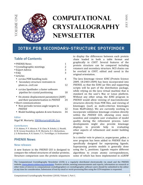
Volume ONE 

Computational 

Crystallography 

Newsletter  

JULY MMX 

Iotbx.PDB SECONDARY-STRUCTURE SPOTFINDER 

Table of Contents  

• PHENIX News        1  

• Crystallographic meetings      2  

• Expert Advice        3  

• FAQ            3  

• Articles  

• cctbx PDB handling tools     4  

•  Secondary structure restraints in  

phenix.refine        12  

• cctbx Spotfinder: a faster software  

 pipeline for crystal positioning    18  

• On atomic displacement parameters (ADP)  

and their parameterization in PHENIX  24  

• Short communications  

• Non‐periodic torsion angle targets in  

PHENIX          32  

• Model building updates & new features  34  

Editor  

Nigel W. Moriarty, NWMoriarty@LBL.Gov  

Contributors  

P. D. Adams, P. V. Afonine, V. B. Chen, N. Echols, J. J. Headd,  

R. W. Grosse‐Kunstleve, N. W. Moriarty, D. C. Richardson,  

J. S. Richardson, N. K. Sauter, T. C. Terwilliger, A. Urzhumtsev  

PHENIX News  

New releases  

A  new  feature  in  the  PHENIX  GUI  is  designed  to  

compare the refined structures of similar proteins.  

Structure comparison uses the protein sequences  

to  display  the  differences  between  each  protein  

chain  loaded  in  both  a  table  format  and  

graphically  in  COOT.  Several  features  of  the  

protein  structure  can  be  compared  including  

rotamers and secondary structure. NCS chains can  

be  overlaid  in  COOT,  edited  and  saved  in  the  

original orientation.  

The  Java  kinemage  viewer  KiNG  (Protein  Science  

2009,  18:2403‐2409)  has  been  incorporated  into  

PHENIX, so that the KiNG jar files and supporting  

scripts  will  be  part  of  the  distribution  package,  

while  relying  on  the  Java  virtual  machine  that  is  

standard  on  the  user's  Mac  or  Linux  platform.  

Without  any  other  setup,  the  KiNG  program  in  

PHENIX  would  allow  viewing  of  macromolecular  

structures directly from PDB files, and viewing of  

kinemages  (such  as  multi‐criterion  kinemages  

from  MolProbity).  We  are  currently  working  to  

incorporate validation kinemage creation directly  

within  the  PHENIX  GUI,  allowing  even  more  

seamless  and  complete  user  evaluation  of  model  

quality during  the  refinement  process.  Later  

developments  might  also  provide  kinemage  

displays  to  provide  help  in  evaluating  

other  aspects  of  refinement  and  model  building  

progress.  

In a similar vein to phenix.superpose_pdbs, a  

new  program  has  been  added  to  PHENIX  that  is  

specifically  designed  for  superposing  ligands.  

Superposing  protein  models  is  generally  done  

using  the  C α   positions.  Ligands  require  different  

algorithms  to  create  atomic  correspondences,  

some  of  which  has  been  implemented  in  eLBOW  

The  Computational  Crystallography  Newsletter  (CCN)  is  a  regularly  distributed  electronically  via  email  and  the  PHENIX  

website, www.phenix‐online.org/newsletter. Feature articles, meeting announcements and reports, information on research or  

other items of interest to computational crystallographers or crystallographic software users should be submitted to the editor  

at any time for consideration. Submission of text by email or word‐processing files using the CCN templates is requested.  

  1  

Computational Crystallography Newsletter (2010). Volume 1, Part 1. 

  

(Moriarty  et.  al.,  Acta  Cryst.,  D65,  2009,  1074– 

1080).  eLBOW’s  methods  including  graph  

matching  are  used  to  match  the  atoms  from  a  

single  molecule  or  group  of  residues  to  another  

single  molecule.  The  resulting  correspondences  

can be used in several ways. The molecules can be  

aligned  using  the  least‐squares  residual  of  the  

distances  between  matched  atoms;  the  exact  

position  of  the  corresponding  atoms  can  be  

transferred;  or  the  PDB  attributes  such  as  atom  

name and residue name can be transferred. A file  

containing  a  protein  and  ligand  can  be  used  as  

input  and  multiple  instances  of  the  ligand  can  be  

handled. The program can be accessed by running  

phenix.superpose_ligands.  

A  tool  developed  especially  for  our  industrial  

consortium  members  and  designed  to  decrease  

the  time  to  fit  a  ligand  by  using  a  previously  

positioned  ligand  in  the  same  or  similar  protein  

model  has  been  added  to PHENIX.  Guided  Ligand  

Replacement  (GLR)  matches  the  protein  models,  

determines the location of the fit ligand, performs  

an  atomic  match  of  the  ligands  and  inserts  the  

overlaid  ligand  into  the  apo  protein  model.    As  a  

final step, a real‐space refinement is performed on  

the  ligand  and  the  surrounding  protein.  GLR  

attempts  to  match  all  instances  of  the  guiding  

ligand in the asymmetric unit.  

New features  

RESOLVE in PHENIX is now entirely C++ code. This  

allows the use of the cctbx routines in RESOLVE  

and  speeds  up  RESOLVE  model‐building  by  a  

factor of  nearly  two.   It  also  allows  caching  of  

resolve libraries, further speeding up RESOLVE in  

PHENIX.  

Ligand  fitting  in  PHENIX  now  incorporates  realspace refinement, yielding greatly improved fits of  

ligand to density.  

Loop  libraries  have  been  created  for  rapid  fitting  

of short loops with phenix.fit_loops.  

The ligand geometry restraints editor, REEL, has a  

new feature that allows searching of the Chemical  

Components  Dictionary  available  at  

http://www.wwpdb.org/ccd.html  and  also  

distributed  with  PHENIX.  The  user  can  search  

using  various  ligand  attributes  including  name  

and chemical formula.  The results can be viewed  

in the molecular viewing window.  

Current PHENIX development  

Work  is  currently  underway  to  improve  the  

support  for  carbohydrates  in  macromolecular  

models.  The  GlycoCT  format  (Herget  et  al.,  

Carbohydr. Res., 2008, 343:2162‐2171) which can  

specify a carbohydrate sequence has been chosen  

as  the  base  format  for  file  based  input.  Other  

formats  will  be  supported.  A  GUI  input  is  also  

being developed as well as tools to handle models  

already  containing  the  carbohydrates.  It  is  

expected  that  ligand  fitting  will  be  expanded  to  

improve  the  fitting  of  carbohydrates  focusing  on  

the  saccharide  chains  that  commonly  occur  in  

protein models.  Branching will be supported from  

the inception.  

Crystallographic meetings and  

workshops  

2010  Australasian  Crystallography  School,  17‐24  

July, 2010  

The  2010  Australasian  Crystallography  School  is  

being  held  at  the  University  of  Queensland,  

Brisbane,  Australia  from  the  17 th   to  the  24 th   of  

July.  Pavel  Afonine  will  be  teaching  a  module  on  

macro‐molecular refinement.  

GRC – Diffraction Method in Crystallography, 18‐23  

July 2010   

Several  of  the  PHENIX  developers  will  be  

attending  the  Gordon  Conference  entitled  

“Diffraction  Methods  in  Crystallography”  to  be  

held  at  Bates  College,  Lewiston,  Maine  from  the  

18 th   to  the  23 rd   of  July.    There  will  be  posters  on  

the  various  aspects  of  PHENIX  including  the  

graphical  user  interface,  validation  and  ligands.   

Drop by during the poster sessions to speak to the  

developers.  

ACA – 2010 Annual Meeting, 24‐29 July, 2010  

The  annual  meeting  of  the  American  

Crystallographic  Association  will  be  held  in  

Chicago, Illinois from the 24 th  to the 29 th  of July.  

22 nd  PHENIX Workshop, 11‐13 October, 2010  

The  semi‐annual  PHENIX  workshop  is  being  held  

in Cambridge, England from the 11 th  to the 13 th  of  

October.  Developers  will  be  presenting  the  latest  

programs  and  feature  releases  on  Monday  the  

  2  


  

11 th . All interested parties in the area are invited  

to attend the Monday sessions.  

5 th  PHENIX User’s Workshop, 14 October, 2010  

Following  the  PHENIX  Workshop  in  Cambridge  

U.K., a user’s workshop will provide teaching and  

hands‐on  experience  with  PHENIX  for  the  novice  

and expert.  

Paris Workshop, 15 October, 2010  

A  contingent  of  PHENIX  developers  will  be  at  

Institut  Pasteur,  Paris,  France  on  the  15 th   of  

October to participate in a workshop for the local  

users.  The  workshop  is  being  organized  by  

Claudine  Mayer  and  Deshmukh  Gopaul  and  is  

funded  by  the  "Groupe  Thematique  Biologie"  of  

the French Crystallography Association.  

Expert advice  

Geometry restraint ESD  

Many  users  enquire  about  the  details  of  the  

geometry  restraints  used  in  macromolecular  

refinement  programs.  Refmac,  COOT  and  PHENIX  

use a CIF format; an example of the restraints for  

water appears at right.  

Much  of  the  information  in  the  file  is  

straightforward  including  atom  names,  elements  

and  Cartesian  coordinates.  Even  the  bonding  

information  is  mostly  transparent.  The  atoms  

involved,  the  type  of  bond  and  the  ideal  bond  

lengths  are  easily  discerned.  The  last  number  on  

the line, however, is not so simple. The ESD is an  

Estimated  Standard  Deviation  that  allows  a  

refinement  program  to  estimate  the  gradients  of  

the  force  on  the  two  atoms  in  the  bond  using  a  

parabola. The units of the ESD are the same as the  

ideal  value  so  for  bond  lengths  the  unit  is  

Ångstrom.  The  larger  the  ESD  value,  the  more  

flexible  the  restraint  will  be  in  the  refinement.  

Conversely, reducing the number will restrain the  

internal  coordinate  to  remain  closer  to  the  ideal  

value.  

There is a limit to the amount one can reduce the  

ESD of a restraint. In the extreme, setting the ESD  

value  to  zero  will  remove  the  restraint  from  the  

refinement. Also, reducing the ESD to a value that  

is orders of magnitude smaller than the other ESD  

values  in  the  same  class  will  greatly  reduce  the  

data_comp_list 

loop_ 

_chem_comp.id 

_chem_comp.three_letter_code 

_chem_comp.name 

_chem_comp.group 

_chem_comp.number_atoms_all 

_chem_comp.number_atoms_nh 

_chem_comp.desc_level 

HOH HOH 'water ' ligand 3 1 . 

data_comp_HOH 

loop_ 

_chem_comp_atom.comp_id 

_chem_comp_atom.atom_id 

_chem_comp_atom.type_symbol 

_chem_comp_atom.type_energy 

_chem_comp_atom.partial_charge 

_chem_comp_atom.x 

_chem_comp_atom.y 

_chem_comp_atom.z 

HOH O O OH2 . -0.2400 0.0000 -0.3394 

HOH H1 H HOH2 . 0.8400 0.0000 -0.3394 

HOH H2 H HOH2 . -0.6000 0.0000 0.6788 

loop_ 

_chem_comp_bond.comp_id 

_chem_comp_bond.atom_id_1 

_chem_comp_bond.atom_id_2 

_chem_comp_bond.type 

_chem_comp_bond.value_dist 

_chem_comp_bond.value_dist_esd 

HOH H1 O single 1.080 0.020 

HOH H2 O single 1.080 0.020 

loop_ 

_chem_comp_angle.comp_id 

_chem_comp_angle.atom_id_1 



_chem_comp_angle.value_angle 

_chem_comp_angle.value_angle_esd 

HOH H2 O H1 109.47 3.000 

weight of the other restraints relative to the highly  

restrained  value  and  may  even  adversely  affect  

the weight of the x‐ray term.  

Generally,  it  is  best  to  have  the  ESD  values  

approximately the same as the expected accuracy  

of the experiment. In the case of the bond lengths,  

an  ESD  of  0.01  Ångstrom  could  be  considered  a  

reasonable lower bound. An angle ESD of about 1  

degree  and  torsion  ESD  of  5  degrees  are  also  

reasonable as a lower limit.  

FAQ  

How do I create restraints for my ligand in PHENIX?  

There  are  a  number  of  ways.    If  you  know  the  

ligand  code  corresponding  to  the  ligand  in  the  

PDB databases such as the Chemical Components,  

then you can use eLBOW thus:  

phenix.elbow --chemical-component=ATP 

The  resulting  files,  ATP.pdb  and  ATP.cif,  will  

have the data such as atom names consistent with  

the Chemical Components database.  

  3  


  

ARTICLES 

 cctbx PDB handling tools  

Ralf W. Grosse‐Kunstleve a  and Paul D. Adams a,b   

aLawrence Berkeley National Laboratory, Berkeley, CA 94720  

bDepartment of Bioengineering, University of California at Berkeley, Berkeley, CA 94720  

Correspondence email: RWGrosse‐Kunstleve@LBL.Gov  

Introduction  

The PDB format is the predominant working format for atomic parameters (coordinates, occupancies,  

displacement parameters, etc.) in macromolecular crystallography. Many small‐molecule programs also  

support this format. The PDB format specifications are available at http://www.pdb.org/. Technically,  

the format is very simple, therefore a vast number of parsers exist in scientific packages. This article is  

about  the  PDB  handling  tools  included  in  the  Computational  Crystallography  Toolbox  (cctbx,  

http://cctbx.sourceforge.net/), the open‐source component of the PHENIX project (http://www.phenixonline.org/).  

The  evolution  of  the  cctbx  PDB  handling  tools  has  gone  through  three  main  stages  spread  out  over  

several years. A simple parser implemented in Python has been available for a long time. In many cases  

Python's runtime performance is sufficient for interactive processing of PDB files, but can be limiting for  

large files, or for repeatedly traversing the entire PDB database. This has prompted us to implement a  

fast  C++  parser  that  is  described  in  Grosse‐Kunstleve  et  al.  (2006).  However,  initially  the  fast  cctbx  

PDB handling tools only supported "read‐only" access. Writing of PDB files was supported only at a very  

basic level. This shortcoming has been removed and the current cctbx version provides comprehensive  

tools for reading, manipulating, and writing PDB files. These tools are available from both Python and  

C++, under the iotbx.pdb module.  

This article presents an overview of the main types in the iotbx.pdb module, considerations that lead  

to  the  design,  and  related  important  nomenclature.  It  is  not  a  tutorial  for  using  the  iotbx.pdb  

facilities.  For  this,  refer  to  http://cctbx.sourceforge.net/sbgrid2008/tutorial.html.  See  also  

http://cci.lbl.gov/hybrid_36/ which describes iotbx.pdb facilities for handling very large models.  

Real‐world PDB files  

The simplicity of the PDB format is only superficial and, in the general case, stops after the initial parsing  

level.  The  structure  of  the  PDB  file  implies  a  hierarchy  of  objects.  A  first  approximation  is  this  

hierarchical view is:  

model 

chain 

residue 

atom 

This  is  only  an  approximation  because  of  a  feature  that  is  easily  overlooked  at  first:  the  "altloc"  

(official  PDB  nomenclature)  column  17  of  PDB  ATOM  records,  specifying  "alternative  location"  

identifiers for atoms in alternative conformations. As it turned out, about 90% of the development time  

invested  into  iotbx.pdb  was  in  some  form  related  to  alternative  conformations.  Our  goal  was  to  

provide  robust  tools  that  work  even  for  the  most  unusual  (but  valid)  cases,  since  this  is  a  vital  

characteristic  of  any  automated  system.  The  main  difficulties  encountered  while  pursuing  this  goal  

were:  

• Chains with conformers that have different sequences  

• Chains with duplicate resseq+icode (residue sequence number + insertion code)  

• Conformers interleaved or separated  

  Computational Crystallography Newsletter (2010). 1, 4–11  

4 

  

ARTICLES 

These difficulties are best illustrated with examples. An old version of PDB entry 2IZQ (from Aug 2008)  

includes a chain with conformers that have different sequences, the residue with resseq 11 in chain A,  

atoms 220 through 283:  

HEADER ANTIBIOTIC 26-JUL-06 2IZQ 

ATOM 220 N ATRP A 11 20.498 12.832 34.558 0.50 6.03 N 

................ATRP A 11 ................................................... 

ATOM 243 HH2ATRP A 11 15.522 9.077 38.323 0.50 10.40 H 

ATOM 244 N CPHE A 11 20.226 13.044 34.556 0.15 6.35 N 

................CPHE A 11 ................................................... 

ATOM 254 CZ CPHE A 11 16.789 9.396 34.594 0.15 10.98 C 

ATOM 255 N BTYR A 11 20.553 12.751 34.549 0.35 5.21 N 

................BTYR A 11 ................................................... 

ATOM 261 CD1BTYR A 11 18.548 10.134 34.268 0.35 9.45 C 

ATOM 262 HB2CPHE A 11 21.221 10.536 34.146 0.15 7.21 H 

ATOM 263 CD2BTYR A 11 18.463 10.012 36.681 0.35 9.08 C 

ATOM 264 HB3CPHE A 11 21.198 10.093 35.647 0.15 7.21 H 

ATOM 265 CE1BTYR A 11 17.195 9.960 34.223 0.35 10.76 C 

ATOM 266 HD1CPHE A 11 19.394 9.937 32.837 0.15 10.53 H 

ATOM 267 CE2BTYR A 11 17.100 9.826 36.693 0.35 11.29 C 

ATOM 268 HD2CPHE A 11 18.873 10.410 36.828 0.15 9.24 H 

ATOM 269 CZ BTYR A 11 16.546 9.812 35.432 0.35 11.90 C 

ATOM 270 HE1CPHE A 11 17.206 9.172 32.650 0.15 12.52 H 

ATOM 271 OH BTYR A 11 15.178 9.650 35.313 0.35 19.29 O 

ATOM 272 HE2CPHE A 11 16.661 9.708 36.588 0.15 11.13 H 

ATOM 273 HZ CPHE A 11 15.908 9.110 34.509 0.15 13.18 H 

ATOM 274 H BTYR A 11 20.634 12.539 33.720 0.35 6.25 H 

................BTYR A 11 ................................................... 

ATOM 282 HH BTYR A 11 14.978 9.587 34.520 0.35 28.94 H 

  

The original atom numbering does not have gaps. Here we have omitted blocks of atoms with constant  

resname and resseq+icode to save space.  

As of Jun 8 2010, there are 74 files with mixed residue names in the PDB, i.e. only about 0.1% of the files.  

However, these files are perfectly valid and a PDB processing library is suitable as a component of an  

automated system only if it handles them sensibly.  

An  old  version  of  PDB  entry  1ZEH  (Aug  2008)  includes  a  chain  with  consecutive  duplicate  

resseq+icode, atoms 878 through 894:  

HEADER HORMONE 01-MAY-98 1ZEH 

HETATM 878 C1 ACRS 5 12.880 14.021 1.197 0.50 33.23 C 

HETATM 879 C1 BCRS 5 12.880 14.007 1.210 0.50 34.27 C 

................ACRS 5 ................................................... 

HETATM 892 O1 ACRS 5 11.973 14.116 2.233 0.50 34.24 O 

HETATM 893 O1 BCRS 5 11.973 14.107 2.248 0.50 35.28 O 

HETATM 894 O HOH 5 -0.924 19.122 -8.629 1.00 11.73 O 

HETATM 895 O HOH 6 -19.752 11.918 3.524 1.00 13.44 O 

HETATM 896 O HOH 7 -1.169 17.936 -6.103 1.00 12.89 O 

  

To  a  human  inspecting  the  old  1ZEH  entry,  it  is  of  course  immediately  obvious  that  the  water  with  

resseq 5 is not related to the previous residue with resseq 5. However, arriving at this conclusion  

with an automatic procedure is not entirely straightforward. The human brings in the knowledge that  

water  atoms  without  hydrogen  are  not  covalently  connected  to  other  atoms.  This  is  very  detailed,  

specialized  knowledge.  Introducing  such  heuristics  into  an  automatic  procedure  is  likely  to  lead  to  

surprises in some situations and is best avoided, if possible.  


5 

  

ARTICLES 

In  the  PDB  archive,  alternative  conformers  of  a  residue  always  appear  consecutively.  However,  as  

mentioned in the introduction, the PDB format is also the predominant working format. Some programs  

produce files with conformers separated in this way (this file was provided to us by a user):  

ATOM 1716 N ALEU 190 28.628 4.549 20.230 0.70 3.78 N 

ATOM 1717 CA ALEU 190 27.606 5.007 19.274 0.70 3.71 C 

ATOM 1718 CB ALEU 190 26.715 3.852 18.800 0.70 4.15 C 

ATOM 1719 CG ALEU 190 25.758 4.277 17.672 0.70 4.34 C 

ATOM 1829 N BLEU 190 28.428 4.746 20.343 0.30 5.13 N 

ATOM 1830 CA BLEU 190 27.378 5.229 19.418 0.30 4.89 C 

ATOM 1831 CB BLEU 190 26.539 4.062 18.892 0.30 4.88 C 

ATOM 1832 CG BLEU 190 25.427 4.359 17.878 0.30 5.95 C 

ATOM 1724 N ATHR 191 27.350 7.274 20.124 0.70 3.35 N 

ATOM 1725 CA ATHR 191 26.814 8.243 21.048 0.70 3.27 C 

ATOM 1726 CB ATHR 191 27.925 9.229 21.468 0.70 3.73 C 

ATOM 1727 OG1ATHR 191 28.519 9.718 20.259 0.70 5.22 O 

ATOM 1728 CG2ATHR 191 28.924 8.567 22.345 0.70 4.21 C 

ATOM 1729 C ATHR 191 25.587 8.983 20.559 0.70 3.53 C 

ATOM 1730 O ATHR 191 24.872 9.566 21.383 0.70 3.93 O 

... residues 191 through 203 not shown 

ATOM 1828 O AGLY 203 8.948 14.861 23.401 0.70 5.84 O 

ATOM 1833 CD1BLEU 190 26.014 4.711 16.521 0.30 6.21 C 

ATOM 1835 C BLEU 190 26.506 6.219 20.135 0.30 4.99 C 

ATOM 1836 O BLEU 190 25.418 5.939 20.669 0.30 5.91 O 

ATOM 1721 CD2ALEU 190 24.674 3.225 17.536 0.70 5.31 C 

ATOM 1722 C ALEU 190 26.781 6.055 20.023 0.70 3.36 C 

ATOM 1723 O ALEU 190 25.693 5.796 20.563 0.70 3.68 O 

ATOM 8722 C DLEU 190 26.781 6.055 20.023 0.70 3.36 C 

ATOM 8723 O DLEU 190 25.693 5.796 20.563 0.70 3.68 O 

ATOM 9722 C CLEU 190 26.781 6.055 20.023 0.70 3.36 C 

ATOM 9723 O CLEU 190 25.693 5.796 20.563 0.70 3.68 O 

In  this  file,  conformers  A  and  B  of  residue  190  appear  consecutively,  but  conformers  C  and  D  appear  

only after conformers A and B of all residues 191 through 203. While this is not the most intuitive way of  

ordering the residues in a file, it is still considered valid because the original intention is clear. Since it  

was our goal to develop a comprehensive library suitable for automatically processing files produced by  

any popular program, we found it important to correctly handle non‐consecutive conformers.   

iotbx.pdb.hierarchy  

When developing the procedure capable of handling the variety of real‐world situations shown above,  

we strived to keep the underlying rule‐set as simple as possible and to avoid highly specific heuristics  

(e.g. "water is never covalently bound"). Complex rules imply complex implementations, are difficult to  

explain  and  understand,  tend  to  lead  to  surprises,  and  are  therefore  likely  to  be  rejected  by  the  

community.  With  this  and  the  real‐world  situations  in  mind,  we  arrived  at  the  following  primary  

organization of the PDB hierarchy:  

Primary PDB hierarchy: 

model(s) 

id 

chain(s) 

id 

residue_group(s) 

resseq 

icode 

atom_group(s) 

resname 

altloc 

atom(s) 


6 

  

ARTICLES 

  

In this presentation the "(s)" indicates a list of objects of the given type. i.e. a hierarchy contains a list of  

models, each model has an "id" (a simple string) and holds a list of chains, etc.   

Comparing with the "first approximation hierarchy" above, the residue type is replaced with two new  

types:    residue_group  and  atom_group.  These  types  had  to  be  introduced  to  cover  all  the  realworld cases shown above. The residue_group and atom_group types are new and unusual. Before  

we go into the details of these types, it will be helpful to consider the bigger picture by introducing the  

alternative secondary view of the PDB hierarchy:  

Secondary view of PDB hierarchy: 

model(s) 

id 

chain(s) 

id 

conformer(s) 

altloc 

residue(s) 

resname 

resseq 

icode 

atom(s) 

  

This organization is probably more intuitive at first. The first two levels (model, chain) are exactly the  

same  as  in  the  primary  hierarchy.  Each  chain  holds  a  list  of  conformer  objects,  which  are  

characterized  by  the  altloc  character  from  column  17  in  the  PDB  ATOM  records.  A  conformer  is  

understood  to  be  a    complete  copy    of  a  chain,  but  usually  two  conformers  share  some  or  even  most  

atoms.  A residue is characterized by a unique resname and the resseq+icode.  

The  secondary  view  of  the  hierarchy  evolved  in  the  context  of  generating  geometry  restraints  for  

refinement (e.g. bond, angle, and dihedral restraints), where this organization is most useful. It is also  

the  organization  introduced  in  Grosse‐Kunstleve  et  al.  (2006),  where  it  was  actually  the  primary  

organization.  While  working  with  the  conformer‐residue  organization,  we  found  that  it  is  difficult  to  

manipulate  a  hierarchy  (e.g.  add  or  delete  atoms)  in  obvious  ways.  Finally,  while  developing  the  

automatic  generation  of  constrained  occupancy  groups  for  alternative  conformations,  the  conformerresidue organization proved to be unworkable. The main difficulty is that the relative order of residues  

with alternative conformations is lost in the conformer‐residue organization; it is only given indirectly  

by interleaved residues with shared atoms ‐‐ if they exist. As convenient as the conformer-residue  

organization is for the generation of restraints, it is a hindrance for other purposes.   

The names for the new types in the primary hierarchy were chosen not to collide with the secondary  

view. We could have used "conformer" and "residue" again, just reversed, but there would be the  

big surprise that one residue has different resnames. To send the signal "this is not what you usually  

think of as a residue", we decided to use residue_group as the type name. A residue group holds a  

list  of  atom_group  objects.  All  atoms  in  an  atom  group  have  the  same  resname  and  altloc.  

Therefore  "resname_altloc_group"  would  have  been  another  plausible  name,  but  we  favored  

atom_group since it is more concise and better conveys what is the main content.  

Detection of residue groups and atom groups  

When  constructing  the  primary  hierarchy  given  a  PDB  file,  the  processing  algorithm  has  to  detect  

models, chains, residue groups, atom groups and atoms. Most steps are fairly straightforward, but none  

of the steps is actually completely trivial. For example, what to do if TER or ENDMDL cards are missing?  

What if residue sequence numbers are not consecutive? The ribosome community widely uses segid  

instead of chain id (even though the segid column is officially deprecated by the PDB). What if a file  


7 

  

ARTICLES 

contains both chain id and segid? Documenting all our answers in full detail is beyond the scope of  

this  article  (and  would  be  more  distracting  than  helpful  anyway  because  the  source  code  is  openly  

available). Therefore we concentrate on the  most  important  rules  for  the  detection  of  residue  groups  

and atom groups.  

Then central conflict we had to resolve was:  

• In order to handle non‐consecutive conformers, we have to use the resseq+icode to find and  

group related residues.  

• However, we cannot use the resseq+icode alone as a guide, because we also want to handle  

chains with duplicate resseq+icode (consecutive or non‐consecutive).  

This lead to a two stage procedure. In the first stage:  

• A residue group is given by a block of consecutive ATOM or HETATM records with identical  

resseq+icode columns (SIGATM, ANISOU, and SIGUIJ records may be interleaved), e.g.  

ATOM 234 H ATRP A 11 20.540 12.567 33.741 0.50 7.24 H 

ATOM 235 HA ATRP A 11 20.771 12.306 36.485 0.50 6.28 H 

ATOM 244 N CPHE A 11 20.226 13.044 34.556 0.15 6.35 N 

ATOM 245 CA CPHE A 11 20.950 12.135 35.430 0.15 5.92 C 

  

However, there is an important pre‐condition:  

• Unless a sub‐block of ATOM records with identical resname+resseq+icode columns  

contains a main‐conformer atom (almost "blank altloc"), e.g.  

HEADER ANTIBIOTIC RESISTANCE 07-MAY-97 1AJQ 

CRYST1 52.120 65.080 76.300 100.20 111.44 105.81 P 1 1 

HETATM 6097 CA CA 1 5.676 34.115 52.446 1.00 18.50 CA 

HETATM 6100 C2 SPA 1 11.860 36.159 33.853 1.00 14.30 C 

HETATM 6107 C6 SPA 1 13.085 36.522 34.644 1.00 17.34 C 

In this case the sub‐block is assigned to a separate residue group.  

Within each residue group, all atoms are grouped by altloc+resname and assigned to atom groups.  

The order of the atoms in a residue group does not affect the assignment to atom groups.  

After all atom records are assigned to residue groups and atom groups,  

• residue groups with identical resseq+icode  

• that do not contain main‐conformer atoms  

are  merged  in  the  second  processing  stage.  While  two  residue  groups  are  merged,  atom  groups  with  

identical altloc+resname from the two sources are also merged.  

Note  that  the  grouping  steps  in  this  process  may  change  the  order  of  the  atoms.  However,  our  

implementation  preserves  the  relative  order  of  the  atoms  as  much  as  possible.  I.e.  in  the  hierarchy,  

resseq+icode appear in the original "first seen" order, and similarly for altloc+resname within a  

residue group.  

Construction of secondary view of hierarchy  

The  secondary  view  of  the  hierarchy  is  constructed  trivially  from  the  primary  hierarchy  objects.  For  

each  chain,  the  complete  list  of  altloc  characters  is  determined  in  a  first  pass.  In  a  second  pass,  a  

conformer  object  is  created  for  each  altloc,  and  a  second  loop  over  the  chain  assigns  the  atoms  to  

each  conformer.  Main‐conformer  atoms  are  assigned  to  all  conformers,  atoms  in  alternative  


8 

  

ARTICLES 

conformations  only  to  the  corresponding  conformer.  Because  of  the  difficulties  alluded  to  earlier,  the  

conformer  and  residue  objects  in  the  secondary  view  are  "read‐only".  I.e.  all  manipulations  such  as  

addition  or  removal  of  residues,  have  to  be  performed  on  the  primary  hierarchy.  Re‐constructing  the  

secondary view after the primary hierarchy has been changed is very fast (fractions of seconds even for  

the largest files, e.g. 0.22 s for PDB entry 1HTQ with almost one million atoms).  

The  iotbx/examples/pdb_hierarchy.py  script  shows  how  to  construct  the  primary  hierarchy  

from a PDB file, and how to obtain the secondary view.  

Nomenclature related to alternative conformations  

The  iotbx.pdb  module  uses  the  following  nomenclature  to  describe  various  aspects  of  alternative  

conformations:  

• Main conf. atom : an atom with  

o a blank altloc character  

o and no other atom with the same name+resname (but different altloc) in the residue  

group. This second condition is needed for cases like this:  

HEADER HYDROLASE 12-MAR-04 1SO7 

ATOM 2460 CG1 VAL A 325 -23.284 97.713 15.815 0.66 21.74 C 

ATOM 2461 CG1AVAL A 325 -23.010 97.616 18.295 0.66 22.88 C 

ATOM 2462 CG2BVAL A 325 -24.819 96.373 17.146 0.66 22.57 C 

• Alt. conf. atom : not main conf.  

• Conformer : a complete chain with main conf. atoms and alt. conf. atoms with a specific altloc.  

  

Note for completeness: it is also possible to obtain conformers of an individual residue group.  

However, conceptually this is best viewed as a shortcut for first obtaining the conformers of a  

chain, and then finding the residue of interest in each conformer, ignoring all other residues.  

  

• Residue : complete residue in a conformer with main conf. atoms and alt. conf. atoms.  

Residues are classified as follows:  

• pure main conf. : all main conf. atoms  

• pure alt. conf. : all alt. conf. atoms  

• proper alt. conf. : both main conf. atoms and alt. conf atoms, all alt conf. atoms have a non‐blank  

altloc column  

• improper alt. conf. : both main conf. atoms and alt. conf atoms, one or more alt conf. atoms have  

a blank altloc column (as shown in the 1SO7 fragment above).  

Errors and warnings  

The tools in iotbx.pdb are designed to be as tolerant as reasonably possible when processing input  

PDB files. E.g., as of Jun 8 2010, all 65802 files in the PDB archive can be processed without generating  

exceptions.  However,  to  assist  users  and  developers  in  creating  PDB  files  without  ambiguities,  the  

hierarchy object provides methods for flagging likely problems as errors and warnings. It is up to the  

application how to react to the diagnostics.  

The phenix.pdb.hierarchy command can be used to quickly obtain a summary of the hierarchy in  

a PDB file and some diagnostics. This example command highlights all main features:  

phenix.pdb.hierarchy pdb1jxw.ent.gz 


9 

  

ARTICLES 

Output:  

  

  

file pdb1jxw.ent.gz 

total number of: 

models: 1 

chains: 2 

alt. conf.: 5 

residues: 49 

atoms: 786 

anisou: 0 

number of atom element+charge types: 5 

histogram of atom element+charge frequency: 

" H " 383 

" C " 261 

" O " 77 

" N " 59 

" S " 6 

residue name classes: 

"common_amino_acid" 48 

"other" 1 

number of chain ids: 2 

histogram of chain id frequency: 

" " 1 

"A" 1 

number of alt. conf. ids: 3 

histogram of alt. conf. id frequency: 

"A" 2 

"B" 2 

"C" 1 

residue alt. conf. situations: 

pure main conf.: 32 

pure alt. conf.: 3 

proper alt. conf.: 14 

improper alt. conf.: 0 

chains with mix of proper and improper alt. conf.: 0 

number of residue names: 16 

histogram of residue name frequency: 

"CYS" 6 

"THR" 6 

"ALA" 5 

"ILE" 5 

"PRO" 5 

"GLY" 4 

"ASN" 3 

"SER" 3 

"ARG" 2 

"LEU" 2 

"TYR" 2 

"VAL" 2 

"ASP" 1 

"EOH" 1 other 

"GLU" 1 

"PHE" 1 

### WARNING: consecutive residue_groups with same resid ### 

number of consecutive residue groups with same resid: 2 

residue group: 

"ATOM 378 N PRO A 22 .*. N " 

... 12 atoms not shown 

"ATOM 391 HD3APRO A 22 .*. H " 

next residue group: 

"ATOM 392 CB BSER A 22 .*. C " 


"ATOM 399 HB3CSER A 22 .*. H " 

------------------------------------------ 

residue group: 

"ATOM 432 N LEU A 25 .*. N " 


"ATOM 439 CD1CLEU A 25 .*. C " 

next residue group: 

"ATOM 452 CG1BILE A 25 .*. C " 


"ATOM 466 HD13CILE A 25 .*. H " 


10 

  

ARTICLES 

The diagnostics are mainly intended for PDB working files, but we have tested the iotbx.pdb  module  

by processing the entire PDB archive. (This took about 3700 CPU seconds, but using 40 CPUs the last job  

finished after only 277 seconds. Disk and network I/O is rate‐limiting in this case, not the performance  

of the PDB handling library.) The results are summarized in the following table:  

Total number of .ent files: 65802 (2010 Jun 8) 

56873 WARNING: duplicate chain id 

3 WARNING: consecutive residue_groups with same resid 

2 ERROR: duplicate atom labels 

1 ERROR: improper alt. conf. 

0 ERROR: duplicate model id 

0 ERROR: residue group with multiple resnames using same altloc 

About 86% of the PDB entries re‐use the same chain id for multiple chains (which are either separated  

by other chains or TER cards). In many cases, the re‐used chain id is the blank character, which is clearly  

a  minor  issue.  However,  we  flag  this  situation  to  assist  people  in  producing  new  PDB  files  with  

unambiguous chain ids.  

The  next  item  in  the  list,  "consecutive  residue_groups  with  same  resid"  (where  

resid=resseq+icode),  was  mentioned  before.  This  situation  is  best  avoided  to  minimize  the  

chances of mis‐interpreting the PDB files.  

 "duplicate  atom  labels"  pose  a  serious  practical  problem  (therefore  flagged  as  "ERROR")  since  it  is  

impossible to uniquely select atoms with duplicate labels, for example via an atom selection syntax as  

used  in  many  programs  (CNS,  PyMOL,  PHENIX,  VMD,  etc.)  or  via  PDB  records  in  the  connectivity  

annotation section (LINK, SSBOND, CISPEP). Atom serial numbers are not suitable for this purpose since  

many programs do not preserve them.  

Only one PDB entry (1JRT) includes "improper alt. conf." as introduced in the previous section.  

There are no PDB entries with two other potential problems diagnosed by the iotbx.pdb module. MODEL  

ids  are  unique  throughout  the  PDB  archive  (as  an  aside:  and  all  MODEL  records  have  a  matching  

ENDMDL  record).  Finally,  in  all  74  files  with  mixed  residue  names  (i.e.  conformers  with  different  

sequences), there is exactly one residue name for a given altloc.  

 Acknowledgments  

We  gratefully  acknowledge  the  financial  support  of  NIH/NIGMS  under  grant  number  P01GM063210.  

Our  work  was  supported  in  part  by  the  US  Department  of  Energy  under  Contract  No.  DE‐AC02‐ 

05CH11231.  

 References  

Grosse‐Kunstleve,  R.W.,  Zwart,  P.H.,  Afonine,  P.V.,  Ioerger,  T.R.,  Adams,  P.D.  (2006).  Newsletter  of  the  

IUCr Commission on Crystallographic Computing, 7, 92‐105.  

  


11 

  

ARTICLES 

Secondary structure restraints in phenix.refine  

Nathaniel Echols a , Jeffrey J. Headd a , Pavel Afonine a , and Paul D. Adams a,b   



Correspondence email: NEchols@LBL.Gov   


We  have  implemented  simple,  automatic  restraints  for  common  secondary  structure  elements  in  

proteins  and  nucleic  acids,  which  can  help  reduce  over‐fitting  at  low‐to‐moderate  resolution  and  

preserve the secondary structure geometry that can be distorted due to the low resolution.  Internally,  

these are simply distance restraints between hydrogen‐bonding atoms in helices, sheets, or nucleic acid  

base  pairs,  with  or  without  explicit  hydrogens.    The  current  method  has  the  advantage  of  being  fast,  

easily reduced to relatively simple input parameters, and useful for improving poor‐quality regions of  

structure where the bonding may not be automatically recognized.  

General description and syntax  

A  new  command  for  identifying  secondary  structure  and  generating  the  necessary  parameters,  

phenix.secondary_structure_restraints,  was  introduced  in  version  1.6.1,  and  most  of  the  

functionality  is  also  accessible  through  phenix.refine  itself.    In  the  absence  of  user‐defined  atom  

selections, or if the parameter find_automatically=True is set, the program will look first in the  

header  of  the  input  PDB  file(s)  and  parse  any  HELIX  and  SHEET  records  (Figure  1).    Note  that  when  

HELIX 8 8 ASP A 181 ARG A 191 1 11 

HELIX 9 9 SER A 192 ASP A 194 5 3 

HELIX 10 10 SER A 195 GLN A 209 1 15 

SHEET 1 A 5 ARG A 13 ASP A 14 0 

SHEET 2 A 5 LEU A 27 SER A 30 -1 O ARG A 29 N ARG A 13 

SHEET 3 A 5 VAL A 156 HIS A 159 1 O VAL A 156 N PHE A 28 

SHEET 4 A 5 ASP A 51 ASP A 54 1 N ALA A 51 O LEU A 157 

SHEET 5 A 5 ASP A 74 LEU A 77 1 O HIS A 74 N VAL A 52 

Figure 1. Beta PDB syntax for secondary structure records (excerpted from PDB ID 1ywf; Grundner et al. 2005).  

running  from  phenix.refine,  a  different  scope  requires  the  use  

secondary_structure.input.find_automatically=True. If none are found, the open‐source  

program  KSDSSP  (UCSF  Computer  Graphics  Laboratory;  Kabsch  &  Sander  1983)  is  used  to  generate  

these records based on the input geometry.  Because the PDB format uses fixed columns (Bernstein et al.  

1977, Berman et al. 2000) and is not easily edited, the records are converted to an intermediate format  

using the same parameter syntax and atom selection language as other programs in PHENIX (Figure 2;  

Adams et al. 2010).  Example of use:  

phenix.secondary_structure_restraints model.pdb > ss.eff 

Although  the  PDB  format  specification  provides  for  ten  types  of  alpha  helix,  only  the  three  most  

commonly found in natural proteins are processed: alpha (forming bonds between the carbonyl oxygen  

of residue n and the amide nitrogen of residue n+4), 3 10 (n+3), and pi (n+5).  As the alpha form is by far  

the  most  common,  this  is  the  default  helix  type.    Beta  strands  have  only  two  types,  parallel  and  

antiparallel,  which  can  coexist  in  a  single  sheet  (Figure  3).    The  parameter  blocks  for  sheets  are  

considerably  more  complicated  because  of  the  order‐dependency  of  individual  strands,  and  the  

requirement of explicit annotation of the start and end of hydrogen bonding between strand pairs.  The  

parameters  may  be  freely  edited  to  add  or  remove  secondary  structure  groups,  but  we  recommend  

minimal changes to the sheets, due to the complexity of the definitions.  

  Computational Crystallography Newsletter (2010). 1, 12–17  

12 

  

ARTICLES 

From  within  phenix.refine  (Afonine  et  al.  2005),  use  of  the  restraints  may  be  activated  with  the  

parameter main.secondary_structure_restraints=True.  If no helix or sheet atom selections  

are included in the input parameters, the  

automatic  identification  procedure  will  

be  run;  otherwise,  the  existing  

parameters  are  used  without  

modification.    Once  secondary  structure  

is assigned it is maintained for the rest of  

the  refinement,  but  future  versions  will  

probably  add  the  option  to  re‐annotate  

the structure after each macro‐cycle.  The  

log file (and console output) will contain  

information  about  the  overall  secondary  

structure content, if any.  

Hydrogen bond parameterization  

Hydrogen  bonds  are  modeled  as  simple  

harmonic  restraints;  we  have  not  

attempted  to  use  a  more  physically  

rigorous hydrogen‐bonding potential (for  

example,  Fabiola  et  al.  2002).    For  

maximum  flexibility,  either  explicit  or  

implicit  hydrogen  bonds  are  supported;  

the  latter  use  a  longer  distance  restraint  

between  heavy  atoms.    The  methods  for  

converting atom selections into hydrogen  

bonds relies on several assumptions:  

• The  order  of  residues  in  the  input  

PDB  file  exactly  corresponds  to  the  

order in the protein itself 

• Each secondary structure element is  

continuous with no missing residues 

• All  residues  are  complete,  with  no  

missing atoms 

refinement.secondary_structure { 

helix { 

selection = "chain 'A' and resseq 181:191" 

} 

helix { 


helix_type = alpha pi *3_10 unknown 

} 

helix { 


} 

sheet { 

first_strand = "chain 'A' and resseq 13:14" 

strand { 


sense = parallel *antiparallel unknown 

bond_start_current = "chain 'A' and resseq 29" 

bond_start_previous = "chain 'A' and resseq 13" 

} 

strand { 


sense = *parallel antiparallel unknown 



} 

strand { 





} 

strand { 





} 

} 

} 

Figure 2. Equivalent phenix.refine parameters to Figure 1.   

Unless  the  PDB  file  has  undergone  

significant  manual  editing,  these  

conditions  are  unlikely  to  be  violated.   

The main exception is in the handling of  

hydrogen  atoms,  which  are  handled  

inconsistently  by  different  

crystallography  applications.    The  

program will first examine the PDB file to  

determine  whether  hydrogens  are  

present,  in  which  case  it  defaults  to  

explicit  hydrogen  bonds.    However,  if  

newly  built  residues  are  missing  

hydrogen  atoms,  they  will  not  be  

properly  restrained.    This  can  be  

remedied  by  running  

Figure 3. Beta sheet specified by the parameters in Figure 2, as  

rendered in PyMOL.  (Sidechains have been omitted for clarity.)   

Note  that  not  all  residues  annotated  as  belonging  to  strands  

actually  form  hydrogen  bonds;  the  actual  bonding  pattern  is  

dictated  by  the  bond_start_current  and  

bond_start_previous parameters for each strand.  


13 

  

ARTICLES 

phenix.ready_set prior to refinement to completely add hydrogens to the structure.  You can also  

force  phenix.refine  to  ignore  any  hydrogens  present  and  use  the  implicit  bonds  by  passing  the  

parameter substitute_n_for_h=True.  

All settings related to the configuration of hydrogen bonding are located in the h_bond_restraints  

block 1 .  Currently, the distances used are as follows (N‐O distances taken from Fabiola et al. 2002):  

• explicit (H‐O):  1.975 Å 

• H‐O outlier cutoff:  2.5 Å 

• implicit (N‐O):  2.9 Å 

• N‐O outlier cutoff:  3.5 Å 

Both explicit and implicit bonds default to a sigma (standard deviation ‐ essentially an inverse weight)  

of 0.05, and a slack of 0.  Increasing the sigma reduces the strength of the bond restraints; increasing the  

slack allows it to move freely within a small range (+/‐ slack in either direction) before the restraint is  

applied.  Initial experiments do not indicate any advantage to using a non‐zero slack, but lower sigma  

values (e.g. 0.02) are beneficial in some cases, especially where explicit hydrogens are used.  You may  

also override the global defaults and set separate sigma and slack values for each secondary structure  

group.  

Once  the  hydrogen  bonds  have  been  identified,  a  short  summary  will  be  printed  out  to  the  log  

file/console:  

109 hydrogen bonds defined. 

Distribution of hydrogen bond lengths without filtering: 

2.7259 - 2.8381: 7 

2.8381 - 2.9504: 38 

2.9504 - 3.0626: 38 

3.0626 - 3.1748: 11 

3.1748 - 3.2870: 7 

3.2870 - 3.3993: 5 

3.3993 - 3.5115: 0 

3.5115 - 3.6237: 0 

3.6237 - 3.7360: 1 

3.7360 - 3.8482: 2 

If annotation errors are present, the calculated bond lengths may cover a much wider range.  For this  

reason,  all  outliers  above  a  specified  cutoff  are  filtered  out  before  building  the  geometry  restraints.   

Passing  the  parameter  remove_outliers=False  will  override  this,  and  in  some  instances  may  

actually be beneficial, but we recommend visually inspecting the hydrogen bonds first to confirm that all  

are chemically appropriate.  (This can be done in PyMOL; see instructions below.)  After filtering, the  

output shown above will be repeated for the final bond list.  

Nucleic acid base pairing  

Version  1.6.2  adds  partial  support  for  hydrogen  bond  restraints  between  RNA  base  pairs  (Figure  4)  

while  more  complete  is  in  later  nightly  builds.    Like  CNS  (Brünger  et  al.  1998),  these  are  specified  

individually  rather  than  as  contiguous  ranges.    The  automatic  detection  and  hydrogen  bond  

parameterization follows a similar procedure to that used for proteins, except that the all‐atom contact  

analysis program PROBE (Word et al. 1999) is used to identify explicit hydrogen bonds, and a simplified  

list of base pairs is derived from these results.  Only canonical Watson‐Crick base pairs and GU pairs are  

supported at this time.  Future versions will incorporate other known base pairings, classified according  

1  These parameters are used by both phenix.secondary_structure_restraints and phenix.refine; for the latter, the full scope  

name is actually refinement.secondary_structure.h_bond_restraints, but individual parameters passed as command line  

arguments should be recognized automatically.  


14 

  

ARTICLES 

to geometry as suggested by Leontis  

et  al.  (2002),  versus  the  older  

Saenger  (1984)  Roman  numeral  

nomenclature,  which  is  no  longer  

complete.  

For  users  who  require  a  more  

complete  set  of  hydrogen  bonds,  we  

recommend  the  server  provided  by  

the  Noller  Lab  at  UCSC  

(http://rna.ucsc.edu/pdbrestraints/;  

Laurberg et al. 2008), which analyzes  

a PDB file and produces output in the  

custom  bond  format  for  

phenix.refine.    Note  that  we  do  

not currently have any equivalent to  

“stacking  restraints”  available  in  

PHENIX;  additionally,  although  

individual  bases  already  have  tight  

planarity  restraints,  the  base  pairs  

are not forced to be planar.  

Figure  4.    Automatically  detected  hydrogen  bonds  in  a  mixed  

protein‐RNA structure, the signal recognition particle (PDB ID  

1hq1; Batey et al. 2001).  

Known limitations  

The primary obstacle to generating these restraints is the difficulty of obtaining correct and complete  

annotations.  The records in the PDB are often misleading and/or wrong; unfortunately, the annotations  

provided by KSDSSP are also occasionally incorrect.  Common errors include two or more independent  

but adjacent helices being annotated as a single alpha helix, despite 90º bends or a 3 10 helix in between.   

Both  KSDSSP  and  PROBE  are  also  very  sensitive  to  input  geometry,  which  means  that  poorly  refined  

and/or manually built structures will not have all secondary structure elements detected automatically.   

For  these  situations,  careful  manual  annotation  is  essential  to  maximize  the  usefulness  of  the  added  

restraints.  Work is underway on a graphical editor for picking secondary structures in a model (see also  

http://pymolwiki.org/index.php/ResDe for another approach).  

At low resolution, a more serious problem is the lack of additional restraints on backbone conformation  

outside of regular secondary structure elements.  When refining against data significantly worse than  

3.0Å, Ramachandran outliers frequently comprise several percent of protein residues (0.2% is the limit  

recommended  by  Molprobity).    Although  phenix.refine  does  not  currently  offer  Ramachandran  

restraints, version 1.6.2 introduces the separate option of restraining the model conformation to that of  

a high‐resolution reference structure.  

Additional caveats:  

• No attempt is made to reconcile secondary structure restraints with NCS restraints.  As always, care  

should be taken to exclude regions of genuine difference from NCS atom selections. 

• Only bond length is restrained; angles may move freely (although in practice, other geometry  

restraints should limit the range of angles compatible with the specified bond length). 

• Support for PDB files containing non‐blank insertion codes is currently limited, especially if an  

insertion code occurs in the middle of a secondary structure element. 

• The distribution of oxygen‐nitrogen distances in beta sheets appears to be very slightly bimodal,  

probably due to the difference in geometry between parallel and antiparallel sheets.  Increasing the  

slack may compensate for this, but it isn't clear whether this is necessary.  Future versions may use  


15 

  

ARTICLES 

more intelligent distance parameters. 

• Secondary structures which cross symmetry‐related elements are not supported; this may  

occasionally happen with palindromic DNA or RNA helices.  However, the custom bond syntax for  

phenix.refine may be used to manually specify hydrogen bonds. 

• For extremely large structures (e.g. ribosomes), where the number of chains exceeds the number of  

available single‐character codes, we encourage the use of two‐character codes, which are also  

supported by Coot.  However, if you prefer to use the deprecated segID, the parameters  

preserve_protein_segid=True and preserve_nucleic_acid_segid=True will include  

the segIDs in the output atom selections when identifying new secondary structure elements.  (You  

do not need these parameters to run phenix.refine with the atom selections containing segIDs.) 

• Detection of nucleic acid base pairs will only be run if RNA or DNA chains are identified in the PDB  

file.  Some highly‐modified RNA molecules such as tRNA may fail this procedure; for these cases, the  

parameter force_nucleic_acids=True provides a workaround. 

Other uses  

Two other output formats are available for the secondary structure restraints, albeit with more limited  

support:  PyMOL  commands  for  visualization  (DeLano  2002),  and  distance  restraints  for  REFMAC  

(Murshudov et al. 1997).  A PDB file is required as input, with pre‐defined atom selections optional.  The  

same procedures described above for outlier filtering and atom selection are applied, so the final output  

should be identical to what would be obtained running phenix.refine with the same parameters.  

• PyMOL format: 

phenix.secondary_structure_restraints model.pdb \ 

[restraints.eff] format=pymol > h_bonds.pml 

• Example of output: 

dist (chain 'A' and resi 9 and name N), (chain 'A' and resi 6 and name O) 

  

• REFMAC format: 

phenix.secondary_structure_restraints model.pdb \ 

[restraints.eff] format=refmac > restraints.com 

• Example of output: 

exte dist first chain A residue 37 atom O \ 

second chain A residue 41 atom N value 2.900 sigma 0.05 

Restraints for REFMAC can be included as part of the input keywords; for PyMOL, once the PDB file is  

loaded  distance  objects  can  be  created  by  selecting  “Run.  .  .”  from  the  “File”  menu  and  selecting  the  

.pml  script,  or  by  typing  (for  example)  “@/path/to/script/h_bonds.pml”  at  the  PyMOL>  

prompt.  (For clarity, you may want to enter the command “hide labels” after running the script.)  

Additional resources  

• KSDSSP (included in PHENIX distribution): 

http://www.cgl.ucsf.edu/Overview/software.html#ksdssp  

• ResDe (custom bond parameter editor for PyMOL): 

http://pymolwiki.org/index.php/ResDe  

• Base pairing restraints generator (Noller Lab): 

http://rna.ucsc.edu/pdbrestraints/  

  


16 

  

ARTICLES 

Acknowledgements  

We thank Peter Grey, Bradley Hintze, Dirk Kostrewa, and Francis Reyes for scientific discussions, Anton  

Vila‐Sanjurjo  for  suggestions  and  code,  Timm  Maier  for  testing  and  feedback,  and  Francis  Reyes  and  

Allyn  Schoeffler  for  sharing  unpublished  data.    We  gratefully  acknowledge  the  PHENIX  Industrial  

Consortium and NIH/NIGMS (grant P01GM063210) for financial support.  

References  

Adams PD, Afonine PV, Bunkóczi G, Chen VB, Davis IW, Echols N, Headd JJ, Hung LW, Kapral GJ, Grosse‐Kunstleve  

RW, McCoy AJ, Moriarty NW, Oeffner R, Read RJ, Richardson DC, Richardson JS, Terwilliger TC, Zwart PH. PHENIX:  

a comprehensive Python‐based system for macromolecular structure solution. Acta Crystallogr D Biol Crystallogr.  

66:213‐21. PMID: 20124702  

Afonine PV, Grosse‐Kunstleve RW, Adams PD (2005). CCP4 Newsletter. 42, contribution 8.  

Batey RT, Sagar MB, Doudna JA. (2001) Structural and energetic analysis of RNA recognition by a universally  

conserved protein from the signal recognition particle. J Mol Biol. 307:229‐46. PMID: 11243816  

Berman HM, Westbrook J, Feng Z, Gilliland G, Bhat TN, Weissig H, Shindyalov IN, Bourne PE. (2000)  The Protein  

Data Bank.  Nucleic Acids Res. 28:235‐42. PMID: 10592235  

Bernstein FC, Koetzle TF, Williams GJB, Meyer EF Jr, Brice MD, Rodgers JR, Kennard O, Shimanouchi T, Tasumi M.  

(1977)  The Protein Data Bank: a computer‐based archival file for macromolecular structures.  J Mol. Biol.  

112:535‐42. PMID: 875032  

Brünger AT, Adams PD, Clore GM, DeLano WL, Gros P, Grosse‐Kunstleve RW, Jiang JS, Kuszewski J, Nilges M, Pannu  

NS, Read RJ, Rice LM, Simonson T, Warren GL. (1998) Crystallography & NMR system: A new software suite for  

macromolecular structure determination.  Acta Crystallogr D Biol Crystallogr. 54:905‐21. PMID: 9757107  

DeLano, W.L. The PyMOL Molecular Graphics System. (2008) DeLano Scientific LLC, Palo Alto, CA, USA.   

http://pymol.org  

Fabiola F, Bertram R, Korostelev A, Chapman MS. (2002) An improved hydrogen bond potential: impact on  

medium resolution protein structures.  Protein Sci. 11:1415‐23. PMID: 12021440  

Grundner C, Ng HL, Alber T.  (2005) Mycobacterium tuberculosis protein tyrosine phosphatase PtpB structure  

reveals a diverged fold and a buried active site.  Structure 13:1625‐34. PMID: 16271885  

Kabsch W, Sander C. (1983) Dictionary of protein secondary structure: pattern recognition of hydrogen‐bonded  

and geometrical features. Biopolymers 22:2577‐637. PMID: 6667333  

Laurberg M, Asahara H, Korostelev A, Zhu J, Trakhanov S, Noller HF. (2008)  Structural basis for translation  

termination on the 70S ribosome.  Nature 454:852‐7. PMID: 18596689  

Leontis NB, Stombaugh J, Westof E.  (2002)  The non‐Watson‐Crick base pairs and their associated isostericity  

matrices.  Nucleic Acids Res. 30:3497‐3531. PMID: 12177293  

Murshudov GN, Vagin AA, Dodson EJ. (1997)  Refinement of macromolecular structures by the maximumlikelihood method. Acta Crystallogr D Biol Crystallogr. 53:240‐55. PMID: 15299926  

Saenger W. (1984)  Principles of Nucleic Acid Structure.  Springer‐Verlag, New York, NY.  

Word JM, Lovell SC, LaBean TH, Taylor HC, Zalis ME, Presley BK, Richardson JS, Richardson DC.  (1999)  Visualizing  

and quantifying molecular goodness‐of‐fit: small‐probe contact dots with explicit hydrogen atoms.  J Mol Biol.   

285:1711‐33. PMID: 9917407  

  


17 

  

ARTICLES 

cctbx Spotfinder: a faster software pipeline for crystal positioning  

  

Nicholas K. Sauter a   


Correspondence email: NKSauter@LBL.Gov   

Synopsis  

This article documents the program distl.signal_strength, used to locate candidate Bragg spots  

on  X‐ray  diffraction  images  for  macromolecular  crystallography.    While  standalone  analysis  requires  

about  3  seconds/image  on  typical  Linux  systems,  an  order  of  magnitude  increase  in  the  overall  

throughput  can  be  achieved  using  concurrent  multiprocessing  within  a  client/server  implementation.   

The  program  is  thus  suitable  for  the  rapid  location  of  the  best‐diffracting  positions  within  the  crystal  

sample using a low‐dose X‐ray probe.   


The development of microfocused X‐ray beams at synchrotron facility endstations has made it possible  

to  obtain  higher‐signal,  lower  mosaicity  datasets  from  small  crystal  samples  (Fischetti  et  al.,  2009).   

With small crystal dimensions of order 5 µm (matched to the diameter of present microbeams), it may  

be necessary to examine numerous specimens in order to assemble a complete dataset, making it highly  

desirable to automate the process of centering each sample in the microbeam.  Various approaches have  

been proposed (Pothineni et al., 2006; Song et al., 2007), and it has been possible to automatically center  

the sample‐holding loop (or other device) using videomicroscopy.  However, it has been more difficult to  

visually identify small crystals within the loop, thus requiring the more robust approach of scanning the  

sample (translating it with respect to the microbeam), so as to collect a low‐dose diffraction image at  

each translational position.  It has been noted that such X‐ray based autocentering may take up to 10  

minutes  for  the  smallest  crystals  (Song  et  al.,  2007),  which  presumably  require  very  fine  rastering  to  

locate.    This  outcome  could  be  improved  dramatically  by  the  use  of  a  photon‐counting  pixel  array  

detector such as the Pilatus‐6M that supports a framing rate of 10 Hz.  An accompanying challenge is to  

write software that can quantify the measured signal at a reasonably high turnaround rate, so that the  

diffraction analysis can keep pace with the rapid data acquisition needed for fine‐grained coverage of  

the sample.   

The  standalone  spotfinder  program  and  client/server  pair  described  below  are  meant  to  provide  a  

toolbox  for  rapid  diffraction  analysis  within  the  beamline  computing  environment.  The  software  

architecture is the same as described for the cctbx package (http://cctbx.sf.net; Grosse‐Kunstleve et al.,  

2002), with a high‐level Python scripting interface that is meant to encourage the reuse and adaptation  

of  code  as  the  problems  change.    One  example  is  that  new  detector  hardware  types  can  be  readily  

supported as they are introduced.   

Installation  

The  spotfinder  program  is  bundled  and  distributed  with  the  packages  LABELIT  and  PHENIX,  and  can  

therefore  be  downloaded  from  either  Web  site  (http://cci.lbl.gov/labelit/  or  http://www.phenixonline.org/).  

  Newest‐version  PHENIX  installers  are  released  on  an  almost  daily  basis,  while  LABELIT  

releases  currently  cycle  every  few  months.    Follow  the  installation  instructions,  and  source  the  

appropriate  setup  file  (given  in  the  message  printed  by  the  installer)  to  place  the  command‐line  

dispatchers on path.  

Command line reference  

Use  the  command  distl.signal_strength  to  produce  a  quick  summary  of  the  diffraction  

characteristics from a single diffraction exposure:  


18 

  

ARTICLES 

Usage:     

distl.signal_strength image_filename [parameter=value [parameter2=value2 

...]] 

Example:    

distl.signal_strength lysozyme_001.img distl.res.outer=2.0 

  

Optional command line parameters change the program operation as follows (Default values are shown):  

  

distl.res.outer=None 

If specified, this is the outer (high) resolution limit to be used for the diffraction analysis, in Ångstroms.   

This  option  is  useful  for  two  reasons.    Firstly,  if  a  large  number  of  images  from  the  same  crystal  

specimen are to be examined (in order to locate the best‐diffracting position), then placing a uniform  

limit on the resolution range permits the number of observed Bragg spots to act as a good proxy of the  

diffraction  strength.    Secondly,  areas  on  the  image  that  are  outside  the  outer  resolution  limit  are  not  

analyzed,  potentially  producing  a  substantial  speedup  in  program  throughput.    [Note:  areas  on  the  

stored image that are not part of the active detector are already excluded from analysis.  Examples are  

the corner areas on circular image plates (such as the Mar), the inactive pixel stripes between fiber‐optic  

tapers  on  CCD  detectors  (such  as  the  ADSC),  and  the  inactive  pixel  stripes  between  modules  of  the  

Pilatus detector.]  Camera parameters such as the sample‐to‐detector distance and swing‐arm angle are  

taken from the file header, to calculate the resolution at each pixel.  

distl.res.inner=None 

If specified, this is the inner (low) resolution limit to be used for the diffraction analysis, in Ångstroms.      

Excluding the low‐resolution Bragg spots may be a potential workaround if there is severe beam leakage  

around the beam stop masquerading as a Bragg signal.  However, the built‐in heuristics that filter out  

unusually‐large signal areas and very intense signals will normally exclude such artifacts anyway.  The  

inner  resolution  cutoff  has  no  effect  on  overall  program  throughput,  as  the  filter  is  applied  after  the  

image is analyzed.  This program option is only recommended for unusual situations.  

distl.minimum_signal_height=[1.5 for CCDs; 2.5 for pixel-array detectors] 

This parameter determines whether a given pixel is classified as background or signal.  Active pixels are  

classified  within  non‐overlapping  100×100‐pixel  tiles.    For  each  tile,  the  best‐fit  plane  is  chosen  to  

represent the background level.  Pixel heights are distributed above and below this plane with a normal  

distribution  whose  standard  deviation  σ  is  readily  calculated.    Pixels  higher  than  

minimum_signal_height×σ  above  the  background  are  classified  as  signal.    Two  successive  rounds  

(now with 50×50‐pixel tiles) are employed to remove the signal pixels from the background level.  With  

CCD  detectors  the  longstanding  default  of  1.5σ  has  been  a  highly  successful  compromise  between  

increased sensitivity (favoring a lower cutoff) and better noise discrimination (favoring a higher cutoff;  

any  cutoff  lower  than  1.25σ  produces  numerous  false  Bragg  spots).    For  pixel‐array  detectors,  which  

lack any significant point‐spread function, 2.5σ gives better results and is now the pixel‐array default.   

Images from very long unit cells (viruses,  ribosomes)  potentially  have  close  spots  that  run  into    each  

other, without being separated down to the baseline.  The heuristic rules in distl will reject these close  

signals, and in severe cases this will interfere with the ability to index the lattice.  The solution is to raise  

the cutoff level to as high as 5σ, thus correctly separating the close spots.  It is therefore important to  

consider raising the minimum_signal_height if the crystals have a large unit cell.  At present there is  

no automatic way to do this; the program has no way to know the cell length ahead of time.  In the future  

it will be beneficial to add some preliminary noise analysis to provide more sophisticated guidance for  

spot detection.    


19 

  

ARTICLES 

distl.minimum_spot_area=None [5 for pixel-array detectors, 10 otherwise] 

If specified, this is the minimum number of contiguous pixels that is considered to be a spot.  For image  

plate and CCD detectors the hard‐coded default is 10 pixels/spot.  With pixel‐array technology, spots are  

much narrower due to the sharp point‐spread function, but they are still generally distributed over a  

few  pixels.    The  pixel‐array  default  is  therefore  set  to  5  pixels/spot.      Synchrotron  beamlines  

experimenting with new detectors or optics should test this parameter to find the optimum setting!  

verbose=False 

If True, the program will output detailed statistics on all Bragg spots and show signal pixel locations.   

This is potentially useful for beamline commissioning.  

pdf_output=None 

If specified, this is the filename (*.pdf) for an optional PDF‐format graphical output showing the image  

and associated Bragg signals.  This visual output is the most direct way to understand the "big picture"  

of what the program results mean.  Comparing one's own visual impression of the diffraction image with  

the  marked  up  spotfinder  results  will  reveal  whether  the  program  has  missed  real  Bragg  spots  (false  

negatives) or overinterpreted bad signals (false positives).  The contrast level is pre‐set internally.  Pink  

stripes  are  used  to  color‐code  the  inactive  areas  between  detector  modules  (for  the  Pilatus),  and  red  

squares (again for the Pilatus) are inactive pixels, which should be the same on every image for a given  

instrument.  Within Bragg spots, color circles indicate that the spot has been tagged as a "good Bragg  

spot candidate" (see below).  Pink circles tag the position of the maximum pixel, and red circles show  

the spot center of mass.   

--help 

Produces an informative program synopsis.    

Program operation and output  

Computational  steps  performed  by  the  program  have  already  been  described  in  several  publications  

(Zhang  et  al.,  2006;  Sauter  et  al.,  2004;  Sauter  &  Zwart,  2009;  Sauter  &  Poon,  2010).    Typical  results  

written to stdout are as follows:  

File : 0_clmtr_edge_403.cbf 

Spot Total : 177 

In-Resolution Total : 170 

Good Bragg Candidates : 157 

Ice Rings : 1 

Method 1 Resolution : 2.55 

Method 2 Resolution : 2.08 

Maximum unit cell : 108.9 

%Saturation, Top 50 Peaks : 0.09 

In-Resolution Ovrld Spots : 0 

Bin population cutoff for method 2 resolution: 20% 

Number of focus spots on image #403 within the input resolution range: 170 

Total integrated signal, pixel-ADC units above local background (just the good Bragg candidates) 147322 

Signals range from 37.2 to 11773.1 with mean integrated signal 997.2 

Saturations range from 0.0% to 0.7% with mean saturation 0.0% 

  

  


20 

  

ARTICLES 

Three types of spot count are listed:  

• "Spot  Total"  is  the  number  of  separate  spots  that  rise  above  the  minimum  thresholds  for  signal  

height and spot area.  A graph of average pixel intensity vs. resolution is examined to prefilter likely  

ice rings.    

• "In‐Resolution Total" is the subset remaining after high‐ and low‐resolution filters are applied.  The  

command‐line  distl.res  filter  is  applied  here  (if  given),  as  well  as  the  "Method  2  Resolution"  filter  

described below.  

• "Good  Bragg  Candidates"  are  the  spots  remaining  after  the  application  of  several  spot‐quality  

heuristics:  

o A histogram of spot count vs. resolution is used to implement a second filter for ice rings.  

o Spots with ill‐defined profiles having more than two signal maxima are not counted.  

o Outliers in intensity, area, eccentricity and skewness are thrown away.  

o Spots with too‐close nearest neighbors are filtered.  

  

Limiting resolution is estimated by the two methods defined in Zhang et al. (2006).  Method 2 is used to  

choose spots for LABELIT autoindexing.  It relies on the ability to produce a histogram of spot count vs.  

resolution,  and  therefore  requires  a  minimum  number  of  spots  (usually  25).    The  resolution  cutoff  is  

determined by noting the falloff in bin population at higher diffraction angles.  The maximum unit cell is  

estimated by observing nearest‐neighbor distances and assuming that the closest spacing corresponds  

to the largest unit cell length.  

"In‐resolution"  spots  are  used  to  produce  several  signal  strength  metrics:    "%  Saturation",  "In‐ 

Resolution Overloaded Spots", "Signals range" and "Saturations range".    

A final "Total integrated signal" metric is computed on the "Good Bragg Candidates".  This value is the  

summed signal height (corrected for background) over all signal pixels.  ADC units are analog‐to‐digital  

units, as recorded in the raw image file.  

Performance assessment for crystal positioning  

To  position  the  crystal  optimally  in  the  beam,  we  aim  to  translate  the  sample  to  the  position  that  

maximizes  the  total  number  of  good  Bragg  spots,  or  average  intensity  of  Bragg  spots,  within  a  given  

resolution range.  Low‐dose X‐rays can be used to perform this raster scan over the sample, as described  

(Song  et  al.,  2007).    Very  high  throughput  is  achieved  with  shutterless  exposures  using  a  Pilatus‐6M  

detector.    However,  the  resulting  turnaround  time  of  about  0.2  seconds/image  places  very  high  

performance  requirements  on  the  computational  pipeline;  which  typically  takes  about  3  seconds  to  

process one image.  The magnitude of the challenge can be assessed by profiling the spotfinding code, as  

is done here with a 64‐bit, 2.9 GHz Xeon machine running Fedora Core 8.  The processor was equipped  

with 32 GB RAM and 16 CPU cores, although only one core was used by the single‐threaded spotfinder  

process:  

Computational step  Typical time/image  Comments  

Load the dynamic libraries  0.50 sec  Client/server removes this overhead  

Read file from NFS disk  0.70 sec  Local file I/O takes only 0.04 sec  

Uncompress CBF image to memory  0.27 sec  cctbx‐optimized code takes only 0.09 sec  

Classify pixels: background/signal  0.63 sec    

First ice ring filter  0.23 sec    

Find all spots  0.14 sec    

Second ice ring filter  0.15 sec    

Additional heuristics for good spots  0.15 sec    

      

Total time:  2.77 sec    


21 

  

ARTICLES 

Client‐server architecture  

The  above‐listed  performance  data  show  that  an  order‐of‐magnitude  improvement  is  needed  to  keep  

pace with Pilatus‐6M acquisition.  We therefore move to a client‐server architecture that eliminates the  

need to reload the dynamic libraries for each image (since the server process is persistent), and runs  

with  multiple  processes,  so  that  numerous  images  may  be  processed  concurrently  within  separate  

cores.    At  present,  16‐core  CPUs  are  available  for  under  $6000,  so  they  are  within  reach  of  beamline  

operating  budgets.    With  this  scheme  it  is  easy  to  achieve  the  desired  0.2  second/image  total  

throughput.  

Server:  

distl.mp_spotfinder_server_read_file [parameter=value ... ] 

The program operates as a multithreaded server.  Allowed parameters are:  

• distl.port=8125 (Required) The server will listen for requests on this port.  

• distl.processors=1 (Required) The total number of processes to be forked to listen for  

requests.  

• distl.minimum_spot_area= same as above, the minimum spot area in pixels.  

• distl.minimum_signal_height= same as above, the minimum signal height.  

• distl.res.outer= same as above, the outer resolution limit in Ångstroms.  

Client:  

distl.thin_client 

  

No keyword parameters are allowed.  The client simply takes the filepath (must be a valid filepath on  

the server machine), host name (usually "localhost") and port number, and outputs the spot analysis to  

stdout.    

Notes:  

The server can be killed from the command line by Ctrl‐C, or via the client by sending the message:  

distl.thin_client EXIT   

While the server is supposed to queue requests, too many at once can cause some requests to drop out,  

in  a  manner  that  is  not  fully  characterized.    Therefore  in  the  example  given  (/spotfinder/servers/thin_client.csh), a /bin/sleep command is used to time the  

requests at a reasonable pace given the particular server host and number of processes.  In application,  

it  is  the  responsibility  of  the  caller  (the  beamline  data  collection  process)  to  avoid  overloading  the  

server with too many simultaneous requests.    

LABELIT contains a separate program (labelit.distl) to perform a similar spot finding function for  

use in autoindexing. That implementation is not suitable for multiprocessing because it writes the spot  

list to disk in the current working directory under a constant file name.  The file can be erased with the  

command labelit.reset.     

In  contrast,  distl.signal_strength  and  distl.mp_spotfinder_server_read_file  perform  

all work in memory without any file output.  

Results  

Low‐dose exposures were used to probe samples on a 5 × 6‐position grid (Diamond, ADSC detector) or a  


22 

  

ARTICLES 

5 × 5‐position grid (SSRL, Pilatus‐6M).  Images were visually inspected to produce a subjective rank for  

each  exposure,  taking  into  account  factors  such  as  the  limiting  resolution  and  strength  of  the  Bragg  

spots.    Separately, the images were analyzed with the automated spotfinder process, using an up‐front  

resolution limit (distl.res.outer) of 3.0 Å.    

An  automated  ranking  scheme  was  developed  that  is  consistent  with  the  subjective  rank  from  visual  

inspection.    The  30  or  25  images  from  each  sample  are  ranked  by  two  criteria,  the  "Total  Integrated  

Signal" in pixel‐ADC units, and the count of "Good Bragg Candidates", and the rank scores based on these  

two criteria are averaged with equal weight.  If two images receive the same average score, the tie is  

broken by giving a higher priority to "Total Integrated Signal".  No score is developed unless there is a  

numerical  score  for  "Method  2  Resolution"  (although  the  resolution  isn't  actually  included  in  the  

ranking); therefore images with too few spots are not scored.  

Application programming interface  

The  spotfinder  software  can  be  accessed  directly  through  Python  code.    Although  the  necessary  

interface is not formally documented, example usage is given by the program itself, within the /spotfinder/ directory:  

./command_line/signal_strength.py:  Illustrates the use of command‐line parameters.    

./applications/signal_strength.py:  Illustrates the core function calls, as well as the detailed  

parsing of the resulting spot list.     

Acknowledgments  

Numerous contributions from synchrotron groups helped to shape this software.  Test results were contributed by  

Michael  Soltis,  Ana  González  and  Penjit  (Boom)  Moorhead  (Stanford  Synchrotron  Radiation  Lightsource);  Craig  

Ogata, Mark Hilgart and Sudhir Pothineni (GM/CA‐CAT, Advanced Photon Source); John Skinner and Annie Heroux  

(National  Synchrotron  Light  Source);  and  Alan  Ashtun,  Katherine  McAuley,  Graeme  Winter  and  Mark  Williams  

(Diamond  Light  Source,  Ltd.,  UK).    Herbert  Bernstein  (Dowling  College)  offered  his  expertise  toward  the  

optimization  of  CBF  decompression,  and  Chris  Nielson  (Area  Detector  Systems  Corp.)  engaged  in  valuable  

discussions.  Ralf Grosse‐Kunstleve at LBNL helped to implement the overall software architecture.  The financial  

support  of  NIH/NIGMS  under  grant  number  R01GM077071  is  gratefully  acknowledged.    The  work  was  partly  

supported by the US Department of Energy under Contract No. DE‐AC02‐05CH11231.  

References  

Fischetti, R.F., Xu, S., Yoder, D.W., Becker, M., Nagarajan, V., Sanishvili, R., Hilgart, M.C., Stepanov, S., Makarov, O. & Smith, J.L.  

(2009).  Mini‐beam collimator enables microcrystallography experiments on standard beamlines.  J. Synchrotron Rad. 16, 217‐ 

225.   

Grosse‐Kunstleve,  R.W.,  Sauter,  N.K.,  Moriarty,  N.W.  &  Adams,  P.D.  (2002).    The  Computational  Crystallography  Toolbox:   

crystallographic algorithms in a reusable software framework.  J. Appl. Cryst. 35, 126‐136.   

Poon,  B.K.,  Grosse‐Kunstleve,  R.W.,  Zwart,  P.H.  &  Sauter,  N.K.  (2010).  Detection  and  correction  of  underassigned  rotational  

symmetry prior to structure deposition. Acta Cryst. D66, 503‐513.  

Pothineni, S.B., Strutz, T. & Lamzin, V.S. (2006).  Automated detection and centring of cryocooled protein crystals.  Acta Cryst.  

D62, 1358‐1368.  

Sauter, N.K., Grosse‐Kunstleve, R.W. & Adams, P.D. (2004).  Robust indexing for automatic data collection.  J. Appl. Cryst. 37,  

399‐409.  

Sauter, N.K. & Zwart, P.H. (2009). Autoindexing the diffraction patterns from crystals with a pseudotranslation.  Acta Cryst. D65,  

553‐559.  

Sauter, N.K. & Poon, B.K. (2010). Autoindexing with outlier rejection and identification of superimposed lattices.  J. Appl. Cryst.  

43, 611‐616.  

Song, J., Mathew, D., Jacob, S.A., Corbett, L., Moorhead, P. & Soltis, S.M. (2007).  Diffraction‐based automated crystal centering.  J.  

Synchrotron Rad. 14, 191‐195.  

Zhang, Z., Sauter, N.K., van den Bedem, H., Snell, G., and Deacon, A.M. (2006).  Automated diffraction image analysis and spot  

searching for high‐throughput crystal screening.  J. Appl. Cryst. 39, 112‐119.  

  


23 

  

ARTICLES 

Atomic Displacement Parameters (ADPs), their parameterization and  

refinement in PHENIX  

Pavel V. Afonine, a  Alexandre Urzhumtsev, b,c  Ralf W. Grosse‐Kunstleve a  and Paul D. Adams a,d   


bIGBMC, CNRSINSERMUdS, 1 rue Laurent Fries, B.P.10142, 67404 Illkirch, France  

cUniversité Nancy; Département de Physique  Nancy 1, B.P. 239, Faculté des Sciences et des Technologies, 54506  

VandoeuvrelèsNancy, France.  

dDepartment of Bioengineering, University of California at Berkeley, Berkeley, CA 94720  

Correspondence email: PAfonine@LBL.Gov 


This  article  describes  the  parameterization  of,  and  refinement  procedures  for,  Atomic  Displacement  

Parameters (ADPs, or B‐factors), as they are implemented in the crystallographic structure refinement  

program  phenix.refine  (Afonine  et  al.,  2005).  The  algorithms  and  parameterizations  are  

implemented using an object oriented library approach and thus can be re‐used in different contexts.  

1. Atomic Displacement Parameters  

Diffraction  experiments  produce  data  representing  time‐  and  space‐averaged  images  of  the  crystal  

structure: time‐averaged because atoms are in continuous thermal motions around mean positions, and  

space‐averaged because there are often small differences between symmetry copies of the asymmetric  

unit in a crystal, especially in the case of macromolecular crystals. The dynamic displacements and the  

static  spatial  disorder  lead  to  vanishing  high‐resolution  data  in  reciprocal  space  and  blurring  of  the  

diffracting  density  (electron  or  nuclear)  in  real‐space.  Ignoring  the  displacements  when  modeling  the  

diffraction experiment would lead to a poor fit of the calculated data to the observed data. Modeling of  

the  small  dynamic  displacements  as  isotropic  or  anisotropic  harmonic  displacements  has  been  a  

standard  practice  from  the  earliest  days  of  crystallography.  Larger  displacements  (beyond  harmonic  

approximation) can be modeled by using an anharmonic model (Gram‐Charlier expansion; Johnson &  

Levy, 1974; Kendal & Stuart, 1958; not available in phenix.refine) or “alternative conformations”.  

The atomic displacement is a superposition of a number of contributions (Dunitz & White, 1973; Prince  

& Finger, 1973; Johnson, 1980; Sheriff & Hendrickson, 1987; Winn et al., 2001), such as:   

• Local atomic vibration  

• Motion due to a rotational degree of freedom (e.g. libration around a torsion bond)  

• Loop or domain movement  

• Whole molecule movement  

• Crystal lattice vibrations  

More detailed models can be envisioned, but in practice many of today’s refinement programs use an  

approximation and separate the total ADP, U TOTAL, into three components:  

U TOTAL = U CRYST + U GROUP + U LOCAL  

While  the  individual  members  of  (1)  represent  different  kinds  of  displacements,  each  of  them  can  be  

modeled with different accuracy or using different models. For example, local atomic vibration, U LOCAL,  

can be modeled using a less detailed, isotropic, model that uses only one parameter per atom. A more  

detailed  (and  accurate)  anisotropic  parameterization  uses  six  parameters  but  requires  more  

experimental observations to be practical. Group atomic displacement, U GROUP, can be modeled using the  

TLS parameterization (U TLS) or just one parameter per group of atoms (Fig. 1).  

There are a relatively large number of conventions and notations used in connection with ADPs (B, U,  

U * , U CART, U CIF, etc); see Grosse‐Kunstleve & Adams (2002) for a comprehensive review. In what follows  

we consistently use U assuming that the appropriate convention is used based on the context.  


24  

(1)  

  

ARTICLES 

2. U CRYST   

U CRYST  (a  symmetric  3x3  

matrix)  models  the  

common displacement of  

the  crystal  (lattice  

vibrations)  as  a  whole  

and  some  additional  

experimental  anisotropic  

effects  (Sheriff  &  

Hendrickson, 1987; Usón  

et  al.,  1999).  This  

contribution  is  exactly  

the  same  for  all  atoms  

and  thus  it  possible  to  

treat  this  effect  directly  

while  performing  overall  

anisotropic  scaling  

(Afonine  et  al.,  2005)  to  

compute  the  total  model  

structure factors   

Figure 1. Hierarchy of contributions to atomic displacement parameter.  

⎛ 

F model 

= k overall 

exp − ht U cryst 

h⎞ 

⎛ 

⎛ 

⎜ ⎟ F calc 

+ k sol 

exp − B sols 2 ⎞ ⎞ 

⎜ 

⎜ ⎟ F mask 

⎝ 4 ⎠ ⎝ 

⎝ 4 ⎠ ⎠ 

⎟   (2)   

€ 

U CRYST is forced to obey the crystal symmetry constraints. phenix.refine reports refined elements of  

U CRYST  matrix  expressed  in  a  Cartesian  basis  and  uses  the  B CART  notation  (for  details,  see  Grosse‐ 

Kunstleve & Adams; 2002).  

3. U GROUP   

U GROUP is intended to model the contribution to U TOTAL arising from concerted motions of multiple atoms  

(group motions). It allows for the combination of group motion at different levels (for example, whole  

molecule + chain + residue) and for the use of models of different degrees of sophistication (or accuracy),  

such as general TLS, TLS for a fixed axis (a librational ADP; U LIB), and a simple group isotropic model  

with  one  single  parameter.  In  its  most  general  form,  U GROUP  can  be  U TLS  +  U LIB  +  U SUBGROUP,  where,  for  

example, U TLS would model the motion of the whole molecule or a large domain, U SUBGROUP would model  

the  displacement  of  a  smaller  group  such  as  a  chain  using  a  simpler  one‐parameter  model  and  U LIB  

would  model  a  side  chain  libration  around  a  torsion  bond  using  a  simplified  TLS  model  (Stuart  &  

Phillips,  1985).  Depending  on  the  context  (model  and  data  quality),  not  all  these  components  can  be  

realized. For example, U GROUP may be just U TLS or  U SUBGROUP. Nested TLS parameterization (when a smaller  

TLS group can be enclosed within a larger TLS group) is not yet implemented in phenix.refine.  

3.1. U SUBGROUP   

U SUBGROUP  represents  one  refinable  isotropic  ADP  per  group  of  selected  atoms,  with  any  number  of  

groups.  In  phenix.refine  there  are  two  pre‐defined  selections  for  U SUBGROUP  to  refine  one  or  two  

(side+main chain atoms) U SUBGROUP per residue. An arbitrarily selected set of atoms can also be a group.  

There  is  no  general  rule  for  choosing  one  parameterization  over  another;  the  choice  depends  on  the  

resolution (data‐to‐parameter ratio) and is usually made by systematic testing using R work and R free as  

the criteria. No restraints are applied to U SUBGROUP, but the value can be constrained between predefined  

minimum and maximum values.  


25 

  

ARTICLES 

3.2. U LIB   

This is a special case of the TLS parameterization for a rigid‐body motion that occurs around a fixed axis  

(see for example: Dunitz & White, 1973; Stuart & Phillips, 1985). An example of such motion could be a  

libration  of  a  flexible  amino‐acid  side  chain  around  a  bond  vector  (such  as  the  C α ‐C β   torsion  bond.  

Currently this approach is being implemented in phenix.refine.   

3.3. U TLS   

If the TLS model is used for the rigid‐body motion of a group of atoms then   

U TLS = T + ALA t  + AS + S t A t   

with  20  refinable  T  (translation),  L  (libration)  and  S  (screw‐rotation)  matrix  elements  per  group  

(Schomaker & Trueblood; 1968).  

The choice of TLS groups is often subjective and may be based on visual inspection of the molecule in an  

attempt  to  identify  distinct  and  potentially  independent  fragments.  A  more  rigorous  approach  is  

implemented  in  the  TLSMD  algorithm  (Painter  &  Merritt,  2006a,  2006b)).  The  TLSMD  algorithm  

identifies  TLS  groups  by  splitting  a  whole  molecule  into  smaller  pieces  followed  by  fitting  of  TLS  

parameters to the previously refined atomic B‐factors for each piece. Therefore, it is very important that  

the input ADP values for the TLSMD procedure are minimally biased by the restraints used in previous  

refinements, and meaningful in general (not reset to an arbitrary constant value, for example). Ideally,  

one  may  need  to  perform  a  round  of  unrestrained  ADP  refinement  just  for  the  purpose  of  TLS  group  

identification with TLSMD. Since an unrestrained refinement may not be stable (it might produce nonphysical values or a large spread of refined B‐factors, especially at lower resolution), it might be better  

to perform a group B‐factor refinement only, using one or two refinable parameters per residue. Such a  

refinement will not make use of any ADP restraints and therefore yields refined B‐factors that attempt  

to  fit  the  data  most  closely  within  the  

limits  of  the  group  definition  used.  

Futhermore,  currently  the  TLSMD  

procedure  does  not  generate  a  unique  

definitive  answer  for  the  TLS  group  

selection but rather gives a list of possible  

choices and the researcher has to make the  

decision  to  test  one  or  more  TLS  group  

selections; this still leads to an element of  

subjectivity in the definition of TLS groups.  

(3)   

3.4. U LOCAL   

U LOCAL  models  harmonic  atomic  vibrations  

occurring  around  the  mean  atomic  

position.  Depending  on  the  experimental  

data quality, this can be a simple isotropic  

model  where  the  atomic  vibrations  have  

equal amplitude in all directions, or it can  

be  more  complex  where  atomic  vibration  

is assumed to be anisotropic. Ideally, if all  

the  group  (or  global)  contributions  to  the  

total  atomic  displacement  are  subtracted,  

leaving  only  the  local  atomic  vibration  

U LOCAL, then it should obey Hirshfeld’s rigid  

bond  postulate  (Hirshfeld,  1976)  

providing  a  basis  for  the  use  of  similarity  

Figure 2. Illustration of similarity restraints.  


26 

  

ARTICLES 

restraints (Fig. 2). For isotropic ADPs:  

T adp 

= 

pairs of 

bonded 

atoms (i,j) 

( U local,i 

−U local, j ) 2 

∑   

(4)   

and for anisotropic ADPs:  

€ 

€ 

T adp 

= 

6 

( U k 

local,i 

−U k 

local, j ) 2 

pairs of ∑ 

bonded 

atoms (i,j) k=1 

∑   (5)   

which  is  similar  to  (4)  where  the  inner  sum  spans  over  all  six  ADP  matrix  elements.  Despite  its  

simplicity this formula has proved useful in many cases. However, more sophisticated approaches have  

been  suggested  in  order  to  better  handle  a  number  of  special  cases  for  which  (5)  is  suboptimal  

(Hendrickson, 1985; Schneider, 1996; Sheldrick & Schneider, 1997). Since phenix.refine allows for a  

mixture  of  atoms  with  isotropic  or  anisotropic  ADPs,  it  may  happen  (at  least  theoretically)  that  an  

isotropic  atom  is  bonded  to  one  having  an  anisotropic  ADP.  Currently,  in  this  case  only  the  isotropic  

component of each of the two atoms is participating in the restraint.  

4. Practice: mixing contributions into U TOTAL , restraints  

4.1. U TOTAL  = U CRYST  + U LOCAL   

In  practice,  it  is  still  customary  to  have  one  isotropic  refinable  parameter  per  atom  at  typical  

'macromolecular' resolutions (~1.7‐3.0Å), that is U TOTAL = U CRYST + U LOCAL, where the U GROUP contribution  

is accumulated into other atomic parameters, including U CRYST and U LOCAL.  

Since  in  this  case  U LOCAL  

contains  other  contributions  to  

displacements  (U GROUP)  this  in  

turn  invalidates  the  use  of  

restraints  (4‐5)  (see  Fig.  3  for  

an illustration). Although Fig. 3  

contains  some  elements  of  

dramatization  and  the  actual  

deviations  from  similarity  may  

not  be  as  large  as  shown  

(especially  for  covalently  

bonded atoms), still in this case  

forcing  the  B‐factors  to  be  

nearly  identical  is  less  valid.  A  

possible  work‐around  is  to  use  

a  knowledge‐based  type  of  

restraint  introduced  by  Figure  3.  While  local  atomic  vibrations  (U LOCAL  obey  similarity  

Tronrud  (1996).  However,  in  restraints,  the  total  ADP  (U TOTAL)  may  not  obey  similarity  restrains  

phenix.refine  we  have  because the contribution (U GROUP) arising from rigid‐body motion of  

implemented  a  ‘softer’  a whole fragment may add different displacements to each atom.  

algorithm  for  similarity  

restraints, which is based on the following assumptions:  

• A  bond  is  almost  rigid,  therefore  the  ADPs  of  bonded  atoms (U LOCAL  component)  are  similar  

(Hirshfeld, 1976);  

• ADP values of spatially close (including non‐bonded) atoms are similar (Schneider, 1996);  


27 

  

ARTICLES 

• The difference between the ADP values of atoms close in space is related to the absolute values  

of  the  ADP  values.  Atoms  with  higher  ADP  values  are  allowed  larger  differences  (Ian  Tickle,  

CCP4 Bulletin Board, letter from March 14, 2003).   

Considering the above assumptions, we obtain  

T adp 

= 

N atoms 

⎡ 

M atoms 

j=1 

1 

r ij 

p 

( U local,i 

−U local, j ) 2 ⎤ 

⎥ 

( U local,i 

+ U local, j ) q ⎥ 

⎦ 

∑ 

⎢ 

∑ 

  (6)   

i=1 

⎢ 

⎣ 

€ 

Here N atoms is the total number of atoms in the model, the inner sum is extended over all M atoms in the  

sphere of radius R around atom i, r ij is the distance between two atoms i and j, U local,i and U local,j are the  

corresponding isotropic ADP values, p and q are empirical constants. By default, R, p and q are fixed at  

empirically derived values: 5.0Å, 1.69 and 1.03, respectively, but they can also be changed by the user.  

The function reduces to formula (4) if p = q = 0, and the radius R is set to be approximately equal to the  

upper limit of a typical bond length.   

At high enough resolution, approximately better than 1.6‐1.7Å, U GROUP = U TLS is not used (currently is not  

implemented in phenix.refine) leaving U TOTAL = U CRYST + U LOCAL where the U LOCAL can be anisotropic.  

4.2. U TOTAL  = U CRYST  + U GROUP  + U LOCAL   

This is the most advanced formulation of ADP parameterization available in  phenix.refine. In this  

case currently U LOCAL can only be refined isotopically for those atoms that participate in a TLS group. The  

NCS restraints (if available and used) as well as (4) are applied to U LOCAL only and not to the whole ADP,  

U TOTAL.  

phenix.refine allows any combination of the above ADP refinement strategies to be applied to any  

selected part of the structure. The only exception (which is a technical limitation and might be changed  

in the future) is that an atom cannot be in a TLS group and simultaneously have an anisotropic U LOCAL.  

It is important to note that the positive definiteness of U TOTAL is ensured at all times, while the individual  

components may or may not be positive definite (except U CRYST, see below). For example, in combined  

TLS  and  individual  ADP  refinement  

(U TOTAL  =  U CRYST  +  U GROUP  +  U LOCAL),  

U LOCAL are not forced to be non‐zero  

or  even  positive  and  U TLS  are  not  

forced to be positive definite either,  

while  U TOTAL  is  assured  to  be  

positive  definite  (by  using  

eigenvalue  filtering).  The  benefit  of  

such  an  approach  is  that  it  can  

compensate for non‐optimal choices  

of TLS groups (discussed above) by  

a  corresponding  adjustment  of  

U LOCAL (which in such cases becomes  

a compensation factor and has little  

physical  meaning),  while  the  

resulting  overall  B‐factor,  U TOTAL,  is  

still  positive  definite.  U CRYST  is  an  

exception,  and  the  physical  

correctness  and  compatibility  with  

the crystal symmetry are enforced at  

Figure  4.  Protocol  of  combined  TLS  and  individual  ADP  

refinement.  


28 

  

ARTICLES 

the  bulk‐solvent  correction  

and anisotropic scaling step.  

The  contributions  U CRYST,  

U GROUP  and  U LOCAL  in  (1)  are  

highly  correlated  making  it  

generally  impractical  to  

separate  them.  In  addition,  

when  

refined  

simultaneously  the  

elements  of  the  T,  L  and  S  

matrices  appear  to  be  

correlated  as  well.  This  can  

generate  a  number  of  

numerical  issues,  such  as:  

refinement  of  TLS  matrices  

to  non‐physical  values,  

Figure  5.  Result  of  automatic  re‐refinement  of  355  TLS  containing  

structures in PDB.  

refinement  becoming  

stalled,  and  strong  dependence  of  the  final  refined  values  on  the  starting  values.  To  overcome  these  

issues we developed a complex algorithm for efficient refinement of the terms in U TOTAL; the details are  

outlined at Fig. 4. The procedure begins with obtaining sensible initial values for TLS parameters and  

U LOCAL. This is performed in three stages: 1) pre‐conditioning of B‐factors by performing a preliminary  

group  ADP  refinement,  2)  extracting  T  matrix  from  these  refined  values  as  described  by  Afonine  &  

Urzhumtsev  (2007)  and  3)  least‐squares  fit  of  the  T,  L  and  S  matrices  to  U TOTAL  starting  with  the  T  

matrix obtained from the previous step and zero or previously refined L and S matrices. The fitted TLS  

matrices are now the starting point for the TLS refinement against crystallographic data in the second  

step. Finally, the individual B‐factors are refined keeping all other components fixed. This is repeated  

several times (3 by default).  

This  combined  ADP  refinement  protocol  was  tested  on  355  structures  from  PDB  that  contained  TLS  

records.  The  structures  were  selected  using  the  strict  criteria:  correct  TLS  selections  and  R‐factors  

reproducible within 0.5%. For the test purposes the original B‐factors in these structures were all re‐set  

to  the  model  

average  value.  

The re‐refinement  

of  ADP  values  

using the protocol  

described  above  

resulted  in  

comparable  or  

better  (than  

reported)  final  R‐ 

factors  (Fig.  5).  

There was no case  

where  refinement  

showed  any  

numerical  

problems.  

  

Figure 6. A scheme showing how the refined ADPs are stored in a PDB file.  


29 

  

ARTICLES 

5. Output of ADP information in PDB files  

It  should  be  noted  that  each  atom  participating  in  a  TLS  group  receives  an  anisotropic  ADP  (ANISOU  

card in PDB) (Fig. 6). phenix.refine always outputs the total ADP for each atom to the PDB file. An  

exception is made for U CRYST, where, similarly to CNS (Brunger, 2007), only the trace of this matrix (or  

the component that keeps the ADP values positive definite) is added into the output ADP for ATOM and  

ANISOU records, while its anisotropic component is separated and is reported in the PDB file header. To  

analyze the separate contributions U TLS and U LOCAL given U TOTAL, phenix.tls (Afonine, unpublished) is a  

tool within PHENIX that is specifically designed for this.  

6. Examples  

In  this  section  we  illustrate  the  use  of  refinement  strategies  with  different  choices  of  ADP  

parameterization.  

All  refinements  included  five  macro‐cycles  of  individual  coordinates,  ADP  and  occupancy  refinement  

(see the phenix.refine documentation for details of occupancy refinement), ordered solvent (water)  

update  (adding,  removing,  refinement;  data  resolution  permitting).  If  NCS  is  available,  then  both  

phenix.refine  runs  were  performed:  with  and  without  using  NCS,  where  the  NCS  groups  were  

selected by phenix.refine automatically. The X‐ray target weight was automatically optimized in all  

refinement runs. The only variation between refinement runs was the ADP parameterization:   

• individual (I),   

• group with one isotropic ADP per residue (G1),  

• group with two isotropic ADP per residue (G2; one per main and one per side chain atoms);  

• TLS only (T);  

• TLS in combination with G1 (T+G1);  

• TLS in combination with G2 (T+G2);  

• TLS in combination with I (T+I).  

In the examples below the best re‐refinement result achieved in phenix.refine is shown in bold in  

the corresponding table.   

Example 1: PDB code 1BL8, resolution 3.2Å  

This structure was originally refined to R work = 28.0 and R free = 29.0% (Doyle et al., 1998). Chen et al.  

(2007)  re‐refined  this  model  using  a  Normal  Mode  parameterization  in  refinement,  reducing  the  R‐ 

factors  to  27.2  and  27.2%,  respectively  (leaving  no  gap  between  R work  and  R free).  At  this  resolution  

automated water model updates were not possible.  

  

R work / R free  

(%) 

Refinement strategy  

I  I+NCS  G1+NCS  G2+NCS  T+NCS  T+G1+NCS  T+G2+NCS  T+I+NCS  

25.6/32.0  24.7/28.5  27.0/30.0  26.4/30.8  25.0/28.2  24.8/28.0  24.0/28.1  23.3/27.0  

Example 2: PDB code 2PFD, resolution 3.42Å  

This  structure  was  originally  refined  to  R work  =  24.0  and  R free  =  24.9%  using  a  Normal  Mode  

parameterization  (Poon  et  al.,  2007).  At  this  resolution  automated  water  model  updates  were  not  

possible.  



(%) I  I+NCS  G1+NCS  G2+NCS  T+NCS  T+G1+NCS  T+G2+NCS  T+I+NCS 

21.6/28.1  20.3/26.5  21.5/28.9  22.1/29.0  21.2/27.5  21.0/27.6  21.0/28.1  20.2/25.8 

  


30 

  

ARTICLES 

Example 3: PDB code 1DQV, resolution 3.2Å  

This structure was originally refined to R work = 29.3 and R free = 34.8% using the CNS program (Sutton et  

al., 1999). At this resolution automated water model updates were not possible.  

  


(%) 


I  I+NCS  G1  G2  T  T+G1  T+G2  T+I  

21.6/27.9  ‐  25.3/30.5  24.4/29.8  22.6/27.3  21.9/26.9  21.2/27.3  19.7/25.3  

Example 4: PDB code 1B7G, resolution 2.05Å  

The  PDB  file  header  indicates  R work  =  22.6  and  R free  =  29.3%  (Isupov  et  al.,  1999).  Winn  et  al.  (2001)  

applied  combined  TLS  and  individual  isotropic  refinement  which  resulted  in  R work  =  22.0  and  R free  =  

25.7%.  

  


(%)  


I  G1  G2  T  T+G1  T+G2  T+I  

21.4/25.2  23.1/25.8  22.9/26.4  19.7/22.5  19.1/22.5  18.9/22.0  17.3/21.2  

+NCS  

21.9/25.7  22.3/26.4  23.7/26.4  20.5/22.1  20.5/22.7  19.6/21.9  17.7/21.3  

No water update, no NCS  

20.5/26.0  22.1/26.8  22.0/27.8  19.5/24.0  18.4/22.3  19.2/24.1  16.7/21.7  

Acknowledgements  

This  work  was  supported  in  part  by  the  US  Department  of  Energy  under  Contract  No.  DE‐AC03‐ 

76SF00098 and NIH/NIGMS grant 1P01GM063210.  

References  

Afonine, P.V., Grosse‐Kunstleve, R.W. & Adams, P.D. (2005). CCP4 Newsl. 42, contribution 8.  

Brunger, A.T. (2007). Nature Protocols. 2, 2728‐2733.  

Chen, X., Poon, B.K., Dousis, A., Wang, Q., & Ma, J. (2007). Structure. 15, 955-962. 

Doyle, D.A, Cabral, J.M., Pfuetzner, R.A., Kuo, A., Gulbis, J.M., Cohen, S.L., Chait, B.T. & MacKinnon, R. (1998). 

Science. 280, 69-77. 

Dunitz, J.D. & White, D.N.J. (1973). Acta Cryst.  A29, 93‐94.  

Isupov, M. N., Fleming, T. M., Dalby, A. R., Crowhurst, G. S., Bourne, P. C. & Littlechild, J. A. (1999). J. Mol. Biol. 291,  

651‐660.  

Ni, F., Poon, B.K., Wang, Q. & Ma, J. (2009). Acta Cryst. (2009). D65, 633‐643.  

Painter, J. & Merritt, E.A. (2006). Acta Cryst. D62, 439‐450.  

Painter, J. & Merritt, E.A. (2006). J. Appl. Cryst. 39, 109‐111.  

Poon, B.K., Chen, X., Lu, M., Vyas, N.K., Quiocho, F.A., Wang, Q., & Ma, J. (2007). PNAS. 104, 7869‐7874.  

Schomaker, V. & Trueblood, K.N. Acta Cryst. (1968). B24, 63‐76.  

Stuart, D. I.  & Phillips, D.C. (1985). Methods in Enzymology. 115, 117‐142.  

Sutton, R.B., James A. Ernst, J.A. & Brunger, A.T. (1999). J. Cell Biol. 147: 589‐598.  

  


31 

  

SHORT COMMUNICATIONS 

 Non‐periodic torsion angle targets in PHENIX  

  

Jeffrey J. Headd, a  Nigel W. Moriarty, a  Ralf W. Grosse‐Kunstleve, a  and Paul D. Adams a,b   



  

Correspondence email: JJHeadd@LBL.Gov   

Torsion restraints in the PHENIX monomer library have traditionally been parameterized with a target  

angle  (value_angle),  a  standard  deviation  (value_angle_esd),  and  a  periodicity  (period)  as  

originally specified by Vagin et al. (2004).  An example mmCIF definition for the χ angles in Trp residues  

is shown in Fig. 1A.  This periodic parameterization for χ angles proves to be insufficient to recapitulate  

all favored rotamer positions (Lovell et al., 2000) for Asn, Asp, His, Phe, Trp, and Tyr.  For example, Fig.  

2A depicts the results of geometry minimization in PHENIX of an ideal Tyr m0 rotamer, which results in  

an m90 rotamer.  This result occurs because the χ 2 torsion for Tyr is defined as 90° with a periodicity of  

2, which excludes the 0° target.  In most cases, simply increasing the periodicity of a given torsion angle  

is counterproductive as this will open up non‐rotameric conformations in addition to the desired values.   

A. 

_chem_comp_tor.comp_id 

_chem_comp_tor.id 

_chem_comp_tor.atom_id_1 




_chem_comp_tor.value_angle 

_chem_comp_tor.value_angle_esd 

_chem_comp_tor.period 

TRP chi1 N CA CB CG 180.000 15.000 3 

TRP chi2 CA CB CG CD1 90.000 20.000 2 

B. 

_chem_comp_tor.comp_id 

_chem_comp_tor.id 





_chem_comp_tor.value_angle 

_chem_comp_tor.alt_value_angle 

_chem_comp_tor.value_angle_esd 

_chem_comp_tor.period 

TRP chi1 N CA CB CG 180.000 . 15.000 3 

TRP chi2 CA CB CG CD1 90.000 0 20.000 2 

Figure 1. Examples of the torsions section of a restraints file in CIF format for TRP.  

  

  

Figure 2. Geometry of various rotomers for TRP. Images generated using KiNG (Chen et al, 2009).  

As shown in Fig. 2B, increasing the periodicity from 2 to 4 to allow χ 2 = 0° for Tyr opens up χ 2 = 180°,  

which would allow a rotamer outlier with an impossible steric clash to score favorably in the geometry  

term.    


32 

  

SHORT Communications 

To recapitulate all favorable rotamer positions without introducing false‐minima, PHENIX now includes  

an  alt_angle_value parameter  in  the  tor  definitions  for  non‐periodic  parameterization  of  torsion  

angles.    Fig.  1B  illustrates  the  usage  of  the  alt_angle_value  parameter  in  the  mmCIF  

parameterization for Tyr.  This parameter takes either a single target value, or multiple target values  

that are comma‐separated.  The current value_angle_esd is used to apply the same ESD to the new  

torsion definitions as is used for the original periodic value_angle definition.  ESD flexibility for the  

alternate  parameter  will  be  implemented  in  the  future.    Both  value_angle  and  alt_angle_value  

may  be  used  together  for  flexible  implementation  of  torsion  definitions.    To  allow  for  mixing  of  tor  

definitions  with  and  withot  alt_angle_ideal  values,  a  ‘.’  may  be  used  for  the  alt_angle_ideal  

parameter for instances where it should be ignored by PHENIX.      

All  previously  inaccessible  rotamers  for  the  above  mentioned  residues  have  been  corrected  in  the  

geostd (http://geostd.sourceforge.net) in PHENIX using alt_angle_value parameters.  Fig. 2C illustrates  

the  proper  recapitulation  of  the  Tyr  rotamer  m0  following  geometry  minimization  using  the  new  

parameterization.  Tyr χ1 as shown in Fig. 1B demonstrates such an entry in practice.   

These  non‐periodic  torsion  angle  definitions  may  be  included  in  any  mmCIF  definition  for  use  in  

PHENIX, including amino acids, nucleotides, and ligands.  One potential use for these parameters is for  

specifying sugar puckers in saccharides.  Internally, eLBOW (Moriarty et al., 2009) currently uses nonperiodic torsions to generate and control the puckers of saturated rings.  The values of the dihedrals of a  

six‐membered  puckered  ring  in  the  chair  conformer  are  approximately  ±55  degrees.    A  torsion  

definition using periods would require a value of 60 degrees and a period of three.  This is not an ideal  

situation for either the ideal value or the fact that 180 degrees is a minimum on the potential surface.   

Furthermore, the boat conformer has two torsions that are approximately zero requiring a period of six.   

This makes 120 degrees a possible but non‐physical minimum.  Testing of the non‐periodic torsions for  

carbohydrates is currently underway and will soon be available via eLBOW.  

References:  

Chen,  V.  B.,  Davis,  I.  W.  and  Richardson,  D.  C.  (2009)  KiNG  (Kinemage,  Next  Generation):  A  versatile  interactive  

molecular and scientific visualization program. Protein Science, 18, 2403‐2409.  

Lovell, S. C., Word, J. M., Richardson, J. S. and Richardson, D. C. (2000) The Penultimate Rotamer Library. Proteins:  

Struct Function and Genetics, 40, 389‐408.  

Moriarty, N. W., Grosse‐Kunstleve, R. W. & Adams, P. D. (2009). Acta Cryst. D65, 1074–1080.   

Vagin,  A.  A.,  Steiner,  R.  A.,  Lebedev,  A.  A.,  Potterton,  L.,  McNicholas,  S.,  Long,  F.  and  Murshudov,  G.  N.  (2004)  

REFMAC5 dictionary: organization of prior chemical knowledge and guidelines for its use.  Acta Cryst. D60, 2184‐ 

2195.  

  


33 

  


Model‐building updates and new features  

  

Tom Terwilliger a   

aLos Alamos National Laboratory, Los Alamos, NM 87545  

Correspondence email: terwilliger@LANL.Gov   

A. Rapid phase improvement and model‐building with phenix.phase_and_build (NEW)  

PHENIX now has a new and very rapid method for improving the quality of your map and building a  

model.  This  phenix.phase_and_build  approach  uses  all  the  tools  described  in  this  section.   The  

approach is to carry out an iterative process of building a model as rapidly as possible and using this  

model  in  density  modification  to  improve  the  map.  This  approach  is  related  to  the  older  

phenix.autobuild approach. The difference is that in phenix.autobuild much effort was spent on  

building  the  best  possible  model  at  each  stage  before  carrying  out  density  modification,  while  in  

phenix.phase_and_build  speed  of  model‐building  is  optimized.  The  result  is  that  

phenix.phase_and_build  is  10  times  faster  than  phenix.autobuild,  yet  it  produces  nearly  as  

good  a  model  in  the  end.  The  phenix.phase_and_build  approach  will  also  find  NCS  from  your  

starting map and apply it during density modification. You can run phenix.phase_and_build with:  

phenix.phase_and_build my_experimental_data.mtz my_sequence.dat 

You  can  also  add  a  starting  model  or  a  starting  map.  This  means  that  you  can  run  it  once,  get  a  new  

model and map, then run it again to improve your model and map further.  

When  you  run  phenix.phase_and_build  it  will  write  out  a  phase_and_build_params.eff  

parameter file that can be used to re‐run phenix.phase_and_build (just as for essentially all PHENIX  

methods).   In  addition,  phenix.phase_and_build  will  write  out  the  parameters  files  for  the  

intermediate methods used as part of phenix.phase_and_build to the temporary directory used in  

building.  You can   

• Run NCS identification 

phenix.find_ncs temp_dir/find_ncs_params.eff 

• Run first cycle of density modification 

phenix.autobuild temp_dir/AutoBuild_run_1_/autobuild.eff 

• Run most recent model‐building 

phenix.build_one_model temp_dir/build_one_model_params.eff 

• Run sequence assignment and filling short gaps 

phenix.assign_sequence temp_dir/assign_sequence_params.eff 

• Run loop fitting 

phenix.fit_loops temp_dir/fit_loops_params.eff 

This gives you control of all the steps in map improvement and model‐building in addition to letting you  

run them all together with phenix.phase_and_build.  

The  phenix.autosol  wizard  now  uses  phenix.phase_and_build  by  default  for  model‐building.  

This means that now the models produced by phenix.autosol are quite good but are still obtained  

quickly.  


34 

  


B. Working with NCS in PHENIX with phenix.find_ncs: Identification of NCS from heavyatom sites, from a model or from a map  

The find_ncs method contains all the algorithms available in PHENIX for finding NCS, including a new  

algorithm for finding NCS directly from a map.  The approaches used in find_ncs are:  

1. Finding NCS from a map (NEW):  

phenix.find_ncs my_map.mtz  

The  find_ncs_from_density  algorithm  first  identifies  potential  locations  of  centers  of  

macromolecules  in  the  density  map  by  finding  maxima  of  the  local  RMS  density.  Then  it  cuts  out  a  

sphere of density centered at a trial center and carries out an FFT‐based rotation‐translation search to  

find all occurrences of similar density in the asymmetric unit of your map.  The region over which NCSrelated correlation is high is identified and the operators are written out as a "find_ncs.ncs_spec"  

file that can be read by the PHENIX wizards and a "find_ncs.phenix_refine" file that can be read  

by phenix.refine.  You can run the algorithm as a whole or you can run each part separately with  

phenix.guess_molecular_centers and phenix.find_ncs_from_density.  

2. Finding NCS from heavy‐atom sites or a model  

phenix.find_ncs ha.pdb my_map.mtz 

phenix.find_ncs my_model.pdb 

If you have a heavy‐atom pdb file and a map file, then phenix.find_ncs will identify subsets of your  

heavy‐atom sites that are related by non‐crystallographic symmetry, and it will check whether this NCS  

is actually reflected in your map. It will write out the resulting NCS as ncs_spec and phenix_refine  

files.   If you have a model with several chains that are related by NCS symmetry, phenix.find_ncs  

will find the NCS operators from the coordinates in your model.  

3. Reading NCS from a my_ncs.ncs_spec file  

phenix.find_ncs my_ncs.ncs_spec 

will read a ncs_spec file written by a PHENIX method, and write out the NCS in formats suitable for  

phenix.refine or the wizards. If you supply also a map MTZ file, it will check for this NCS in your  

map.  

4. Creating NCS‐related copies  

 You  can  also  apply  NCS  operators  from  a  my_ncs.ncs_spec  file  to  a  single  copy  of  your  protein  to  

create all the NCS‐related copies with:  

phenix.apply_ncs my_ncs.ncs_spec my_model_one_ncs_copy.pdb 

C. Fitting loops with loop libraries (NEW) and by tracing chains with phenix.fit_loops  

phenix.fit_loops my_model_with_gaps.pdb my_map.mtz my_sequence.dat 

The phenix.fit_loops approach now has two main algorithms. One is to fit short gaps using a loop  

library derived from high‐resolution structures in the PDB, and the other is to build loops directly by  

iterative  extension  with  tripeptides.     The  loop‐library  approach  (specified  with  loop_lib=True)  is  

very fast, and is currently applicable for short gaps of up to 3 residues. The iterative extension approach  

is slower, but can be used for longer gaps (typically up to 10‐15 residues).  


35 

  


  

D. Rapid building of a single model with phenix.build_one_model (NEW)  

PHENIX now has a tool that you can use to quickly build a single model from a map and sequence file, or  

to extend an existing model. You can build a new model with resolve model‐building with:  

phenix.build_one_model my_map.mtz my_sequence.dat 

If you supply a PDB file, then the ends of each chain in your model will be extended, if possible, based on  

your map.  

E. Sequence assignment and short gap filling with phenix.assign_sequence (NEW)  

You can now carry out an improved sequence assignment of a model that you have already built with  

phenix.assign_sequence.  Further, once the sequence has been assigned, this method will use the  

sequence and proximity to identify chains that should be connected, and it will connect those that have  

the appropriate relationships using the new loop libraries available in phenix.fit_loops.  The result  

is that you may be able to obtain a more complete model with more chains assigned to sequence than  

previously.  You can run it with:  

phenix.assign_sequence my_model.pdb my_sequence.dat my_map.mtz 

PHENIX website for downloads, documentation and help  

www.phenix‐online.org   

  

Computational Crystallography Newsletter (2010). 1, 34–36  

36

Computational Crystallography Newsletter (2010). 1, 4–11 - Phenix

You also want an ePaper? Increase the reach of your titles

Delete template?

Save as template?